
10.1 Carbon Distribution on Earth
The core, mantle, and crust contain more than 99% of Earth’s carbon stocks.Reference Sleep1 The remaining 1% is in the fluid Earth, split between the biosphere, atmosphere, and oceans. But this distribution must be considered as a snapshot in time, not a fixed property of the Earth system. Continuous exchange of carbon between fluid (ocean, atmosphere, and biosphere) and solid Earth (mainly mantle and crust) has modified the size of the fluid and solid carbon reservoirsReference Hayes and Waldbauer2 over geological time, regulating atmospheric composition and climate.Reference Volk3,4 The subduction zone, where converging tectonic plates sink below one another or collide, is the main pathway for this exchange. It will be the focus of this chapter.
Geologists believe that a long-term shift in regime of subduction carbon cycling is underway. Following an ecological innovation – the evolution of open-ocean calcifiers (e.g. coccolithophores and foraminifera) in the Mesozoic, marine regression and other changesReference Wallmann5 – it is thought that the accumulation of carbonates on the seafloor (pelagic) has increased over the Cenozoic to reach about 50–60% of the global rate today (Table 10.1).Reference Wallmann5–7 Most of the carbonate that has accumulated over the last 100 Myr has not subducted yet (Table 10.1) and should do so sometime in the coming hundreds of millions of years. But when this will happen is unknown because there is no direct link between the precipitation of carbon on the seafloor and the birth of a subduction zone. Irrespective of when it happens, because the fates of shelf and deep-sea carbon materials differ, it has been proposed that intensification of deep-ocean carbonate deposition may eventually affect the prevailing regime of geological carbon cycling.Reference Caldeira8, Reference Wilkinson and Walker9
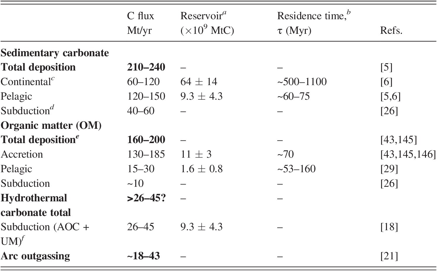
a Reservoir size from Ref. Reference Hirschmann83.
b Residence time is estimated by assuming a homogeneous reservoir and by dividing reservoir size by flux. Because geological reservoirs are heterogeneous, the mean age of C in those reservoirs should greatly exceed their theoretical residence times.
c Obtained from the difference between total deposition flux and total pelagic deposition flux provided by Ref. Reference Wallmann5.
d Note that the Cenozoic average estimated by Ref. Reference Clift26, in part based on Ref. Reference Plank and Langmuir25, exceeds the estimate from Ref. Reference Kelemen and Manning21. The pelagic deposition flux exceeds the carbonate subduction flux, which suggests net accumulation of carbonate in the pelagic reservoir.
e This total contains a fraction of partially graphitic petrogenic materials, estimated by Ref. Reference Galy, Peucker-Ehrenbrink and Eglinton33 to be around 40 Mt/yr. The large spread of estimates of organic carbon (OC) burial (as in Ref. Reference Cartapanis, Bianchi, Jaccard and Galbraith29) is in part due to the variety of depositional environments considered and to the different definitions of what “burial” of biospheric OM means for different authors. For example, the estimates of Ref. Reference Berner43 (on which the re-evaluations of Ref. Reference Smith, Bianchi, Allison, Savage and Galy145 are based) accounts for a global 20 wt.% diagenetic loss by decarboxylation before OC is effectively “buried.” Loss of hydrocarbons during catagenesis in accretionary wedges may reduce by another 20% or more (>25 Mt/yr) the amount of OC that eventually subducts.
f AOC = altered oceanic crust (22–28 Mt/yr); UM = hydrothermally altered upper mantle (4–15 Mt/yr), after Ref. Reference Kelemen and Manning21.
To understand the link between oceanic carbon deposition centers and modes of long-term carbon cycling, we need to consider the fate of sedimentary carbon. Shelf and oceanic island carbon mostly escapes subduction and is accreted to continents during continental subduction and collision. While a fraction of pelagic carbon can also be thrusted within accretionary wedges and accreted, mostReference Clift and Vannucchi10 is bound to be subducted, dissolved, or molten at various depths (Figure 10.1) within the sinking plate, before being released in the fore-arc,Reference Mottl, McCollom, Wheat and Fryer11 arc,Reference Allard12 or back-arc regions,Reference Sakai13 or mechanically incorporated deeper into the mantle. The contrasted fate distinguishes two principal modes of tectonic carbon cycling: the shallow accretionary carbon cycle and the relatively deeper subduction zone carbon cycle (Figure 10.1). What is not clear yet is how fast those cycles operate and how they interact.
The major carbon (organic and inorganic) transformation pathways in subduction zones (layout adapted from Ref. Reference Canfield, Glazer and Falkowski144). Processes that mediate these transformations are hydrothermal alteration – including reverse weathering – of the oceanic crust (seafloor), slab and mantle wedge (infiltration), sedimentation, diagenetic (CO2) and catagenetic (e.g. CH4) degassing of kerogen, graphitization by pressure, temperature, and deformation, dehydration of slabs, electron transfers (redox) between Fe-, C-, and S-bearing mineral and liquids, melting, and reactive transport (assimilation/deposition) of C-bearing fluids and melts from slabs to the exosphere through mantle wedge and continental crust. Dehydration of slabs and partial melting are indicated by blue and red droplets, respectively. A potential limit to deep C subduction in the transition zone is indicated.Reference Thomson, Walter, Kohn and Brooker84

The residence time of carbon in all geological reservoirs is important because it controls the response of the lithosphere‒climate system to perturbations in carbon fluxes,Reference Sleep and Zahnle14 and long-term changes in the partitioning of oceanic carbonate may cause such perturbation. The key is that the fluid reservoirs (atmosphere, ocean, biosphere) contain so little carbon that even slight perturbations of subduction or degassing fluxes may change the size of the surface carbon reservoir and impact climate and the diversity of surface habitats over timescales that are instants in the context of geological time. To the first order, the residence time of carbon in the subduction zone depends on the efficacy of shallow subduction processes (<~150 km) to return carbon back to the atmosphere and ocean, and this can occur within timescales of ~10 Myr (Figure 10.1). The residence time of carbon in continents depends on the interaction/assimilation of continental carbon materials by arc magmasReference Lee15, Reference Mason, Edmonds and Turchyn16 and on orogenic processes of continental C degassing.Reference Foley and Fischer17, Reference McKenzie18
This contribution reviews the processes that transform and transport carbon materials in the subduction environment. We first introduce how surface and deep processes control the fluxes of carbon in and out of the solid Earth through subduction zones. Those fluxes define what we call the pace of the carbon cycle. Fast reorganization of Earth’s separating and amalgamating tectonic blocks is responsible for episodic modifications of carbon fluxes. We call these fluctuations the pulse, or cadence, of the carbon cycle. The carbon isotope record and other proxiesReference Krissansen-Totton, Buick and Catling19 suggest that the geological carbon cycle has been uninterrupted for more than 3 Gyr. We call this last property its longevity. Many recent advances illuminate the origin and controls of each of these central carbon cycle properties. Our work shows that only a cross-scale understanding in space and time will illuminate the links between the microscopic processes of the carbon cycle and patterns of macroscopic evolution, providing a toolkit to decipher the meaning of atmospheric signatures on Earth and other planets (Figure 10.2).
The tectonic carbon cycle is a hierarchical structure that must be studied at all scales of organization. The materials that comprise the carbon cycle and their transformations affect the higher levels of organization that transport carbon through the surface and deep Earth. In turn, the tectonic evolution of our planet influences the transformation of carbon-based geobiomaterials and the nature of the reactions that mediate those transformations. As a structure coproduced by biological and geological evolution, the subduction carbon cycle is the ideal research target to assess the link between the heterogeneity of Earth’s materials, their reactivity, and the patterns of macroscopic evolution such as cyclicity, irreversibility, continuity, and disruption.

10.2 How Do Surface Processes Control the Subduction Carbon Cycle?
10.2.1 Sources to Sinks and Back
Subduction zones act both as a source and a sink of carbon for the exosphere. Over geological timescales, the source is the volcanic flux of carbon degassed in continental and oceanic arcs, while the sink is the carbon subducted in both reduced (organic C) and oxidized (carbonate) forms. But subduction fluxes do not depend on tectonic processes and mantle convection only; they are also controlled by surface processes driven by solar energy and tied to the water cycle.Reference Campbell and Taylor20 The overwhelming majority of carbon subducted is allochthonous,Reference Kelemen and Manning21 which means that most of it is added to marine sediments and the oceanic lithosphere from external sources – mainly the oceans and continents. The fate of carbon in subduction zones is therefore under tight oceanographic, biological, and geomorphic control (Figure 10.1), and it is especially sensitive to the partitioning of carbon between deep (pelagic) and shallow (e.g. shelves, oceanic plateaus) oceanic domains.Reference Caldeira22
There are three main carbon sinks, or pumps, that mediate the transfer of allochotonous carbon from oceans to sediment and the oceanic lithosphere: the hydrothermal carbon pump, which stores CO2 within the oceanic lithosphere during seafloor weathering; the soft-tissue pump, which leads to accumulation of soft organic tissues (of terrestrial or marine origins) in seafloor sediments; and the carbonate pump, which controls the topology of the carbonate compensation depth above which carbonate sedimentation on the seafloor may occur and below which carbonates are undersaturated and may lead to dissolution of old CaCO3 already deposited on the seafloor.Reference Archer23, Reference Zachos24
10.2.2 Heterogeneity of Sedimentary Carbonate Subduction (Carbonate Pump)
Knowledge of carbonate heterogeneities on the seafloor and of carbon subduction rates mostly comes from recent decades of deep-sea drilling efforts.Reference Plank and Langmuir25 Continuous core sampling of sedimentary covers and upper oceanic crust offers a direct window onto what rocks may eventually subduct and degas. Today, most marine carbonates form and accumulate in the Atlantic and Indian Oceans, where few subduction zones have formed yet, and to a lesser degree on top of the ridges of the southeast Pacific. Estimates of total annual carbonate subduction range between ~66 and 103 MtC/yr (Table 10.1), with about 60% present in sediments (~40‒60 MtC/yrReference Clift and Vannucchi10, Reference Plank and Langmuir25, Reference Clift26) and 40% in the altered oceanic lithosphere (~26‒43 MtC/yr in basalts and serpentinitesReference Kelemen and Manning21). Carbonate subduction fluxes have been less than total carbonate deposition rates over the Cenozoic (Table 10.1), which suggests net accumulation of pelagic carbonate.
While efforts are underway to reduce these large uncertainties, the most important limitation for past and future predictions of carbon cycle dynamics is the heterogeneity of the flux (Figure 10.3): 25% of the global carbon subduction flux of the last 10 MyrReference Clift26 has occurred in the Sunda trench. The importance of the Indonesian hot spot, as well as those of the Aegean and Makran (Figure 10.3), contrasts with the western Pacific, where subduction and degassing fluxes are generally low. But the southern Pacific New Hebrides–Solomon–Vanuatu segment does not conform to this rule. Unlike most settings of the western Ring of Fire, the slab is young and plunges to the east. The system is long and so is rich in carbonate,Reference Clift26 which it is a sizable contributor to the global subducted carbon inventory (Figure 10.2). Allard et al.Reference Allard12 showed that the Ambrym volcano in the Vanuatu islands pours out slab carbon at a record rate (~5–9% of the global volcanic carbon flux), providing a unique window onto the unusual CO2 productivity of this young arc system.Reference Johnston, Turchyn and Edmonds27
Contribution of selected subduction zones to global sedimentary C subduction flux. Fluxes are from Ref. Reference Clift26, where length of subduction zones and carbon (organic and inorganic) concentrations in trench sediments are compiled (see also Ref. Reference Plank and Langmuir25). Note that the computation of flux includes corrections for sediment porosity used but not reported in Ref. Reference Clift26. Rate of carbon subduction are provided in t/km/yr for each subduction zone. Organic carbon is in gray and black, and black circles denote OC hot spots. Inorganic carbon is in pale and dark blue, with dark blue denoting hot spots. The fractional contribution of each subduction to the global sedimentary C flux is indicated as a percentage of total inorganic (blue) or organic (black) carbon subduction, respectively, in the histogram of the right panel (cf. Table 10.1). Note that the flux associated with basalt, gabbro, and ultramafic carbonate is not included. This corresponds to an additional subduction rate of ~850 ± 200 tC/km/yr.

10.2.3 Hot Spot of Organic Carbon Subduction in the Sub-Arctic Pacific Rim (Soft Tissue Pump)
A heterogeneous distribution and diversity characterize the soft tissue pump,Reference Arndt28 as well as the subduction of organic carbon (OC). The burial of subductable OC in pelagic environments represents a flux of up to 10–30 MtC/yr over the last 150 kyr (Figure 10.2),Reference Cartapanis, Bianchi, Jaccard and Galbraith29 and perhaps during most of the Phanerozoic.Reference Hayes and Waldbauer2 Though modest compared to net primary productivity (~100 Gt/yr),Reference del Giorgio and Duarte30 this weak but continuous isolation of organic reductants in sediments and rocks is essential for the persistence of atmospheric O2 levels that are so high and so far from thermodynamic equilibriumReference Krissansen-Totton, Bergsman and Catling31 over geological timescales.
Just like carbonate, OC subduction is geographically heterogeneous,Reference Clift26 but its deposition hot spots are elsewhere (Figure 10.3). The trenches of Alaska, the Aleutians, and British Columbia contribute ~23% of global OC subduction, while many other trenches, such as those of the western Pacific and Central America, are comparatively marginal. This is either because the trenches are small or because sediments do not contain much OC (Figure 10.2). This heterogeneity seems primarily controlled by continental erosion, weathering, and marine sedimentation rates. The northern Pacific hot spot is dominated by subduction of thick sequences of terrigenous sediments.Reference Cui, Bianchi, Jaeger and Smith32 Surprisingly, all OC subduction hot spots are associated with the subduction of deep-sea turbiditic sequences, such as Surveyor fan (Alaska) and Indus fan (Makran) (cf. Figure 10.3). The OC fraction derived from terrestrial sources (petrogenic and biologicReference Galy, Peucker-Ehrenbrink and Eglinton33) can locally reach more than 70% in active margin sediments.Reference Blair and Aller34 This means that the geomorphic and climatic conditions that influence the export of organic-rich tropical, Arctic, and mountainous sedimentsReference Hilton35, Reference Hilton36 to the marine environmentReference Husson and Peters37 are the same as those that control the pattern of OC subduction, too. Hence further research is needed to elucidate the link between continental configuration in the Wilson cycle, erosion/sedimentation patterns, and OC burial, with special attention paid to active margins.Reference Bao38
Unlike carbonates, which conserve their structure across a broad range of pressure and temperature conditions of Earth’s interior, aging biomolecules display stunning plasticity in structure and compositionReference Beyssac, Rouzaud, Goffé, Brunet and Chopin39–Reference Adam, Schneckenburger, Schaeffer and Albrecht41 acquired during transport and transformation through the lithosphere (Figure 10.2). It is often assumed that graphite is the main form of OC in rocks. However, organic macromolecules (e.g. kerogens) may not become proper crystalline graphite before the late stages of the subduction process (i.e. >600°C; Figure 10.1). The transformation of organic materials to their stable forms (e.g. graphite) involves a succession of metastable macromolecular intermediates called kerogens.Reference Helgeson, Richard, McKenzie, Norton and Schmitt42 Increasing temperature and the presence of water accelerates this process and drives the sequential release of CO2 (i.e. reduction of the kerogen residue) and then hydrocarbons (i.e. oxidation of the kerogens) from the kerogen residue in shallow, unconsolidated sedimentsReference Berner43 and in accretionary wedges (Figure 10.1).Reference Petrenko44 This so-called carbonizationReference Helgeson, Richard, McKenzie, Norton and Schmitt42 may decrease the amount of OC effectively subducted by 20–40% or more depending on whether or not hydrocarbons are trapped within the descending slabs. This is still an open question.
 (10.1)
Subsequent collapse of the kerogen structure involves 3D ordering of the carbon-rich aromatic backbone and is favored by pressure and shear.Reference Oohashi, Hirose and Shimamoto45 This structural ordering is called graphitization (Figure 10.1). First-principles approaches are now shedding light on the microscopic pathways involved in this process.Reference Berthonneau46, Reference Weck47 Because the transformations modeled by (10.1) are so slow in nature, it is even conceivable that the coldest slabs (e.g. the Mariana and the Aegean OC subduction hot spots) could reach the diamond stability field before completion of the carbonization and graphitization process. The graphitization process itself is irreversible, and field observations indicate that slabs may not lose much OC beyond 350–400°C.Reference Connolly and Galvez48, Reference Zhang, Ague and Brovarone49
The low reactivity of compact graphitic materials and their intricate weaving within poorly soluble mineral matrices explain why a graphitic fraction dislodged from rocks during erosion and weathering (18–104 MtC/yrReference Galy, Peucker-Ehrenbrink and Eglinton33) is continuously exported to the ocean (Figure 10.1). How much of this fossil petrogenic material subducts is not yet known, but it may represent 50% of OC in the trenches of South America.Reference Blair and Aller34
10.2.4 An Ancient Hydrothermal Carbon Sink
A last major contributor to allochthonous carbon incorporation to the oceanic lithosphere is hydrothermal carbonatization (Figure 10.1 and Table 10.1).Reference Alt50 More details are provided in a companion chapter in this book (Chapter 15). In short, the circulation of cold and carbon-rich seawater through the oceanic crust and mantle dissolves cations from the oceanic lithosphere. Elevated concentrations of cations and rising temperature have been responsible for cycles of carbonate deposition in oceanic hydrothermal systemsReference Alt51 today and in the past. Occurrences of carbonatized basalts have been reported as early as in the early Archean CratonReference Nakamura and Kato52 of eastern Pilbara (Australia) and in Archean greenstone belts.Reference Shibuya, Komiya, Nakamura, Takai and Maruyama53 They suggest that: (1) carbonatization of the lithosphere may have been the means by which the atmosphere lost its primordial CO2Reference Ueda, Sawaki and Maruyama54; and (2) carbonatization of the lithosphere may have been the only flux of global importance capable of balancing outputs from the deep Earth during the Archean, Proterozoic, and large swaths of the early Phanerozoic (Figure 10.1). Therefore, surface biogeochemical processes involving the water cycle may have controlled the magnitude and longevity of carbon inputs to subduction zones since their initiation, more than 3 Ga.Reference Dhuime, Hawkesworth, Cawood and Storey55 The above shows that the pelagic reservoir is not at steady state over the Cenozoic. What about the subduction zone itself?
10.3 Is the Subduction Zone Carbon Neutral?
To the first order, the parameter that is most likely to affect models of atmosphere–climate–lithosphere evolution over geological time (<100 Myr) is the subduction efficiency, σ (Figure 10.1). This macroscopic parameter is the fraction of subducted carbon that penetrates beyond sub-arc depths in subduction zones (cf. Figure 10.1).Reference Kelemen and Manning21, Reference Sieber, Hermann and Yaxley56 For a given subduction flux, the lower the parameter σ, the faster the response of the geological carbon cycle to perturbations in flux at the inlet of the subduction system.
Johnston et al.Reference Johnston, Turchyn and Edmonds27 compared inventories of global input to and output from selected subduction zones to determine their efficiency. After correcting for possible mantle and continental contributions,Reference Mason, Edmonds and Turchyn16, Reference Aiuppa, Fischer, Plank, Robidoux and Di Napoli57 Johnston et al. found that 18–70%Reference Kelemen and Manning21, Reference Clift26 of the input (Table 10.1) might be accounted for by arc carbon emissions derived from the slab, setting σ to ~0.3–0.8. Corrections are needed because the accretionary and subduction cycles intersect when arc magma rises through the continental crust and that magma assimilates a fraction of the carbon that had been accreted to continents during previous collisional events (Figure 10.1).Reference McKenzie18 This phenomenon is thought to control the important emissions in Italy (e.g. Etna, Vesuvius), parts of the Andes, and IndonesiaReference Chiodini58 today. The estimates of Johnston et al. can be compared with estimates from Table 10.1, we find σ of ~0.4–0.9. This is consistent, and it shows that a sizable fraction of subducted carbon does not take the short path out to the exosphere and continuously accumulates anywhere between the mantle wedge and the transition zone. The mismatch between input and volcanic output of slab carbon suggests that subduction zones, in their present configuration, act as a net sink of carbon over timescales of about 10‒50 Myr.
But the meaning of a mismatch itself is unclear. Fundamentally, volcanic arcs are indicators of slab dehydration and partial melting in the mantle,Reference Campbell and Taylor20, Reference Stolper and Newman59 and the two processes are only indirectly linked to C loss from slabs. For example, dehydration at sub-arc depths for cool and cold slabs (e.g. Tonga, Mariana) drives increased fluid flux into the mantle wedge, producing higher degrees of partial melting and a greater proportion of carbon transport to the volcanic front (western Pacific).Reference Allard12 By contrast, hot and warm slabs promote carbon dissolution at shallower depths and may release carbon away from the volcanic fronts (e.g. Cascadia and Central America). Therefore, cooling of Earth is thought to have changed the pace of subduction carbon cyclingReference Sleep and Zahnle14 slowly, over a billion-year timescale: a hotter Precambrian Earth would have returned more carbon faster from the carbonatized lithosphere, while cooler slabs that are denser and rich in garnetReference Bjørnerud and Austrheim60 would promote penetration of carbonates to sub-arc depth and beyond.
This trend is only qualitative, and complementary approaches are required to quantify the fluxes and to assess their controlling factors. We take a broad-level look at three underlying mechanisms that control the partitioning of carbon between rocks and fluids in the most inaccessible parts of the subduction zones ‒ the slab, mantle wedge, and arcs themselves: (1) the problem of carbon solubility in fluids and its underlying mineralogical controls; (2) the problem of fluid production within slabs; and (3) the problem of fluid reactivity along their paths from the subducted lithosphere to the surface.
10.4 How Rocks Influence the Solubility of Carbon
The composition of subducting slabs differs from that entering the subduction system. Open system processes – in which rocks are infiltrated by fluids and melts (also referred to indiscriminately as liquids) – control how much and how fast carbon is removed from slabs. The greater the amount of carbon released by dissolution and melting at fore- and sub-arc depths (Figure 10.1), the faster the subduction cycle may respond to any kind of perturbation in flux. Carbonates are the most abundant form of carbon in slabs (Table 10.1), and most box models of the geological carbon cycleReference Berner, Lasaga and Garrels61 represent the fate of carbonate by progress of the so-called reverse Urey reactionReference Goldschmidt62:
However, this reaction is also a model, an aggregation of many processes.Reference Berner63 It is therefore not a mechanistic explanation of the dissolution process. The last decade has offered valuable insights into the microscopic complexity of Urey-type “decarbonation” reactionsReference Galvez and Gaillardet4 and their macroscopic expressions as carbon fluxes.
10.4.1 Dissolution by Rising Pressure and Temperature: Which Silicate Is in Charge?
An essential but implicit meaning of (10.2) is that the release of C from slabs is linked to that of water – the solvent and catalyst for the reaction. Carbon release tracks the main sequence of fore-arc and sub-arc mineral dehydration reactions.Reference McGary, Evans, Wannamaker, Elsenbeck and Rondenay64 The most important of these reactions are the destabilization of lawsonite/epidote during eclogitization of the altered oceanic crustReference Poli, Franzolin, Fumagalli and Crottini65 at ~450–700°C and the dehydration of antigorite/chloriteReference Ulmer and Trommsdorff66 in the serpentinized oceanic mantle. Both take place at around the same temperature, but the second pathway occurs deeper in the subduction zone because deserpentinization and dechloritization reactions occur in the altered ultramafic rocks of the lower and usually colder section of the descending slab (Figures 10.1 and 10.4).
Devolatilization pattern (H2O and C) in a subducting slab and its link to subduction efficiency. The latter is the fraction of subducted carbon released at fore-arc and sub-arcs depths (cf. Ref. Reference Volk3). The results are only qualitative and are based on ongoing studies investigating the coupling between C, H, Na, K, Si, and Al cycles in open subduction-zone systems.Reference Galvez, Connolly and Manning67 The shallow output flux depends on the hydration structure of the oceanic lithosphere, and conceivably, on the degree of partial melting (red tones). Overall, this flux varies between ~15 and 50 MtC/yr (i.e. in the order of magnitude of arc emissionsReference Kelemen and Manning21, Reference Johnston, Turchyn and Edmonds27), between 0.1 and 0.6 of the incoming flux, and more likely ~0.4–0.5 in the Cenozoic (correspond to σ of ~0.5–0.6; cf. Figures 10.6 and 10.7). This ratio may have approached 0 in the Paleozoic and Mesozoic (i.e. before the rise of pelagic calcifiers). This should be considered in long-term models of Phanerozoic carbon cycle evolution.

Another insight from (10.2) is that the solubility of carbonates in hydrous fluids is primarily controlled by the relative stability of the various silicates (e.g. wollastonite, garnetReference Galvez40) in which they transform; in other words, the rapid rise of C solubility at the onset of garnet formation in most sediment and mafic lithologiesReference Galvez, Connolly and Manning67 reflects the increasing relative stability of calc-silicates with rising temperature:
 (10.3)
This process is an incongruent dissolution,Reference Galvez, Connolly and Manning67 where M is a divalent metal Ca, Mg, Fe, or Mn.
In practice, the congruent or incongruent nature of the dissolution depends on the kinetics of dissolution, the thermodynamic properties of calc–silicates, the kinetics of calc–silicate precipitation, and the rate of fluid transport.Reference Galvez40, Reference Galvez, Connolly and Manning67 Recent thermodynamic analysis, however, suggest that congruent pathways may be restricted only to very high pressures and low temperaturesReference Galvez, Connolly and Manning67; regimes where fluid fluxes tend to be low. In addition, the ubiquitous presence of calc–silicates such as lawsonite down to 350°C in most silicic and aluminous lithologiesReference Tsujimori and Ernst68 supports the idea that their formation is not kinetically limited in the subduction zone. Hence, field and thermodynamic evidence suggests that incongruent pathways have been the most important in driving the dissolution of carbon along most subduction geotherms, today and in the geological past).
This general rule may not hold in the case of dolostone and limestone lithologies. These rocks usually lack the alumina and, in the most extreme case, silica that promote vigorous dissolution (10.2 and 10.3). In addition, marble lithologies are also rather dry and also notably impermeable to fluid flow, and therefore not prone to dissolution. Yet dissolution reactions may also be sustained by chemical disequilibrium between contrasted lithologies even when pressure and temperature are invariant. For example, diffusion of volatiles (H2OReference Ague69 or H2Reference Galvez40) and nonvolatile elements (Al and SiReference Ague and Nicolescu70) into the marbles may modify a(CO2), or the stability of calc–silicates (10.2 and 10.3) and drive reactions (10.2) and (10.3). In fact, field evidence shows that when dissolution of marbles does occur, it tends to be restricted to the vicinity of fracturesReference Ague and Nicolescu70 and tectonic discontinuities,Reference Ague69,7Reference Sleep1 precisely where fluids rich in Al and Si can circulate and boost carbon dissolution processes. Therefore, it is likely that incongruent pathways play the dominant role in carbon mobilization from slabs at subsolidus conditions. The growing importance of deep-sea carbonates (carbonate oozeReference Pimm72) subduction in the next 100 million years (Table 10.1) makes them obvious targets for future research focusing on their peculiar mechanical properties and open-system behavior at elevated pressures and temperatures.
10.4.2 Carbonate Melts from Hot Slabs and Diapirs?
Partial melting of the slab may start at >900°C in the presence of water. It can affect the top section of hot slabs (e.g. Aleutians/Mexico) when it is infiltrated by water, and it may also occur in unusually hot and buoyant fragments of slab sediments in the mantle wedge.Reference Gerya and Yuen73 The process forms ionic melts that are rich in carbonate components (i.e. hydrous carbonatites),Reference Skora74 but the thermodynamic,Reference Kang, Schmidt, Poli, Franzolin and Connolly75 structural,Reference Foustoukos and Mysen76 and rheological properties of those compositionally heterogeneous melts remain largely unknown. Assessing their properties is important because carbonate melts are highly mobile, highly reactive,Reference Russell, Porritt, Lavallée and Dingwell77 and important carriers of carbon beyond sub-arc depth anywhere between ~100 km and 400–600 km within the slab and in the mantle wedge. A few implications follow:
(1) In carbonate bearing lithologies, formation of metamorphic garnet (e.g. grossular), the ubiquitous silicate mineral of high-pressure metamorphism, may be the most practical and important indicator of both dehydrationReference Baxter and Caddick78 and C redistribution (e.g. carbonate dissolution) between rocks and fluids via Urey-type processes (Figure 10.4).
(2) Carbon cycling in the slab is a problem of transportReference Frezzotti, Selverstone, Sharp and Compagnoni79 where dehydration, decarbonation, desilicification, and dealuminification of rocks are parts of a single overarching problem.Reference Galvez, Connolly and Manning67 Work is underway to link the microscopic properties of geo-fluids (aqueous, carbonate, silicate) and minerals with macroscopic patterns of element transport across shallow lithospheric reservoirs.Reference Connolly and Galvez48, Reference Galvez, Connolly and Manning67, Reference Galvez, Manning, Connolly and Rumble80
(3) There is a growing consensus, informed by thermodynamic models, that pulses of carbon release from slabs by subsolidus dissolution do occur around 500–800°C, representing an overall flux of between ~10 and 40 MtC/yr between ~80 and 140 km depth below the volcanic arc.Reference Connolly and Galvez48, Reference Gorman, Kerrick and Connolly81, Reference Connolly82 This flux is uncertain, but overall it is consistent with volcanic emissions.Reference Kelemen and Manning21 The pulsatile character (Figure 10.4) of the flux, however, is primarily due to the timing and volume of H2O infiltration rather than to the thermodynamics, or kinetics, of the Urey-type reactions. This is important because it means that the subduction efficiency σ, as opposed to total carbon release, is controlled by where H2O is concentrated within the hydrated slab, rather than by the absolute amount of H2O contained in it. Only the water contained in the uppermost 10 km of slab mediates the fast cycling of carbon in the fore-arc and sub-arc regions.
(4) The parameter σ may not be a mere parameter at all over geological timescales. It is more likely to be a variable that is dependent on the nature of carbon inputs. Indeed, we have shown that limestones and carbonatized lithosphere rocks behave differently, both mechanically and chemically. For example, while σ of ~0.4–0.8 in the Cenozoic (Table 10.1) is characterized by important subduction of limestones (Table 10.1), this value may have vanished during most of the Precambrian, Paleozoic, and early Mesozoic, stranding carbon in shallow surface reservoirs. Interestingly, this idea is qualitatively consistent with recent isotopic and geochemical proxies,Reference Hirschmann83 which suggest a net growth of the continental and pelagic carbonate reservoir (Table 10.1) over the last 2 Gyr.Reference Hayes and Waldbauer2, Reference Hirschmann83
10.4.3 Where Is the Barrier to Deep Carbon Subduction?
Global budgets are sensitive to thermal models and the permeability/rheology of rocks within the slab. Therefore, slabs that are cold and/or covered by thick and impermeable carbonate layers should retain a significant fraction of their carbon cargo to beyond sub-arc depths. What is the fate of carbon beyond this limit (Figure 10.1)?
If carbon makes it beyond sub-arc depths (~150 km), it may not push much further beyond the transition zone (~410–660 km). The reason for this is the existence of a deep depression in the temperature (1000–1100°C) at which anhydrous carbonated oceanic crust melts at uppermost transition-zone conditions.Reference Thomson, Walter, Kohn and Brooker84 Thomson et al. showed that the curvature of the solidus of carbonated eclogite is also controlled by the partitioning of nonvolatile elements, chief among them calcium and sodium, between mineral phasesReference Thomson, Walter, Kohn and Brooker84 in high-pressure eclogites. Most geotherms should intersect this melting barrier.
To the best of our knowledge, there is as yet no experiment that quantifies the effect of water on the topology of the anhydrous solidus of carbonated eclogites in the vicinity of the deep curvature (i.e. at the conditions of the transition zone around ~10–20 GPa). Qualitatively at least, it is now undisputed that increasing activity of water a(H2O) dampens the solidus of carbonate rocks,Reference Skora74, Reference Wyllie and Tuttle85 bringing their temperature of melting closer to 900–1000°C, promoting the formation of carbonate melts. This principle applies to carbonatized basaltic lithologiesReference Poli86 in particular and to all carbonate-bearing systems in general, typically those rich in iron and manganeseReference Kang and Schmidt87 that are relevant for the fate of subducted banded iron formation in the Archean Earth. This should limit even more the possibility of carbon subduction through the transition zone (Figure 10.1).
10.4.4 Are Thermal Anomalies the Norm?
There is a growing consensus that the relevant pressure–temperature trajectories of slab materials may be hotter than most canonical models assume.Reference Gorman, Kerrick and Connolly81 First of all, there is an apparent incompatibility between slab thermal models predicted by theoryReference Syracuse, van Keken and Abers88 – usually cold – versus those inferred from phase assemblage relations and mineral chemistryReference Penniston-Dorland, Kohn and Manning89 – generally warmer. Second, the mantle wedge may be populated by detached fragments of slab sediments (e.g. diapirsReference Gerya and Yuen73) that are thought to follow hotter pressure–temperature trajectories than the rest of the slab (Figure 10.1). It is important because it implies that the production of hydrous carbonatite melts may be more common than expected, particularly for cold slabs (e.g. Aegean) covered by kilometer-thick buoyant sedimentary piles. Overall, research into the thermal regime of slab materials may eventually redefine what thermal normality is in the subduction environment.
Taken together, the possibility of paths that are hotter than normal for most subducted sediments and the existence of a chemical barrier to deep carbonate subduction (Figure 10.1) means that most subducted carbon must have been stranded above the transition zone through most of Earth’s history.Reference Kelemen and Manning21 However, there remain important uncertainties on the subduction efficiency, in particular, its variability in space and time. This uncertainty hinders quantitative understanding of the response dynamics of the carbon cycle to perturbations.
10.5 Transport and Reactivity of Carbon-Bearing Liquids
Aqueous fluids and carbonatitic melts produced in the slab are predicted to be mobile due to their low viscosity. But crustal liquids are not passive carriers of carbon back to the surface. They re-equilibrate continuously with changing environmental conditions across the crust and mantle. Both carbonate and elemental C (graphite/diamond) may form along the way and delay the return of subducted C to the exogenic cycles. It may take anywhere from thousands to millions of years for the mobilized carbon to return to the exosphere.
Transport of fluids and melts occurs mostly along lithological interfaces and other discontinuities, such as faults and fractures (see Figure 10.4 and Supplementary Materials at the end of chapter) in the heterogeneous interface between slab and mantle,Reference Angiboust, Pettke, De Hoog, Caron and Oncken90 and within the rocky mantle itself.Reference McGary, Evans, Wannamaker, Elsenbeck and Rondenay64 This is observed in the fieldReference Galvez71 and via geophysical observations of fluid migration through the mantle wedge.Reference Worzewski, Jegen, Kopp, Brasse and Castillo91 The fate of C-bearing liquids during their ascent through the slab, mantle wedge, and overriding crust is controlled by four critical variables: pressure/temperature, redox state, activity of silica, and activity of water.
10.5.1 Pressure and Temperature
For the same reason that rising pressure and temperature enhances the solubility of carbonates in subducting slabs, downward temperature paths, too, may lead to carbonate precipitation out of fluids ascending along and across the slab. This chromatographic process is predicted thermodynamicallyReference Ague69 and is observed in the field.Reference Piccoli, Brovarone, Beyssac, Martinez, Ague and Chaduteau92 This illustrates that there is a delay between the time carbon is dissolved from the slab and the time it eventually reaches the surface.
10.5.2 Low- and High-Temperature Redox Processes
The redox state, too, is important for the fate of both carbonates and organic materials, and it is usually measured by the thermodynamic activity of oxygen. Carbon can bond to both oxygen and hydrogen, and the balance between oxygenated species (e.g. CO2) and hydrogenated carbon species (e.g. CH4) in a fluid–rock system depends on the nature and abundance of other “redox” elements in the rock, such as Fe (Fe2+, Fe3+), Mn, and multiple S species susceptible to exchanging electrons with carbon.Reference Tumiati, Godard, Martin, Malaspina and Poli93 But there is a limit to the amount of C a fluid can contain at typical subduction-zone conditions. This limit is fixed by thermodynamics, and varies with pressure, temperature, and rock composition.Reference Galvez, Connolly and Manning67, Reference Connolly and Cesare94 If graphitic materials are stable – as is usually the case in subducted sediment (Figure 10.4) – then the so-called graphite-saturated COH system imposes a minimum in carbon solubility midway between fluids dominated by CO2 and fluids dominated by CH4.Reference Connolly and Cesare94 The existence of such a minimum is important because it implies that quasi-static changes in pressure, temperature, a(H2O), or fO2 of a graphite- or diamond-saturated fluid could involve both carbon dissolution and/or precipitation of the fluid. Therefore, C may be locked in the form of graphite during fluid ascent through the slabReference Galvez40, Reference Brovarone95 or through the continental crust,Reference Weis, Friedman and Gleason96, Reference Rumble, Duke and Hoering97 creating complex locking and unlocking pathways for deep carbon (Figure 10.5).
Redox pathways in the subduction zone. Graphite precipitation from carbonate at a lithological interface. (a) Field image of the outcrop in Alpine Corsica.Reference Galvez40 (b) Representative COH diagram showing the curvature of the C-saturation surface at the elevated pressures and temperatures typical of subduction zones, illustrating various pathways leading to elemental carbon precipitation.

Fluctuations in redox conditions may occur anywhere from the shallow to the deep subduction zone. For example, it has been shown that serpentinite assemblages maintain their reducing power in the shallow subduction zone at conditions lower than 10 kbar and 500°C.Reference Malvoisin, Chopin, Brunet and Galvez98 Those conditions may cause the spontaneous formation of refractory graphite from carbonate according to:
 (10.4)
There is now evidence for such a mechanism occurring at temperatures of no more than 450°C (Figure 10.4).Reference Galvez40, Reference Galvez71 A redox mechanism formally analogous to (10.4) is thought to occur below 250 km, too, where carbonatite melts expelled from the slab re-equilibrate with mantle lithologies where metallic iron is stable (Figure 10.1).Reference Rohrbach and Schmidt99 Mutual re-equilibration between carbonatite melts and mantle rocks involves the spontaneous production of diamond according to:
 (10.5)
10.5.3 SiO2 Activity
Just like a(SiO2) influences the dissolution of C in hydrous fluids of slabs via Urey-type reactions (cf. (10.2) and (10.3)), fluctuations of a(SiO2) impact the behavior of C in all types of subduction-zone liquid in which it may dissolve. This is particularly true of carbonate and other alkaline melts. Experimental worksReference Russell, Porritt, Lavallée and Dingwell77, Reference Dalton and Wood100 have shown that dolomitic melts formed in the descending slab degas at the contact of peridotitic mineral assemblages characterized by comparatively higher a(SiO2) (orthopyroxene and clinopyroxene).
 (10.6)
This mechanism may supply large fluxes of diffuse CO2 outgassing with decompression, as the melt dissolves more silica or any other acidic component. Therefore, cataclysmic eruptions (kimberlitesReference Jones, Genge and Carmody101) may ensue if those melts stall for long periods of timeReference Sleep1 in environments such as the base of the continental crust.
10.5.4 Water
Just like surface processes, many processes of the slab–mantle wedge interface involve repeated cycles of fluid desiccation, whereby fast and near-quantitative redistribution of H2O from fluids toward solid (e.g. mantle wedge serpentinization) or melt phases occurs. Desiccation is a possibly dominant mode of elemental carbon sequestration in the crust and upper mantle, although this mechanism has received little attention so far. Because the solubility of water in silicate melts that are poor in alkalis is greater than that of carbonic species,Reference Stolper, Fine, Johnson and Newman102, Reference Mysen103 rehydration (below 600°CReference Pirard and Hermann104) and flux melting of the mantle wedge by infiltrating COH fluids may form restitic graphite/diamond (Figure 10.5b) via:
This mechanism is supported by theory (Figure 10.5); evidence for it in nature may be found in the Kokshetav massif (north Kazakhstan)Reference Korsakov and Hermann105 or in Lianoning (northeast China),Reference Zhang, Yu and Jiang106 where the association of graphite with jadeites is intriguing.
Overall, a combination of physicochemical processes drive not only carbon loss from slabs, but also its reactivity and fate in the heterogeneous chromatographic columns that separate slab liquids from the surface. Therefore, a carbon flux at the surface of Earth (or of any planet) does not mean an active release is operating.
10.6 Carbon Dynamics at the Subduction/Collision Transition
Surface, subduction, and mantle processes control the fluxes of C. But numerous past instances of climatic and carbon cycle perturbationsReference Rothman, Hayes and Summons107 show that changes in geological fluxes occur continuously on Earth. Subduction zones evolve, may change polarity,Reference Cooper and Taylor108 and even vanish in complex collision zones. The subduction/collision transitionReference Hoareau109 illustrates how quickly the reorganization of Earth’s tectonic building blocks may cause imbalances in the geological C cycle (Figure 10.5). We refer to these episodic changes as the pulse of the carbon cycle.
The collision zoneReference Pubellier and Meresse110 is a dominant pathway of carbon processing,Reference Condie and O’Neill111 particularly in the Indo-Pacific region today (Ontong Java in the Vanuatu–Solomon arc) and in the former Tethyan orogens.Reference Selverstone and Gutzler112, Reference Tapponnier113 Docking of Greater India to Eurasia caused a situation of geodynamic instability marked by the Himalayan orogeny (Figure 10.6) that lasted for at least 50 MyReference Tapponnier113 and is still going on today at a reduced pace. Are the Himalayas carbon neutral over a geological timescale?Reference Gaillardet and Galy114 This is a question of timescales.
Examples of tectonic complexity at subduction zones: the collision factory. Long-range kinematic and dynamic reorganization in the western Pacific and Sundaland triggered by greater India subduction and collision; modified from Ref. Reference Jolivet147. The carbon budget of the collision zoneReference Gaillardet and Galy114 may only be resolved at the mesoscale (i.e. one that includes the orogen itself and the evolving subduction zones in its broad periphery).

On geological timescales, early workers proposed that the Tethyan orogeny as a whole would operate as a CO2 sink. The sink is due to enhanced silicate weatheringReference Raymo, Ruddiman and Froelich115 of freshly exhumed rocks and is usually modeled by the forward Urey-EbelmenReference Galvez and Gaillardet4 reaction (cf. (10.2)):
Recent studies provide insights into the complexity of this problem. Enhanced erosion, biotic OC burial,Reference Hilton, Galy and Hovius116 and accretion of pelagic carbonates to the growing orogenReference Selverstone and Gutzler112 operate as long-term CO2 sinks, while the weathering of petrogenic OCReference Hilton, Gaillardet, Calmels and Birck117 and enhanced sulfide weatheringReference Torres, West and Li118 counteract CO2 sources, at least transiently,Reference Torres, West and Li118 in much the same way as the interaction of orogenic magma with accreted carbonatesReference Mason, Edmonds and Turchyn16 or OCReference Tomkins, Rebryna, Weinberg and Schaefer119 in continents do (Figures 10.1 and 10.6). It is not at all clear how the acceleration of phosphorus and other nutrients exported to the marine basins surrounding the Himalayan orogen boosted net primary productivity, at least locally (i.e. another CO2 sink). The inventory and relevant timescales of these processes – surface or deep – are crucial to establishing a thorough carbon budget for an orogeny over geological timescales.
As part of this inventory effort, we propose that focusing on the orogen itself may still miss an entire – deeper – dimension of the tectonic disequilibrium caused by collision. Figure 10.6 shows how the collision of India with Eurasia since the Eocene involved large-scale coupling between continent–continent collision and slab subduction in the western Pacific and Southeast Asia (Sunda trench). The southeast-ward motion of lithospheric fragments of Eurasia was accommodated by lithospheric and asthenospheric reorganization east of the collision zone.Reference Sternai120 As a consequence, continental subduction and collision to the north have been accompanied by extension tectonics distributed over a 3000‑km region across the Sunda plate and western Pacific starting 45 Myr ago.Reference Royden, Burchfiel and van der Hilst121 We propose that slab retreat and rollback over this extended area may have boosted the pre-collisional CO2 source associated with the Sunda and western Pacific subductions, partly compensating for the sinks linked to the growing orogen itself. The mechanisms involved in a subduction acceleration are illustrated in the model of Section 10.7.
The result of tectonic and biological coevolution over the Cenozoic is one of long-term cooling, with a thermal maximum at the onset of the collision. Today, atmospheric CO2 is at a record low level, and the pace of the pre-anthropic subduction carbon cycle has reached a kinetic minimum.Reference Edmond and Huh122 Antarctica and Greenland ice sheets grew over the last ~30‒40 My. Degassing of the pelagic carbonates that have subducted beyond sub-arc depths over the Cenozoic and enhancements in pelagic sediment subduction in the future may boost the pace of the non-anthropogenic carbon cycle sometime in the next 100 Myr.
10.7 A Flavor of Life: A 3 Billion-Year-Old Record
The biosphere and geosphere are not separate entities. They are bound by the electron (redox) and proton (acid–base) transfer reactions of biological metabolism. Therefore, while Earth is the scaffold of biological evolution, the evolving style and longevity of the subduction-zone carbon cycle are in various ways indirect products of biological evolution (Figure 10.7). Four main milestones of this coevolution were: (1) the origin of cell death; (2) the evolution of the photosynthetic water-splitting complex; (3) the rise of multicellular algae and land plants; and (4) the advent of carbonate biomineralization. Life altered the geological cycle of electrons about 2.5 billion years ago and then the geological cycle of alkalinity, in the beginning indirectly, and then more directly.
Milestones in the coevolution of life, the surface environment, and the tectonic carbon cycle (see also Figure 10.2). The eons of biological innovations and adaptations are from Ref. Reference Falkowski and Godfrey131. Green tones denote biological transitions, blue tones denote geological transitions. (Upper Graph) The rise of atmospheric ozone and oxygen (Δ33S proxyReference Farquhar, Bao and Thiemens148), the meso/neoproterozoic rise of oxygen (δ56Cr proxyReference Cole149, Reference Canfield150), the evolution of bryophytes and vascular plants, and the evolution of pelagic calcifiers are highlighted (adapted from Ref. Reference Reinhard, Olson, Schwieterman and Lyons151). (Middle Graph) Statistical reconstruction of the carbonate isotope (δ13Ccarbonate) record through time.Reference Krissansen-Totton, Buick and Catling19 (Lower Graph) The statistical reconstruction of the global OC burial flux reconstructed from the North American sedimentary record from Ref. Reference Husson and Peters37 is also appended. Note that the sharp increase in OC burial flux at the “great unconformity”Reference Peters and Gaines138 that marks an order of magnitude rise in continental weathering and sedimentation through the early Paleozoic. GOE = Great Oxygenation Event; NOE = Neoproterozoic Oxygenation Event.

10.7.1 Biological Evolution Influences Carbon Subduction: First Milestone
Genomic studiesReference Soo, Hemp, Parks, Fischer and Hugenholtz123 and isotopic proxiesReference Krissansen-Totton, Buick and Catling19 place the origin of autotrophic life and respiration – the main carbon source and sink today – at some time in the Archean, but life alone did not affect the geological cycle of carbon as much as mortality did. Viral lysis of prokaryotesReference Bidle and Falkowski124, Reference Fuhrman125 and, possibly, genetically encoded death pathwaysReference Bidle and Falkowski124 may have played a disproportionate role in driving prokaryote mortality and, therefore, a primordial soft-tissue pump that helped the early biological necromass to spread across all marine habitats, including trenches and subduction zones. The ancestral origin of virusesReference Forterre and Prangishvili126 is at least qualitatively consistent with the idea that a sustained flux of dead organic materials from the sunlit upper ocean to the marine sediments may have been established at some time in the Archean. While it is conceivable that carbonatization of the oceanic crust, and its subduction, had been in place ever since oceans and the oceanic crust coexisted, it is the marine accumulation, isolation, accretion, and subductionReference Duncan and Dasgupta127, Reference Godderis and Veizer128 of organic reductants that sparked an OC cycle that was truly geological in scale.
10.7.2 Biological Evolution Influences the Dioxygen Cycle: Second Milestone
About 2.4 Gyr ago, the accumulation of OC in sediments, continents, and the mantle through subduction zonesReference Godderis and Veizer128 became, for the first time, tied to the production and eventual accumulation (about 2.33 Ga)Reference Hayes and Waldbauer2 of dioxygen gas in the lithosphere (in the form of iron oxides) and then in the exosphere.Reference Knoll129 The evolution of the water-splitting systemReference Fischer, Hemp and Johnson130 exploited, for the first time, the abundance of the water molecule as an almost unlimited source of protons and electrons for photosynthesis, releasing O2 as a highly reactive waste product.Reference Falkowski and Godfrey131
This redox pathway enhanced the stability of atmospheric CO2 (causing major glaciation, Figure 10.7), acidified riverine waters,Reference Halevy and Bachan132 and therefore may have boosted the weathering flux of essential nutrients (e.g. trace elements, phosphorus, etc.Reference Anbar133) from proto-continents to oceans. Life, therefore, exerted its first indirect control of the cycle of alkalinity and caused large-scale perturbations in the carbon cycle (Figure 10.7). A more subtle effect of this gradual redox shift was that it contributed to locking water on Earth, instead of water slowly escaping into spaceReference Catling, Zahnle and McKay134 as it did on Venus.Reference Driscoll and Bercovici135 This is important because water drives and lubricates the subduction-zone system and, through it, the entire carbon cycle. Therefore, the rise of redox disequilibrium between the fluid and solid compartments of Earth may have laid the ground for the exceptional longevity and vigor of Earth’s subduction carbon cycle.
10.7.3 Biological Evolution Influences the Cycle of Alkalinity: Third Milestone
About 1.5 billion years later, the biosphere enhanced its control on the geological cycle of alkalinity. The invasion of continents by algae and plants with roots in the early Paleozoic enhanced erosion and continental weathering.Reference Schwartzman and Volk136, Reference Hemingway137 Enhanced sediment export to the ocean boosted marine sedimentation of OC (Figure 10.7),Reference Husson and Peters37, Reference Peters and Gaines138, Reference Berner139 yet another potential process feeding back into the subduction carbon cycle.
10.7.4 Alkalinity Feeding Back into Biological Evolution: Fourth Milestone
The rising flux of dissolved weathering products (e.g. Ca) may have promoted further biological innovations. The geological record suggests algae evolved new ways to exploit the carbonate oversaturation state of the oceans over the Mesozoic.Reference Monteiro140 By accelerating chemical reactions, these organisms were able to reroute excess oceanic alkalinity to the carbonate skeleton and ultimately to rocks. The expansion of calcifiers to the distal parts of the oceans over the last 150 Myr boosted deep seafloor carbonate deposition and subduction. Therefore, the idea that a clear-cut dichotomy separates Earth’s biological processes (dominated by redox processes) and abiotic geochemical reactions (dominated by proton transfer chemistry)Reference Falkowski, Fenchel and Delong141 does not hold in the context of geological time (Figure 10.2). Fascinatingly, much of the biotic carbonate of the Atlantic and Indian oceans has yet to be subducted; when will the Atlantic Ring of Fire form? We do not know.
10.7.5 Response of Climate to the Enhanced Subduction of Pelagic Carbonates
The geological response to pelagic calcifiers is still very much ahead of us. The models of Figures 10.6 and 10.7 illustrate potential scenarios and the timescales involved. They illustrate how subduction zones are components of a larger dynamic system that includes continents, oceans, and biosphere. Figure 10.8 is simplistic, and it builds on much previous workReference Volk3, Reference Caldeira8; details are provided in the Supplementary Online Materials.
Non-steady-state response of the carbonate cycle to geodynamic and biological forcing: model design. The pelagic (Mp) and continental (Mc) carbonate reservoirs evolve by exchange of C (i.e. fluxes Fi) with the atmosphere and mantle (Figure 10.6). Mantle is assumed to be a reservoir of infinite residence time. The silicate weathering flux Fsw is linked to atmospheric temperature by a simple polynomial relation from Ref. Reference Berner, Lasaga and Garrels61. The C fluxes Fi are linked to Mi via rate constants ki (e.g. Fcm = kcmMc, and Fsub = ksubMp). The initial steady state is obtained with starting conditions chosen and updated from Ref. Reference Volk3 to be consistent with present-day values for C fluxes and reservoir sizes: Fi = 3 Tmol/yr, Fsw,i = 10 Tmol/yr (Ref. Reference Caves, Jost, Lau and Maher152); Fcw,i = 15 Tmol/yr (Ref. Reference Caves, Jost, Lau and Maher152); kcm = 0.00035, ksub = 0.0072, Mc,i = 7.583 × 10²¹ mol,Reference Hirschmann83 Mp,i = 0.917 × 10²¹ mol,Reference Hirschmann83 σ = 0.6 (see above), β = 0.25,Reference Volk3 ζ = 0. The system is solved analytically to find its steady state, which is close to present-day condition (i.e. Mc = 7.909 × 10²¹ mol (residence time τc ≈ 2800 Myr); Mp = 0.810 × 10²¹ mol (residence time τp ≈ 140 Myr); cf. Supplementary Online Materials). This steady state is then used for perturbation analysis (Figure 10.7).

We focus on the geological response of the carbonate cycle and atmospheric temperature to modifications in key geodynamic or biological parameters: β, the partitioning of carbonate between the pelagic and continental (accretion) environment; σ, the fraction of subducted carbon transported beyond sub-arc depths (Figure 10.3); and ζ, a self-amplification factor corresponding to the fraction of continental carbonate degassing that is controlled by arc magmatism. The pelagic (Mp) and continental (Mc) carbonate reservoirs evolve by exchange of C (fluxes Fi) with the atmosphere and mantle (Figure 10.6). The silicate weathering flux Fsw is linked to atmospheric temperature by a simple polynomial relation.Reference Berner, Lasaga and Garrels61 Starting from a set of initial conditions (steady state), the evolution of the system described in Figure 10.8 obeys a set of coupled differential equations:
For the sake of simplicity, we also impose that the surface reservoir evolves quasi-statically (i.e. Fsw responds instantaneously to any change in input flux; e.g. mid-ocean ridge degassing (Fj), the fraction of subducted carbon degassed in the fore-arc and sub-arc ((1 – σ)Fsub), or the flux of continental carbon degassing (Fcm)), which gives:
Perturbation analysis reveals a few important patterns (Figure 10.6). First, the shape and relaxation time varies over two orders of magnitudes. It is shorter when perturbation mostly affects the pelagic reservoir where residence time is short (e.g. σ) and it is longer when it affects both pelagic and continental reservoirs (e.g. β, ζ). Modification of the rate of subduction (ksub) may also induce very long relaxation times because it affects the degassing of continental carbonates by arc magmatism (rate kam) via ζ and thus Mc. Second, the non-steady-state response to augmentation (e.g. in β) involves an initial stage of atmospheric heating (β = 0.25–0.37 leads to ~2°C warming over the next 500 Myr), followed much later by relaxation to an atmospheric temperature that is cooler than the initial condition.
The important point is that paleoclimates most likely reflect a non-steady-state dynamic of the carbon cycle. This behavior prevails over timescales that can reach hundreds of millions of years (Figure 10.9). For example, we find that the signal corresponding to the time evolution of continental OC burial from Husson and PetersReference Husson and Peters37 contains at least two salient modes at ~0.08 and ~0.4 fHz, equivalent to periods of 360 and 74 Myr, respectively (Figure 10.9d), which are typical of tectonic events; the former is most likely linked to supercontinent cycles. Surprisingly, biological evolution may cause long-term non-steady-state responses from the geological carbon cycle, too (Figure 10.9c). In this case, the timescale of the response is not controlled by the biosphere, but by the large residence time of carbon in lithospheric reservoirs, particularly continents.
Non-steady-state response of the carbonate cycle to geodynamic and biological forcing: perturbation analysis. (a) Average atmospheric temperature obtained by solving the differential system of equations analytically (cf. Supplementary Online Materials) for values of β ranging from 0.1 (continental mode) to 0.9 (pelagic mode). (b) Size of continental (Mc) and pelagic (Mp) reservoirs as a function of time after initial perturbation of the steady state (Figure 10.6). At time 0, β is subjected to a step rise from 0.25 to 0.37 and the system is left to evolve. The transient values of Mc and Mp are tracked for 5 Gyr. (c) (Upper Panel) The shape and response time of the system (average temperature) for perturbations in β, σ, kcm, and ksub are compared. It is often the non-steady-state response of the system that matters when studying the long-term climatic (and isotopicReference Caves, Jost, Lau and Maher152) impact of geodynamic transitions and/or biological innovations. (Lower Panel) Magnification of the 400 Myr following the perturbation, with the approximate location of the present time with respect to the mid-Mesozoic revolution.Reference Ridgwell6 (d) Pulse of the OC cycle on Earth over geological timescales. Fourier transform of the OC burial flux of Ref. Reference Husson and Peters37 showing two dominant main modes. Typical frequencies are in femtohertz. Surprisingly, the signature of the ’supercontinental cycle at around 0.08 fHz seems to be significant, despite the important noise of the signal. FFT = fast Fourier transform.

10.8 The Way Forward
We have shown that the subduction zone and its processes regulate three major properties of the geological carbon cycle: its steady-state fluxes – its pace; its episodic changes in pace – the pulse; and its stunning persistence over geological time – its longevity. These are the properties of a dynamic system characterized by self-stabilizing feedback between exogenic and endogenic carbon on Earth. This feedback is rooted in four levels of complexity – compositional, biological, tectonic, and kinetic – that transcend all scales.
Top-down feedback arises through the heterogeneous composition of subducted rocks. The long-term persistence of oceans, which is so important to the functioning of the subduction-zone carbon cycle, was in part linked to biological evolution and its role in maintaining an elevated, out-of-equilibrium concentration of O2 in the atmosphere. Yet carbon deposition itself does not control when, where, and how subduction occurs; there is a contingency at the heart of the carbon cycle, contributing to its kinetic complexity. The relative slowness of the geological cycle of carbon is important for us, as a society, because it sets the ultimate threshold of carbon fluxes that anthropogenic CO2 emissions may not exceed without long-lasting consequences for the atmosphere, ocean, and biosphereReference DePaolo142, Reference Gruber143; that is, it is a measure of the fragility of the surface geobiosphere.
Subduction zones transform and modify the reactivity of carbon, exerting primary bottom-up feedback control on the pace of the carbon cycle and its associated redox processes over geological timescales. We still do not understand well enough the microscopic processes of the liquid and solid carbon carrier phases of carbon that give rise to the fluxes that we observe. Although slow, the subduction carbon cycle proves surprisingly dynamic and subject to periodic accelerations and decelerations. This rhythmicity, or pulse, is controlled in part by the collision and subduction dynamics of Earth’s tectonic building blocks. The dynamism of the southwest Pacific is a natural window onto the pulse of the carbon cycle today and in the past.
Subduction zones are components of a larger planetary system that is dynamic and in constant evolution; this system includes continents, oceans, and the biosphere. Geological hindsight shows that not only the pace,Reference Krissansen-Totton, Bergsman and Catling31 but also the pulse and longevity of an atmospheric composition may record nonequilibrium planetary processes. This may include life, but also active tectonics. On Earth, the complex frequency distribution of the atmospheric compositional signal testifies to the size of the geochemical reservoirs, the vigor and nature of tectonic processes, and the presence of active biological life. Despite large uncertainties, our survey suggests that the heterogeneous subduction system is – today and possibly since the Mesozoic – in disequilibrium. Pelagic deposition exceeds carbonate subduction, which itself exceeds degassing from fore-arc and magmatic arc systems (Table 10.1).
10.9 Limits to Knowledge and Unknowns
There are several remaining questions about the role of subduction in the carbon cycle, including:
What is the hydration and thermal structure of subducting slabs?
What was the subduction efficiency before the Mid-Mesozoic revolution?
What is the mechanical behavior and fate of limestones in the subduction zone?
When and how will the Atlantic Ring of Fire form?
Is Earth’s carbon cycle unique in the universe?
Acknowledgments
We thank Tyler Volk and Jerôme Noir for helpful discussions about box modeling the carbonate cycle, Heather Stoll for discussions of Cenozoic evolution, Peter Ulmer and Olivier Bachmann for informal reviews, and Mary Edmonds for her comments on an earlier version of the manuscript. Special thanks go to postdocs and graduate students of the “Physical Geobiology Group,” the efforts of Xin Zhong to improve the modeling of the carbon cycling, and the insightful comments of Jonathan Viaud Murat, Gabriela Ligeza, and Hichem Ben Lakhdar, who have been precious and constant sources of motivation. Katy Evans reviewed this chapter and provided valuable suggestions for improvements. The authors wish to thank Isabelle Daniel and Beth Orcutt for their tact, patience, and competence in handling the chapter. This project is funded through a Branco Weiss Fellowship (MEG).
Questions for the Classroom
1. How slow is the slow carbon cycle and why does it matter for our society?
2. How does solar energy influence the subduction carbon cycle?
3. Can transitions in the geological carbon cycle influence biological evolution and how?
4. Why is water so critical for biological metabolisms and for the long-term carbon cycle?


 Open access