


1. Introduction
The study of oscillons is a topic of wide interest, notably in the context of cosmological models and their inflationary dynamics [Reference Gleiser11]. Such solutions have appeared in the context of Einstein–Klein–Gordon equations [Reference Kou, Tian and Zhou18], in the study of the dynamics of strings [Reference Antusch, Cefalà, Krippendorf, Muia, Orani and Quevedo5], as well as in the analysis and computation of electroweak interactions [Reference Graham13, Reference Graham14]. The relevant states have also been shown to be of interest in the context of two-dimensional models of the Abelian–Higgs type [Reference Achilleos, Diakonos, Frantzeskakis, Katsimiga, Maintas, Manousakis, Tsagkarakis and Tsapalis2]. In such settings, they have also been spontaneously detected, e.g., as remnants of vortex–antivortex annihilations [Reference Gleiser and Thorarinson12]. Finally, they have been argued to be relevant to three-dimensional variants of the famous  $\phi^4$-model [Reference Gleiser and Thorarinson12]. Indeed, they generally constitute a pillar of solitonic features of relevance to a wide range of models in areas of field theory and cosmology [Reference Manton and Sutcliffe20, Reference Rajaraman22, Reference Vilenkin and Shellard25, Reference Weinberg26]. It is worth noting here also that in other settings, including dissipative systems and most notably vibrating granular beds [Reference Clément, Vanel, Rajchenbach and Duran8], oscillon waveforms have been observed experimentally [Reference Umbanhowar, Melo and Swinney23].
A significant number of studies has focused on the classic  $\phi^4$ oscillon [Reference Copeland, Gleiser and Müller9], which lives on top of a unit background. Yet, a variant of the problem that possesses interesting dynamical features is that with the ‘flipped sign’ of the nonlinearity, as considered, e.g., early on by Kosevich and Kovalev in [Reference Kosevich and Kovalev17]. The latter model has a vanishing field as the stable homogeneous equilibrium on top of which the oscillon lives. The model is also rather non-trivial to analytically study, among other reasons, due to its potential blow-up singularity features [Reference Achilleos, Álvarez, Cuevas, Frantzeskakis, Karachalios, Kevrekidis and Sánchez-Rey1]. In a recent development, the work of [Reference Barashenkov and Alexeeva7] provided a systematic approach towards the needed multiple-scale nature of a variational formalism, so as to capture the proper collective coordinate dynamical description of the oscillon and its potential regime of dynamical stability. Another key recent study identified the diagram of the energy vs. frequency of the oscillon structures, albeit in the regular $\phi^4$ model in the work of [Reference Alexeeva, Barashenkov, Dika and De Sousa4].
In the present work, we take a complementary approach to the ones utilized so far, as a method that can be applied to this problem, but also could be of interest to other settings with spatially localized, temporally periodic solutions. In particular, in the spirit of a few-mode Galerkin approach, we decompose the solution into the fundamental mode and its third harmonic (due to the nature of our nonlinearity) and truncate higher order modes. In this way, and ascribing spatio-temporal dependence, aiming to capture the spatial dependence and the slow temporal dynamics, we provide a methodology that can be used to obtain meaningful trial solutions towards the full problem. I.e., while the full problem may have ‘breather-type’ solutions [Reference Aubry6, Reference Flach and Gorbach10], we aim to approximate these as steady state (localized) spatial profiles multiplying the first and third harmonics, while the implicit assumption is that higher-order terms may be small for this approximation to be meaningful.
In what follows, we will first analyse the resulting partial differential equation (PDE) models for the prefactor terms of the first and third harmonics. We will bring to bear tools from PDEs and dynamical systems to provide information for the steady states of the resulting model and its stability. In the process, we will devise suitable Lyapunov-like functionals that will provide stability information regarding their extremizing states, and we will obtain a Vakhitov–Kolokolov-type criterion [Reference Vakhitov and Kolokolov24] for this system, involving a suitable frequency-weighted variant of the mass of the two modes, whose change of monotonicity will reflect a change in stability. The use of index theory will provide a systematic tool for the identification of the spectral stability of the different states that will be uncovered. Subsequently, this detailed information will be tested in numerical computations. The different states will be numerically identified and continued as a function of the mode frequency. We will see that the few-mode reduction has some remarkable successes and also some notable shortcomings in capturing the full time-periodic oscillon states. We believe that this analysis offers a valuable PDE tool in the arsenal of the applied scientist towards obtaining and testing information, not only for oscillons but also for more general, such time-periodic, spatially localized states.
Our presentation will be structured as follows. In Section 2, we will present the model setup. In Section 3, we provide some basic mathematical background results, while in Section 4, we construct the waves. Their stability is examined in Section 5. Section 6 contains our numerical results, while Section 7 summarizes our findings and provides some directions for future study.
2. Model setup
We would like to study the following Klein–Gordon system [Reference Barashenkov and Alexeeva7]
 \begin{equation}
z_{tt}-z_{xx}+4z - 2z^3=0, (t,x)\in \mathbb{R}_+\times \mathbb{R}.
\end{equation}
\begin{equation}
z_{tt}-z_{xx}+4z - 2z^3=0, (t,x)\in \mathbb{R}_+\times \mathbb{R}.
\end{equation}As is well-known, such a system is Hamiltonian, with
 \begin{equation}H_{\mathrm{KG}}\lbrack z\rbrack=\frac12\int\left[z_x^2+z_t^2+4z^2-z^4\right]dx.\end{equation}
Specifically, we are interested in the oscillons, which are real-valued, time-periodic approximate solutions of the form
 \begin{equation}
z=u(t,x) e^{i \omega t} + \bar{u}(t,x) e^{-i \omega t} + v(t,x) e^{3 i \omega t} + \bar{v}(t,x) e^{-3 i \omega t}
\end{equation}
\begin{equation}
z=u(t,x) e^{i \omega t} + \bar{u}(t,x) e^{-i \omega t} + v(t,x) e^{3 i \omega t} + \bar{v}(t,x) e^{-3 i \omega t}
\end{equation} In particular, we plug the ansatz (2.3) into the KG equation (2.1), and we equate the terms containing 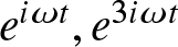 $e^{i \omega t}, e^{3 i \omega t}$ (i.e., we ignore higher-order time harmonics $e^{\pm5i\omega t},e^{\pm7i\omega t},e^{\pm9i\omega t}$). The resulting system is the following approximate, coupled Klein–Gordon system, in the form
 \begin{equation}
\left\{
\begin{matrix}
u_{tt}+2 i \omega u_t - u_{xx}+(4-\omega^2) u -( 6 u^2 \bar{u}+6 \bar{u}^2 v +12 u |v|^2)=0 \\
v_{tt}+6 i \omega v_t-v_{xx}+(4-9 \omega^2) v -(2 u^3+12 |u|^2 v+6 |v|^2 v)=0.
\end{matrix}
\right.
\end{equation}
\begin{equation}
\left\{
\begin{matrix}
u_{tt}+2 i \omega u_t - u_{xx}+(4-\omega^2) u -( 6 u^2 \bar{u}+6 \bar{u}^2 v +12 u |v|^2)=0 \\
v_{tt}+6 i \omega v_t-v_{xx}+(4-9 \omega^2) v -(2 u^3+12 |u|^2 v+6 |v|^2 v)=0.
\end{matrix}
\right.
\end{equation}Here, the relevant Hamiltonian is
 \begin{align}
H[u,v] & = \frac{1}{2}\int \bigg[
|u_x|^2 + |v_x|^2 + |u_t + i\omega u|^2 +
|v_t + 3i\omega v|^2
+ (4-\omega^2)|u|^2 + (4-9\omega^2)|v|^2 \nonumber\\
& \quad +
3|u|^4 + 3u^2\bar{u}\bar{v} + 3\bar{u}^2uv + 6|u|^2|v|^2+
u^3\bar{v} + \bar{u}^3v + 3|v|^4
\bigg] dx\end{align}
\begin{align}
H[u,v] & = \frac{1}{2}\int \bigg[
|u_x|^2 + |v_x|^2 + |u_t + i\omega u|^2 +
|v_t + 3i\omega v|^2
+ (4-\omega^2)|u|^2 + (4-9\omega^2)|v|^2 \nonumber\\
& \quad +
3|u|^4 + 3u^2\bar{u}\bar{v} + 3\bar{u}^2uv + 6|u|^2|v|^2+
u^3\bar{v} + \bar{u}^3v + 3|v|^4
\bigg] dx\end{align} Now, we are interested in time-independentFootnote 1 solutions of this system  $(u,v)=(\phi, \psi)$, which satisfy the elliptic system
 \begin{equation}
\left\{ \begin{matrix}
-\phi''+(4-\omega^2) \phi -
(6\phi^2 \bar{\phi}+6 \bar{\phi}^2 \psi+12 \phi |\psi|^2)=0, \\
-\psi''+(4-9 \omega^2) \psi -(2 \phi^3+12 |\phi|^2\psi +6 |\psi|^2\psi) = 0.
\end{matrix}\right.
\end{equation}
\begin{equation}
\left\{ \begin{matrix}
-\phi''+(4-\omega^2) \phi -
(6\phi^2 \bar{\phi}+6 \bar{\phi}^2 \psi+12 \phi |\psi|^2)=0, \\
-\psi''+(4-9 \omega^2) \psi -(2 \phi^3+12 |\phi|^2\psi +6 |\psi|^2\psi) = 0.
\end{matrix}\right.
\end{equation} We are looking for real-valued solutions  $\phi, \psi$ of (2.6). We define the currents
 \begin{equation*}
J_\phi(x):=\mathrm{Im}(\bar\phi\,\phi'),\qquad
J_\psi(x):=\mathrm{Im}(\bar\psi\,\psi').
\end{equation*}
\begin{equation*}
J_\phi(x):=\mathrm{Im}(\bar\phi\,\phi'),\qquad
J_\psi(x):=\mathrm{Im}(\bar\psi\,\psi').
\end{equation*} A straightforward calculation involving the derivative of such quantities can be used to establish that any single-component stationary solution considered (such as  $(0,\psi)$) will, by necessity, be real, up to an overall constant phase factor. Two-component stationary states can be seen (again, through a direct calculation) to possess the constraint (from Eq. (2.6), for solutions vanishing at infinity)
 \begin{equation}
J_\phi(x)+3J_\psi(x)\equiv 0
\end{equation}
\begin{equation}
J_\phi(x)+3J_\psi(x)\equiv 0
\end{equation}at steady state. Yet, they are not necessarily always real (i.e., possessing a phase that is vanishing up to an overall constant). Nonetheless – and also for reasons that connect non-trivial  $(\phi,\psi)$ waveforms to the full original system of Eq. (2.1) in Section 6 below – here we will only consider real solutions in what follows. As a motivation to that effect, the variational solutions of interest herein (see Proposition 4.1 below) are necessarily real. In this sense, if one is looking for energetically favourable configurations, the real solutions are the only plausible option, per the construction of Proposition 4.1 below. In such a case, the approximate solution (2.3) is in the form
 \begin{equation}
2\left[ \phi\cos(\omega t)+ \psi \cos(3\omega t)\right].
\end{equation}
\begin{equation}
2\left[ \phi\cos(\omega t)+ \psi \cos(3\omega t)\right].
\end{equation} From this point on, our object of interest is the dynamics of the system (2.4), specifically the stability of its stationary solutions  $(\phi, \psi)$ of (2.6).
Theorem 2.1 (Existence of bell-shaped oscillons)
Let 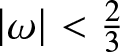 $|\omega| \lt \frac{2}{3}$. Then, the system (2.6) has a solution $(\phi, \psi)$, where both $\phi, \psi$ are real-valued and bell-shaped functions.Footnote 2 In addition, $\phi, \psi$ are smooth and exponentially localized. More specifically,
 \begin{equation*}
\phi(x) \sim e^{-\sqrt{4-\omega^2}|x|}, \ \ \psi(x)\sim e^{-\sqrt{4-9 \omega^2}|x|}, |x| \gt \gt 1.
\end{equation*}
\begin{equation*}
\phi(x) \sim e^{-\sqrt{4-\omega^2}|x|}, \ \ \psi(x)\sim e^{-\sqrt{4-9 \omega^2}|x|}, |x| \gt \gt 1.
\end{equation*} In addition, the associated self-adjoint linearized operator, see Section 2.1 below, has 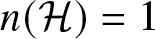 $n(\mathcal{H})=1$.
The proof of Theorem 2.1 is variational in nature, so we postpone it to Section 4. Specifically, we refer to Proposition 4.1 below.
2.1. Linearization around the steady states
Let us now consider the linearized problem associated with the system (2.4). To this end, we adopt the variables
 \begin{equation*}
u=\phi+p+i q, v=\psi+r+i s
\end{equation*}
\begin{equation*}
u=\phi+p+i q, v=\psi+r+i s
\end{equation*}Plugging this ansatz in (2.4), taking real and imaginary parts separate and ignoring all quadratic and higher-order terms leads to
 \begin{equation}
\left\{
\begin{matrix}
p_{tt}-2\omega q_t-p_{xx}+(4-\omega^2) p -[(18 \phi^2+12 \psi^2+12\phi\psi)p+(6 \phi^2+24 \phi\psi)r]=0 \\
q_{tt}+ 2\omega p_t-q_{xx}+(4-\omega^2) q-[(6\phi^2+12\psi^2-12\phi\psi)q+6 \phi^2 s]=0 \\
r_{tt}-6 \omega s_t -r_{xx}+(4-9 \omega^2) r -[(12\phi^2+18 \psi^2)r+(6\phi^2+24 \psi^2) p]=0 \\
s_{tt}+6 \omega r_t-s_{xx} +(4-9\omega^2) s - [6 \phi^2 q +(12\phi^2+6 \psi^2)s]=0.
\end{matrix}
\right.
\end{equation}
\begin{equation}
\left\{
\begin{matrix}
p_{tt}-2\omega q_t-p_{xx}+(4-\omega^2) p -[(18 \phi^2+12 \psi^2+12\phi\psi)p+(6 \phi^2+24 \phi\psi)r]=0 \\
q_{tt}+ 2\omega p_t-q_{xx}+(4-\omega^2) q-[(6\phi^2+12\psi^2-12\phi\psi)q+6 \phi^2 s]=0 \\
r_{tt}-6 \omega s_t -r_{xx}+(4-9 \omega^2) r -[(12\phi^2+18 \psi^2)r+(6\phi^2+24 \psi^2) p]=0 \\
s_{tt}+6 \omega r_t-s_{xx} +(4-9\omega^2) s - [6 \phi^2 q +(12\phi^2+6 \psi^2)s]=0.
\end{matrix}
\right.
\end{equation}This is the form of the linearized problem. We now need to convert this to a more standard, first order in time, eigenvalue problem. This is done in a number of steps.
2.1.1. The eigenvalue problem
In matrix form,
 \begin{equation}
\left(\begin{matrix}
p \\q \\ r\\s
\end{matrix}\right)_{tt}+ \left(\begin{matrix}
0 & -2\omega & 0 & 0 \\
2\omega &0 & 0 & 0 \\
0&0& 0& -6\omega \\
0 & 0 & 6\omega & 0
\end{matrix}\right) \left(\begin{matrix}
p \\q \\ r\\s
\end{matrix}\right)_{t} + \mathcal{H} \left(\begin{matrix}
p \\q \\ r\\s
\end{matrix}\right)=0,
\end{equation}
\begin{equation}
\left(\begin{matrix}
p \\q \\ r\\s
\end{matrix}\right)_{tt}+ \left(\begin{matrix}
0 & -2\omega & 0 & 0 \\
2\omega &0 & 0 & 0 \\
0&0& 0& -6\omega \\
0 & 0 & 6\omega & 0
\end{matrix}\right) \left(\begin{matrix}
p \\q \\ r\\s
\end{matrix}\right)_{t} + \mathcal{H} \left(\begin{matrix}
p \\q \\ r\\s
\end{matrix}\right)=0,
\end{equation}where
 \begin{equation}
\mathcal{H}:=\left(\begin{matrix}
\mathcal{H}_1& 0 & - 24 \phi\psi -6\phi^2 & 0 \\
0 & \mathcal{H}_2 &0 & -6 \phi^2\\
- 24 \phi\psi -6\phi^2 & 0 &\mathcal{H}_3 & 0\\
0 & -6 \phi^2 & 0 & \mathcal{H}_4
\end{matrix}\right)
\end{equation}
\begin{equation}
\mathcal{H}:=\left(\begin{matrix}
\mathcal{H}_1& 0 & - 24 \phi\psi -6\phi^2 & 0 \\
0 & \mathcal{H}_2 &0 & -6 \phi^2\\
- 24 \phi\psi -6\phi^2 & 0 &\mathcal{H}_3 & 0\\
0 & -6 \phi^2 & 0 & \mathcal{H}_4
\end{matrix}\right)
\end{equation}and
 \begin{align*}
\mathcal{H}_1 &= -\partial_{xx}+(4-\omega^2) - 18 \phi^2-12\psi^2- 12 \phi\psi; \ \
\mathcal{H}_2 = -\partial_{xx}+(4-\omega^2) - 6 \phi^2 - 12 \psi^2 +12 \phi\psi \\
\mathcal{H}_3&= -\partial_{xx}+(4-9 \omega^2) -12 \phi^2 - 18 \psi^2; \ \
\mathcal{H}_4 = -\partial_{xx}+(4-9 \omega^2) -12 \phi^2 - 6 \psi^2
\end{align*}
\begin{align*}
\mathcal{H}_1 &= -\partial_{xx}+(4-\omega^2) - 18 \phi^2-12\psi^2- 12 \phi\psi; \ \
\mathcal{H}_2 = -\partial_{xx}+(4-\omega^2) - 6 \phi^2 - 12 \psi^2 +12 \phi\psi \\
\mathcal{H}_3&= -\partial_{xx}+(4-9 \omega^2) -12 \phi^2 - 18 \psi^2; \ \
\mathcal{H}_4 = -\partial_{xx}+(4-9 \omega^2) -12 \phi^2 - 6 \psi^2
\end{align*} Note that the operator  $\mathcal{H}$ is self-adjoint, for nice enough $\phi, \psi$, when taken with the domain $H^2(\mathbb{R})\times H^2(\mathbb{R})\times H^2(\mathbb{R})\times H^2(\mathbb{R})$, while
 \begin{equation*}
\mathcal{J}:=\left(\begin{matrix}
0 & -2\omega & 0 & 0 \\
2\omega &0 & 0 & 0 \\
0&0& 0& -6\omega \\
0 & 0 & 6\omega & 0
\end{matrix}\right) ,
\end{equation*}
\begin{equation*}
\mathcal{J}:=\left(\begin{matrix}
0 & -2\omega & 0 & 0 \\
2\omega &0 & 0 & 0 \\
0&0& 0& -6\omega \\
0 & 0 & 6\omega & 0
\end{matrix}\right) ,
\end{equation*}is skew-symmetric, i.e.,  $\mathcal{J}^*=-\mathcal{J}$. The corresponding eigenvalue problem, which can be obtained by the assignment
 \begin{equation*}
\left(\begin{matrix}
p \\q \\ r\\s
\end{matrix}\right)\to e^{\lambda t} \left(\begin{matrix}
p \\q \\ r\\s
\end{matrix}\right)=:e^{\lambda t}\vec{z}
\end{equation*}
\begin{equation*}
\left(\begin{matrix}
p \\q \\ r\\s
\end{matrix}\right)\to e^{\lambda t} \left(\begin{matrix}
p \\q \\ r\\s
\end{matrix}\right)=:e^{\lambda t}\vec{z}
\end{equation*}can be written in the form
 \begin{equation*}
\lambda^2 \vec{z} +\lambda \mathcal{J} \vec{z}+ \mathcal{H} \vec{z}=0.
\end{equation*}
\begin{equation*}
\lambda^2 \vec{z} +\lambda \mathcal{J} \vec{z}+ \mathcal{H} \vec{z}=0.
\end{equation*}This eigenvalue problem is a pencil of order two, and these have been an object of intense investigations. A standard equivalence in a more classical Hamiltonian form is as followsFootnote 3
 \begin{equation}
\left(\begin{matrix}
0 & -Id \\ Id & -\mathcal{J}
\end{matrix}\right) \left(\begin{matrix}
\mathcal{H} & 0 \\ 0 & I
\end{matrix}\right)
\left(\begin{matrix}
\vec{z} \\ \vec{w}
\end{matrix}\right)= \lambda \left(\begin{matrix}
\vec{z} \\ \vec{w}
\end{matrix}\right)
\end{equation}
\begin{equation}
\left(\begin{matrix}
0 & -Id \\ Id & -\mathcal{J}
\end{matrix}\right) \left(\begin{matrix}
\mathcal{H} & 0 \\ 0 & I
\end{matrix}\right)
\left(\begin{matrix}
\vec{z} \\ \vec{w}
\end{matrix}\right)= \lambda \left(\begin{matrix}
\vec{z} \\ \vec{w}
\end{matrix}\right)
\end{equation}This prompts the following definition.


2.2. Stability of the waves
Next, we address the important issue of symmetries and the corresponding eigenvalues at zero for the linearized problem, that arise.
2.2.1. Symmetries of the system
We can identify at least two symmetries of the system (2.6), namely a translational and (phase) modulational invariance. Specifically, for every solution  $(\phi, \psi)$ of (2.6) and arbitrary real $y$, then $(\phi(\cdot-y), \psi(\cdot-y))$,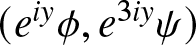 $(e^{i y} \phi, e^{3i y} \psi)$ are solutions as well. The usual differentiation in the parameter $y$, and taking into account the setup of $\mathcal{H}$, provides two elements in $Ker[\mathcal{H}]$. More concretely,
 \begin{equation*}
\left(\begin{matrix}
\phi' \\ 0 \\ \psi'\\ 0
\end{matrix} \right), \ \ \ \left(\begin{matrix}
0 \\ \phi \\ 0 \\ 3 \psi
\end{matrix} \right) \in Ker[\mathcal{H}].
\end{equation*}
\begin{equation*}
\left(\begin{matrix}
\phi' \\ 0 \\ \psi'\\ 0
\end{matrix} \right), \ \ \ \left(\begin{matrix}
0 \\ \phi \\ 0 \\ 3 \psi
\end{matrix} \right) \in Ker[\mathcal{H}].
\end{equation*}2.2.2. Non-degeneracy of the wave pair φ, ψ
We now introduce the notion of a non-degeneracy for the wave pair  $(\phi, \psi)$.
Definition 2.3. We say that the solution  $(\phi, \psi)$ is non-degenerate if there are no more elements of $Ker[\mathcal{H}]$ other than those already found. Specifically,
 \begin{equation*}
Ker[\mathcal{H}] = span \left[\left(\begin{matrix}
\phi' \\ 0 \\ \psi'\\ 0
\end{matrix} \right), \ \ \ \left(\begin{matrix}
0 \\ \phi \\ 0 \\ 3 \psi
\end{matrix} \right) \right]
\end{equation*}
\begin{equation*}
Ker[\mathcal{H}] = span \left[\left(\begin{matrix}
\phi' \\ 0 \\ \psi'\\ 0
\end{matrix} \right), \ \ \ \left(\begin{matrix}
0 \\ \phi \\ 0 \\ 3 \psi
\end{matrix} \right) \right]
\end{equation*} In other words, non-degeneracy means that the only zeros in the kernel of  $\mathcal{H}$ are those generated by the symmetries of the system.
We are now ready to state the main stability result.
Theorem 2.4. Let 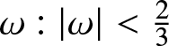 $\omega: |\omega| \lt \frac{2}{3}$. Assume that the steady state solution $(\phi, \psi)$ of (2.4), constructedFootnote 4 in Theorem 2.1, is a non-degenerate, smooth function of $\omega$. That is, the mapping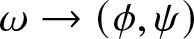 $\omega\to (\phi, \psi)$ is Frechet differentiable.
Then, it is spectrally stable if and only if the following holds true
 \begin{equation*}
\omega \partial_\omega \int_{\mathbb{R}} \left(\phi^2+9 \psi^2\right) dx + \int_{\mathbb{R}} \left(\phi^2+9 \psi^2\right) dx \lt 0.
\end{equation*}
\begin{equation*}
\omega \partial_\omega \int_{\mathbb{R}} \left(\phi^2+9 \psi^2\right) dx + \int_{\mathbb{R}} \left(\phi^2+9 \psi^2\right) dx \lt 0.
\end{equation*} Equivalently,  $\omega\to \omega \int_{\mathbb{R}} \left(\phi^2+9 \psi^2\right) dx$ is decreasing.
3. Preliminaries
We use standard notations for the  $L^p$ spaces, namely with the norm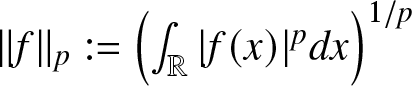 $\|f\|_p:=\left(\int_{\mathbb{R}} |f(x)|^p dx\right)^{1/p}$, and the Sobolev spaces $H^s(\mathbb{R})$. The Sobolev embedding guarantees that for all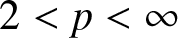 $2 \lt p \lt \infty$, there is a constant $C_p$, so that $\|u\|_p\leq C_p \|u\|_{H^1}$.
3.1. Decreasing rearrangements and compactness criteria
One tool that will be useful in the sequel is the notion of the decreasing rearrangement. For a function 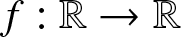 $f:\mathbb{R}\to \mathbb{R}$, there exists an even, positive, non-increasing on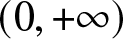 $(0, +\infty)$ function $f^*$, so that the corresponding level functions coincide, i.e.,
  $
d_f(\alpha)=\{x: |f(x)| \gt \alpha\}=\{x: f^*(x) \gt \alpha\}=d_{f^*}(\alpha)
$ Alternatively, a constructive definition may be given as follows
$
d_f(\alpha)=\{x: |f(x)| \gt \alpha\}=\{x: f^*(x) \gt \alpha\}=d_{f^*}(\alpha)
$ Alternatively, a constructive definition may be given as follows
 \begin{equation*}
f^*(t)=\inf\left\{s: d_f(s)\leq 2|t| \right\}, \ \ t\in \mathbb{R}
\end{equation*}
\begin{equation*}
f^*(t)=\inf\left\{s: d_f(s)\leq 2|t| \right\}, \ \ t\in \mathbb{R}
\end{equation*} Either way, we conclude that 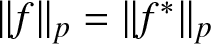 $\|f\|_p=\|f^*\|_p$. Additionally, there are the standard inequalities
 \begin{equation*}
\int_{\mathbb{R}} f(x) g(x) dx\leq \int_{\mathbb{R}} f^*(x) g^*(x) dx, \int_{\mathbb{R}^2} f(x-y) g(y) h(x) dx dy \leq
\int_{\mathbb{R}^2} f^*(x-y) g^*(y) h^*(x) dx dy
\end{equation*}
\begin{equation*}
\int_{\mathbb{R}} f(x) g(x) dx\leq \int_{\mathbb{R}} f^*(x) g^*(x) dx, \int_{\mathbb{R}^2} f(x-y) g(y) h(x) dx dy \leq
\int_{\mathbb{R}^2} f^*(x-y) g^*(y) h^*(x) dx dy
\end{equation*} The Szegö inequality guarantees that 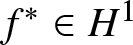 $f^*\in H^1$, whenever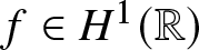 $f\in H^1(\mathbb{R})$ and moreover,
 \begin{equation}
\|\partial_x f\|\geq \|\partial_x f^*\|
\end{equation}
\begin{equation}
\|\partial_x f\|\geq \|\partial_x f^*\|
\end{equation} In case of equality in (3.1), one concludes that the function  $f$ coincides with its rearrangement, i.e.,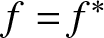 $f=f^*$, and therefore it belongs to a class of functions, usually referred to as bell-shaped.
The Riesz–Relich–Kolmogorov compactness criteria (or rather a consequence thereof) is the following – a sequence  $\{u_n\}_n$ is compact in $L^p(\mathbb{R}), 1 \lt p \lt \infty$, if
• $\sup_n \|u_n\|_{H^1(\mathbb{R})} \lt \infty$
• For every
$\epsilon \gt 0$, there exists
$R=R_\epsilon \gt 0$, so that
\begin{equation*}
\sup_n \int_{|x| \gt R} |u_n(x)|^p dx \lt \epsilon.
\end{equation*}




3.2. Basics of the instability index theory
Consider a Hamiltonian eigenvalue problem in the form
 \begin{equation}
J L u =\lambda u
\end{equation}
\begin{equation}
J L u =\lambda u
\end{equation}where 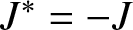 $J^*=-J$ and $L^*=L$, with appropriate domains for the composition operator $J L$. Assume in addition that both $J, L$ act on spaces of functions, and they do preserve real-valued functions. The stability of (3.2) is a fundamental problem in modern dynamics. Specifically, as in Definition 2.2, we say that the problem (3.2) is stable if there are no non-trivial solutions of (3.2) with $\mathrm{Re}\lambda \gt 0$. In order to introduce some relevant notions, we assume that $L$ is semi-bounded from below, that is, there exists a constant $C$, so that $L\geq C$ in the sense of quadratic forms. In fact, we assume that its negative subspace $X_-$ is finite dimensional and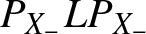 $P_{X_-} L P_{X_-}$ has only point spectrum, each with finite multiplicity. Denote its Morse index by
 \begin{equation*}
n(L)=dim[X_-]=\#\{\sigma: \sigma \lt 0: \sigma \in \sigma_{p.p.}(L)\}.
\end{equation*}
\begin{equation*}
n(L)=dim[X_-]=\#\{\sigma: \sigma \lt 0: \sigma \in \sigma_{p.p.}(L)\}.
\end{equation*} Next, let  $k_r$ be the number of positive eigenvalues of (3.2), $k_c$ be the number of quadruplets of eigenvalues with non-zero real and imaginary parts, and $k_i^-$, the number of pairs of purely imaginary eigenvalues with negative Krein-signature. For a simple pair of imaginary eigenvalues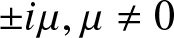 $\pm i \mu, \mu\neq 0$, and the corresponding eigenvector
 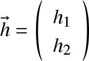 $\vec{h} = \left(\begin{array}{c}
h_1 \\ h_2
\end{array}\right) $, the Krein signature, either
$\vec{h} = \left(\begin{array}{c}
h_1 \\ h_2
\end{array}\right) $, the Krein signature, either  $\pm 1$ is the following quantity
 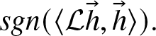 $
sgn(\langle \mathcal{L} \vec{h}, \vec{h} \rangle).
$ Consider the generalized kernel of
$
sgn(\langle \mathcal{L} \vec{h}, \vec{h} \rangle).
$ Consider the generalized kernel of  $J L$
$J L$
 \begin{equation*}
gKer(J L)=span[(Ker(J L)^l, l=1, 2, \ldots] .
\end{equation*}
\begin{equation*}
gKer(J L)=span[(Ker(J L)^l, l=1, 2, \ldots] .
\end{equation*} Assume that  $dim(gKer(J L)) \lt \infty$, although this is, strictly speaking, not required in [Reference Lin and Zeng19]. Select a basis in
 \begin{equation*}
gKer(J L)\ominus Ker(L)=span[\eta_j, j=1, \ldots, N].
\end{equation*}
\begin{equation*}
gKer(J L)\ominus Ker(L)=span[\eta_j, j=1, \ldots, N].
\end{equation*} Introduce  $\mathcal{D}\in \mathcal{M}_{N\times N}$,
 \begin{equation*}
\mathcal{D}:=\{\mathcal{D}_{i j}\}_{i,j=1}^N: \mathcal{D}_{i j}=\langle \mathcal{L} \eta_i, \eta_j \rangle .
\end{equation*}
\begin{equation*}
\mathcal{D}:=\{\mathcal{D}_{i j}\}_{i,j=1}^N: \mathcal{D}_{i j}=\langle \mathcal{L} \eta_i, \eta_j \rangle .
\end{equation*} Then, following [Reference Lin and Zeng19], we have the following formula, relating the number of ‘instabilities’ or Hamiltonian index of the eigenvalue problem (3.2) and the Morse indices of the operators  $L$ and $\mathcal{D}$,
 \begin{equation}
k_{Ham}:=k_r+2 k_c+2k_i^-=n(L)-n(\mathcal{D}).
\end{equation}
\begin{equation}
k_{Ham}:=k_r+2 k_c+2k_i^-=n(L)-n(\mathcal{D}).
\end{equation} Specifically, if  $n(L)=1$, it follows from (3.3) that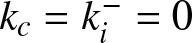 $k_c=k_i^-=0$ and
 \begin{equation}
k_r=1-n(\mathcal{D}).
\end{equation}
\begin{equation}
k_r=1-n(\mathcal{D}).
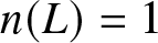
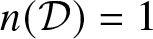
\end{equation} Note that in the case 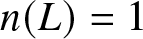 $n(L)=1$, instability occurs exactly when $n(\mathcal{D})=0$, while stability occurs whenever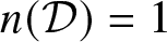 $n(\mathcal{D})=1$. We formulate this in a corollary as follows.
4. Construction of the waves
We can clearly see that the elliptic system (2.6) is of the form
 \begin{equation}
\left\{ \begin{matrix}
-\phi''+(4-\omega^2) \phi -
\frac{\partial F}{\partial \bar{\phi}}=0 \\
-\psi''+(4-9 \omega^2) \psi - \frac{\partial F}{\partial \bar{\psi}}=0
\end{matrix}\right.
\end{equation}
\begin{equation}
\left\{ \begin{matrix}
-\phi''+(4-\omega^2) \phi -
\frac{\partial F}{\partial \bar{\phi}}=0 \\
-\psi''+(4-9 \omega^2) \psi - \frac{\partial F}{\partial \bar{\psi}}=0
\end{matrix}\right.
\end{equation}where
 \begin{equation}
F(u,v,\bar{u}, \bar{v})= 3 |u|^4 +2 \bar{u}^3 v+ 12 |u|^2 |v|^2 +2 u^3 \bar{v}+3 |v|^4=3(|u|^4+|v|^4+4 |u|^2|v|^2)+4 \mathrm{Re} \bar{u}^3 v.
\end{equation}
\begin{equation}
F(u,v,\bar{u}, \bar{v})= 3 |u|^4 +2 \bar{u}^3 v+ 12 |u|^2 |v|^2 +2 u^3 \bar{v}+3 |v|^4=3(|u|^4+|v|^4+4 |u|^2|v|^2)+4 \mathrm{Re} \bar{u}^3 v.
\end{equation}As such, it supports a Hamiltonian structure in the form
 \begin{align}H_1\lbrack\phi,\psi\rbrack & =\frac12\int\left[\vert\phi'\vert^2+\vert\psi'\vert^2+(4-\omega^2)\vert\phi\vert^2+(4-9\omega^2)\vert\psi\vert^2+6(\vert\phi\vert^4+\vert\psi\vert^4+4\vert\phi\vert^2\vert\psi\vert^2)\right.\nonumber \\ & \qquad \left.+8\mathrm{Re}\lbrack\overline\phi^3\psi\rbrack\right]dx\end{align}
 Clearly, one obtains  $H_1[\phi, \psi]=H[z]$ under the transformation (2.8). While here we mention in passing the Hamiltonian structure of the steady state ODEs, naturally, the relevant transformation can also be used to obtain the Hamiltonian structure of the PDEs of the system of Eqs. (2.4).
Proposition 4.1. Let 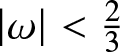 $|\omega| \lt \frac{2}{3}$. Then, the variational problem
 \begin{equation}
\left\{
\begin{matrix}
J[u,v]=\int_{-\infty}^{+\infty}3(|u|^4+|v|^4+4 |u|^2|v|^2)+4 \mathrm{Re}[\bar{u}^3 v]\to \max \\
I[u,v]= \int_{-\infty}^{+\infty} (u')^2+(v')^2+(4-\omega^2)u^2+(4-9\omega^2)v^2 dx=1.
\end{matrix}
\right.
\end{equation}
\begin{equation}
\left\{
\begin{matrix}
J[u,v]=\int_{-\infty}^{+\infty}3(|u|^4+|v|^4+4 |u|^2|v|^2)+4 \mathrm{Re}[\bar{u}^3 v]\to \max \\
I[u,v]= \int_{-\infty}^{+\infty} (u')^2+(v')^2+(4-\omega^2)u^2+(4-9\omega^2)v^2 dx=1.
\end{matrix}
\right.
\end{equation}has a solution  $(U, V)$, with $U\geq 0, V\geq 0$, and $U,V$ are both even. In addition, $(U, V)$ satisfy the Euler–Lagrange equation,
 \begin{equation}
\left\{ \begin{matrix}
-U''+(4-\omega^2) U- \frac{1}{J_0}
(6U^3+12 V^2 U + 6 U^2 V)=0, \\
-V''+(4-9 \omega^2) V -\frac{1}{J_0} (6 V^3+12 U^2 V +2 U^3) = 0,
\end{matrix}\right.
\end{equation}
\begin{equation}
\left\{ \begin{matrix}
-U''+(4-\omega^2) U- \frac{1}{J_0}
(6U^3+12 V^2 U + 6 U^2 V)=0, \\
-V''+(4-9 \omega^2) V -\frac{1}{J_0} (6 V^3+12 U^2 V +2 U^3) = 0,
\end{matrix}\right.
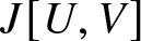
\end{equation}where we denoted  $J_0:=\sup_{I[u,v]=1} J[u,v]=J[U,V]$.
• The solutions
$(\phi, \psi)$ of (4.1) may be obtained as
$\phi=c_0 U, \psi=c_0 V$, where
$c_0$ depends only on
$J[U, V]$, and so on
$\omega$ only.• Intuitively, one expects that for values of
$\omega$, sufficiently close to
$\pm \frac{2}{3}$ we may get the ‘semi-simple’ solution
$U=0, V=C {\rm sech}(\sqrt{4-9 \omega^2}x)$ (for suitably chosen
$C$, so that
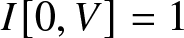
$I[0,V]=1$). Indeed, in the variational problem (4.4), it becomes a viable strategy (as
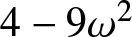
$4-9\omega^2$ becomes small) to ramp up the
$v$ function, and at the same time to drop the
$u$ function (which uses substantial
$L^2$ constraint, relative to
$v$). We check numerically, see Figure 3 below, that this indeed happens for values of
$\omega: 0.5316 \lt \omega \lt 2/3$.










Proof. The proof is rather straightforward. To this end, note that by Sobolev embedding  $\|u\|_4\leq C\|u\|_{H^1}$. Estimating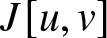 $J[u,v]$ by Hölder’s, we see that
 \begin{equation*}
J[u,v]\leq C (\|u\|^4_4+\|v\|^4_4)\leq C \|u\|^4_{H^1}+\|v\|^4_{H^1})\leq C I^2[u,v].
\end{equation*}
\begin{equation*}
J[u,v]\leq C (\|u\|^4_4+\|v\|^4_4)\leq C \|u\|^4_{H^1}+\|v\|^4_{H^1})\leq C I^2[u,v].
\end{equation*} It follows that 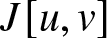 $J[u,v]$ is bounded from above when $u,v$ are under the constraint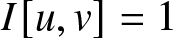 $I[u,v]=1$. Moreover, by elementary properties of the decreasing rearrangements, we have that
 \begin{align*}
J[u,v] &= \int_{-\infty}^{+\infty}3(|u|^4+|v|^4+4 |u|^2|v|^2)+4 \ \mathrm{Re} [\bar{u}^3v]\\
&\leq \int_{-\infty}^{+\infty}3(|u^*|^4+|v^*|^4+4 |u^*|^2|v^*|^2)+4 (u^*)^3 v^* =J[u^*, v^*].
\end{align*}
\begin{align*}
J[u,v] &= \int_{-\infty}^{+\infty}3(|u|^4+|v|^4+4 |u|^2|v|^2)+4 \ \mathrm{Re} [\bar{u}^3v]\\
&\leq \int_{-\infty}^{+\infty}3(|u^*|^4+|v^*|^4+4 |u^*|^2|v^*|^2)+4 (u^*)^3 v^* =J[u^*, v^*].
\end{align*}In terms of the constraints, using the Szegö inequality, we have
 \begin{equation*}
I[u, v]\geq I[u^*, v^*].
\end{equation*}
\begin{equation*}
I[u, v]\geq I[u^*, v^*].
\end{equation*} Assuming for a moment that there holds the strict inequality,  $1=I[u, v] \gt I[u^*, v^*]$, say $I[u^*, v^*]=a \lt 1$, we arrive at a contradiction, since then $u^*, v^*$ satisfy
 \begin{equation*}
\left\{
\begin{matrix}
J[u^*,v^*]\geq J[u, v] \\
I[u^*, v^*]=a \lt 1
\end{matrix}
\right.
\end{equation*}
\begin{equation*}
\left\{
\begin{matrix}
J[u^*,v^*]\geq J[u, v] \\
I[u^*, v^*]=a \lt 1
\end{matrix}
\right.
\end{equation*} But since the problem is scale invariant, we have that  $I[a^{-1/2} u^*, a^{-1/2} v^*]=1$ satisfy the original constraint, while
 \begin{equation*}
J[a^{-1/2} u^*,a^{-1/2} v^*]=a^{-2} J[u^*, v^*]\geq a^{-2} J[u, v] \gt J[u,v],
\end{equation*}
\begin{equation*}
J[a^{-1/2} u^*,a^{-1/2} v^*]=a^{-2} J[u^*, v^*]\geq a^{-2} J[u, v] \gt J[u,v],
\end{equation*}in clear contradiction with the setup of the variational problem (4.4). So,  $I[u, v]=I[u^*, v^*]$, whence it follows that $u=u^*, v=v^*$, i.e., the variational problem may be taken to maximize $J$ only on the set of bell-shaped functions. Using the properties of the bell-shaped functions, and the constraint we have that
 \begin{equation*}
u^2(x)\leq \frac{1}{2x} \int_{-x}^{x} u^2(y) dy\leq \frac{1}{2x} \|u\|^2\leq \frac{C_\omega}{x},
\end{equation*}
\begin{equation*}
u^2(x)\leq \frac{1}{2x} \int_{-x}^{x} u^2(y) dy\leq \frac{1}{2x} \|u\|^2\leq \frac{C_\omega}{x},
\end{equation*}and similar for  $v$. It follows that, for every $R \gt 0$,
 \begin{equation*}
\int_{|x| \gt R} u^4(x) dx\leq C \int_{|x| \gt R} x^{-2} dx \leq C R^{-1},
\end{equation*}
\begin{equation*}
\int_{|x| \gt R} u^4(x) dx\leq C \int_{|x| \gt R} x^{-2} dx \leq C R^{-1},
\end{equation*}and similar for  $v$. This, together with the constraint $\|u\|_{H^1}+\|v\|_{H^1}\leq C$, implies by the Riesz–Kolmogorov criteria, that any maximizing sequence for (4.4) is in fact compact in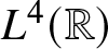 $L^4(\mathbb{R})$. Thus, starting with a maximizing sequence for (4.4), i.e.,
 \begin{equation*}
I[u_n, v_n]=1, J[u_n, v_n]\to \sup_{I[u,v]=1} J[u,v]
\end{equation*}
\begin{equation*}
I[u_n, v_n]=1, J[u_n, v_n]\to \sup_{I[u,v]=1} J[u,v]
\end{equation*}and after taking a strongly convergent in  $L^4$, subsequence $\lim_n \|u_n-U\|_4=0, \lim_n \|v_n-V\|_4=0$, whence
 \begin{equation*}
\lim_n J[u_n,v_n]=J[U,V].
\end{equation*}
\begin{equation*}
\lim_n J[u_n,v_n]=J[U,V].
\end{equation*} At the same time, by the lower semi-continuity of the  $H^1$ norms (with respect to weak convergence, so certainly with respect to $L^4$ convergence),
 \begin{equation*}
I[U, V]\leq \liminf_n I[u_n, v_n]=1.
\end{equation*}
\begin{equation*}
I[U, V]\leq \liminf_n I[u_n, v_n]=1.
\end{equation*} If in fact, we assume that  $I[U,V] \lt 1$, we obtain the same contradiction as above (the value of $\sup_{I[u,v]=1} J[u,v]$ is bigger than it can possibly be), so it follows that $I[U,V]=1$ (and in fact, one may conclude from this that even stronger convergence holds, namely $\lim_n \|u_n-U\|_{H^1}=0, \lim_n \|v_n-V\|_{H^1}=0$). This concludes the proof.
We now derive the Euler–Lagrange equations. To this end, consider testing (4.4) on the pair  $U+\epsilon h_1, V+\epsilon h_2$ for some test functions $h_1, h_2$. Due to the fact that the pair $(U,V)$ is a minimizer, we have that the following scalar function achieves a maximum at $\epsilon=0$,
 \begin{equation*}
g(\epsilon)=\frac{J[U+\epsilon h_1, V+\epsilon h_2]}{I^2[U+\epsilon h_1, V+\epsilon h_2]}
\end{equation*}
\begin{equation*}
g(\epsilon)=\frac{J[U+\epsilon h_1, V+\epsilon h_2]}{I^2[U+\epsilon h_1, V+\epsilon h_2]}
\end{equation*} It follows that  $g'(0)=0$, while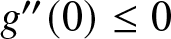 $g''(0)\leq 0$. Note $J_0 \gt 0$. We have
 \begin{align*}
J[U+\epsilon h_1, V+\epsilon h_2]& = J_0+ \epsilon(12\langle U^3, h_1 \rangle+12\langle V^3, h_2 \rangle+24\langle V^2 U, h_1 \rangle\nonumber\\
& \quad +24\langle U^2V, h_2 \rangle+12\langle U^2V, h_1 \rangle+4\langle U^3, h_2 \rangle)+O(\epsilon^2)I^2[U+\epsilon h_1, V+\epsilon h_2]\nonumber\\
& = 1+ 2\epsilon(\langle -U''+(4-\omega^2)U, h_1 \rangle+\langle -V''+(4-\omega^2)V, h_2 \rangle)+O(\epsilon^2).
\end{align*}
\begin{align*}
J[U+\epsilon h_1, V+\epsilon h_2]& = J_0+ \epsilon(12\langle U^3, h_1 \rangle+12\langle V^3, h_2 \rangle+24\langle V^2 U, h_1 \rangle\nonumber\\
& \quad +24\langle U^2V, h_2 \rangle+12\langle U^2V, h_1 \rangle+4\langle U^3, h_2 \rangle)+O(\epsilon^2)I^2[U+\epsilon h_1, V+\epsilon h_2]\nonumber\\
& = 1+ 2\epsilon(\langle -U''+(4-\omega^2)U, h_1 \rangle+\langle -V''+(4-\omega^2)V, h_2 \rangle)+O(\epsilon^2).
\end{align*} Writing out the first order in  $\epsilon$ terms, arising in $g(\epsilon)$, leads to the formulas
 \begin{eqnarray*}
& 12\langle U^3, h_1 \rangle+12\langle V^3, h_2 \rangle+24\langle V^2 U, h_1 \rangle+24\langle U^2V, h_2 \rangle+12\langle U^2V, h_1 \rangle+4\langle U^3, h_2 \rangle \nonumber\\
& \quad = 2 J_0(\langle -U''+(4-\omega^2)U, h_1 \rangle+\langle -V''+(4-\omega^2)V, h_2 \rangle).
\end{eqnarray*}
\begin{eqnarray*}
& 12\langle U^3, h_1 \rangle+12\langle V^3, h_2 \rangle+24\langle V^2 U, h_1 \rangle+24\langle U^2V, h_2 \rangle+12\langle U^2V, h_1 \rangle+4\langle U^3, h_2 \rangle \nonumber\\
& \quad = 2 J_0(\langle -U''+(4-\omega^2)U, h_1 \rangle+\langle -V''+(4-\omega^2)V, h_2 \rangle).
\end{eqnarray*} Since  $h_1, h_2$ are independent increments, we have that $U,V$ are weak solutions of the elliptic system (4.5). Standard elliptic estimates for (4.5) imply that such solutions are in fact $H^\infty(\mathbb{R})$, so in particular, $U,V$ are $C^\infty(\mathbb{R})$ functions. In addition, the large $x$ asymptotics for $U,V$ are as follows
 \begin{equation*}
U(x)\sim e^{-\sqrt{4-\omega^2}|x|}, V(x)\sim e^{-\sqrt{4-9 \omega^2}|x|}.
\end{equation*}
\begin{equation*}
U(x)\sim e^{-\sqrt{4-\omega^2}|x|}, V(x)\sim e^{-\sqrt{4-9 \omega^2}|x|}.
\end{equation*} We now pass to the second-order expansion, in terms of  $\epsilon$, for the function $g$. To simplify matters, we work with the additional restriction that the increments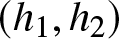 $(h_1, h_2)$ satisfy the constraint,
 \begin{equation}
\mathrm{Re} [\langle -U''+(4-\omega^2)U, h_1 \rangle+\langle -V''+(4-\omega^2)V, h_2 \rangle]=0.
\end{equation}
\begin{equation}
\mathrm{Re} [\langle -U''+(4-\omega^2)U, h_1 \rangle+\langle -V''+(4-\omega^2)V, h_2 \rangle]=0.
\end{equation}As a consequence of this extra property, we have that
 \begin{equation}
I^2[U+\epsilon h_1, V+\epsilon h_2] = 1+ \epsilon^2(\|h_1'\|^2+\|h'_2\|^2+(4-\omega^2) \|h_1\|^2+(4-9\omega^2) \|h_2\|^2).
\end{equation}
\begin{equation}
I^2[U+\epsilon h_1, V+\epsilon h_2] = 1+ \epsilon^2(\|h_1'\|^2+\|h'_2\|^2+(4-\omega^2) \|h_1\|^2+(4-9\omega^2) \|h_2\|^2).
\end{equation} Next, we find the second-order expansion, in terms of  $\epsilon$, for the functional $J[U+\epsilon h_1, V+\epsilon h_2]$. We have
 \begin{equation*}
J[U+\epsilon h_1, V+\epsilon h_2] = J_0+\epsilon (A_1[h_1]+A_2[h_2]+A_3[\bar{h}_1]+A_4[\bar{h}_2])+ \epsilon^2 B[h_1, h_2, \bar{h}_1, \bar{h}_2]+O(\epsilon^3),
\end{equation*}
\begin{equation*}
J[U+\epsilon h_1, V+\epsilon h_2] = J_0+\epsilon (A_1[h_1]+A_2[h_2]+A_3[\bar{h}_1]+A_4[\bar{h}_2])+ \epsilon^2 B[h_1, h_2, \bar{h}_1, \bar{h}_2]+O(\epsilon^3),
\end{equation*}where  $A_1, \ldots, A_4$ are linear forms,Footnote 5 while
 \begin{align*}
B[h_1, h_2, \bar{h}_1, \bar{h}_2] &= \int\left( 12 U^2 h_1\bar{h}_1 + 3 U^2(h_1^2+\bar{h}_1^2) + 12 V^2 h_2\bar{h}_2 + 3 V^2(h_2^2+\bar{h}_2^2)\right) \\
& \quad + \int \left(12 U V (h_1+\bar{h}_1)(h_2+\bar{h}_2)+12 U^2 h_2\bar{h}_2+ 12 V^2 h_1\bar{h}_1\right) \\
& \quad + \int \left( 6 U^2 (\bar{h}_1 h_2+\bar{h}_2 h_1)+6 U V (\bar{h}_1^2+h_1^2)\right).
\end{align*}
\begin{align*}
B[h_1, h_2, \bar{h}_1, \bar{h}_2] &= \int\left( 12 U^2 h_1\bar{h}_1 + 3 U^2(h_1^2+\bar{h}_1^2) + 12 V^2 h_2\bar{h}_2 + 3 V^2(h_2^2+\bar{h}_2^2)\right) \\
& \quad + \int \left(12 U V (h_1+\bar{h}_1)(h_2+\bar{h}_2)+12 U^2 h_2\bar{h}_2+ 12 V^2 h_1\bar{h}_1\right) \\
& \quad + \int \left( 6 U^2 (\bar{h}_1 h_2+\bar{h}_2 h_1)+6 U V (\bar{h}_1^2+h_1^2)\right).
\end{align*} As a consequence of the expansion for  $B$ and (4.7), we have that
 \begin{equation}
0\geq g''(0)= 2(B[h_1, h_2, \bar{h}_1, \bar{h}_2]-J_0 (\|h_1'\|^2+\|h'_2\|^2+(4-\omega^2) \|h_1\|^2+(4-9\omega^2) \|h_2\|^2).
\end{equation}
\begin{equation}
0\geq g''(0)= 2(B[h_1, h_2, \bar{h}_1, \bar{h}_2]-J_0 (\|h_1'\|^2+\|h'_2\|^2+(4-\omega^2) \|h_1\|^2+(4-9\omega^2) \|h_2\|^2).
\end{equation} It is technically more convenient to pass to the new variables  $h_1=p+i q, h_2=r+ i s$, so that we can rewrite (4.8) as follows
 \begin{align*}& \|p'\|^2+\|q'\|^2+\|r'\|^2+\|s'\|^2+(4-\omega^2)(\|p\|^2+\|q\|^2)+(4-9 \omega^2)(\|r\|^2+\|s\|^2) \nonumber\\
& \quad \geq \frac{1}{J_0} \int\left( 12 U^2 (p^2+q^2) +6 U^2(p^2-q^2) + 12 V^2 (r^2+s^2) +6 V^2(r^2-s^2)\right) \nonumber\\
& \qquad + \frac{12}{J_0} \int \left(4 U V p r + U^2 (r^2+s^2)+ V^2(p^2+q^2) \right) \nonumber\\
& \qquad + \frac{12}{J_0} \int \left( U^2 (p r +q s)+ U V (p^2-q^2)\right).
\end{align*}
\begin{align*}& \|p'\|^2+\|q'\|^2+\|r'\|^2+\|s'\|^2+(4-\omega^2)(\|p\|^2+\|q\|^2)+(4-9 \omega^2)(\|r\|^2+\|s\|^2) \nonumber\\
& \quad \geq \frac{1}{J_0} \int\left( 12 U^2 (p^2+q^2) +6 U^2(p^2-q^2) + 12 V^2 (r^2+s^2) +6 V^2(r^2-s^2)\right) \nonumber\\
& \qquad + \frac{12}{J_0} \int \left(4 U V p r + U^2 (r^2+s^2)+ V^2(p^2+q^2) \right) \nonumber\\
& \qquad + \frac{12}{J_0} \int \left( U^2 (p r +q s)+ U V (p^2-q^2)\right).
\end{align*} This last inequality should hold for all increments  $(p+i q, r+i s)$ satisfying (4.6), which is equivalent to
 \begin{equation}
\left(\begin{matrix}
p \\ q \\ r \\s
\end{matrix}\right)\perp \left(\begin{matrix}
- U''+(4-\omega^2) U \\0 \\ - V''+(4-9 \omega^2) V \\ 0
\end{matrix}\right)
\end{equation}
\begin{equation}
\left(\begin{matrix}
p \\ q \\ r \\s
\end{matrix}\right)\perp \left(\begin{matrix}
- U''+(4-\omega^2) U \\0 \\ - V''+(4-9 \omega^2) V \\ 0
\end{matrix}\right)
\end{equation} The condition 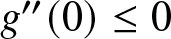 $g''(0)\leq 0$ may be expressed equivalently as the positivity of the following self-adjoint operator, on the co-dimension one subspace described by (4.9),
 \begin{equation*}
\mathcal{L}:=\left(\begin{matrix}
\mathcal{L}_1& 0 & - \frac{24}{J_0} UV -\frac{6}{J_0} U^2 & 0 \\
0 & \mathcal{L}_2 &0 & -\frac{6}{J_0} U^2\\
- \frac{24}{J_0} UV -\frac{6}{J_0} U^2 & 0 &\mathcal{L}_3 & 0\\
0 & -\frac{6}{J_0} U^2 & 0 & \mathcal{L}_4
\end{matrix}\right)
\end{equation*}
\begin{equation*}
\mathcal{L}:=\left(\begin{matrix}
\mathcal{L}_1& 0 & - \frac{24}{J_0} UV -\frac{6}{J_0} U^2 & 0 \\
0 & \mathcal{L}_2 &0 & -\frac{6}{J_0} U^2\\
- \frac{24}{J_0} UV -\frac{6}{J_0} U^2 & 0 &\mathcal{L}_3 & 0\\
0 & -\frac{6}{J_0} U^2 & 0 & \mathcal{L}_4
\end{matrix}\right)
\end{equation*}where
 \begin{align*}
\mathcal{L}_1:&\!= -\partial_{xx}+(4-\omega^2) - \frac{18}{J_0} U^2-\frac{12}{J_0} V^2-\frac{12}{J_0} UV \\
\mathcal{L}_2:&\!= -\partial_{xx}+(4-\omega^2) - \frac{6}{J_0} U^2-\frac{12}{J_0} V^2+\frac{12}{J_0} UV \\
\mathcal{L}_3:&\!= -\partial_{xx}+(4-9 \omega^2) - \frac{18}{J_0} V^2-\frac{12}{J_0} U^2 \\
\mathcal{L}_4:&\!= -\partial_{xx}+(4-9 \omega^2) - \frac{6}{J_0} V^2-\frac{12}{J_0} U^2
\end{align*}
\begin{align*}
\mathcal{L}_1:&\!= -\partial_{xx}+(4-\omega^2) - \frac{18}{J_0} U^2-\frac{12}{J_0} V^2-\frac{12}{J_0} UV \\
\mathcal{L}_2:&\!= -\partial_{xx}+(4-\omega^2) - \frac{6}{J_0} U^2-\frac{12}{J_0} V^2+\frac{12}{J_0} UV \\
\mathcal{L}_3:&\!= -\partial_{xx}+(4-9 \omega^2) - \frac{18}{J_0} V^2-\frac{12}{J_0} U^2 \\
\mathcal{L}_4:&\!= -\partial_{xx}+(4-9 \omega^2) - \frac{6}{J_0} V^2-\frac{12}{J_0} U^2
\end{align*}Clearly, the assignment
 \begin{equation}
\phi:=\frac{U}{\sqrt{J_0}}, \psi:=\frac{V}{\sqrt{J_0}}
\end{equation}
\begin{equation}
\phi:=\frac{U}{\sqrt{J_0}}, \psi:=\frac{V}{\sqrt{J_0}}
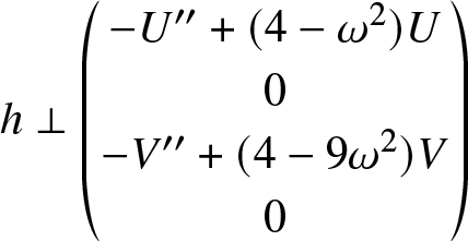
\end{equation}produces bell-shaped solutions of (2.6); moreover, one can infer spectral properties of the corresponding operator from the properties of the operator  $\mathcal{L}$. In fact, we have established more, namely that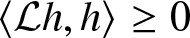 $\langle \mathcal{L} h, h \rangle\geq 0$, whenever
  $h\perp \left(\begin{matrix}
- U''+(4-\omega^2) U \\0 \\ - V''+(4-9 \omega^2) V \\ 0
\end{matrix}\right)$. Using the rescaling transformation (4.10), this is equivalent to
$h\perp \left(\begin{matrix}
- U''+(4-\omega^2) U \\0 \\ - V''+(4-9 \omega^2) V \\ 0
\end{matrix}\right)$. Using the rescaling transformation (4.10), this is equivalent to
 \begin{equation}
\langle \mathcal{H} u, u \rangle\geq 0, u\perp \left(\begin{matrix}
- \phi''+(4-\omega^2) \phi \\0 \\ - \psi''+(4-9 \omega^2) \psi \\ 0
\end{matrix}\right)
\end{equation}
\begin{equation}
\langle \mathcal{H} u, u \rangle\geq 0, u\perp \left(\begin{matrix}
- \phi''+(4-\omega^2) \phi \\0 \\ - \psi''+(4-9 \omega^2) \psi \\ 0
\end{matrix}\right)
\end{equation}We state the results in the following corollary.
Corollary 4.2. The linearized self-adjoint operator  $\mathcal{H}$, introduced in (2.11), has exactly one negative eigenvalue, i.e., the property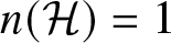 $n(\mathcal{H})=1$.
5. Stability of the waves
In this section, we consider the eigenvalue problem (2.12). Since the self-adjoint portion of it has the property
 \begin{equation*}
n\left(\begin{matrix}
\mathcal{H} & 0 \\ 0 & I
\end{matrix}\right)=n(\mathcal{H})=1,
\end{equation*}
\begin{equation*}
n\left(\begin{matrix}
\mathcal{H} & 0 \\ 0 & I
\end{matrix}\right)=n(\mathcal{H})=1,
\end{equation*}according to Corollary 4.2, we can apply the formula (3.4). To this end, we need to calculate the generalized kernel  $gKer ( \left(\begin{matrix}
0 & -I \\ I & -\mathcal{J}
\end{matrix}
\right) \left(\begin{matrix}
\mathcal{H} & 0 \\ 0 & I
\end{matrix}\right))$, compute the matrix
$gKer ( \left(\begin{matrix}
0 & -I \\ I & -\mathcal{J}
\end{matrix}
\right) \left(\begin{matrix}
\mathcal{H} & 0 \\ 0 & I
\end{matrix}\right))$, compute the matrix  $\mathcal{D}$ and then $n(\mathcal{D})$.
It is actually easy to see that for this program, we may as well restrict our attention to the subspace of even functions. Indeed, the eigenvalue problem (2.12) splits into two independent eigenvalue problems, posed on the even and odd subspaces. The problem with the odd subspace is in fact a trivial one (i.e., no non-trivial solutions). This can be seen from (4.11), as  $\mathcal{H}$ restricted to the odd subspace is in fact a positive operator, i.e.,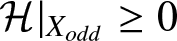 $\mathcal{H}|_{X_{odd}}\geq 0$. Indeed, as $\phi, \psi$ are even functions
 \begin{equation*}
X_{odd}\perp \left(\begin{matrix}
- \phi''+(4-\omega^2) \phi \\0 \\ - \psi''+(4-9 \omega^2) \psi \\ 0
\end{matrix}\right),
\end{equation*}
\begin{equation*}
X_{odd}\perp \left(\begin{matrix}
- \phi''+(4-\omega^2) \phi \\0 \\ - \psi''+(4-9 \omega^2) \psi \\ 0
\end{matrix}\right),
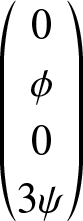
\end{equation*}and hence  $\mathcal{H}|_{X_{odd}}\geq 0$. So, now we proceed to find the adjoint eigenvectors corresponding to the kernel vector
  $\left(\begin{matrix}
0 \\ \phi \\ 0 \\ 3 \psi
\end{matrix} \right) $. We solve
$\left(\begin{matrix}
0 \\ \phi \\ 0 \\ 3 \psi
\end{matrix} \right) $. We solve
 \begin{equation*}
\left(\begin{matrix}
0 & -I \\ I & -\mathcal{J}
\end{matrix}
\right) \left(\begin{matrix}
\mathcal{H} & 0 \\ 0 & I
\end{matrix}\right) \vec{\eta}=\left(\begin{matrix}
0 \\ \phi \\ 0 \\ 3 \psi
\\ 0 \\ 0 \\ 0 \\ 0
\end{matrix} \right).
\end{equation*}
\begin{equation*}
\left(\begin{matrix}
0 & -I \\ I & -\mathcal{J}
\end{matrix}
\right) \left(\begin{matrix}
\mathcal{H} & 0 \\ 0 & I
\end{matrix}\right) \vec{\eta}=\left(\begin{matrix}
0 \\ \phi \\ 0 \\ 3 \psi
\\ 0 \\ 0 \\ 0 \\ 0
\end{matrix} \right).
\end{equation*} Applying the inverse operator  $\left(\begin{matrix}
-\mathcal{J} & I \\ -I & 0
\end{matrix}
\right) $ we obtain for
$\left(\begin{matrix}
-\mathcal{J} & I \\ -I & 0
\end{matrix}
\right) $ we obtain for 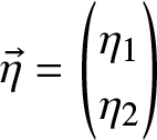 $\vec{\eta}=\left(\begin{matrix} \eta_1 \\ \eta_2 \end{matrix} \right)$,
 \begin{equation*}
\eta_2= -\left(\begin{matrix}
0 \\ \phi \\ 0 \\ 3 \psi
\end{matrix} \right), \mathcal{H} \eta_1=-\mathcal{J} \left(\begin{matrix}
0 \\ \phi \\ 0 \\ 3 \psi
\end{matrix} \right)= 2\omega \left(\begin{matrix}
\phi \\ 0 \\ 9 \psi \\ 0
\end{matrix} \right).
\end{equation*}
\begin{equation*}
\eta_2= -\left(\begin{matrix}
0 \\ \phi \\ 0 \\ 3 \psi
\end{matrix} \right), \mathcal{H} \eta_1=-\mathcal{J} \left(\begin{matrix}
0 \\ \phi \\ 0 \\ 3 \psi
\end{matrix} \right)= 2\omega \left(\begin{matrix}
\phi \\ 0 \\ 9 \psi \\ 0
\end{matrix} \right).
\end{equation*} Taking the derivative with respect to  $\omega$ in the profile equation (2.6) leads to the formula
 \begin{equation}
\mathcal{H} [\partial_\omega \left(\begin{matrix}
\phi \\ 0 \\ \psi \\ 0
\end{matrix} \right)]= 2\omega \left(\begin{matrix}
\phi \\ 0 \\ 9 \psi \\ 0
\end{matrix} \right).
\end{equation}
\begin{equation}
\mathcal{H} [\partial_\omega \left(\begin{matrix}
\phi \\ 0 \\ \psi \\ 0
\end{matrix} \right)]= 2\omega \left(\begin{matrix}
\phi \\ 0 \\ 9 \psi \\ 0
\end{matrix} \right).
\end{equation}Thus, we can take
 \begin{equation*}
\eta_1=\mathcal{H}^{-1}[2\omega \left(\begin{matrix}
\phi \\ 0 \\ 9 \psi \\ 0
\end{matrix} \right)]=\partial_\omega \left(\begin{matrix}
\phi \\ 0 \\ \psi \\ 0
\end{matrix} \right).
\end{equation*}
\begin{equation*}
\eta_1=\mathcal{H}^{-1}[2\omega \left(\begin{matrix}
\phi \\ 0 \\ 9 \psi \\ 0
\end{matrix} \right)]=\partial_\omega \left(\begin{matrix}
\phi \\ 0 \\ \psi \\ 0
\end{matrix} \right).
\end{equation*} In this fashion, we have identified an element 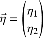 $\vec{\eta}=\left(\begin{matrix} \eta_1 \\ \eta_2 \end{matrix} \right)$ of the generalized kernel, namely
 \begin{equation*}
\eta_1= \partial_\omega \left(\begin{matrix}
\phi \\ 0 \\ \psi \\ 0
\end{matrix} \right), \ \ \eta_2= -\left(\begin{matrix}
0 \\ \phi \\ 0 \\ 3 \psi
\end{matrix} \right).
\end{equation*}
\begin{equation*}
\eta_1= \partial_\omega \left(\begin{matrix}
\phi \\ 0 \\ \psi \\ 0
\end{matrix} \right), \ \ \eta_2= -\left(\begin{matrix}
0 \\ \phi \\ 0 \\ 3 \psi
\end{matrix} \right).
\end{equation*} Proceeding to find further elements of  $gKer$, we need to solve
 \begin{equation*}
\left(\begin{matrix}
0 & -I \\ I & -\mathcal{J}
\end{matrix}
\right) \left(\begin{matrix}
\mathcal{H} & 0 \\ 0 & I
\end{matrix}\right) \vec{z}=\vec{\eta}
\end{equation*}
\begin{equation*}
\left(\begin{matrix}
0 & -I \\ I & -\mathcal{J}
\end{matrix}
\right) \left(\begin{matrix}
\mathcal{H} & 0 \\ 0 & I
\end{matrix}\right) \vec{z}=\vec{\eta}
\end{equation*}Applying the inverse again, we are led to the following system
 \begin{equation*}
\mathcal{H} z_1=-\mathcal{J} \eta_1+\eta_2, \ \ z_2=-\eta_1.
\end{equation*}
\begin{equation*}
\mathcal{H} z_1=-\mathcal{J} \eta_1+\eta_2, \ \ z_2=-\eta_1.
\end{equation*}This of course requires a solvability condition in the first component, namely
 \begin{equation}
-\mathcal{J} \eta_1+\eta_2\perp Ker[\mathcal{H}]=span [\left(\begin{matrix}
0 \\ \phi \\ 0 \\ 3 \psi
\end{matrix} \right)].
\end{equation}
\begin{equation}
-\mathcal{J} \eta_1+\eta_2\perp Ker[\mathcal{H}]=span [\left(\begin{matrix}
0 \\ \phi \\ 0 \\ 3 \psi
\end{matrix} \right)].
\end{equation} Equivalently, the second adjoint eigenvector  $\vec{z}$ does not exist whenever the solvability condition (5.2) is violated. More precisely,
 \begin{equation}0\neq\langle-\mathcal J\eta_1+\eta_2,\begin{pmatrix}0\\\phi\\0\\3\psi\end{pmatrix}\rangle=-\left(\omega\partial_\omega\left(\int\left(\phi^2+9\psi^2\right)dx\right)+\int\left(\phi^2+9\psi^2\right)dx\right)\end{equation}
 Under the condition (5.3), we have that  $dim(gKer)=1$, and hence the matrix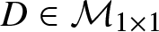 $D\in\mathcal{M}_{1\times 1}$, with
 \begin{equation*}
\mathcal{D}_{11}= \langle \left(\begin{matrix}
\mathcal{H} & 0 \\ 0 & I
\end{matrix}\right)\vec{\eta}, \vec{\eta} \rangle= \langle \mathcal{H} \eta_1, \eta_1 \rangle+\langle \eta_2, \eta_2 \rangle=\omega\partial_\omega
\int_{\mathbb{R}} \left(\phi^2+9 \psi^2\right) dx + \int_{\mathbb{R}} \left(\phi^2+9 \psi^2\right) dx
\end{equation*}
\begin{equation*}
\mathcal{D}_{11}= \langle \left(\begin{matrix}
\mathcal{H} & 0 \\ 0 & I
\end{matrix}\right)\vec{\eta}, \vec{\eta} \rangle= \langle \mathcal{H} \eta_1, \eta_1 \rangle+\langle \eta_2, \eta_2 \rangle=\omega\partial_\omega
\int_{\mathbb{R}} \left(\phi^2+9 \psi^2\right) dx + \int_{\mathbb{R}} \left(\phi^2+9 \psi^2\right) dx
\end{equation*} Thus, according to the index counting theory, more precisely (3.4), the waves are stable in the case of 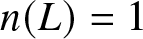 $n(L)=1$, if and only if
 \begin{equation}
\partial_\omega\left(\omega \int_{\mathbb{R}} \left(\phi^2+9 \psi^2\right) dx \right)=\omega \partial_\omega \int_{\mathbb{R}} \left(\phi^2+9 \psi^2\right) dx +\int_{\mathbb{R}} \left(\phi^2+9 \psi^2\right) dx \lt 0
\end{equation}
\begin{equation}
\partial_\omega\left(\omega \int_{\mathbb{R}} \left(\phi^2+9 \psi^2\right) dx \right)=\omega \partial_\omega \int_{\mathbb{R}} \left(\phi^2+9 \psi^2\right) dx +\int_{\mathbb{R}} \left(\phi^2+9 \psi^2\right) dx \lt 0
\end{equation}Equivalently, in this case, the stability is equivalent to the property that
 \begin{equation*}
\omega\to \omega \int_{\mathbb{R}} \left(\phi^2+9 \psi^2\right) dx
\end{equation*}
\begin{equation*}
\omega\to \omega \int_{\mathbb{R}} \left(\phi^2+9 \psi^2\right) dx
\end{equation*}is a decreasing function.
In what follows, we will explore the different branches of the real solutions of Eqs. (2.6), which can be used according to the prescription of Eq. (2.3) in order to develop approximations to the oscillon periodic orbits of Eq. (2.1). We will subsequently study the stability of these states at the level of the reduced equations (2.4) and will then seek to connect the resulting conclusions with the original PDE of Eq. (2.1).
6. Numerical results
6.1. Numerical oscillons
In our efforts to identify solutions to Eqs. (2.6), we found three branches of possible solutions. We thus hereafter explore these solution branches that can be discerned in the diagrams of the left panel of Figure 1. This is complemented by an example of the profile of each of the oscillon branches that we have identified in the right panel of the figure. The former represents the amplitude of the  $\phi(x)$ component, providing a useful bifurcation diagnostic accordingly. For completeness, we also show the bifurcation diagram in terms of the Hamiltonian defined in Eq. (2.5), although the latter does not carry any stability information. The first branch of solutions, depicted in blue, corresponds to $(0,+)$ oscillons, i.e.,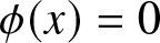 $\phi(x)=0$,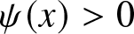 $\psi(x) \gt 0$, with only the third harmonic being present. These waveforms have been found to exist for any $\omega\in(0,2/3)$, which is in line with earlier dynamical observations of the original PDE of Eq. (2.1) [Reference Barashenkov and Alexeeva7]. In the latter the frequency of these waves $3 \omega \lt 2 \Rightarrow \omega \lt 2/3$.Footnote 6 On the other hand, the red line in Figure 1 corresponds to solutions of the $(-,+)$ form, i.e.,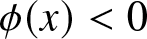 $\phi(x) \lt 0$,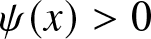 $\psi(x) \gt 0$, in the interval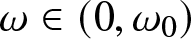 $\omega\in(0,\omega_0)$ with $\omega_0=0.5242$; as one can see, the amplitude of the $\phi$ component tends to zero when $\omega\rightarrow\omega_0$ and becomes zero just at $\omega=\omega_0$. For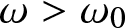 $\omega \gt \omega_0$,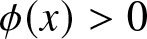 $\phi(x) \gt 0$ and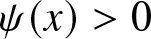 $\psi(x) \gt 0$, meaning that the solution, in our notation, becomes of the $(+,+)$ form, until the solution disappears for only slightly larger frequency, i.e., at $\omega=\omega_+=0.5323$ through a saddle-centre bifurcation with a third branch, also of the $(+,+)$ form and depicted in black. In particular, the branch depicted with a black line has a larger (positive) amplitude within its $\phi$ component, while the red one has a lower amplitude, and the two collide and disappear hand-in-hand at $\omega=\omega_+=0.5323$. However, this saddle-centre event is not the only bifurcation occurring. As the $(-,+)$ branch turns to a $(+,+)$ one with $\phi(0)$ crossing through 0, this red branch ‘collides’ in a transcritical-like bifurcation with symmetry, as we will see below, with the blue branch of the form $(0,+)$. We will explore the implications of these bifurcations for the branches involved in what follows.
(Left panels) Bifurcation diagrams of the solutions to Eq. (2.6) that were identified in our analysis. The values of the first component at  $x=0$ ( $\phi(0)$) and the Hamiltonian defined in Eq. (2.5) are used as a bifurcation diagnostic. The black branch is a $(+,+)$ branch with both components featuring a positive (sign-definite) waveform. The blue solid line represents a $(0,+)$ branch with only the third harmonic being ‘populated’. Finally, the red branch is a $(-,+)$ branch with the two components starting with opposite values, but the first component crosses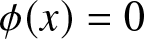 $\phi(x)=0$ when $\omega\rightarrow\omega_0=0.5242$, leading to both components becoming positive before this branch collides in a saddle-centre bifurcation with the other $(+,+)$ branch at $\omega=\omega_+=0.5323$. Dashed lines represent unstable solutions. (Right panels) Profiles of the oscillons for the different branches (from top to bottom: $(+,+)$, $(0,+)$ and $(-,+)$ branches) at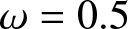 $\omega=0.5$. Green (purple) curves correspond to the $\phi(x)$ ( $\psi(x)$) component.

1 Long description
The image consists of two bifurcation diagrams on the left and three oscillon profiles on the right. The top left diagram plots phi subscript 0 left parenthesis 0 right parenthesis against omega, showing three branches: black, blue and red. The black branch curves upward, the blue branch is horizontal and the red branch curves downward. The bottom left diagram plots H against omega, with dashed lines representing unstable solutions for the same branches. The right side shows three oscillon profiles labeled as black, blue and red branches. Each profile plots phi left parenthesis x right parenthesis and psi left parenthesis x right parenthesis against x, with distinct curves for each branch. The black branch profile shows a higher peak for phi left parenthesis x right parenthesis, the blue branch has a moderate peak and the red branch shows a lower peak for phi left parenthesis x right parenthesis.
In Figure 2, we show the dependence on  $\omega$ of the VK-like quantity discussed earlier, namely, $\omega \int_{\mathbb{R}} \left(\phi^2+9 \psi^2\right) dx$. We observe a maximum of the $(0,+)$ oscillon of the blue branch at $\omega=0.4719$ and another one for the $(-,+)$ oscillon of the red branch at $\omega=0.5200$. Interestingly, for the blue branch, we will see that the change of monotonicity of the relevant quantity is associated with a real eigenvalue changing to imaginary, as the relevant quantity changes from increasing to decreasing. On the other hand, for the black $(+,+)$ branch, the ‘wrong’ monotonicity (i.e., its increasing nature) implies that this branch will always feature real eigenvalue pairs, as we will see to be the case in what follows. Interestingly, the situation for the red branch will be seen in our eigenvalue analysis to be more complicated.
In this figure, we demonstrate the  $\omega \int_{\mathbb{R}} \left(\phi^2+9 \psi^2\right) dx$ quantity that we associated in Theorem 2.4 with stability. The red $(-,+)$ branch changes monotonicity (and hence stability) at $\omega=0.5200$; see also the zoom-in of the right panel. The black $(+,+)$ branch is always increasing and hence always bears real eigenvalues. The blue $(0,+)$ branch has a change of monotonicity at $\omega=0.4719$ analysed further below. Dashed lines represent unstable solutions.

Figure 2 Long description
The left graph shows three curves representing the relationship between omega and the integral of phi squared plus nine psi squared. The x-axis is labeled omega, ranging from 0 to 0.8 and the y-axis is labeled omega times the integral of phi squared plus nine psi squared, ranging from 0 to 4. The blue curve peaks around 0.6, the red curve peaks slightly lower and the black curve is the lowest. The right graph zooms in on the range from 0.51 to 0.53 on the x-axis and from 3.87 to 3.9 on the y-axis. It highlights the red and blue curves, showing a detailed view of their behavior in this specific range. The red curve peaks around 0.52, while the blue curve continues to rise sharply.
Another quantity that was deemed central to our theoretical analysis of Section 4, when constructing the waves, was the functional  $J/I^2$, where $J$ and $I$ are defined in Proposition 4.1. Accordingly, in Figure 3, we illustrate the quantity $J/I^2$ versus $\omega$. One can see that the largest value of the relevant quantity pertains to the black $(+,+)$ branch for $\omega \lt 0.5316$, when the blue branch acquires the largest $J/I^2$ value and becomes the global maximizer until the branch ceases to exist at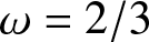 $\omega=2/3$. The relevant global maximizer is unstable throughout its existence (irrespectively of whether it pertains to the black or blue branch), as we will confirm in our eigenvalue analysis.
The quantity  $J/I^2$, where $J$ and $I$ are defined in Proposition 4.1, is given on the left panel for each of the previously discussed branches. The right panel is again a zoom-in where a crossing of this quantity for the black and blue branch takes place at $\omega=0.5316$.

Figure 3 Long description
The left graph shows the relationship between omega (x-axis) and J over I squared (y-axis) with three curves: black, red and blue. The x-axis ranges from 0 to 0.5 and the y-axis ranges from 0 to 0.4. The black curve is the highest, followed by the red and blue curves. The right graph is a zoomed-in view of the left graph, focusing on the range of omega from 0.53162 to 0.53172 and J over I squared from 0.3211 to 0.3215. The black and blue curves intersect within this range, while the red curve remains below them.
We now turn to an analysis of the eigenvalues of the different branches to help elucidate their stability and connect them to the VK-criterion discussed in Theorem 2.4. As discussed already above, and in line with the VK criterion of the Theorem, the  $(+,+)$ branch is always unstable because of a real eigenvalue pair. Figure 4 shows the relevant real part of the (maximal) eigenvalue of the linearization around such solutions. A typical example of the relevant solution and its spectral plane is shown in Figure 5.
Dependence of the real part of the eigenvalues of the  $(+,+)$ family with respect to the frequency. The black line indicates that such a real eigenvalue exists for all the frequencies for which the branch exists, thus rendering it spectrally unstable.

Figure 4 Long description
A graph showing the real part of eigenvalues on the y-axis labeled as 'Re left parenthesis lambda right parenthesis' and frequency on the x-axis labeled as 'omega'. The curve starts at approximately 3.5 on the y-axis and decreases as it moves right, ending near 0.5 on the x-axis and 1 on the y-axis.
Oscillon in the  $(+,+)$ branch with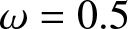 $\omega=0.5$ (left panel) and the corresponding spectral plane featuring a real (unstable) eigenvalue. The green (magenta) curve in the left panel corresponds to the $\phi(x)$ ( $\psi(x)$) component.

Figure 5 Long description
The left graph displays two functions, phi left parenthesis x right parenthesis and psi left parenthesis x right parenthesis, plotted over the x-axis ranging from negative 20 to positive 20. The y-axis ranges from 0 to 0.6. The purple curve represents phi left parenthesis x right parenthesis and the green curve represents psi left parenthesis x right parenthesis. Both curves peak at x equals 0. The right graph shows eigenvalues with the real part on the x-axis ranging from negative 2 to positive 2 and the imaginary part on the y-axis ranging from negative 1 to positive 1. The eigenvalues are represented by circles, with clusters around the real part equals 0 and imaginary parts at approximately positive and negative 0.5.
From the representation of the real and imaginary parts of the spectrum for the  $(0,+)$ solutions in Figure 6, one can observe that such a solution is unstable for $\omega \lt 0.5121$, as at such a value of the frequency parameter, there is a Hopf bifurcation where a quartet of complex eigenvalues becomes imaginary (note that the VK-like quantity does not change monotonicity at this point), while at $\omega=0.4719$, a real eigenvalue pair becomes imaginary as $\omega$ is increased (consistent with the VK-like quantity reaching to a maximum at this point); in addition, at $\omega=\omega_0 \equiv 0.5242$ there is an eigenvalue that becomes zero although it is imaginary past this value. This is fairly remarkable as what happens here is that the positive and negative imaginary parts of the eigenvalue ‘exchange sides’ (i.e., the positive becomes negative and vice versa) without the state changing its stability at the transcritical-like point $\omega_0$. We will use here the term ‘transcritical-like’, since in a regular transcritical bifurcation, the two branches exist both before and after their collision (where they become identical), yet they exchange stability at the critical point. Here, the branches involved collide (meaning that they exist before and after the critical point and coincide at that point), yet due to each of them involving a pair of eigenvalues, their stability is not exchanged; rather, the relevant eigenvalue pairs switch sides (positives become negatives and vice versa, for real eigenvalues in one of the branches and imaginary ones in the other). This behaviour is not predicted by the VK-like quantity.
Dependence of the real (left panel) and imaginary (right panel) parts of the eigenvalues of the  $(0,+)$ family with respect to the frequency $\omega$. A black line indicates that an eigenvalue is real, and red lines are associated with eigenvalues with non-zero imaginary part, i.e., complex ones. Vertical lines correspond to the values of $\omega$ for which the spectral plane is represented in Figure 7. Notice that the solution is fully spectrally stable for $\omega \gt 0.5121$.

Figure 6 Long description
The left graph displays the real parts of eigenvalues plotted against frequency, labeled as omega. The y-axis is labeled Re lambda, ranging from 0 to 1.2. The graph features black and red lines, indicating different eigenvalue behaviors. Vertical dashed lines are present at various frequency values. The right graph illustrates the imaginary parts of eigenvalues, with the y-axis labeled Im lambda, ranging from 0 to 1. Blue lines represent the imaginary components, intersecting and overlapping at different points. Vertical dashed lines are also visible, corresponding to specific frequency values on the x-axis.
Importantly, it is relevant to note that these results are semi-quantitatively in line with the findings of [Reference Barashenkov and Alexeeva7] at the level of the full original PDE of Eq. (2.1), as the latter findings suggest that the single frequency waveform is dynamically robust for  $\sqrt{2}/3 \approx0.4714 \lt \omega \lt 2/3$ in our notation. We indeed identify an eigenvalue transition at $0.4719$ (from real to imaginary) very close to the above threshold, while the complete stabilization of this steady state (when it becomes devoid of Hamiltonian Hopf bifurcations) occurs at $\omega=0.5121$. Some typical examples of the corresponding the $(0,+)$ solution branch spectral planes are shown in Figure 7.
Oscillons in the  $(0,+)$ branch whose frequency corresponds to the dashed vertical lines in Figure 6. Each value of the frequency is displayed at the corresponding panel.

Figure 7 Long description
The image consists of eight spectral plane graphs, each displaying eigenvalues for different omega values. The graphs are arranged in two columns and four rows. Each graph plots imaginary lambda on the y-axis against real lambda on the x-axis, with both axes ranging from negative one to positive one. The omega values are labeled at the top left of each graph: 0.470, 0.480, 0.510, 0.520, 0.523, 0.526, 0.540 and 0.560. The eigenvalues are represented by circles distributed along the vertical axis, indicating their real and imaginary components. The distribution of eigenvalues varies slightly across the different omega values, with some graphs showing more clustered values along the vertical axis than others.
Finally, as can be deduced from Figure 8, the  $(-,+)$ solutions are unstable for $\omega \lt 0.5183$, as at such a value, the oscillon becomes stable via a Hopf bifurcation; i.e., a quartet turns into two imaginary pairs at this frequency. As with the $(0,+)$ case, this bifurcation is not predicted by the VK-like quantity. Importantly, in the case of this branch, the conditions of Theorem 2.1 are not satisfied (as the solutions are not bell-shaped) and hence Theorem 2.4 does not apply. Indeed, this branch with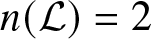 $n({\cal L})=2$ can be observed in Figure 2 (right panel) to have a stable segment even though the VK-quantity is increasing. The relevant branch is stable for a very narrow frequency interval until $\omega=0.5200$, where an eigenvalue pair turns from imaginary to real, leading to the subsequent destabilization of the branch. Notice that we have checked the latter to be consonant with the Hamiltonian–Krein index theory, given that for this branch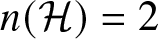 $n({\cal H})=2$, while upon change of monotonicity $n({\cal D})=1$. Hence, per the relevant index theory [Reference Kapitula and Promislow15], there should be $n({\cal H})-n({\cal D})=1$ positive real eigenvalue(s), which is what we observe.
Dependence of the real (left panel) and imaginary (right panel) parts of the eigenvalues of the  $(-,+)$ family on the frequency. The black line indicates a real eigenvalue, while the red lines correspond to eigenvalues with a non-zero imaginary part.

Figure 8 Long description
The left graph shows the real part of eigenvalues, labeled as Re left parenthesis lambda right parenthesis, plotted against frequency, labeled as omega. The x-axis ranges from 0.51 to 0.53 and the y-axis ranges from 0 to 0.8. A black curve starts at approximately 0.52 and rises sharply, while a red curve descends from 0.51 to 0.52. The right graph displays the imaginary part of eigenvalues, labeled as Im left parenthesis lambda right parenthesis, against the same frequency range. The x-axis ranges from 0.51 to 0.53 and the y-axis ranges from 0 to 0.5. Multiple blue curves are visible, with one curve showing a distinct dip around 0.52 before rising again. The graphs illustrate the dependence of eigenvalues on frequency, with distinct real and imaginary components.
As  $\omega$ increases further, again very proximally in frequency, i.e., at $\omega=\omega_0=0.5242$, the collision of the $(-,+)$ and the $(0,+)$ branch discussed above takes place. However, importantly, this is a rather special example of a transcritical-like bifurcation with symmetry. That is to say, as we pointed out above, for the $(-,+)$ branch, the eigenvalues of the real pair exchange sides while both remain real. Accordingly, the $(-,+)$ branch before and after the bifurcation remains unstable, just like the $(0,+)$ branch with which it collides preserves its stability before and after the bifurcation. At the critical point for the $(-,+)$, the $\phi(x)$ component crosses through zero (from negative to positive, as the frequency increases).
Typical examples of relevant solutions in the  $(-,+)$ branch and their spectral planes are shown in Figure 9.
Oscillons in the  $(-,+)$ branch with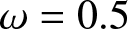 $\omega=0.5$ (top panels), $\omega=0.521$ (middle panels) and $\omega=0.53$ (bottom panels). The left panels show the solution profile, while the right ones show the corresponding spectral plane associated with the branch’s stability. Green (magenta) curves in the left panels correspond to the $\phi(x)$ ( $\psi(x)$) component.

Figure 9 Long description
The image consists of three pairs of graphs. Each pair includes a solution profile on the left and a spectral plane on the right. The left graphs display functions phi(x) and psi(x) plotted over the x-axis, with phi(x) in purple and psi(x) in green. The x-axis ranges from negative 20 to positive 20 and the y-axis ranges from negative 0.2 to positive 0.8. The right graphs illustrate the imaginary part (Im(lambda)) versus the real part (Re(lambda)) of lambda. The x-axis for these graphs varies, with the first graph ranging from negative 1 to positive 1, the second from negative 0.5 to positive 0.5 and the third from negative 0.4 to positive 0.4. The y-axis for all spectral planes ranges from negative 1 to positive 1. Each spectral plane graph contains multiple blue circles representing data points distributed along the vertical axis, indicating the stability of the branch associated with the solution profile. The arrangement of the graphs is in three rows, with each row containing one solution profile and one spectral plane graph side by side.
6.2. Numerical breathers
The oscillons obtained through the solution of Eqs. (2.6) can be used as seeds for fixed point methods that allow to solve the original KG PDE of Eq. (2.1) in the form of periodic orbits (breathers) of the form
 \begin{equation}
z(t,x)=2\sum_{k=1}^\infty y_k(x)\cos\left[(2k-1)\omega_b t\right]
\end{equation}
\begin{equation}
z(t,x)=2\sum_{k=1}^\infty y_k(x)\cos\left[(2k-1)\omega_b t\right]
\end{equation} When this Fourier series expansion is introduced into Eq. (2.1), the PDE is transformed into a system of coupled ODEs, which upon finite difference discretization, turn into a system of algebraic equations. After the choice of a suitable seed and boundary conditions (we have taken periodic ones), it can be solved by means of fixed-point methods like Newton–Raphson (see [Reference Marín and Aubry21] for more details). The numerical domain extends from  $[-L,L]$, where the spatial length parameter here has been chosen as $L=25$.
The main drawback of working with breathers is that they do not exist in a genuinely infinite domain because of resonances of  $k \gt 1$ harmonics with the linear modes band. However, in a finite domain, there can appear gaps in the spectrum that can be controlled by the size of the domain, whose inverse controls the discretization in wavenumbers (and accordingly in frequencies). Then, breathers whose harmonics lie in the resulting frequency gaps have a short interval of stability that is dependent on the domain size and the discretization parameter. In addition, the only oscillon family which gives rise to breathers with features similar to that of the original oscillon is that of the $(0,+)$ solutions above. Because of this, we have only considered breathers coming from the $(0,+)$ branch; in that case, the seed for the fixed point algorithm is taken as $y_1(x)=\psi(x)$ and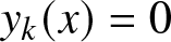 $y_k(x)=0$ for $k\geq2$, and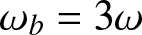 $\omega_b=3\omega$. In this way, one can find breathers that can potentially be stable as we now discuss.
A remark as concerns the  $(-,+)$ and $(+,+)$ modes and their non-existence in the original PDE of Eq. (2.1) is relevant at this point. What we find here is intriguing in that, indeed, there are branches such as $(-,+)$ and $(+,+)$ that may bear complex mathematical structure and associated bifurcations in the reduced model, yet they do not appear – at least, to the best of our ability – in our numerical computations to be featured in the original infinite-dimensional dynamical system. While we maintain that it is of interest [from a mathematical and computational perspective] to explore the stability and bifurcation features of these branches, we believe that it is appropriate to caution physically and computationally minded practitioners about the potential existence of features of the reduced model that ‘may not make it’ to the original PDE model (and vice versa).
6.3. Simulations of the full PDE
Returning to the full model breather solutions, we have considered the dynamics of the KG PDE by taking as an initial condition  $z(0,x)$ a breather with frequency $3\omega$, i.e., $z(0,x)=2\sum_k y_k(x)$ and comparing it with that stemming from an oscillon, i.e., $z(0,x)=2(\phi(x)+\psi(x))$. It is worthwhile to note that in all the relevant examples where the KG PDE is considered, the velocity initial condition $z_t(0,x)$ is set to zero; cf. also Eq. (6.1). Notice that this is also consistent with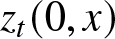 $z_t(0,x)$ as obtained from Eq. (2.3) for real initial condition fields $\phi$ and $\psi$. When considering the $(0,+)$ solution, naturally,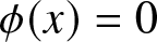 $\phi(x)=0$. Figure 10 considers the dynamics when taking as initial condition an oscillon with $\omega=0.45$ and comparing it with the evolution of a breather with frequency $3\omega$; to this aim, a spatio-temporal diagram is shown together with the spectrum of the Floquet operator of the breather, from which one can see that the dominant instability is of an exponential nature. The evolution of the central site and its Fourier spectrum shown also complements the picture that can be summarized as the emergence of a quasi-periodic breather-like structure that in the case of the initial breather is created after a transient. From the Fourier spectra, one can see that the dominant frequency for the dynamics emerging from the oscillon (breather) is $1.031$ ( $1.717$), and a secondary peak of the spectrum is observed around $0.999$ ( $1.665$). Although the dynamics draws a number of parallels between the two cases, there are also some notable differences. In the approximate oscillon case generated by the steady state solution of Eqs. (2.6), we observe a continuously, yet very slowly decaying structure. On the other hand, the obtained numerically exact solution is indeed a periodic orbit, up to numerical tolerance error, yet this error suffices to eventually destabilize the originally genuinely periodic evolution for sufficiently long times. The resulting structures are similar in nature, albeit with different frequencies involved in the long-term dynamics. Notice also that the frequency peaks at $\omega_p$ in the spectrum of the breather can be associated with the argument $\theta$ of the Floquet exponents related to Hopf bifurcations by $\theta=2\pi(2\omega_p/\omega_b\ \mathrm{mod}\ 1)$. In that case, the dominant peak at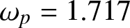 $\omega_p=1.717$ corresponds to $\theta=3.4162$, which is close to the argument of the dominant unstable multiplier $\Lambda=-1.3490 \pm 0.4991\mathrm{i}=1.4384\exp(\pm3.4959\mathrm{i})$.
Spatio-temporal evolution of the energy density for the KG equation using as initial condition a  $(0,+)$ oscillon with frequency $\omega=0.45$ (a) and a (genuinely time-periodic) breather with frequency $3\omega$ (b). Panel (c) shows the time evolution of the central site and also its Fourier spectrum (d) when the oscillon is taken as the initial condition, whereas panels (e) and (f) do the same for the breather; notice that in this case, the Fourier spectrum has been computed from the solution at $x=0$ in the time interval $t\in[400,1000]$. Finally, panel (g) displays the Floquet spectrum of the breather.

Figure 10 Long description
The image contains seven panels labeled (a) to (g). Panel (a) shows a spatio-temporal diagram with axes labeled x and t, depicting energy density evolution with a color scale from 1 to 5. Panel (b) is similar to (a), showing another spatio-temporal diagram with the same axes and color scale. Panel (c) presents a graph of z(t,0) over time t from 0 to 1000, showing oscillatory behavior. Panel (d) displays a Fourier spectrum with axes labeled omega and vertical bar S left parenthesis omega right parenthesis vertical bar, showing a peak around omega equals 1. Panel (e) shows another graph of z(t,0) over time t from 0 to 1000, with a different oscillatory pattern. Panel (f) presents a Fourier spectrum similar to (d), with a peak around omega equals 2. Panel (g) illustrates a Floquet spectrum with axes labeled Re left parenthesis Lambda right parenthesis and Im left parenthesis Lambda right parenthesis, showing points distributed around a circle. Each panel provides insights into the dynamics and spectral characteristics of the system under study.
Figure 11 shows the outcome for the oscillon with 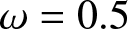 $\omega=0.5$ and the breather counterpart with frequency $3\omega$. In this case, the instabilities of the breather are very weak, and its shape remains almost invariant for the long-time evolutions of the order of 1000 time units reported. It is nevertheless relevant to point out that in this case too, the genuine breather solution is expected to be destabilized for sufficiently long times. Finally, in Figure 12, one can observe that for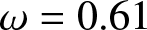 $\omega=0.61$, both the oscillon and the breather are stable, and the oscillon dynamics is quite similar to that of the breather. In addition, we observe the stability of the breather from its Floquet spectrum; in fact, in the bottom right panel of Figure 12, one can see the dependence of the energy versus the breather frequency, and observe the existence of the typical ladders (‘spikes’) caused by the resonance with phonons, i.e., with linear continuous spectrum modes. It is relevant to note here that in the context of oscillons, such a ladder structure has also been reported in the realm of a three-dimensional radial oscillon in a ball in the study of [Reference Alexeeva, Barashenkov, Bogolubskaya and Zemlyanaya3]. Interestingly, for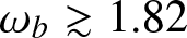 $\omega_b \gt rsim1.82$, the resonances are so small that they cannot be discerned, and the breather is stable for that branch. Prior to the resonance at $\omega_b=1.8199$, the breather solution is stable in the decreasing portion of the branch, while it is unstable in the (narrow) increasing portion evident in Figure 12. While the presence of the continuous spectrum resonances renders the continuation of the relevant breather branch for all frequencies tricky, our expectation is that for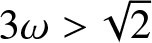 $3 \omega \gt \sqrt{2}$, the breather branch will have a character similar to what is reported above with a typical marginally stable Floquet spectrum (in the exception of small finite-size induced complex [Reference Aubry6] multipliers). Nevertheless, near the resonances with each relevant phonon mode, there will be a portion of increasing energy-frequency dependence, corresponding to breather instability, in line with the corresponding stability criterion of [Reference Kevrekidis, Cuevas-Maraver and Pelinovsky16].
Spatio-temporal evolution of the energy density for the KG equation using as initial condition (a) a  $(0,+)$ oscillon with frequency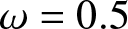 $\omega=0.5$ and (b) a breather with frequency $3\omega$. (c) displays the Floquet spectrum of the breather.

Figure 11 Long description
The image consists of three plots. The first plot (a) shows a heatmap of energy density evolution over time, with the x-axis labeled 'x' ranging from negative 10 to 10 and the y-axis labeled 't' ranging from 0 to 1000. The color scale on the right indicates energy density values from 0.5 to 4.5. The second plot (b) is similar to the first, with the same axes and color scale, showing a slightly different pattern. The third plot (c) is a circular plot of the Floquet spectrum, with the x-axis labeled 'Re left parenthesis Lambda right parenthesis' and the y-axis labeled 'Im left parenthesis Lambda right parenthesis', both ranging from negative 1 to 1. The plot shows a circular distribution of points, indicating the stability of the system being analyzed.
Spatio-temporal evolution of the energy density for the KG equation using as initial condition (a) a  $(0,+)$ oscillon with frequency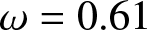 $\omega=0.61$ and (b) a breather with frequency $\omega_b=3\omega=1.83$. (c) displays the Floquet spectrum of the breather and (d) shows the dependence of the energy versus the breather frequency for values of $\omega_b$ near $1.83$.

Figure 12 Long description
The image A shows a graph with x-axis labeled x and y-axis labeled t, depicting energy density evolution with a color scale from 0.2 to 1.6. The image B is similar to A, showing energy density evolution with the same axes and color scale. The image C displays a circular plot with x-axis labeled Re left parenthesis capital lambda right parenthesis and y-axis labeled Im left parenthesis capital lambda right parenthesis, illustrating the Floquet spectrum. The image D shows a graph with x-axis labeled omega subscript b and y-axis labeled H subscript KG, depicting energy versus frequency with a curve showing values from approximately 1.8 to 1.9 on the x-axis and 3 to 4 on the y-axis.
Finally, we have also considered the dynamics of  $(-,+)$ and $(+,+)$ oscillons. As mentioned above, we have been unable to systematically identify breathers pertaining to such steady state solutions; hence, instead, in what follows, we have focused on the initialization of the original KG PDE of Eq. (2.1) with the solution of the steady state problem of Eqs. (2.6). In the case of $(-,+)$ (see Figure 13), we have observed that the oscillon generically disperses, although it still oscillates, as one can see from the panels showing $z(t,0)$; when the frequency increases, the breather dispersion decreases and, potentially, a robust quasi-periodic breather-like excitation is generated. As an example, one can observe that for the $(-,+)$ oscillon with $\omega=0.515$, resulting in a quasi-periodic breather with dominant frequency $1.684$ and secondary frequency $1.370$. For the $(+,+)$ oscillons, the dynamics typically lead to blow up, as one can see in the left panel of Figure 14 (cf. with the right panel of the figure stemming from the $(-,+)$ branch, which leads again to quasi-periodic dynamics).
(Left panels) Spatio-temporal evolution of the energy density for the KG equation using as initial condition a  $(-,+)$ oscillon with frequency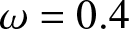 $\omega=0.4$ (panels (a) and (b)), $\omega=0.47$ (panels (c) and (d)), and $\omega=0.515$ (panels (e) and (f)). The right panels show the evolution for $z(t,0)$, i.e., at $x=0$, for the cases in the left panels.

Figure 13 Long description
The image consists of three pairs of graphs. The first pair (a) and (b) shows the spatio-temporal evolution and oscillation pattern for a specific frequency. Graph (a) is a heatmap with x-axis labeled 'x' ranging from -10 to 10 and y-axis labeled 't' ranging from 0 to 40, displaying energy density with a color scale from 0.2 to 1.8. Graph (b) is a line graph with x-axis labeled 't' ranging from 0 to 40 and y-axis labeled 'z(t,0)' ranging from -1 to 1, showing oscillations over time. The second pair (c) and (d) shows similar graphs for another frequency. Graph (c) is a heatmap with x-axis labeled 'x' ranging from -10 to 10 and y-axis labeled 't' ranging from 0 to 40, displaying energy density with a color scale from 0.5 to 2.5. Graph (d) is a line graph with x-axis labeled 't' ranging from 0 to 40 and y-axis labeled 'z(t,0)' ranging from -1 to 1.5, showing oscillations over time. The third pair (e) and (f) shows graphs for a third frequency. Graph (e) is a heatmap with x-axis labeled 'x' ranging from -10 to 10 and y-axis labeled 't' ranging from 0 to 100, displaying energy density with a color scale from 0.5 to 3.5. Graph (f) is a line graph with x-axis labeled 't' ranging from 0 to 100 and y-axis labeled 'z(t,0)' ranging from -1.5 to 1.5, showing oscillations over time.
Spatio-temporal evolution of the energy density for the KG equation using as initial condition a  $(+,+)$ and a $(-,+)$ oscillon with frequency $\omega=0.53$. Left (right) panel corresponds to the case when the initial condition is taken from the black (red) curve of Figure 1.

Figure 14 Long description
The image A shows a heat map with axes labeled x and t, ranging from negative 10 to positive 10 for x and 0 to 3.5 for t. The color scale on the right indicates values from negative 15 to positive 10. The image B shows another heat map with axes labeled x and t, ranging from negative 10 to positive 10 for x and 0 to 100 for t. The color scale on the right indicates values from 0.5 to 4.5.
7. Conclusions and future challenges
In the present work, we have revisited the study of oscillons in one spatial and one temporal dimension in the class of ‘flipped sign’  $\phi^4$ models in the spirit of the work of [Reference Kosevich and Kovalev17]. Motivated by the recent developments in the work of [Reference Alexeeva, Barashenkov, Dika and De Sousa4, Reference Barashenkov and Alexeeva7], we have provided an alternative mathematical approach towards the study of these oscillons, which, however, we have argued extends well past this particular PDE. We have reduced the problem into effectively a two-mode system, concerning the dynamics of the first and third harmonics (given the nature of the cubic nonlinearity). The steady states of the resulting PDE system provide a starting point approximation towards the identification of the full time-periodic oscillon states of the original model. Here we have provided a mathematical analysis, using the tools of index theory, of dynamical systems (through the use of suitable Lyapunov-type functionals) and of nonlinear PDEs, developing quantities whose monotonicity change is tantamount to the change of the steady state’s stability. We have then identified the resulting states numerically and confirmed our stability conclusions, as well as provided a detailed numerical bifurcation analysis of such states, bearing numerous unusual features. These included, e.g., a transcritical-like bifurcation with symmetry but also other bifurcations (such as saddle-centres) between some of the relevant stationary states. Finally, we have compared these findings with the full PDE model, finding good agreement between the existence and stability of one of the branches and the corresponding PDE features. Other of the branches involved significant contributions of higher harmonics and thus led to less meaningful results at the level of full oscillons, although they involved a considerable level of mathematical interest in their reduced model analysis.
We believe that this approach sheds light on a mathematical technique that can be more widely used for periodic solutions in continuum (but possibly also in discrete) problems. Arguably, the resulting reduced PDE models and their steady states are of interest in their own right, yet it seems relevant to establish conditions under which the latter are more closely connected to the original problem and its time-periodic waveforms. In that spirit, such a technique could also be used for the higher-dimensional study and analysis of oscillons, which is of wide relevance to cosmological problems [Reference Gleiser11]. Such studies, both discrete and higher dimensional, of such time-periodic and potentially oscillon-type solutions are currently under consideration and will be reported in future publications.
Data availability statement
The data that support the findings of this study are mostly contained in the paper. Additional datasets can be made available from the corresponding author upon request.
Acknowledgements
We are grateful to Professor Igor Barashenkov for bringing this important problem to our attention, as well as for numerous constructive remarks on this work. This material is based upon work supported by the U.S. National Science Foundation under award, DMS-2210867 (MS), under the awards PHY-2110030, PHY-2408988 and DMS-2204702 (PGK). JC-M acknowledges support from grants PID2022-143120OB-I00 and CEX2024-001517-M, both funded by MICIU/AEI/10.13039/501100011033 and ERDF/EU. This research was partly conducted while PGK was visiting the Okinawa Institute of Science and Technology (OIST) through the Theoretical Sciences Visiting Program (TSVP), the University of Sydney through the visitor program of the Sydney Mathematical Research Institute (SMRI) and the Department of Mechanical Engineering at Seoul National University through a Fulbright Fellowship. Their support is gratefully acknowledged. Finally, this work was also supported by a grant from the Simons Foundation, SFI-MPS-SFM-00011048 (PGK).
Competing interests
The authors declare that they have no competing financial interests or personal relationships that could have influenced the work reported in this paper.
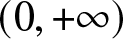



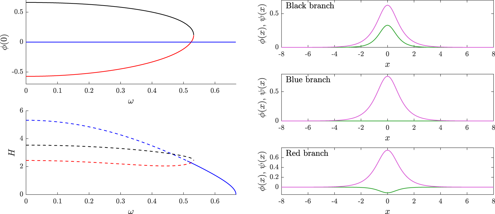


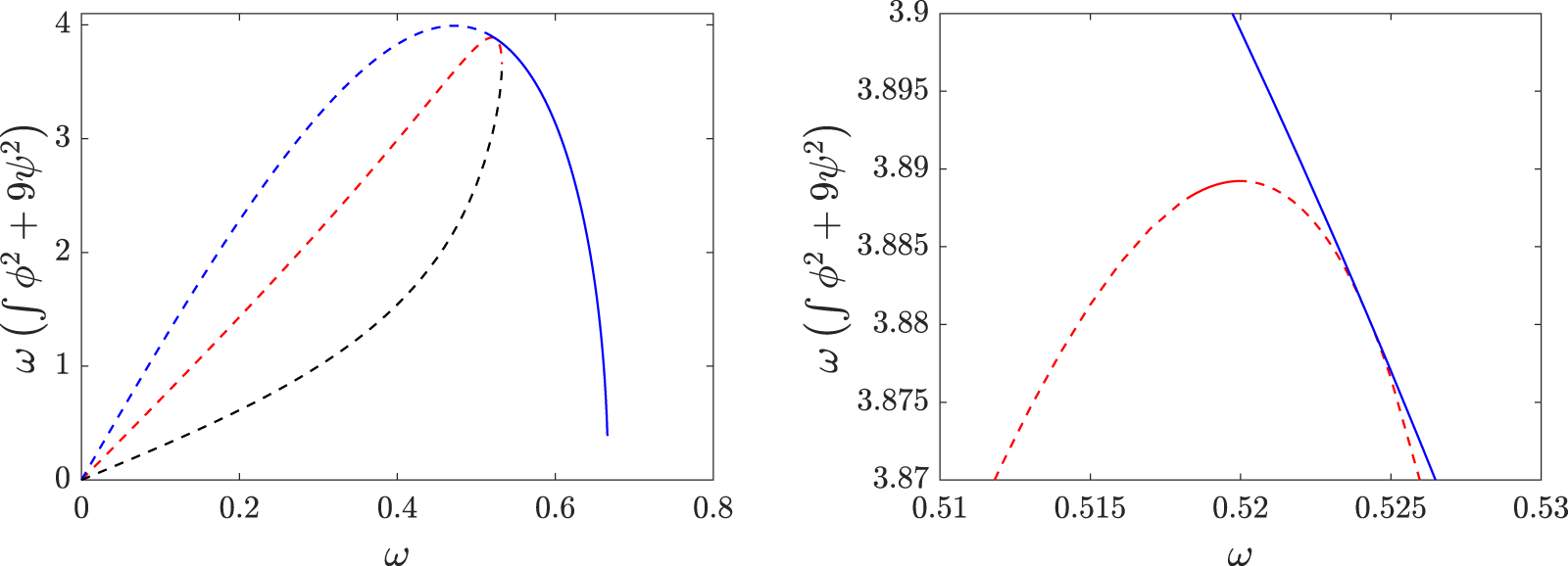


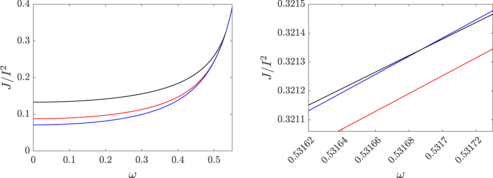


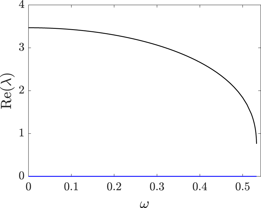

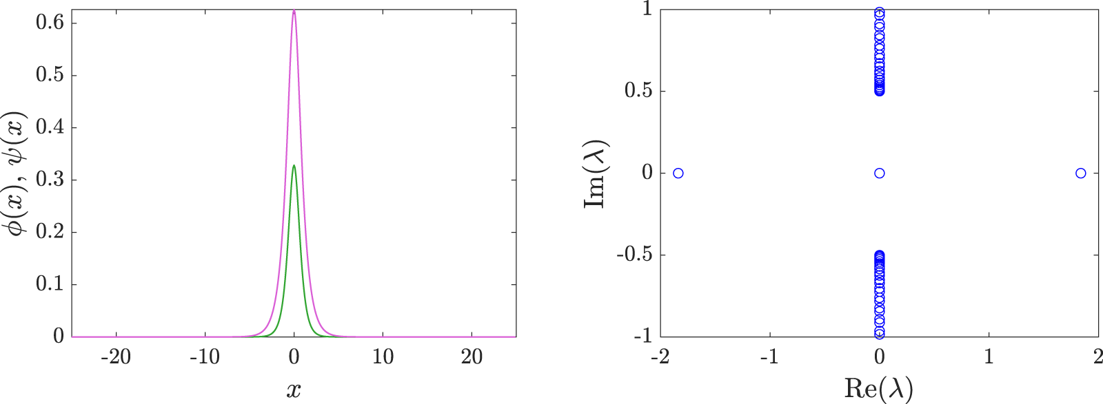


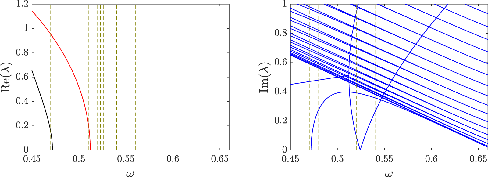


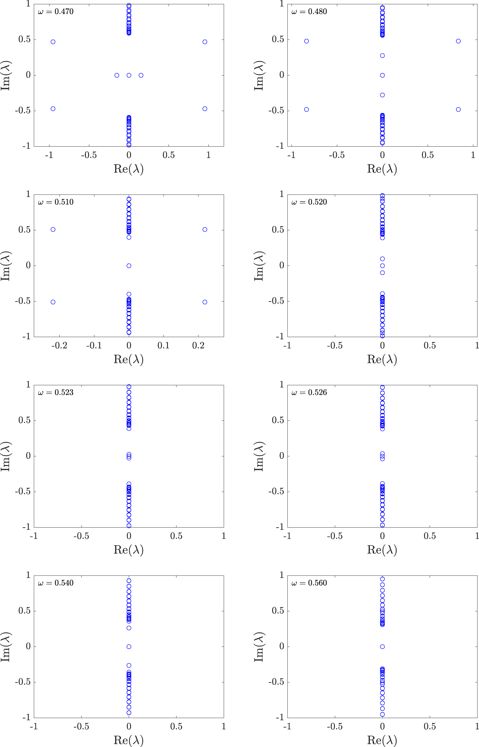

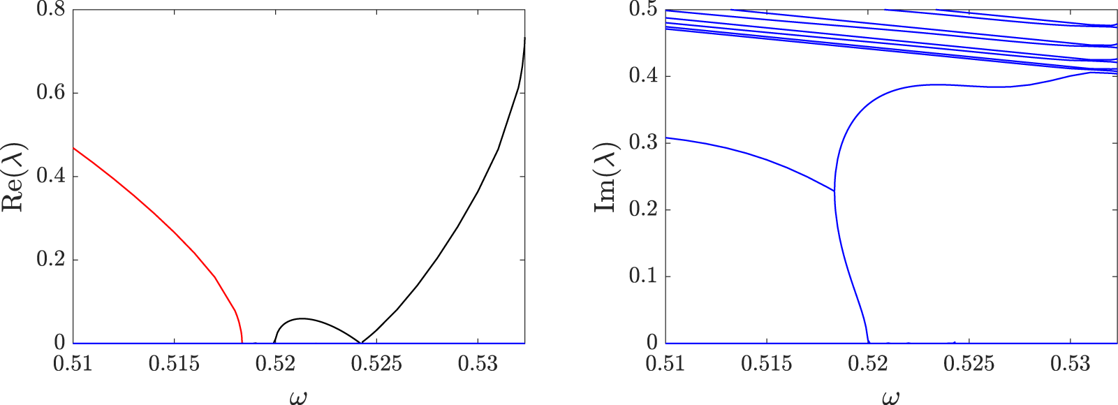

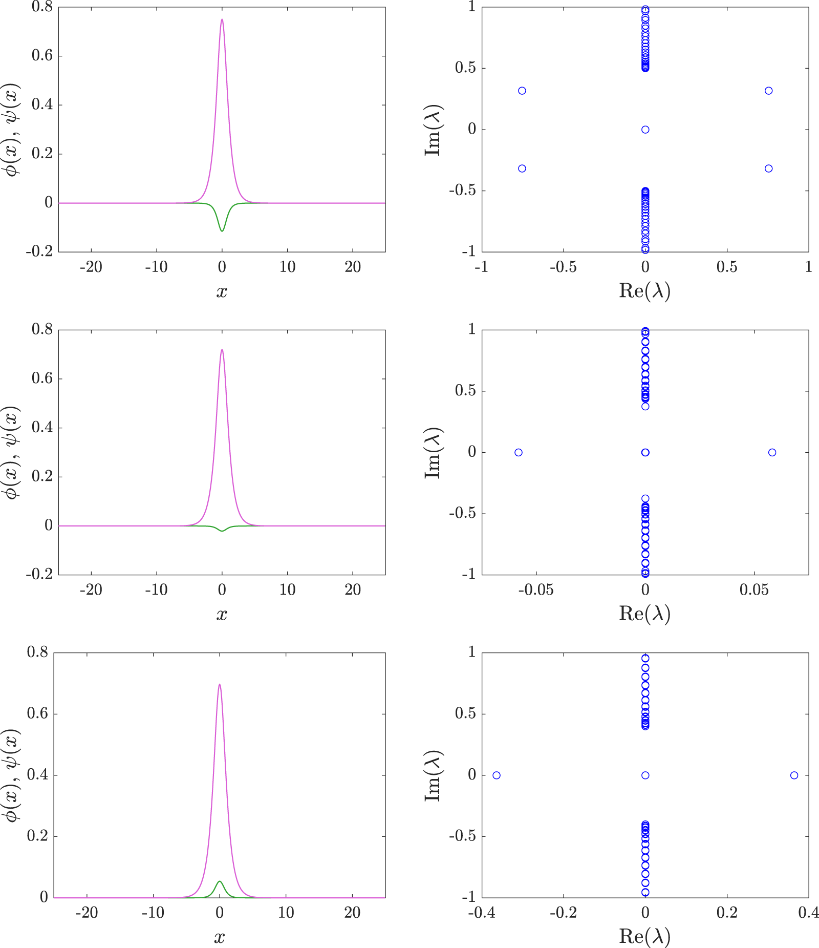


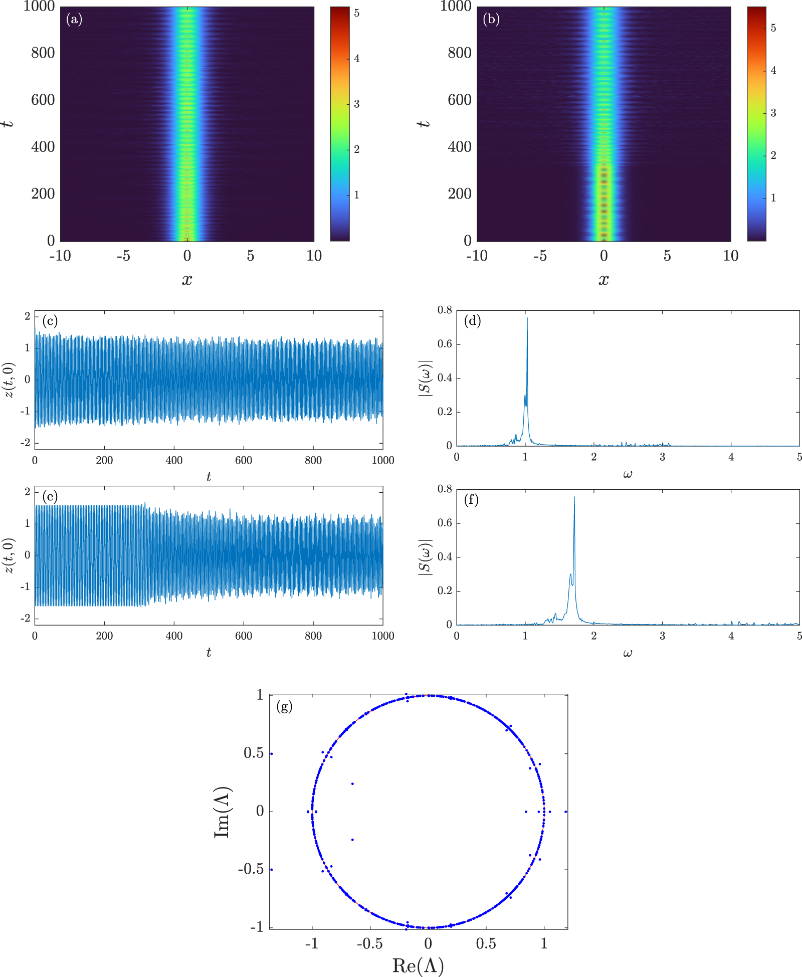


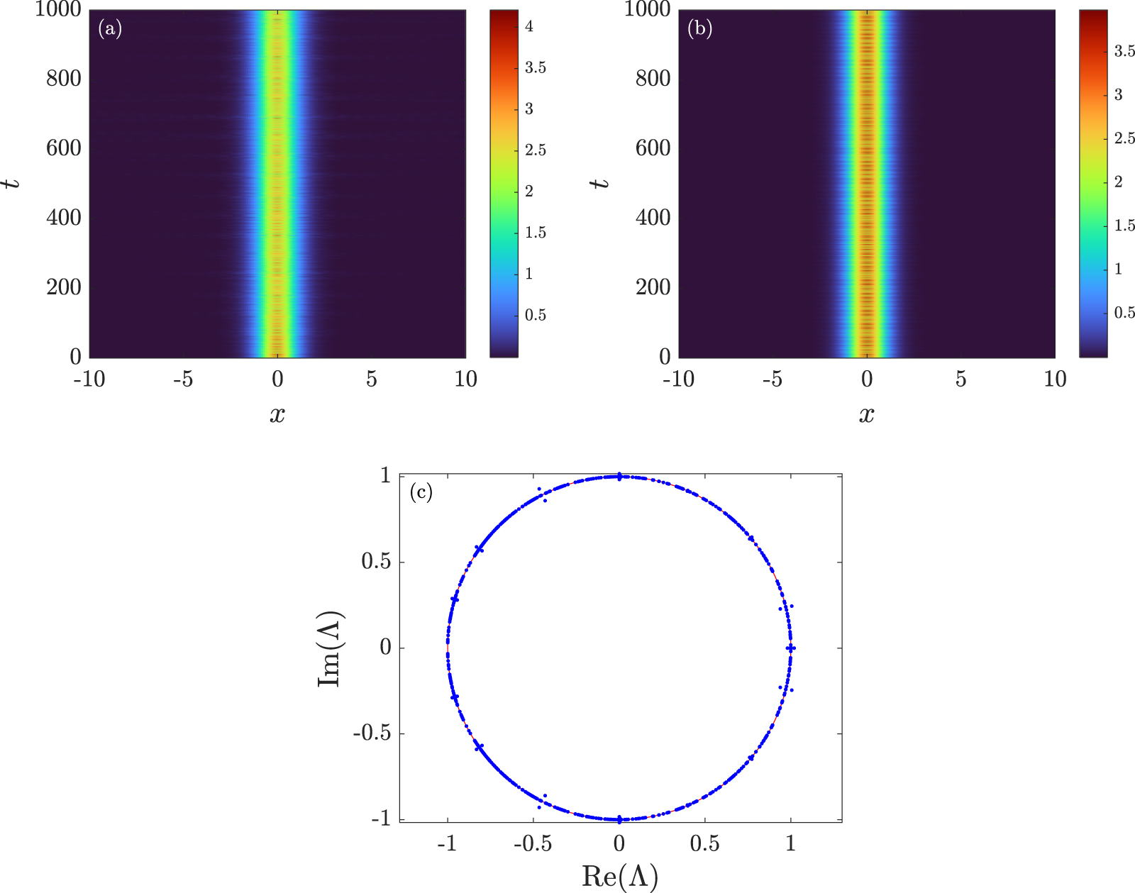


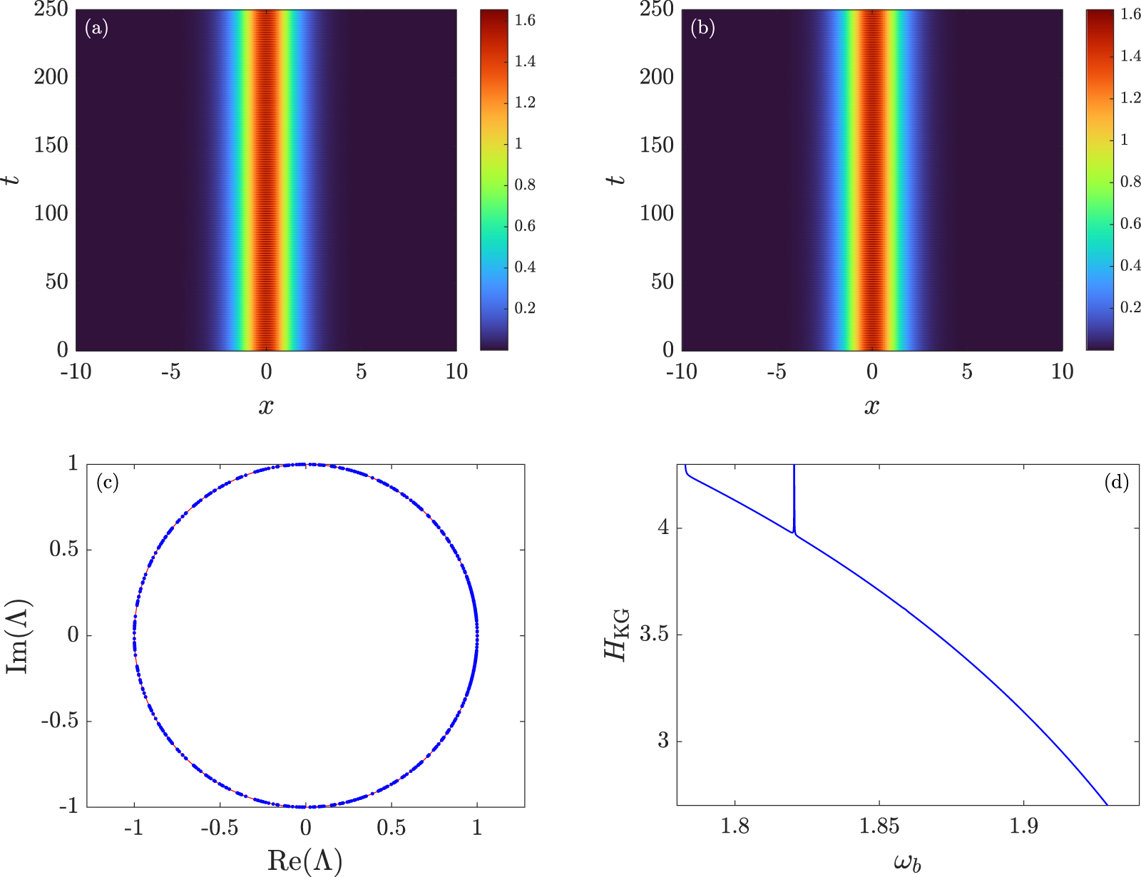


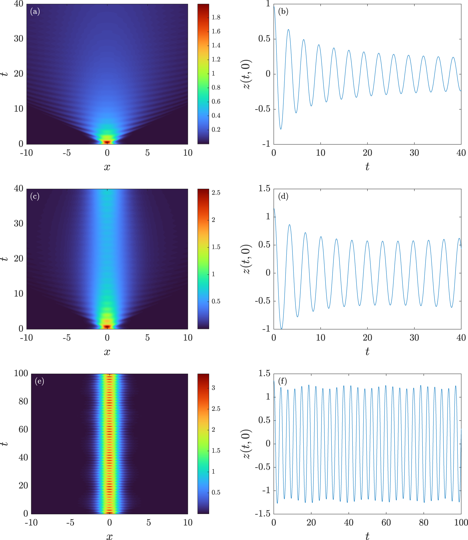


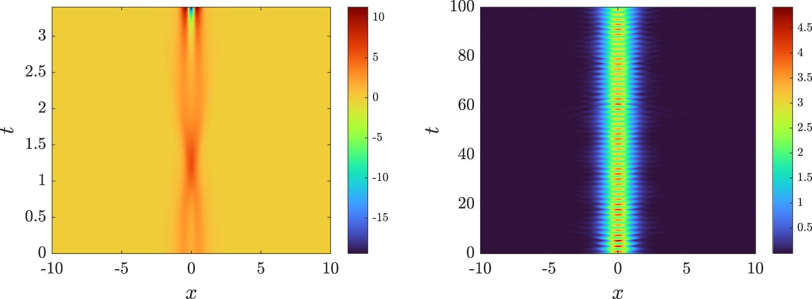


 Open access

