

1. Introduction
Short-term prediction of health expenses is of enormous economic importance for a health insurance company because it has to set the premiums in advance. Underestimation immediately results in underwriting loss, and overestimation in uncompetitive premiums. In the German health insurance market, there are additional legal requirements. In order to prevent adverse selection, the lawgiver has set a financial barrier for the insured to switch to another insurance company. Because this could potentially be exploited by the insurance company, the insurance company has to justify its premium calculation to an independent auditor, called Treuhänder. By law, §2 of KVAV (2017), a loading has to be added to the expected claims to make sure they are certainly sufficient to cover the actual future claims. The independent auditor has to check that the loading is not higher than necessary because that would be to the disadvantage of the insured.
Traditionally, point estimates for the age-dependent expected claims are obtained through simple robust methods, and an additive or relative loading is added by expert judgement. Here, stochastic models can provide a justification for setting this loading: because the premium has to be sufficient on tariff level, one first needs to compute the claim distribution of the tariff as a whole. Then one chooses a risk measure and determines the required capital based on the claim distribution. Finally, one spreads this risk capital in a consistent manner as an additive or relative loading on the age-dependent expected claims.
In practice, the point estimates are obtained through the Rusam method. The basic underlying idea is that all costs in a year increase by the same factor. To be precise, let y t(x) be the average annual cost of a person of age x in the year t. Fix a middle reference age x 0 which has a large number of insured. It is assumed that
 $$y_t (x) \approx y_t (x_0 )k(x),$$
i.e. the costs are estimated as the product of a purely time-dependent factor y t(x 0), which is simply the cost at the reference age, and a purely age-dependent component k(x), called Profil, which is estimated by taking the average across the last couple of years and normalising at the reference age. Forecasts are obtained by linear extrapolation.
Christiansen et al. (Reference Christiansen, Denuit, Lucas and Schmidt2018) fitted several stochastic models to inpatient health claims. Their best fitting model was inspired by the mortality forecasting model of Lee & Carter (Reference Lee and Carter1992), but without the log transformation. It can also be seen as a generalisation of the Rusam method. They assume
 $$y_t (x) = \mu (x) + \kappa (t)\phi (x) + \varepsilon _t (x)\quad {\kern 1pt} with\;{\kern 1pt} \varepsilon _t (x) \sim {\rm{N}}(0,\sigma ^2 )$$
Thus, the average claim is the sum of a purely age-dependent-level term μ(x), an age–time interaction term κ(t)ϕ(x), and an error term. The age–time interaction term is simply the product of a time series κ(t) and a sensitivity per age ϕ(x). The error is assumed to be normally distributed with a standard deviation independent of age and time. The parameters are found by optimisation with respect to the smallest σ. Forecasting is based on the assumption that κ(t) follows a random walk with drift.
Here, we generalise this model by applying the functional data approach:
 $$y_t (x) = \mu (x) + \sum\limits_{j = 1}^J \kappa _j (t)\phi _j (x) + e_t (x) + \varepsilon _t (x)\quad {\kern 1pt} with\;{\kern 1pt} \;e_t (x) \sim {\rm{N}}(0,v^2 (x))\;{\kern 1pt} \;and\;{\kern 1pt} \;\varepsilon _t (x) \sim {\rm{N}}(0,\sigma _t^2 (x))$$
Thus, the age–time interaction term has now more components, and the error distributions now depend heavily on age and loosely on time (for details see section 2). These components give us deeper insight into the changes over time and allow a detailed prediction error estimation. We will also use random walk with drift for the time series κ j(t), but try Holt’s linear models as an alternative, as well. Because the functional data model has so many parameters, they cannot be found by optimisation technics alone – instead the basis functions ϕ j(x) and the coefficients κ j(t) are determined through principal component analysis. This can be easily realised with the R packages ftsa (Hyndman & Shang, Reference Hyndman and Shang2018) and demography (Hyndman, Reference Hyndman2017).
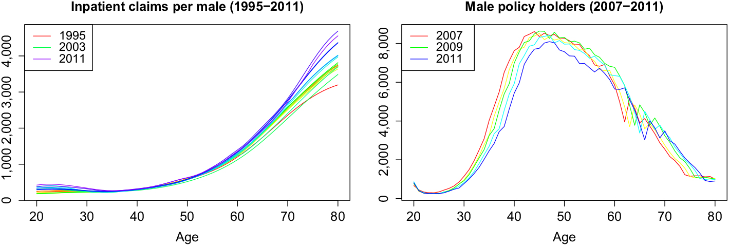
To keep the results here comparable to Christiansen et al. (Reference Christiansen, Denuit, Lucas and Schmidt2018), we use the same data set, the average annual medical inpatient cost per privately insured male of age 20–80 in the years 1996–2011 (see Figure 1 for plots in rainbow colours). These data are provided by the German insurance supervisor BaFin (2018) in order to assist small private insurance companies in their premium calculation and is one of the few publicly available data sets of health expenses per age. The years 1996–2008 will be used for fitting, and the remaining years 2009–2011 for testing. Note the low occupancy at the lower and higher ages. This is likely the cause for the volatility which we will later see at these ages.
Graphical representation of the available data in rainbow colours.
The source code for this study is available at Piontkowski (Reference Piontkowski2018).
2. Functional Data Modelling Approach
The functional data modelling approach for mortality rates was developed by Hyndman & Ullah (Reference Hyndman and Ullah2007) and later refined in Hyndman & Booth (Reference Hyndman and Booth2008) and Hyndman & Shang (Reference Hyndman and Shang2009). Our claims data can be treated similarly to the migration data in Hyndman & Booth (Reference Hyndman and Booth2008).
The main idea is as follows: let y t(x) be the observed average cost per male of age x in year t. It is assumed that it is the realisation of a smooth function f t(x) plus an observational error
 $$y_t (x) = f_t (x) + \varepsilon _t (x)\quad {\kern 1pt} with\;{\kern 1pt} \;\varepsilon _t (x) \sim {\rm{N}}(0,\sigma _t^2 (x)).$$
Note that the smoothing exploits the implicit assumption of a strong correlation between neighbouring ages to improve the quality of the model. The standard deviation σ t(x) is either derived from theoretical considerations like in the mortality case or empirically after the smoothing from the observed ∊ t(x) = y t(x) − f t(x). The latter requires additional assumptions on the time dependence of ∊ t(x), e.g., linearity in t. The time-dependent smooth function f t(x) is decomposed as
 $$f_t (x) = \mu (x) + \sum\limits_{j = 1}^J \kappa _j (t)\phi _j (x) + e_t (x)$$
where μ(x) is the average level, ϕ j (x) a set of orthonormal basis functions, and the coefficients κ j (t) a set of univariate time series. Finally, e t (x) is the approximation error which results from this particular representation. It is assumed to be serially uncorrelated and normally distributed with mean 0 and variance v(x). Thus, the change of f t (x) in time is given by the term Σκ j (t)ϕ j (x). Because the ϕ j (x) are orthonormal, there is no interaction between them and it makes sense to model the time series κ j (t) independently of each other.
This model specialises to the Lee–Carter approach by setting J = 1 and dropping the assumption of a smooth underlying function and thereby merging the errors ∊ t (x) and e t (x) into one.
The modelling process consists of six steps (for details see Hyndman & Ullah (Reference Hyndman and Ullah2007)):
1. Fix a smoothing procedure to obtain f t (x) from the data and estimate the observational standard deviation ∊ t (x). In our case, we are already given the smoothed data, so we can skip this step. Unfortunately, this means that we cannot determine the observational error and have to neglect it.
2. Set the estimator μ̂(x) of μ(x) as the (possibly weighted) mean of the f t (x) across the years.
3. Find ϕ j (x) and κ j (t) through a principal component analysis of ft(x) − μ̂ and choose a appropriately large number J of them for the model. Hyndman & Booth (Reference Hyndman and Booth2008) noted that the forecasts are in general not getting worse with larger J. Compute the residuals e t (x) and estimate v̂(x) from them.
4. Choose a time series model for each of the κ j (t). In general, a random walk with drift is the first choice, but more advanced models have been proven useful and we discuss one option for our data in the following.
5. Forecast as follows: assume the last observed year is t = T. The time series model for the κ j (t) provides us with h-step forecasts k̂ k (T + h), which give us in turn the h-step forecasts
 $$\hat y_{T + h} (x) = \hat f_{T + h} (x) = \hat \mu (x) + \sum\limits_{j = 1}^J \hat \kappa _j (T + h)\phi _j (x)$$
6. Compute the forecast variance with the following explicit formula:
$$Var(\hat y_{T + h} (x)|{\cal I},\{ \mu ,\phi _j \} ) = \hat \sigma _\mu ^2 (x) + \sum\limits_{j = 1}^J u_j (T + h)\phi _j^2 (x) + \hat v(x) + \sigma _t^2 (x)$$
where
$ \mathcal{I} $
stands for the data. σ̂
μ(x) can be derived from the smoothing procedure; e.g. if μ̂x is the mean of y
t
(x) across m years, then
$\hat{\sigma}^2_\mu(x)$
is the sample variance of y
t
(x) divided by m. The coefficient variance u
j
(T + h) = Var(κ
j
(T + h)|κ
j
(T), κ
j
(T − 1), . . . ) follows from the times series model. This formula shows all the different sources of randomness in the model: smoothing method, time series model, approximation error, and observational error.


Hyndman & Shang (Reference Hyndman and Shang2009) showed how to use non-parametric bootstrap methods in order to drop the normality assumptions above.
3. Setting Up the Model
First, we have to decide whether we want to transform the data. The claim curves are rather steep, so a log transformation might be useful. However, the values span only two powers of ten, which is far less than the nine powers of ten in the case of mortality modelling. In addition, after a log transform we optimise the relative error, while we are interested in the absolute error. These are most likely the reasons why the models without a log transformation outperformed the models with one in Christiansen et al. (Reference Christiansen, Denuit, Lucas and Schmidt2018). Thus, we will not apply a log transformation here.
The steps 2 and 3 of the modelling process, i.e. subtracting the mean across time from the data and performing a principal component analysis of the remaining age–time interaction term, can easily be done with function fdm of R package demography. Figure 2 shows the mean ϕ 1, ϕ 2, ϕ 3, ϕ 4 and the first four basis functions ϕ 1, ϕ 2, ϕ 3, ϕ 4 in the top row and the corresponding coefficients κ 1, κ 2, κ 3, κ 4 in the button row. These components explain 90.6%, 7.0%, 1.5%, and 0.4% of the variance. Thus, at least the first two components should be considered in the further modelling process.
Basis functions and associated coefficients of the functional data model.
The first basis function has a shape similar to mean (except at low ages). It represents a general increase of all costs. Roughly, we get the Rusam model if we assume that they have the same shape and the higher components are negligible. The best model of Christiansen et al. (Reference Christiansen, Denuit, Lucas and Schmidt2018), M1, acknowledges that they may be different, but neglects the higher components as well. As the second component explains 7.0% of the variance, we expect a more precise prediction by incorporating it into the modelling process.
The second basis function models shifts of costs at lower and higher ages compared to the middle ages. The third basis function describes the movement of costs at high ages. The fourth basis function models changes in the ages around 30 and 70. However, it explains only 0.4% of the variance and the corresponding coefficient looks like random noise; thus, we will not consider it further.
Looking at the coefficients, we immediately notice the jump in the first coefficient from the year 1995 to 1996 and all coefficients seem to have exceptional behaviour in the years 2003–2004. Outliers in health insurance are most of the time due to changes in the reimbursement system for medical services. In fact, this is here the case. From 1995 to 1996 the cost recovery principle was replaced by a lump compensation system (see Simon (Reference Simon2000)). In 2003 there was a voluntary switch to a new German Diagnosis Related Groups (G–DRG) system. It was made obligatory in 2004, but many hospitals had problems with the switch and were unable to use the system until 2005 (see Böcking et al. (Reference Böcking, Ahrens, Kirch and Milakovic2005) and Ahrens et al. (Reference Ahrens, Böcking and Kirch2004)). Thus, we will drop the data of the year 1995 because of the regime change and the data of the years 2003–2004 because it is certainly flawed.
We refit the model on the remaining data. This time the components explain 93.7%, 5.0%, and 0.8%, thus in total 99.5% of the variance and are plotted in Figure 3. The increase of costs at the younger ages becomes more prominent in the first basis function. The second basis function is mostly devoted to this and is now missing the changes at higher ages. The third basis function is similar to the one before. Again the second and third basis functions together control the behaviour at lower and higher ages. The residuals e t (x) are plotted on the left-hand side of Figure 4. They are slightly less in younger ages, but do not exhibit a trend in time.
Functional data model after outlier removal.

Residuals and interactions in rainbow colours.
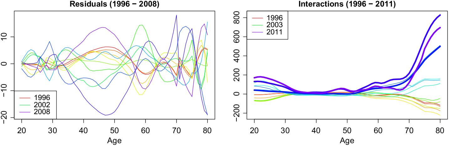
It is very instructive to plot the full age–time interaction, i.e. the data minus the mean across time. We include the years that we want to predict as fat lines (see right-hand side of Figure 4). Again, we note that most changes happen at lower and higher ages. At higher ages, we have a strong increase, which we can read off the first basis function. At the lower ages, there is an increase with some ups and downs, which is the reason for shape of the second basis function besides the first. There have been hardly any changes for the ages from 34 to 53 in the data until 2008, which we use for fitting. But for our test years, we see a bump appearing at the ages 45–55. As these years are between the group from 35 to 44, which is still constant, and the group above 55, which was always volatile, a change in the smoothing method is the most likely explanation. Unfortunately, it is impossible to foresee the appearance of this bump because there was no indication of it before.
4. Time Series Models for the Coefficients κ j
Because we have only few observation years, we should choose a simple and robust time series model, so a random walk with drift (also known as an ARIMA(0,1,0) model with drift) is the natural choice. In this case, the one-step-ahead coefficient κ j(t + 1) arises as the sum of the previous one, a constant drift d j, and a normal distributed error:
 $$\kappa _j (t + 1) = \kappa _j (t) + d_j + \varepsilon _j (t),\quad {\kern 1pt} where\;{\kern 1pt} \varepsilon _j (t) \sim {\rm{N}}(0,\sigma _j^2 )$$
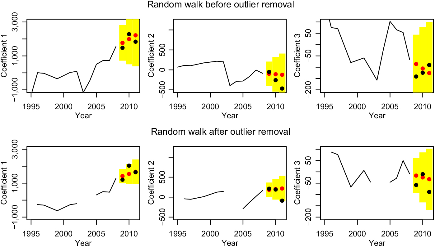
The parameters for the κ j before and after outlier removal are estimated by minimising the square error and shown in Table 1. In both cases, we have an obvious drift in the κ 1, while there is no significant evidence for a drift in κ 2 and κ 3. However, we have no reason to believe that they do not have a drift, so we keep the best estimate. Note that d 1 before outlier removal is much larger than after outlier removal; this is due to the jump of κ 1 from the year 1995 to 1996. Figure 5 shows the predictions in red together with yellow 90% prediction intervals – the true values are given in black. Remember that the basis functions changed a bit through the outlier removal and therefore the coefficients as well. Removing the outliers has roughly halved the prediction intervals. The most dominating coefficient κ 1 is predicted well with the exception of the jump in 2010, which is at the border of the prediction interval in the case with outlier removal. The coefficients κ 2 and κ 3 do in fact look like random noise, but the slight trends improve the predictions and the prediction intervals seem to be plausible. Note in particular that in case with outlier removal, the trend of κ 2 in the years 2005–2008 breaks off immediately in 2009 as the random walk with drift predicts. However, this is not what we would have expected.
Forecasting the coefficients with a random walk with drift before and after outlier removal.
Parameters for the random walk with drift time series

The characteristic of the random walk model with drift is that each jump is fully added to all future values and any two jumps are uncorrelated. Intuitively, we expect that a huge increase of costs to be followed by a smaller one. Thus, we try a second time series model which potentially has the option to capture this, namely the simplest form of exponential smoothing with a linear trend, Holt’s linear trend method (which is equivalent to an ARIMA(0,2,2) model with restrictions on the coefficients). It can be formulated as a state space-model with additive errors as follows (see Holt (Reference Holt2004), Hyndman et al. (Reference Hyndman and Booth2008), and Hyndman & Athanasopoulos (Reference Hyndman and Athanasopoulos2018)):
 $$\matrix{\hfill {} & \hfill {\kappa _j (t + 1)} & \hfill { = l_j (t) + b_j (t) + \varepsilon _j (t),} & \hfill {{\kern 1pt} where\;{\kern 1pt} \varepsilon _j (t) \sim {\rm{N}}(0,\sigma _j^2 )} \cr \hfill {{\kern 1pt} Level:{\kern 1pt} } & \hfill {l_j (t + 1)} & \hfill { = l_j (t) + b_j (t) + \alpha _j \varepsilon _j (t)} & \hfill {{\kern 1pt} for\;{\kern 1pt} 0 \le \alpha _j \le 1} \cr \hfill {{\kern 1pt} Growth:{\kern 1pt} } & \hfill {b_j (t + 1)} & \hfill { = b_j (t) + \beta _j \varepsilon _j (t)} & \hfill {{\kern 1pt} for\;{\kern 1pt} 0 \le \beta _j \le \alpha _j } \cr } $$
The model uses the two latent variables l(t), the trend, and b(t), the growth. In the absence of any randomness l(t) and κ(t) describe a straight line with slope b(t). The parameters α and β determine how much of the observed error is incorporated into the level resp. the slope. Interesting special cases are: (α, β) = (0, 0) is a linear regression; (α, β) = (1, 0) is a random walk with drift b(t) = const.
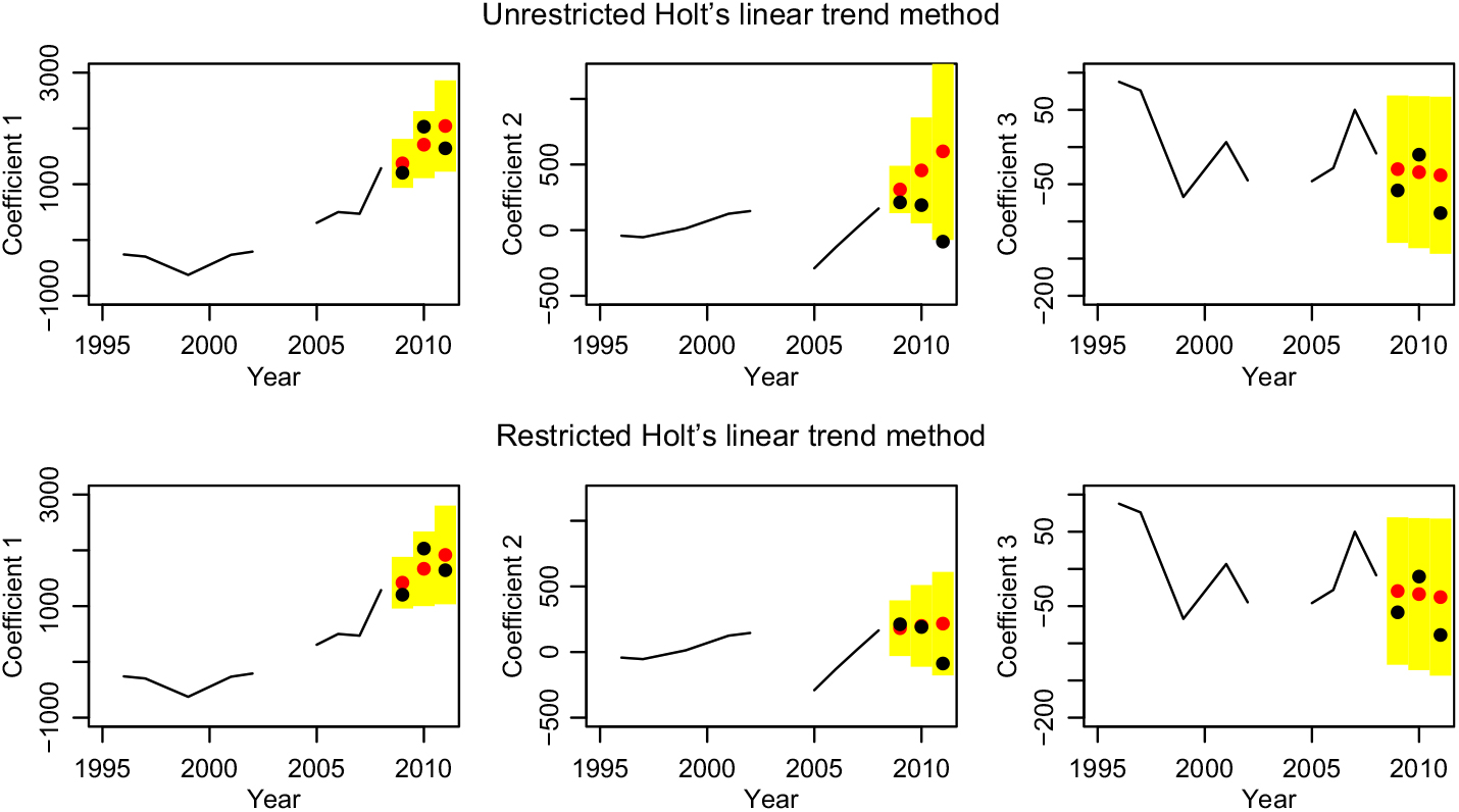
One disadvantage of this model type is that the estimation of the parameters α and β is often unstable (see Auger-Méthé et al. (Reference Auger-Méthé, Field, Albertsen, Derocher, Lewis, Jonsen and Flemming2016)). We estimate again with respect to the minimal mean square error. Unfortunately, the error surface is not guaranteed to be convex, so several local minima may exist (see Chatfield & Yar (Reference Chatfield and Yar1988)). One particular problem is that often the trend gets overestimated (see Gardner & McKenzie (Reference Gardner and McKenzie1985)). This means the growth/slope changes very fast, which is usually undesirable. We use Holt’s linear model only for the functional data model after outlier removal. The parameters are given in the left-hand side of Table 2 and the time series are plotted in top row of Figure 6. We do in fact see large β 1 and β 2, and the high jumps of the second coefficient at the end are extrapolated into the future. While this may look plausible in the figure, remember that it means in reality decreasing health cost at lower ages (even after taking the other components into account), which cannot be true in the long run. We follow the advice of Chatfield & Yar (Reference Chatfield and Yar1988) and restrict β to small values. For the β 1 ≤ 0.23 resp. β 2 ≤ 0.5, the models for κ 1 and κ 2 become the known random walks with drift. So, we require β ≤ 0.25, which is on the one hand the nearly minimal restriction to get a new model and on the other hand still an acceptable rate of change for the trend. Thus, κ 1 has an interesting new model, κ 2 follows a random walk, and κ 3 is modelled by a linear regression; see right-hand side of Table 2 and bottom row of Figure 6.
Forecasting the coefficients with Holt’s linear trend method, unrestricted and restricted.
Parameters for Holt’s linear model
5. Forecasting
In the preceding sections, we defined all the components for three stochastic models – our favourite model is the one after outlier removal with random walk with drift as time series model, as an alternative we use Holt’s linear model with restricted β coefficient as the time series model; finally, we have for comparison the model based on the whole data set with random walk with drift. We are now ready to produce point forecasts as well as prediction intervals.
Figure 7 shows the age–time interaction term for the years 2009–2011; i.e. it corresponds to right-hand side of Figure 4. To get the total claims one has to add the purely age-dependent average level μ(x). It is left out in order to show the time dependence more clearly. Adding it, one gets a graph like the left-hand side of Figure 1, which is dominated by the steepness of μ(x).
Forecasts of the interaction terms for the years 2009–2011 (black = actual, fat red = prediction, thin red = 90% prediction intervals based on the variance formula, yellow shaded areas = 90% prediction intervals based on non-parametric bootstrap methods, grey = best approximation given the chosen basis functions).
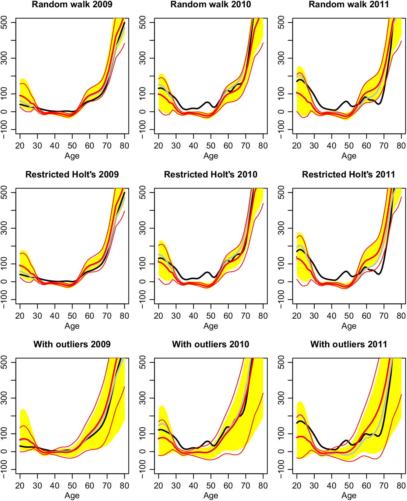
The black lines are the actual interaction terms. The fat red lines are the predicted ones. The grey lines show the best approximation possible to the actual data with the chosen basis functions. The thin red lines are the 90% prediction intervals based on the variance formula of section 2 and normality assumption. Finally, the yellow shaded areas are the prediction intervals based on Monte Carlo simulation, where the unknown error distributions are simulated by the bootstrap method of Hyndman & Shang (Reference Hyndman and Shang2009). The latter is implemented in the simulate function of the R package demography.
A gap between the black and the grey curves tells us that the claim curve has a new shape feature that has not been important before. This is here the case for the middle ages. We expected this already while looking at the interaction terms in Figure 4. There we saw an increase of the claim amounts for these ages, which have been nearly constant in all the years before. A gap between the grey and the red curves indicates errors in the time series prediction. Here, we note in particular that we underestimate the development at the young ages in 2011. This corresponds to the sharp drop of coefficient 2 in Figures 5 resp. 6. The behaviour of coefficient 2 is rather erratic and therefore hard to predict. The reason for this is most likely the low exposure in this age group, see Figure 1, which in turn means that this age group is economically less important. Another widening gap appears at the ages between 55 and 70. However, this error switches signs between 2010 and 2011; thus, it does not have to be systematic. Also, the prediction intervals are rather large in this age group, so precise predictions are difficult here. In fact, for this age group, the predictions of the models differ the most. Forecasting with Holt’s linear method is better compared to random walk with drift in 2010, but worse in 2011.
Turning to the prediction intervals, we immediately notice the huge intervals if we do not remove the outliers. But even these cannot capture the beforehand unseen change in the middle ages. With the removal of the outliers, the prediction intervals become very narrow. The grey curves stay inside; this follows essentially from the fact that time series predictions stay inside their prediction intervals in Figures 5 resp. 6, but the actual claim curve in black moves outside these bound while it evolves into beforehand unseen shapes. The computationally less expensive approximation of the prediction intervals by the variance formula and normality assumption is most of the time good, and exceptions occur when the intervals are very wide – at the younger ages and for the lower bounds in the case without outlier removal.
Standard quality measures in form of the rooted mean square error (RMSE) and the mean absolute error (MAE) are given in Table 3. For comparison, the best model of Christiansen et al. (Reference Christiansen, Denuit, Lucas and Schmidt2018), M1, is included. Note that for the model M1 outlier removal was not performed. As we have already seen in Figure 7, the model with Holt’s linear trend method is better in 2010, but worse in 2011 than the model with the random walk with drift. Both give slightly better predictions than the M1 model. However, the main improvement of the models here compared to M1 is the more refined error structure. Firstly, we use here an age-dependent approximation and observation error with variance v(x) resp. $\sigma^2_t(x)$
. Secondly, we use more components for the age–time interaction and take the uncertainties of the time series prediction for the coefficients κ
j
(t) into account, which were neglected in the M1 model. Together this leads to more age-specific prediction intervals.
$\sigma^2_t(x)$
. Secondly, we use more components for the age–time interaction and take the uncertainties of the time series prediction for the coefficients κ
j
(t) into account, which were neglected in the M1 model. Together this leads to more age-specific prediction intervals.
RMSE and the MAE for the models

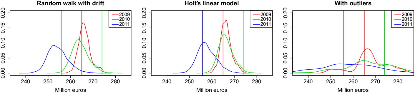
As an application of the stochastic model, we predict the distribution of the total claim expenses of all insured in the years 2009–2011 (see Figure 8). Again, we see how strongly the removal of the outliers influences the uncertainty of the predictions. In 2009 and 2011, the actual expenses are close to the maximum of the distribution, while for 2010, the total expenses are underestimated due to the previously unseen increase of expenses in the middle ages. In 2011, this is compensated by a reduction of expenses in the age group from 60 to 70.
Forecasted total expenses.
6. Conclusion and Outlook
The functional data approach gave us deeper insight into the data. The first three basis functions had obvious meanings: an overall increase of expenses and special trends at the younger resp. older ages. The jumps in the coefficients led us to suspect outliers, which were in fact caused by legal changes. For forecasting the coefficient time series the canonical choice was random walk with drift, which worked well. As an alternative we discussed the use of Holt’s linear model. It is more flexible, and the drift can adapt over time. However, it is difficult to fit because parameter estimates become more uncertain. The reason is that Holt’s model is equivalent to an ARIMA(0,2,2) model, i.e., second-order differences have to be computed. As our data cover only a few years and contain lots of noise, those get unstable and lead to uncertain parameters. Thus, Holt’s linear model should be used with caution. From the functional data model, we obtained detailed prediction error estimates, which helped us to analyse the test cases.
For this particular claim data set, the analysis revealed again the main obstacles for a precise prediction of health expenses. Firstly, legal and administrative changes introduce outliers or even regime changes, which make the data before them less informative. Secondly, changes in the data collection or smoothing method over time cause further inconsistencies.
This suggests a direction for future research: develop the functional data approach further to allow a weighted influence of the years on the model, outlier years or years before a regime change should have less influence than the more recent years. The ideas of Hyndman & Shang (Reference Hyndman and Shang2009) will be a good starting point.
Further, the methods here should be applied to the individual tariffs of an insurance company. There one has the raw data and can choose the smoothing method oneself. However, because inpatient claims are very volatile and the number of insured is only in the tens of thousands, one faces a large observational error. Hence, credibility methods should be developed; i.e. the data of all available tariffs should be used to make the prediction for each individual tariff more robust.


 Open access