





Impact statement
We present a dynamical autoencoder (DnAE) framework that couples cAEs with neural ordinary differential equations (ODEs) to predict ignition trajectories in laser-ignited rocket combustors. The problem representation first reduces the simulation data from high-dimensional fields of primitive variables to path-integrated quantities that mimic experimental data acquisition. The resulting quantities are compressed via cAEs to a low-dimensional manifold, and subsequently, temporal evolution is forecast with parameterized neural ODEs, extending the application of such models beyond existing simple dynamics emulators to a complex engineering problem of interest. The DnAE reduces ignition prediction cost by orders of magnitude relative to large-eddy simulation while accurately capturing bifurcating ignition success and failure dynamics, representing a step toward real-time digital twins for propulsion systems.
1. Introduction
Surrogate models are commonly used to accelerate the search for promising designs by replacing expensive evaluations or simulations (Forrester et al., Reference Forrester, Sobester and Keane2008) or to estimate variability in quantities of interest (QoI) for an engineering system (Sudret et al., Reference Sudret, Marelli and Wiart2017). In many engineering applications, the surrogate represents a mapping
$ f:{\unicode{x211D}}^d\to \unicode{x211D} $
 , where the input vector
$ \boldsymbol{\xi} =\left({\xi}_1,\dots, {\xi}_d\right) $
, where the input vector
$ \boldsymbol{\xi} =\left({\xi}_1,\dots, {\xi}_d\right) $
 encodes design parameters and variables describing the uncertainty present in the system, and the output is a scalar representing local or system-level performance measures. There is no shortage of applications; examples include polynomial chaos expansions applied to wake flows (Lee et al., Reference Lee, Chan, Zahtila, Lu, Iaccarino and Ooi2025; Lu et al., Reference Lu, Zahtila, Chan, Nguyen, Lei, Iaccarino and Ooi2025) and Gaussian process regression used to compare experiments and simulations of a prism bluff body (Duan et al., Reference Duan, Cooling, Ahn, Jackson, Flint, Eaton and Bluck2019). Prediction of field quantities is more challenging and does not always provide direct engineering insight. Nonetheless, vector-to-vector surrogates of the form
$ f:{\unicode{x211D}}^d\to {\unicode{x211D}}^m $
encodes design parameters and variables describing the uncertainty present in the system, and the output is a scalar representing local or system-level performance measures. There is no shortage of applications; examples include polynomial chaos expansions applied to wake flows (Lee et al., Reference Lee, Chan, Zahtila, Lu, Iaccarino and Ooi2025; Lu et al., Reference Lu, Zahtila, Chan, Nguyen, Lei, Iaccarino and Ooi2025) and Gaussian process regression used to compare experiments and simulations of a prism bluff body (Duan et al., Reference Duan, Cooling, Ahn, Jackson, Flint, Eaton and Bluck2019). Prediction of field quantities is more challenging and does not always provide direct engineering insight. Nonetheless, vector-to-vector surrogates of the form
$ f:{\unicode{x211D}}^d\to {\unicode{x211D}}^m $
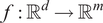 have been explored, where the input encodes parametric dependence or initial conditions, and the output is a reduced feature-space representation of the flow field. Examples include parametric extensions of proper orthogonal decomposition (POD) for compressible aerodynamics (Bui-Thanh et al., Reference Bui-Thanh, Damodaran and Willcox2003), and temporal extensions of POD such as dynamic mode decomposition (DMD) applied in a predictive capacity to simple partial differential equations (PDEs) (Lu and Tartakovsky, Reference Lu and Tartakovsky2020). More recently, for steady aerodynamic fields, nonlinear dimensionality reduction has proven to be capable of extreme compression (Saetta et al., Reference Saetta, Tognaccini and Iaccarino2024b), and the flexibility of neural network architectures has facilitated strategies for entire flow-field generation. Subsequent extensions that encompass time-series learning efforts have notably used long short-term memory networks, transformers (Solera-Rico et al., Reference Solera-Rico, Vila, Gómez-López, Wang, Almashjary, Dawson and Vinuesa2024), and neural ordinary differential equations (neural ordinary differential equations [ODEs]/NODEs) to learn latent spaces of simpler spectrum problems such as the 1D Kuramoto–Sivashinsky equation for evolution on an inertial manifold (Linot and Graham, Reference Linot and Graham2022), or two-dimensional Kolmogorov flow (Chakraborty et al., Reference Chakraborty, Chung, Arcomano and Maulik2024). Neural ODEs provide a simpler, dynamics-consistent framework whose behavior is easy to inspect, in contrast to the comparatively complicated transformer architectures, which are more akin to a black-box model.
In the present study, a surrogate framework is applied to a reliability study in the context of rocket ignition success. In particular, we wish to assess binary ignition sensitivities in the combustor, in response to a high-dimensional input parameter space. A secondary aim is that the surrogate model provides realistic time-resolved spatial dynamics, which rules out the use of standard supervised classification methods. A natural approach to surrogate modeling is to first build a database, consisting of precalculated samples obtained from classical simulation methods, which then trains the surrogate model across an input parameter vector
$ \boldsymbol{\xi} $
 , with components
$ {\xi}_i $
, with components
$ {\xi}_i $
 sampled according to their input probability distributions, e.g.,
$ \Pr \left({\xi}_i\right)\sim \mathcal{N}\left(\mu, {\sigma}^2\right) $
sampled according to their input probability distributions, e.g.,
$ \Pr \left({\xi}_i\right)\sim \mathcal{N}\left(\mu, {\sigma}^2\right) $
 or
$ \Pr \left({\xi}_i\right)\sim \mathcal{U}\left(a,b\right) $
or
$ \Pr \left({\xi}_i\right)\sim \mathcal{U}\left(a,b\right) $
 , and in this study chosen to be experimentally informed where possible (Strelau et al., Reference Strelau, Frederick, Winter, Senior, Gejji and Slabaugh2024). In a laser-ignited rocket combustor context, each time a laser deposits an energy kernel, significant variability in the laser operating conditions (Zahtila et al., Reference Zahtila, Passiatore and Iaccarino2023) and more generally in the combustor system occurs, meaning that (i) no two ignition trials are the same, and (ii) variations in the system input space
$ \boldsymbol{\xi} $
, and in this study chosen to be experimentally informed where possible (Strelau et al., Reference Strelau, Frederick, Winter, Senior, Gejji and Slabaugh2024). In a laser-ignited rocket combustor context, each time a laser deposits an energy kernel, significant variability in the laser operating conditions (Zahtila et al., Reference Zahtila, Passiatore and Iaccarino2023) and more generally in the combustor system occurs, meaning that (i) no two ignition trials are the same, and (ii) variations in the system input space
$ \boldsymbol{\xi} $
 can lead to bifurcating outcomes in the system response. Whether a deposited laser kernel will lead to a kernel evolution sequence with a successful ignition future state depends on the spatiotemporal evolution of the system, motivating a vector-to-vector surrogate. To predict whether ignition will occur, scale-resolving large-eddy simulation (LES) provides a physically accurate and computationally tractable approach among classical simulation strategies, such as Reynolds-averaged Navier–Stokes, and direct numerical simulation (DNS), with predictive ability for the current problem validated against experiments (Brouzet et al., Reference Brouzet, Zahtila, Rossinelli, Voci, Iaccarino, Passiatore, Strelau, Gejji and Slabaugh2025). An LES computation of an ignition trial amounts to time integration of high-dimensional 3D spatial field and is therefore still a costly calculation for the purpose of a single realization of ignition success. In this work, we first carry out an ensemble of LES calculations as ignition trials (Zahtila et al., Reference Zahtila, Cutforth, Brouzet, Passiatore, Rossinelli and Iaccarino2025) to characterize the output space, capturing both input system variability and the resulting multimodal outcomes.
Building on this ensemble of LES trials, a data matrix of spatiotemporal flow realizations is constructed as
$ \mathcal{S}={\cup}_{j=1}^{N_c}\left\{{\mathbf{x}}^{(j)}\left({t}_0\right),{\mathbf{x}}^{(j)}\left({t}_1\right),\dots, {\mathbf{x}}^{(j)}\left({t}_{N_t-1}\right)\right\} $
 , where
$ {\mathbf{x}}^{(j)}\left({t}_i\right)\in {\unicode{x211D}}^d $
, where
$ {\mathbf{x}}^{(j)}\left({t}_i\right)\in {\unicode{x211D}}^d $
 , with
$ d $
, with
$ d $
 the dimension of the flattened data snapshot,
$ i=0,\dots, {N}_t-1 $
the dimension of the flattened data snapshot,
$ i=0,\dots, {N}_t-1 $
 the discrete snapshot index, and
$ j=1,\dots, {N}_c $
the discrete snapshot index, and
$ j=1,\dots, {N}_c $
 the LES case index, each with a new input parameter sample
$ {\boldsymbol{\xi}}^{(j)} $
the LES case index, each with a new input parameter sample
$ {\boldsymbol{\xi}}^{(j)} $
 . Each individual data snapshot
$ {\mathbf{x}}^{(j)}\left({t}_i\right) $
. Each individual data snapshot
$ {\mathbf{x}}^{(j)}\left({t}_i\right) $
 comes from a 2D integrated representation of the 3D flow field (detailed later in the manuscript). The constructed LES dataset therefore captures the range of spatiotemporal dynamics induced by the sampled ensemble of input uncertainty vectors
$ \boldsymbol{\xi} $
comes from a 2D integrated representation of the 3D flow field (detailed later in the manuscript). The constructed LES dataset therefore captures the range of spatiotemporal dynamics induced by the sampled ensemble of input uncertainty vectors
$ \boldsymbol{\xi} $
 and forms the starting point for reduced-order modeling. The choice and construction of 2D representation for the flow field is crucial because the present system represents an instance of the compressible reacting Navier–Stokes equations and therefore contains many flow features such as shock–shear layer interactions, vorticity in the shear layer with associated turbulence spectrum, and hydrodynamic ejection caused by laser-induced optical breakdown (Wang et al., Reference Wang, Buchta and Freund2020). The main idea is that the three-dimensional flow field can first be reduced to an informative two-dimensional representation, such as through integrated fields, that retains the physics relevant to ignition while omitting information that is not central to the prediction task. These representations can then be compressed into a low-dimensional latent space, whose coordinates are learnable as functions of the input parameter vector. The present framework therefore nonlinearly spatially compresses the dataset through autoencoders (AEs) and subsequently learns trajectories in the latent space through a neural ODE. These two components together are sufficient to build a spatiotemporal surrogate model.
1.1. Dimensionality reduction
Dimensionality reduction is a well-established technique in fluid mechanics and has been popular for extraction of flow features and flow modes (Brunton et al., Reference Brunton, Noack and Koumoutsakos2020; Jaroslawski et al., Reference Jaroslawski, Patil and McKeon2025; Lu et al., Reference Lu, Chan and Ooi2025). The most popular technique is POD, in which a field is expanded as
$ u\left(\mathbf{s},t\right)={\sum}_{k=1}^{\infty }{a}_k(t){\phi}_k\left(\mathbf{s}\right) $
 , where
$ \mathbf{s} $
, where
$ \mathbf{s} $
 denotes spatial position,
$ {\phi}_k\left(\mathbf{s}\right) $
denotes spatial position,
$ {\phi}_k\left(\mathbf{s}\right) $
 are orthonormal spatial basis functions, or POD modes, that capture the dominant structures in the data, and
$ {a}_k(t) $
are orthonormal spatial basis functions, or POD modes, that capture the dominant structures in the data, and
$ {a}_k(t) $
 are the corresponding time-dependent modal coefficients. POD projects the dataset
$ \mathcal{S} $
are the corresponding time-dependent modal coefficients. POD projects the dataset
$ \mathcal{S} $
 onto an optimal linear basis, and this may be useful firstly in inspecting the POD modes to determine the flow structures ranked in terms of energy content, but second, a truncated representation can serve as a reduced basis for compression of the original dataset. Although POD is successfully able to identify dominant coherent structures, it often requires a large number of modes to capture multiscale turbulence (Alfonsi and Primavera, Reference Alfonsi and Primavera2007; Muralidhar et al., Reference Muralidhar, Podvin, Mathelin and Fraigneau2019) and can become unreliable when strong nonlinear dynamics dominate, motivating alternatives such as DMD (Schmid, Reference Schmid2022). A machine learning counterpart to POD is the AE, which encodes the data matrix into a compact latent space and subsequently decodes it for reconstruction. For a shallow two-layer AE with linear activation functions, the learned basis recovers the POD modes (Milano and Koumoutsakos, Reference Milano and Koumoutsakos2002), so that choosing a latent dimension
$ {N}_{\mathrm{\ell}} $
onto an optimal linear basis, and this may be useful firstly in inspecting the POD modes to determine the flow structures ranked in terms of energy content, but second, a truncated representation can serve as a reduced basis for compression of the original dataset. Although POD is successfully able to identify dominant coherent structures, it often requires a large number of modes to capture multiscale turbulence (Alfonsi and Primavera, Reference Alfonsi and Primavera2007; Muralidhar et al., Reference Muralidhar, Podvin, Mathelin and Fraigneau2019) and can become unreliable when strong nonlinear dynamics dominate, motivating alternatives such as DMD (Schmid, Reference Schmid2022). A machine learning counterpart to POD is the AE, which encodes the data matrix into a compact latent space and subsequently decodes it for reconstruction. For a shallow two-layer AE with linear activation functions, the learned basis recovers the POD modes (Milano and Koumoutsakos, Reference Milano and Koumoutsakos2002), so that choosing a latent dimension
$ {N}_{\mathrm{\ell}} $
 corresponds to retaining the first
$ {N}_{\mathrm{\ell}} $
corresponds to retaining the first
$ {N}_{\mathrm{\ell}} $
 POD modes. The latent representation is given by the vector
$ \mathbf{V}=\left({V}_0,\dots, {V}_{N_{\mathrm{\ell}}-1}\right)\in {\unicode{x211D}}^{N_{\mathrm{\ell}}} $
POD modes. The latent representation is given by the vector
$ \mathbf{V}=\left({V}_0,\dots, {V}_{N_{\mathrm{\ell}}-1}\right)\in {\unicode{x211D}}^{N_{\mathrm{\ell}}} $
 , where each component
$ {V}_{\mathrm{\ell}} $
, where each component
$ {V}_{\mathrm{\ell}} $
 is a latent coordinate learned from the data. When nonlinear activation functions are introduced, the network instead learns a nonlinear manifold embedded in the full state space
$ \mathcal{M}\subset {\unicode{x211D}}^d $
is a latent coordinate learned from the data. When nonlinear activation functions are introduced, the network instead learns a nonlinear manifold embedded in the full state space
$ \mathcal{M}\subset {\unicode{x211D}}^d $
 , allowing more aggressive compression than linear POD (Zeng et al., Reference Zeng, Linot and Graham2022; Kim and Heiland, Reference Kim and Heiland2023). In this work, we opt for a deterministic AE rather than a variational (VAE) counterpart to achieve dimension reduction into a latent space, to allow the latent space to more clearly capture the bifurcations between ignition success and failure.
1.2. Temporal evolution methods
After spatial compression, we predict the temporal evolution of the compressed variables: in POD, this would correspond to forecasting the modal coefficients
$ {a}_k(t) $
 , while for the AE, it corresponds to predicting the dynamics of the latent vector
$ \mathbf{V}(t) $
, while for the AE, it corresponds to predicting the dynamics of the latent vector
$ \mathbf{V}(t) $
 . A neural ODE models the continuous evolution of the latent space variables as a system of ODEs,

where
$ \mathbf{V}(t) $
 denotes the latent state at time
$ t $
denotes the latent state at time
$ t $
 , and
$ \boldsymbol{\theta} $
, and
$ \boldsymbol{\theta} $
 denotes the learnable parameters of the network. The neural ODE can be viewed as a continuous-depth analog of a residual network, where discrete residual updates are replaced by continuous evolution under an ODE (He et al., Reference He, Zhang, Ren and Sun2016; Chen et al., Reference Chen, Rubanova, Bettencourt and Duvenaud2018). It is worthwhile to point out the similarity with the classical semidiscretization procedure, in which the governing equations are discretized in space, thereby reducing the PDEs to a system of coupled ODEs in time (Ferziger and Perić, Reference Ferziger and Perić2002). By construction, this NODE formulation is Markovian in the latent space: the future trajectory depends only on the present state
$ \mathbf{V}(t) $
denotes the learnable parameters of the network. The neural ODE can be viewed as a continuous-depth analog of a residual network, where discrete residual updates are replaced by continuous evolution under an ODE (He et al., Reference He, Zhang, Ren and Sun2016; Chen et al., Reference Chen, Rubanova, Bettencourt and Duvenaud2018). It is worthwhile to point out the similarity with the classical semidiscretization procedure, in which the governing equations are discretized in space, thereby reducing the PDEs to a system of coupled ODEs in time (Ferziger and Perić, Reference Ferziger and Perić2002). By construction, this NODE formulation is Markovian in the latent space: the future trajectory depends only on the present state
$ \mathbf{V}(t) $
 (and time
$ t $
(and time
$ t $
 ) and does not explicitly encode long-range temporal memory as in recurrent or attention-based architectures. Once the AE and NODE architectures are trained, the resulting surrogate is deterministic, producing a single latent trajectory and reconstructed field sequence for a given initial latent state and model input. This contrasts with previous work on the evolution of ignition kernels that applied stochastic strategies based on Wiener processes (Chung et al., Reference Chung, Laurent, Passiatore and Ihme2024). The NODE framework has for some time been established in its continuous layers design and application (Chen et al., Reference Chen, Rubanova, Bettencourt and Duvenaud2018), but typically, usage for time-series prediction has been limited to simpler trajectories such as spirals, or in the case of freely decaying turbulence, input variance through a single parameter, corresponding to initialization of turbulent energy spectrum (Portwood et al., Reference Portwood, Mitra, Ribeiro, Nguyen, Nadiga, Saenz, Chertkov, Garg, Anandkumar, Dengel, Baraniuk and Schmidt2019).
1.3. State of the art and outline of paper
In this work, we opt for a machine learning strategy because of the bifurcating dynamics, which are highly nonlinear and the need for a framework that can handle parametric dependency as well as state evolution. Linear methods that approach this aim are unsuitable for a variety of reasons. For instance, there is no expectation to capture bifurcating dynamics through DMD, which fits one global linear operator (Schmid, Reference Schmid2010; Lu and Tartakovsky, Reference Lu and Tartakovsky2020). The closest linear time-stepping comparison to the present study would be POD spatial compression followed by linear autoregression with exogenous input (ARX) but as noted in preceding work in modeling of a cylinder wake (Siegel et al., Reference Siegel, Seidel, Fagley, Luchtenburg, Cohen and McLaughlin2008), a linear model was insufficient, and a network architecture was required. To meet this requirement, we introduce the dynamical autoencoder (DnAE) framework for the forecast of laser-induced rocket ignition.
The present effort may be viewed as a system-forecasting problem in combustion, a field in which machine learning has already seen considerable uptake across a diverse range of approaches. Deep learning has proven useful for accelerating chemical calculations (e.g., Sharma et al., Reference Sharma, Johnson, Kessler and Moses2020; Wan et al., Reference Wan, Barnaud, Vervisch and Domingo2021). Of particular relevance to the present study, since the thermochemical evolution equation itself takes the form of an ODE, one approach has been to train a neural ODE as a low-cost surrogate for the solution of detailed chemical kinetics (Owoyele and Pal, Reference Owoyele and Pal2022). An alternative to explicit model-form treatment is the super-resolution of reacting fields (Chung et al., Reference Chung, Akoush, Sharma, Tamkin, Jung, Chen, Guo, Brouzet, Talei, Savard, Poludnenko, Akoush, Sharma and Tamkin2023), where 3D super-resolution benchmarks on DNS-derived turbulent flow data demonstrated sensitivity to architecture and incorporating physics-based loss terms. A further direction is the data-driven classification and modeling of combustion regimes in detonation waves, where machine learning has been used to identify regime structure and inform reduced-order modeling (Barwey et al., Reference Barwey, Prakash, Hassanaly and Raman2021). Closely related to the present aim, there is a wide variety of machine learning approaches for the prediction of ignition delay in combustion processes (Molana et al., Reference Molana, Darougheh, Biglar, Chamkha and Zoldak2024). More broadly, reviews of machine learning in combustion highlight the growing role of data-driven methods in classification, regime identification, and time-sequence prediction (Zhou et al., Reference Zhou, Song, Ji and Wei2022; Mohammadi et al., Reference Mohammadi, Immonen, Blackburn, Tuttle, Andersson and Powell2023; Wu et al., Reference Wu, Wang, Zhang, Liu, Li, Zhang, Zhang, Lyu, Wang and Wu2025).
This paper initially provides a comprehensive description of the input parameter vector in Section 2.1, including the distributional assumptions and parameterization that define system variability. It then outlines the construction and choice of the QoI in Section 2.2, with possible candidates of several computational path-traced imaging modalities inside the combustor. Following this, the methodology for constructing the surrogate model is detailed in Sections 2.3 and 2.4, encompassing both spatial dimensionality reduction via AEs and the subsequent latent space temporal evolution using neural ODEs. The associated training strategy, including optimization procedures and data handling protocols, is then described in Section 3. Model performance is then quantitatively assessed in Section 4. An overall schematic of the data-driven surrogate model construction is given in Figure 1. With the surrogate model ready for deployment, generative trajectories are obtained for a large Monte Carlo ensemble of ignition trials, with
$ {N}_{\mathrm{MC}}={10}^6 $
 surrogate evaluations. This enables a more detailed characterization of the ignition response across the input space, including decision boundaries for successful rocket ignition, and substantially improves upon the sparse and under-converged ignition probability maps obtained from the limited LES ensemble, as presented in Section 4.3.
Workflow describing the construction and deployment of the joint neural ODE and decoder as a generative model.
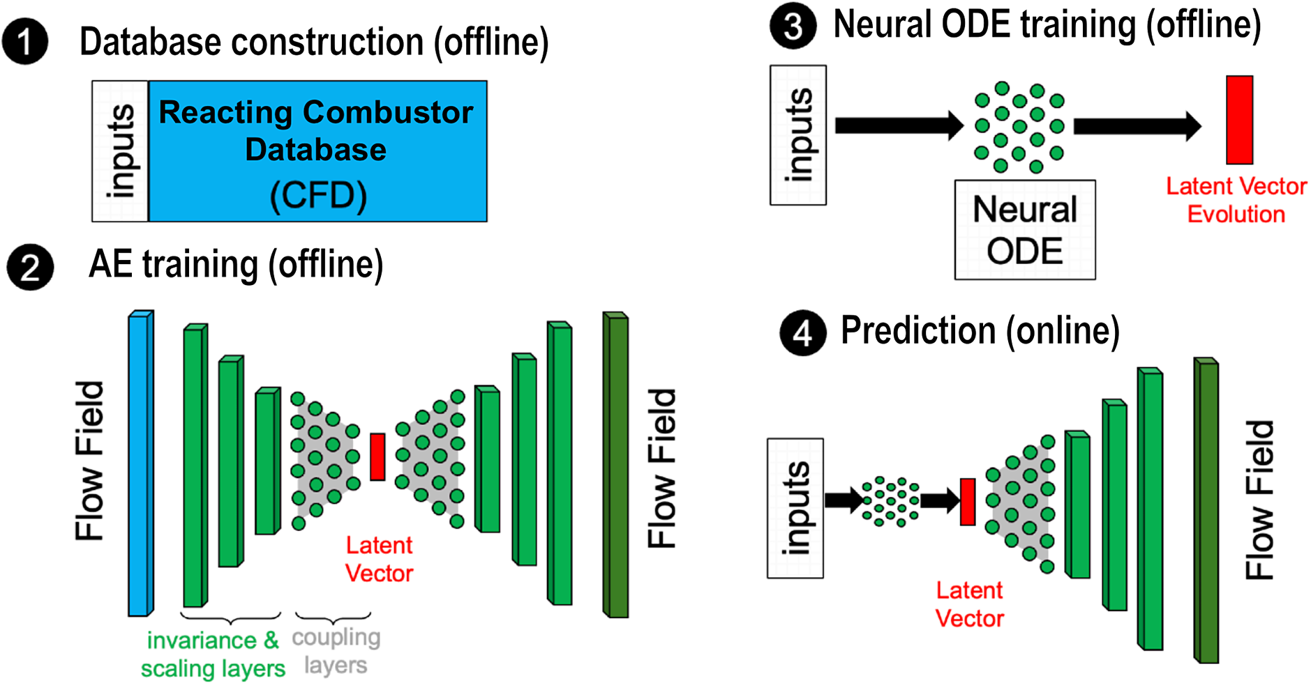
Figure 1. Long description
The flowchart is divided into four numbered panels.
Panel 1. Database construction offline. A white box labeled inputs points into a large blue box labeled Reacting Combustor Database C F D.
Panel 2. A E training offline. A blue vertical bar labeled Flow Field enters a series of green invariance and scaling layers that decrease in size. These lead into gray triangular coupling layers containing green dots, which converge on a central red rectangle labeled Latent Vector. The process then mirrors outward through coupling layers and scaling layers to a final green vertical bar labeled Flow Field.
Panel 3. Neural O D E training offline. A white box labeled inputs points to a cluster of green dots labeled Neural O D E. An arrow from this cluster points to a red rectangle labeled Latent Vector Evolution.
Panel 4. Prediction online. A white box labeled inputs points to a small cluster of green dots, which leads to a red Latent Vector. This vector feeds into the expanding half of the decoder from panel 2, consisting of gray coupling layers and green scaling layers, terminating at a final green vertical bar labeled Flow Field.
2. Data and methodology
2.1. Sources of uncertainty and data representation
The ensemble of LES ignition trials described in Section 1 provides a data-driven view of how different operating conditions lead to ignition success or failure. To interpret and generalize these outcomes, we formalize the system variability within a structured uncertainty quantification (UQ) campaign (Cutforth et al., Reference Cutforth, Fan, Zahtila, Doostan and Darve2026). This framework identifies 15 input parameters (summarized in Table A1 in Appendix A) that encode variability (i.e., uncertainty) originating from the companion experimental campaign, the combustor system, and model-form assumptions. Specifically, the bounds on these parameters were obtained either from direct measurements in the reacting combustor experimental campaign (Strelau et al., Reference Strelau, Frederick, Winter, Senior, Gejji and Slabaugh2024), or from detailed simulations of a laser spark matched to quiescent combustor experiments (Brouzet et al., Reference Brouzet, Zahtila, Rossinelli, Voci, Iaccarino, Passiatore, Strelau, Gejji and Slabaugh2025), from which the laser parameters were statistically inferred from the spark evolution. The remaining parameters were treated as model-form uncertainties and assigned narrow prior ranges to guard against overlooked sensitivities in the ignition response. These inputs form the parametric drivers for the surrogate model. Briefly, the uncertainty set includes epistemic variations in laser spark characteristics and focal accuracy (
$ {\xi}_0 $
 –
$ {\xi}_5 $
–
$ {\xi}_5 $
 ). Deposition timing is influenced by two distinct mechanisms: (a) small-scale lags that introduce aleatoric uncertainty through turbulence-driven shifts (
$ {\xi}_6 $
). Deposition timing is influenced by two distinct mechanisms: (a) small-scale lags that introduce aleatoric uncertainty through turbulence-driven shifts (
$ {\xi}_6 $
 ) and (b) large-scale lags that capture epistemic uncertainty due to variability in the available methane system mass (
$ {\xi}_7 $
) and (b) large-scale lags that capture epistemic uncertainty due to variability in the available methane system mass (
$ {\xi}_7 $
 ). Additional sources include modeling uncertainties in flame propagation (
$ {\xi}_8 $
). Additional sources include modeling uncertainties in flame propagation (
$ {\xi}_8 $
 –
$ {\xi}_{10} $
–
$ {\xi}_{10} $
 ), model-form uncertainty in the subgrid stress coefficient (
$ {\xi}_{11} $
), model-form uncertainty in the subgrid stress coefficient (
$ {\xi}_{11} $
 ), epistemic uncertainties tied to fuel–oxidizer intake conditions (
$ {\xi}_{12} $
), epistemic uncertainties tied to fuel–oxidizer intake conditions (
$ {\xi}_{12} $
 –
$ {\xi}_{13} $
–
$ {\xi}_{13} $
 ), and geometric variability in combustor cross-section (
$ {\xi}_{14} $
), and geometric variability in combustor cross-section (
$ {\xi}_{14} $
 ). The subsequent ignition trial computations were generated by Monte Carlo sampling of the 15-dimensional uncertain input space, with each parameter drawn from its prescribed marginal distribution and treated as statistically independent. Each ignition trial is an LES simulation of a compressible reacting subscale rocket combustor with the Hypersonics Task-based Research (HTR) solver (Di Renzo et al., Reference Di Renzo, Fu and Urzay2020), in which an O
$ {}_2 $
). The subsequent ignition trial computations were generated by Monte Carlo sampling of the 15-dimensional uncertain input space, with each parameter drawn from its prescribed marginal distribution and treated as statistically independent. Each ignition trial is an LES simulation of a compressible reacting subscale rocket combustor with the Hypersonics Task-based Research (HTR) solver (Di Renzo et al., Reference Di Renzo, Fu and Urzay2020), in which an O
$ {}_2 $
 -CH
$ {}_4 $
-CH
$ {}_4 $
 coflowing injector jet develops into a chamber. After development of the preignition turbulent state, a laser spark deposits an energy kernel whose subsequent evolution and interaction with the turbulent coflowing jet determine whether ignition succeeds or fails. The cost of one simulation is a wall-clock time of
$ \mathcal{O} $
coflowing injector jet develops into a chamber. After development of the preignition turbulent state, a laser spark deposits an energy kernel whose subsequent evolution and interaction with the turbulent coflowing jet determine whether ignition succeeds or fails. The cost of one simulation is a wall-clock time of
$ \mathcal{O} $
 (10) hours on 8 NVIDIA V100 GPU cards, which is a significant reduction relative to the high-fidelity simulation counterpart, achieved through reduced chemistry and strategic meshing together with tuning of deterministic features such as the jet inviscid core and spark evolution at common sample points. A detailed account of the simulations flow rates, timings, and combustor geometry is provided in the corresponding high-fidelity simulation campaign (Brouzet et al., Reference Brouzet, Rossinelli, Zahtila, Voci, Strelau, Warner, Gejji, Slabaugh and Iaccarino2026).
A central aim of the UQ campaign was to assess ignition sensitivities in the combustor, and each of the LES computations in the ensemble of ignition trials leads to a response of ignition failure or success. To this end, Figure 2 shows marginal distributions of the input parameters, separated into igniting and nonigniting cases. While some distributions differ only slightly (reflecting sampling convergence), others exhibit clear structural differences. To quantify these differences, the Kullback–Leibler (KL) divergence (Kullback and Leibler, Reference Kullback and Leibler1951) was computed between the success and failure groups, with parameters exhibiting the largest divergence highlighted in Figure 2 with green check marks. To complement the KL-based marginal comparison, we also evaluated conditional Sobol sensitivities using a random-forest ignition classifier. In a preliminary analysis,
$ {\xi}_7 $
 (methane system mass) was found to be dominant, followed by the same leading parameters highlighted by the KL analysis; however, the strong influence of
$ {\xi}_7 $
(methane system mass) was found to be dominant, followed by the same leading parameters highlighted by the KL analysis; however, the strong influence of
$ {\xi}_7 $
 reduced the ability of the Sobol analysis to clearly resolve secondary interaction effects among the remaining inputs. Accordingly,
$ {\xi}_7 $
reduced the ability of the Sobol analysis to clearly resolve secondary interaction effects among the remaining inputs. Accordingly,
$ {\xi}_7 $
 was fixed and the Sobol sensitivities were recomputed over the remaining input space. In this conditional analysis,
$ {\xi}_2 $
was fixed and the Sobol sensitivities were recomputed over the remaining input space. In this conditional analysis,
$ {\xi}_2 $
 (lobe asymmetry ratio) and
$ {\xi}_5 $
(lobe asymmetry ratio) and
$ {\xi}_5 $
 (energy deposited) remained the leading contributors, with first-order indices
$ {S}_1=0.54\pm 0.06 $
(energy deposited) remained the leading contributors, with first-order indices
$ {S}_1=0.54\pm 0.06 $
 and
$ 0.24\pm 0.05 $
and
$ 0.24\pm 0.05 $
 , respectively. The largest pairwise interaction was
$ \left({\xi}_2,{\xi}_5\right) $
, respectively. The largest pairwise interaction was
$ \left({\xi}_2,{\xi}_5\right) $
 , with
$ {S}_2=0.06\pm 0.08 $
, with
$ {S}_2=0.06\pm 0.08 $
 , where the confidence bounds were estimated by bootstrap resampling of the surrogate model evaluations. These statistical trends have a clear physical interpretation. Increasing the deposited laser energy (
$ {\xi}_5 $
, where the confidence bounds were estimated by bootstrap resampling of the surrogate model evaluations. These statistical trends have a clear physical interpretation. Increasing the deposited laser energy (
$ {\xi}_5 $
 ) produces a larger ignition kernel, making it more likely to overcome turbulent transport cooling and breakup (Passiatore et al., Reference Passiatore, Wang, Rossinelli, Di Renzo and Iaccarino2024). Increasing the methane system mass (
$ {\xi}_7 $
) produces a larger ignition kernel, making it more likely to overcome turbulent transport cooling and breakup (Passiatore et al., Reference Passiatore, Wang, Rossinelli, Di Renzo and Iaccarino2024). Increasing the methane system mass (
$ {\xi}_7 $
 ) increases the fuel available to the evolving kernel and improves the chance of sustained flame growth in locally favorable mixture regions. The
$ {\xi}_2 $
) increases the fuel available to the evolving kernel and improves the chance of sustained flame growth in locally favorable mixture regions. The
$ {\xi}_2 $
 –
$ {\xi}_5 $
–
$ {\xi}_5 $
 interaction reflects the coupled role of spark structure and spark strength:
$ {\xi}_5 $
interaction reflects the coupled role of spark structure and spark strength:
$ {\xi}_5 $
 sets the kernel energy, while
$ {\xi}_2 $
sets the kernel energy, while
$ {\xi}_2 $
 influences the laser-spark asymmetry and hence its propagation toward favorable chemistry (Wang et al., Reference Wang, Buchta and Freund2020). However, ignition is fundamentally a Bernoulli random variable (success/failure), even if a continuous proxy is used, e.g., the maximum chamber pressure over time instead of a Boolean label. The underlying problem of predicting a sharp regime transition between ignition and failure is not removed by the proxy. Consequently, reliable probability estimates are slow to converge. For example, with only
$ N=100 $
influences the laser-spark asymmetry and hence its propagation toward favorable chemistry (Wang et al., Reference Wang, Buchta and Freund2020). However, ignition is fundamentally a Bernoulli random variable (success/failure), even if a continuous proxy is used, e.g., the maximum chamber pressure over time instead of a Boolean label. The underlying problem of predicting a sharp regime transition between ignition and failure is not removed by the proxy. Consequently, reliable probability estimates are slow to converge. For example, with only
$ N=100 $
 independent trials and a nominal ignition probability of
$ p=0.5 $
independent trials and a nominal ignition probability of
$ p=0.5 $
 , the Wilson score interval (Wilson, Reference Wilson1927) still gives an uncertainty range of approximately
$ \left[\mathrm{0.40,0.60}\right] $
, the Wilson score interval (Wilson, Reference Wilson1927) still gives an uncertainty range of approximately
$ \left[\mathrm{0.40,0.60}\right] $
 , highlighting the substantial sampling uncertainty associated with limited LES ensembles. Given finite compute allocations and therefore limited sampling, the available LES ensemble is insufficient for robust convergence, and this motivates the construction of the DnAE surrogate model to efficiently augment ignition probability quantification. A comprehensive joint characterization of the most informative parameters is deferred; we return to it later using surrogate-enabled Monte Carlo.
Ignition probability density functions (PDFs) marginalized over the input parameters
$ {\xi}_0 $
 through
$ {\xi}_{14} $
through
$ {\xi}_{14} $
 , comparing ignition success (red) and ignition failure (blue) through kernel density estimates; green check marks denote the five parameters with the largest KL divergence between igniting and nonigniting cases. Full description of parameters in Table A1 in Appendix A.
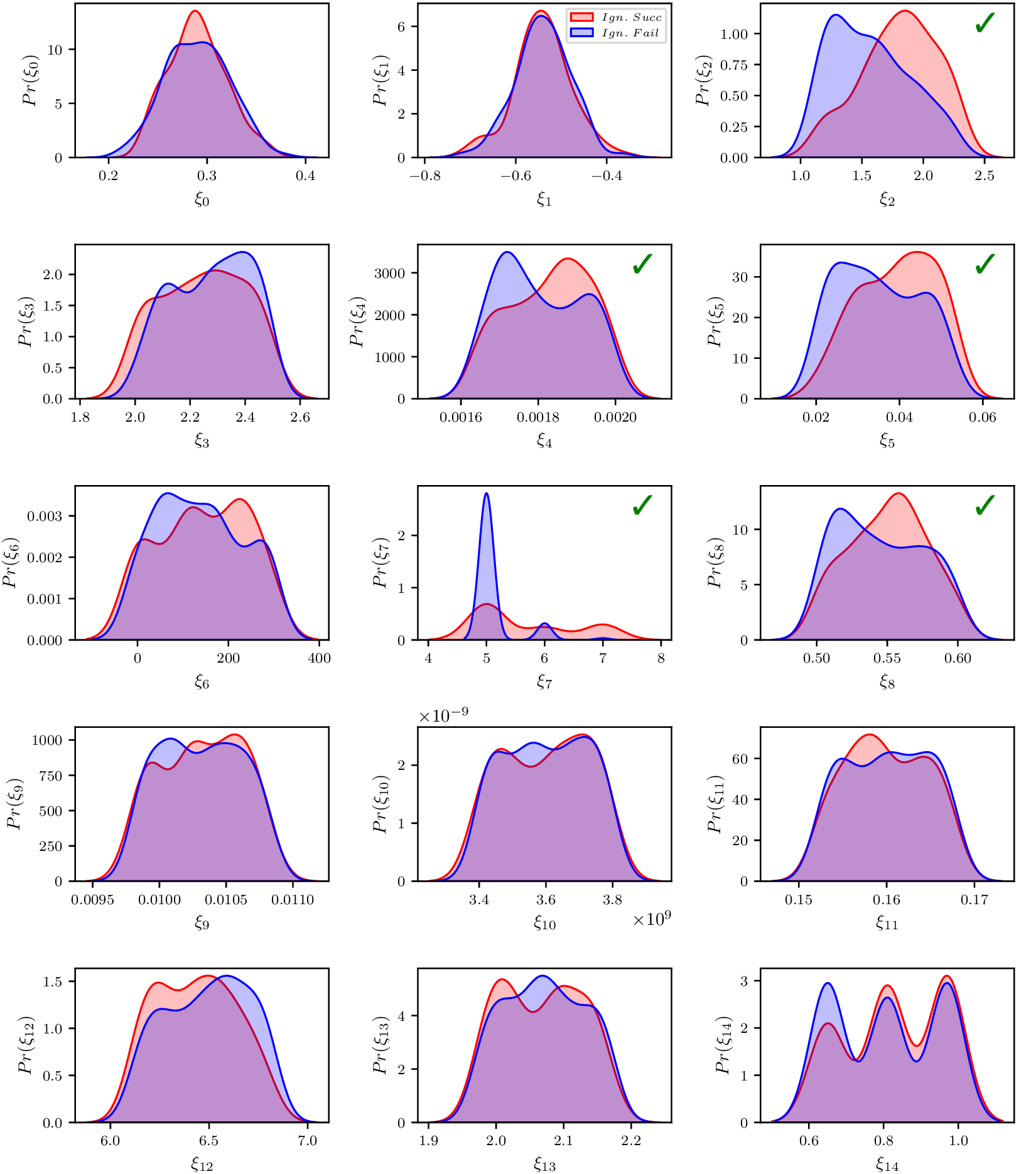
Figure 2. Long description
The grid contains 5 rows and 3 columns of kernel density estimate plots. Each plot features two overlapping shaded regions: red for ignition success and blue for ignition failure.
* Row 1: xi sub 0 shows nearly identical bell curves centered at 0.3. xi sub 1 shows overlapping curves centered at negative 0.55. xi sub 2 shows a significant shift where success peaks at 1.8 and failure peaks at 1.3, marked with a green check.
* Row 2: xi sub 3 shows overlapping bimodal distributions. xi sub 4 shows success peaking at 0.0019 and failure at 0.0017, marked with a green check. xi sub 5 shows success peaking at 0.045 and failure at 0.025, marked with a green check.
* Row 3: xi sub 6 shows broad overlapping distributions. xi sub 7 shows a sharp failure peak at 5.0 while success is distributed across 5.0, 6.0, and 7.0, marked with a green check. xi sub 8 shows success peaking at 0.56 and failure at 0.52, marked with a green check.
* Row 4: xi sub 9, xi sub 10, and xi sub 11 all show highly similar, multi-modal overlapping distributions for both success and failure.
* Row 5: xi sub 12, xi sub 13, and xi sub 14 continue the trend of high overlap with minor variations in peak heights across the parameter ranges.
The green check marks in panels xi sub 2, xi sub 4, xi sub 5, xi sub 7, and xi sub 8 highlight the parameters where the red and blue distributions differ most significantly.
To assemble a statistically useful LES dataset for reduced order modeling, we generated
$ {N}_c=300 $
 ignition trials by first constructing tailored LES (Cutforth et al., Reference Cutforth, Fan, Zahtila, Doostan and Darve2026) built from large-scale experimentally validated calculations (Passiatore et al., Reference Passiatore, Wang, Rossinelli, Di Renzo and Iaccarino2024; Brouzet et al., Reference Brouzet, Zahtila, Rossinelli, Voci, Iaccarino, Passiatore, Strelau, Gejji and Slabaugh2025). The tailored LES computations differ from the increased scale-resolving calculations, for which
$ \mathcal{O}\left(1-10\right) $
ignition trials by first constructing tailored LES (Cutforth et al., Reference Cutforth, Fan, Zahtila, Doostan and Darve2026) built from large-scale experimentally validated calculations (Passiatore et al., Reference Passiatore, Wang, Rossinelli, Di Renzo and Iaccarino2024; Brouzet et al., Reference Brouzet, Zahtila, Rossinelli, Voci, Iaccarino, Passiatore, Strelau, Gejji and Slabaugh2025). The tailored LES computations differ from the increased scale-resolving calculations, for which
$ \mathcal{O}\left(1-10\right) $
 are feasible, because they employ a significantly coarser mesh and feature reduced chemistry and are calibrated by employing an Ensemble Kalman filter (EnKF) for deterministic processes. This procedure matched the tailored LES to emulate the high-fidelity deterministic processes in the laser kernel dynamics and turbulence quantities in the coflowing jet. With this calibration in place, larger ensembles became feasible. The choice of
$ {N}_c=300 $
are feasible, because they employ a significantly coarser mesh and feature reduced chemistry and are calibrated by employing an Ensemble Kalman filter (EnKF) for deterministic processes. This procedure matched the tailored LES to emulate the high-fidelity deterministic processes in the laser kernel dynamics and turbulence quantities in the coflowing jet. With this calibration in place, larger ensembles became feasible. The choice of
$ {N}_c=300 $
 trials was guided by computational cost constraints and the convergence of the cumulative ignition-probability estimate, with the estimate
$ {\hat{P}}_{\mathrm{ign}} $
trials was guided by computational cost constraints and the convergence of the cumulative ignition-probability estimate, with the estimate
$ {\hat{P}}_{\mathrm{ign}} $
 stabilizing to within
$ \pm 5\% $
stabilizing to within
$ \pm 5\% $
 after
$ {N}_c=300 $
after
$ {N}_c=300 $
 samples. The resulting dataset enabled the construction of ignition probability maps. Logistic fits of ignition probability as a function of radial focal position were consistent with the experimental probability maps in both the mean prediction and the 95% confidence interval, indicating statistical agreement between the computational ensemble data and the laboratory model rocket-combustor experiments (Strelau et al., Reference Strelau, Frederick, Winter, Senior, Gejji and Slabaugh2024).
2.2. Quantity of interest: thermal imaging
Having generated a large and statistically useful tailored LES data ensemble, we proceed to select an appropriate representation of the combustor dynamics on which to train and develop the surrogate model. In this predictive rocket-ignition context, we therefore require a reduced data representation that remains physically meaningful yet tractable for learning. A further requirement for validation would be that the representation is relatable to the observables from experimental sensing modalities. Machine learning surrogate models trained on reduced or structure-promoting representations are preferable in turbulence due to the extremely high dimensionality, chaotic nature, and multiscale features of full 3D fields. Recent examples include, in the context of multiphase flows, investigation on the choice of interface treatment through diffuse, sharp, and level set approaches (Cutforth and Mirjalili, Reference Cutforth and Mirjalili2025), and in urban street canyons, 2D particle image velocimetry was preferable at a judiciously chosen plane that captured turbulence quadrant events (Jaroslawski et al., Reference Jaroslawski, Patil and McKeon2025). These reduced forms capture essential dynamics while significantly lowering computational cost and mitigating overfitting, making learning more tractable and generalizable. The essential features in the combustor include (1) coflowing (fuel and oxidizer) turbulent intake, (2) deposited energy kernel location and dynamics, and in the successful ignition scenario, (3) flame propagation and stable combustion.
Figure 3(a) displays rendered output from the computational fluid dynamics (CFD) solver (Di Renzo et al., Reference Di Renzo, Fu and Urzay2020) and the associated flame visualization. To emulate the experimental data acquisition, our first approach is to computationally emulate high-speed Schlieren by integrating light beams for a collimated light source passing through the variable density flow. The trajectories obey the governing equation derived from Fermat’s principle:
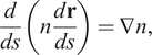
where
$ \mathbf{r}(s) $
 is the light-beam trajectory parameterized by arc length
$ s $
is the light-beam trajectory parameterized by arc length
$ s $
 , and
$ n $
, and
$ n $
 is the refractive-index field calculated from the species mass fractions and Gladstone–Dale mixture relation, with full details in supplementary material of high-fidelity simulations (Brouzet et al., Reference Brouzet, Rossinelli, Zahtila, Voci, Strelau, Warner, Gejji, Slabaugh and Iaccarino2026), as part of a wider paradigm of digital enhancement of flow data (Rossinelli et al., Reference Rossinelli, Hu, Marshall, Kozak, Zahtila, Brouzet, Cutforth, Mungal and Iaccarino2026a,Reference Rossinelli, Li, Voci, Marshall, Hu, Brouzet, Fan, Williams, Martin, Khanwale, Vignat, Zahtila, Cutforth and Iaccarinob). The path-tracing approach illustrated in Figure 3(b) mimics experimental line-of-sight integration to reduce the data to a 2D field quantity. While informative, this high-dimensional representation includes numerous flow and combustion features that are not necessarily predictive of ignition success.
Quantity of interest: spatiotemporal fields, (a) rendered simulation output of the successfully ignited combustor, (b) illustration of the integrated quantity acquisition, (1) light beam generation, (2) ray evolution according to the Eikonal equation, (3) Snell’s law and occlusion, and (4) irradiance sampling, (c) successful and unsuccessful time series for the computational infrared representation, and (d) computational Schlieren.
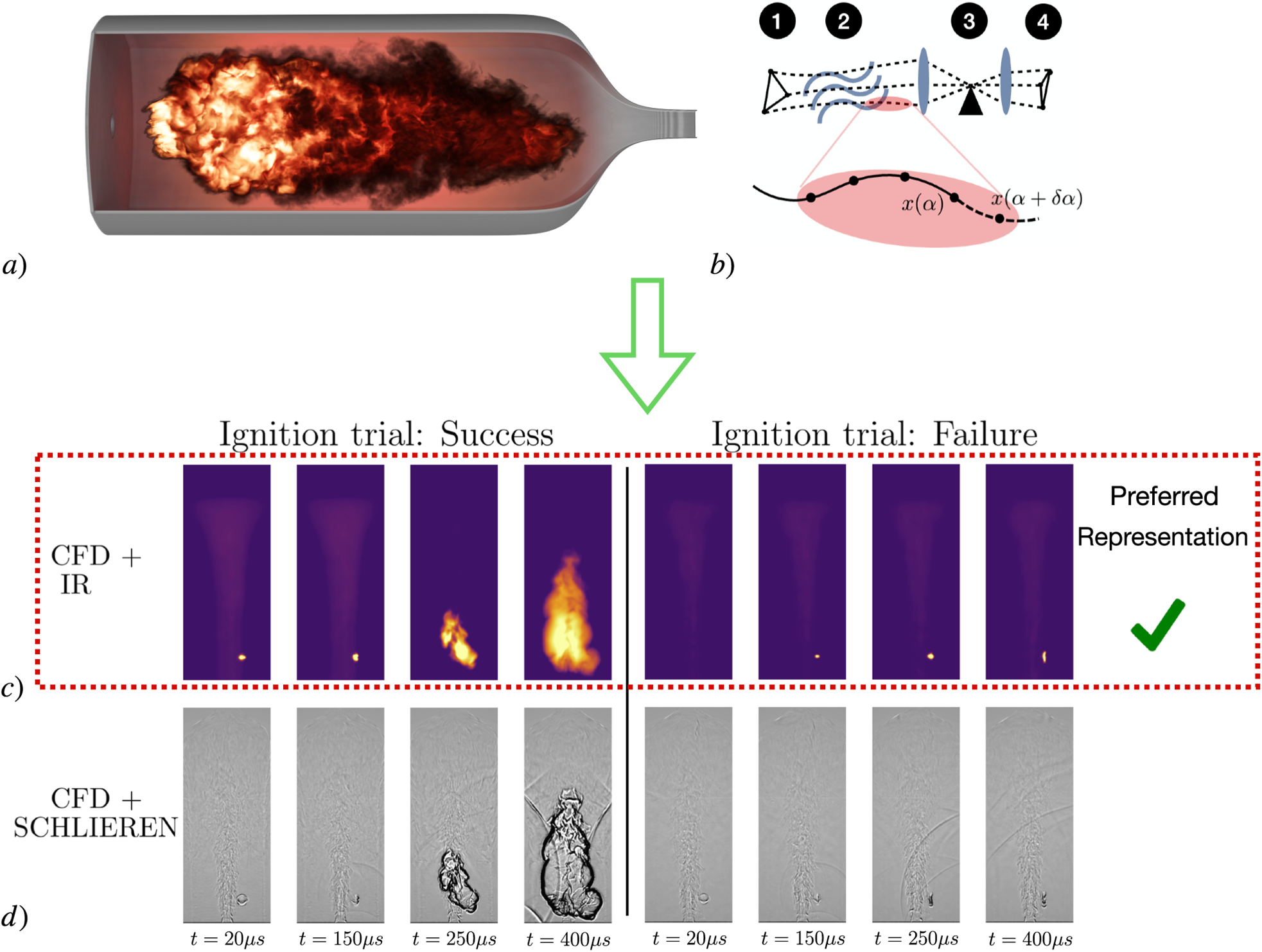
Figure 3. Long description
The image is divided into four sections labeled a through d.
* Panel a: A cross-sectional rendering of a cylindrical combustor containing a turbulent, orange and black flame plume during a successful ignition event.
* Panel b: A schematic of light beam evolution. It includes four numbered stages: 1 shows light beam generation from a source; 2 shows ray evolution through wavy blue lines; 3 depicts a lens and an occlusion point marked by a black triangle; 4 shows irradiance sampling at a detector. A callout below shows a curved path with points x alpha and x open parenthesis alpha plus delta alpha close parenthesis.
* Panel c: A horizontal sequence of eight vertical heat maps labeled C F D plus I R. The left four panels show a successful ignition trial where a bright yellow flame kernel grows from t equals 20 mu s to t equals 400 mu s. The right four panels show a failed trial where the kernel remains small and dissipates. This row is enclosed in a red dotted box labeled Preferred Representation with a green checkmark.
* Panel d: A horizontal sequence of eight grayscale images labeled C F D plus SCHLIEREN corresponding to the same time steps as panel c. The successful trial on the left shows expanding shockwaves and density gradients that form a large plume by 400 mu s, while the failed trial on the right shows only faint, dissipating waves.
The computational infrared (IR) imaging emulates the methodology used for chemiluminescence modeling (Brouzet et al., Reference Brouzet, Rossinelli, Zahtila, Voci, Strelau, Warner, Gejji, Slabaugh and Iaccarino2026) and instead of integrating refractive beam trajectories, this method relies on the orthographic projection of a volumetric emission field. While the chemiluminescence model utilizes species concentrations to define the source term, radiative emission is modeled to reproduce thermal imaging from the temperature field. Representative time series for both successful and failed ignition events are shown using IR imagery in Figure 3(c) and computational Schlieren imaging in Figure 3(d). Although the Schlieren images capture a wide range of turbulent spatial scales, we prioritized the CFD IR representation due to its more informative representation of spark location and subsequent dynamical evolution of the laser-deposited energy kernel. For the conducted
$ {N}_c=300 $
 CFD cases, we generated
$ {N}_t=20 $
CFD cases, we generated
$ {N}_t=20 $
 aligned postdeposition IR snapshots per case. This resolution captured the essential kernel dynamics and combustion evolution while balancing memory requirements to fit the resultant data matrix on a single graphical processing unit (GPU).
2.3. Autoencoder
Despite the spatial reduction from 3D to 2D through integrated quantities, the IR fields described in §2.2 must be further reduced in dimensionality in order to enable temporal modeling in the first place. We choose nonlinear convolutional autoencoders (cAEs) because they have been demonstrated to yield efficient compression while retaining essential physical structures (Saetta et al., Reference Saetta, Tognaccini and Iaccarino2024b); however, alternative approaches for learning latent manifolds are also available (Fan et al., Reference Fan, Cutforth, D’Elia, Cortiella, Doostan and Darve2025; Lu et al., Reference Lu, Lam and Zahtila2026). In the present framework, we therefore employ a cAE that learns a low-dimensional latent representation using an architecture composed of three convolutional blocks that progressively extract multiscale spatial features while reducing resolution. These blocks utilize increasing channel counts and intervening pooling operations, augmented with residual connections and nonlinear activation functions. Subsequently, fully connected layers nonlinearly combine these multiresolution features to compress the
$ \mathbf{x}\in {\unicode{x211D}}^{592\times 240} $
 input IR fields to an eight-dimensional latent state
$ \mathbf{V} $
input IR fields to an eight-dimensional latent state
$ \mathbf{V} $
 . Finally, the decoder mirrors this configuration, employing symmetric upsampling and convolutional blocks to reconstruct the full high-resolution input space from
$ \mathbf{V} $
. Finally, the decoder mirrors this configuration, employing symmetric upsampling and convolutional blocks to reconstruct the full high-resolution input space from
$ \mathbf{V} $
 , see Figure 4(a,c).
Architecture schematic for the DnAE. (a) The encoder maps each single-channel IR field to an 8-dimensional latent state
$ \mathbf{V} $
 using convolutional, pooling, residual, and fully connected layers. (b) The NODE represents the latent-space right-hand side: at each integration step, the augmented state
$ \left(\mathbf{V},\boldsymbol{\xi}, t\right) $
using convolutional, pooling, residual, and fully connected layers. (b) The NODE represents the latent-space right-hand side: at each integration step, the augmented state
$ \left(\mathbf{V},\boldsymbol{\xi}, t\right) $
 is passed through two fully connected layers to evaluate the latent space derivative. Repeated evaluations within the time integrator advance the latent trajectory over the ignition trial. (c) The decoder maps
$ \mathbf{V} $
is passed through two fully connected layers to evaluate the latent space derivative. Repeated evaluations within the time integrator advance the latent trajectory over the ignition trial. (c) The decoder maps
$ \mathbf{V} $
 back to image space using fully connected, upsampling, and convolutional layers.
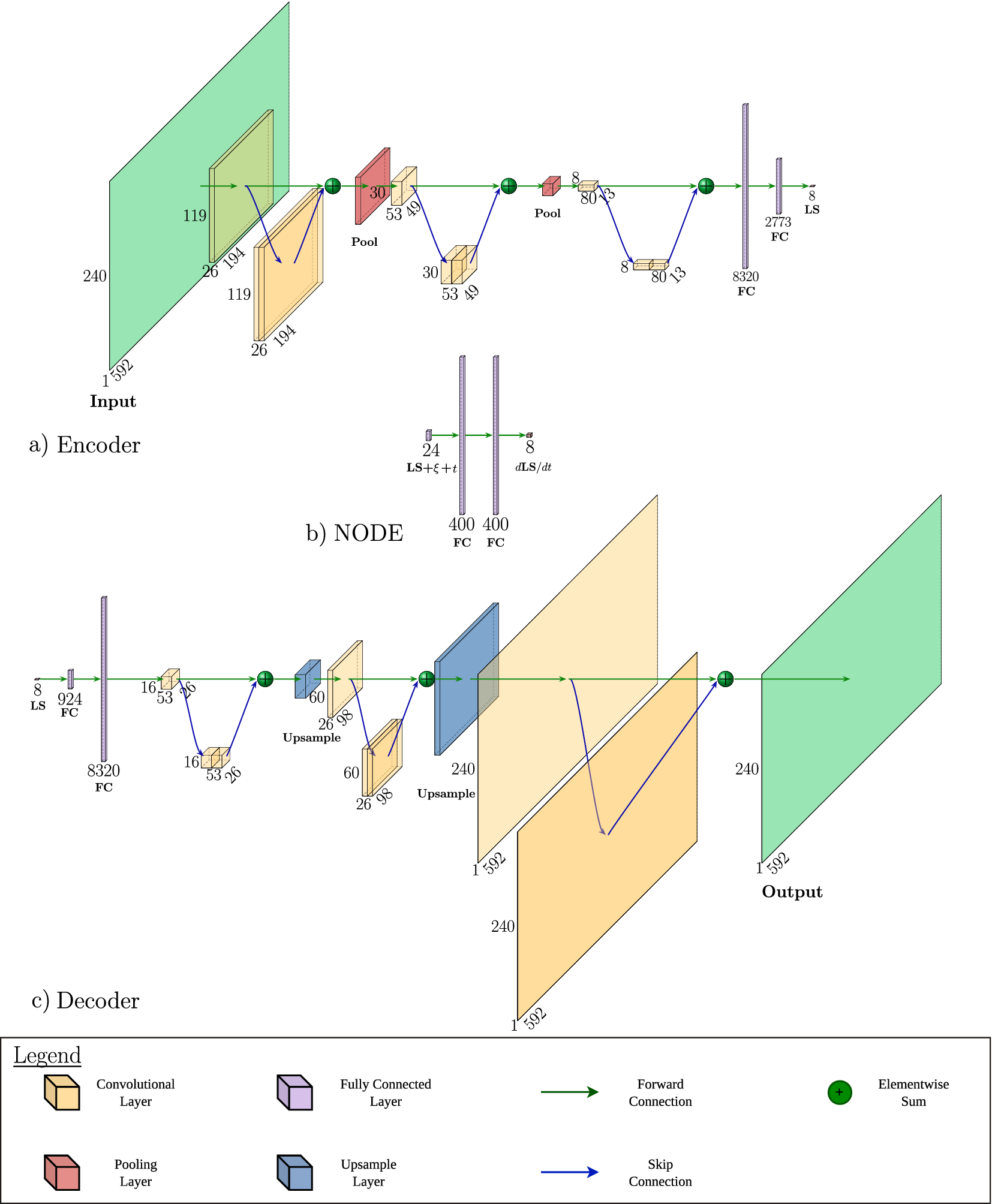
Figure 4. Long description
The schematic is divided into three main sections and a legend.
Panel a, Encoder. Data flows from a green input plane (240 by 592) through a series of yellow convolutional and red pooling layers. Blue skip connection arrows bypass certain layers to join green elementwise sum nodes. The process concludes with two purple F C (Fully Connected) layers of sizes 8320 and 2773, resulting in an 8-dimensional L S (Latent State).
Panel b, N O D E. This central section shows the latent state plus xi plus t (size 24) entering two purple F C layers of size 400 each. The output is the derivative d L S / d t (size 8).
Panel c, Decoder. The 8-dimensional L S enters a 924-unit F C layer, followed by an 8320-unit F C layer. The data then passes through yellow convolutional and blue upsampling layers. Similar to the encoder, blue skip connections link earlier layers to later elementwise sum nodes. The final output is a green plane (240 by 592).
Legend at the bottom defines the components.
* Yellow cube: Convolutional Layer.
* Red cube: Pooling Layer.
* Purple vertical bar: Fully Connected Layer.
* Blue cube: Upsample Layer.
* Green arrow: Forward Connection.
* Blue arrow: Skip Connection.
* Green circle with plus sign: Elementwise Sum.
As a preprocessing step, each image matrix is min–max normalized to the range
$ \left[0,1\right] $
 through affine rescaling, ensuring consistent numerical scale and improved conditioning during training (LeCun et al., Reference LeCun, Bottou, Orr and Müller2012). Each normalized light–intensity field is passed to the AE as a single-channel 2D input, on which the network performs a nonlinear encoding–decoding operation:

where
$ e:{\unicode{x211D}}^{m\times n}\to {\unicode{x211D}}^{N_{\mathrm{\ell}}} $
 is the encoder mapping for an input with dimensions
$ m\times n $
is the encoder mapping for an input with dimensions
$ m\times n $
 , and
$ d:{\unicode{x211D}}^{N_{\mathrm{\ell}}}\to {\unicode{x211D}}^{m\times n} $
, and
$ d:{\unicode{x211D}}^{N_{\mathrm{\ell}}}\to {\unicode{x211D}}^{m\times n} $
 the decoder mapping. Here,
$ \mathbf{x} $
the decoder mapping. Here,
$ \mathbf{x} $
 denotes the input field,
$ \hat{\mathbf{x}} $
denotes the input field,
$ \hat{\mathbf{x}} $
 its reconstruction, and
$ \mathbf{V}\in {\unicode{x211D}}^{N_{\mathrm{\ell}}} $
its reconstruction, and
$ \mathbf{V}\in {\unicode{x211D}}^{N_{\mathrm{\ell}}} $
 the latent variables. Following Saetta et al. (Reference Saetta, Tognaccini and Iaccarino2022), the optimization objective is a regularized reconstruction loss

where
$ {\mathbf{x}}_i $
 is the
$ i $
is the
$ i $
 th AE training snapshot, sampled from any training ignition case and any available time snapshot,
$ {\hat{\mathbf{x}}}_i $
th AE training snapshot, sampled from any training ignition case and any available time snapshot,
$ {\hat{\mathbf{x}}}_i $
 is its reconstruction,
$ N $
is its reconstruction,
$ N $
 is the total number of AE training snapshots,
$ {l}_q^e $
is the total number of AE training snapshots,
$ {l}_q^e $
 denotes the
$ q $
denotes the
$ q $
 th encoder weight,
$ {N}_e $
th encoder weight,
$ {N}_e $
 is the total number of encoder weights, and
$ {\lambda}_{\mathrm{AE}} $
is the total number of encoder weights, and
$ {\lambda}_{\mathrm{AE}} $
 is a user-defined regularization coefficient. In our implementation, we set
$ {\lambda}_{\mathrm{AE}}={10}^{-6} $
is a user-defined regularization coefficient. In our implementation, we set
$ {\lambda}_{\mathrm{AE}}={10}^{-6} $
 for
$ {L}_2 $
for
$ {L}_2 $
 autoencoder regularization, consistent with prior work on aerodynamic AEs. The latent space dimension
$ {N}_{\mathrm{\ell}} $
autoencoder regularization, consistent with prior work on aerodynamic AEs. The latent space dimension
$ {N}_{\mathrm{\ell}} $
 is a critical hyperparameter that controls the latent-space manifold capturing the essential flow physics.
A key property of this construction is that the AE is deterministic: for any unseen input
$ \mathbf{x} $
 , the encoder yields a unique latent vector
$ \mathbf{V}=e\left(\mathbf{x}\right) $
, the encoder yields a unique latent vector
$ \mathbf{V}=e\left(\mathbf{x}\right) $
 , which the decoder deterministically maps back to the reconstructed field
$ \hat{\mathbf{x}}=d\left(\mathbf{V}\right) $
, which the decoder deterministically maps back to the reconstructed field
$ \hat{\mathbf{x}}=d\left(\mathbf{V}\right) $
 . In contrast to variational autoencoder (VAE) approaches that introduce stochasticity in the latent space (Fan et al., Reference Fan, Cutforth, D’Elia, Cortiella, Doostan and Darve2025), this deterministic structure ensures reproducibility of trajectories and avoids additional assumptions on the latent distribution (Saetta et al., Reference Saetta, Tognaccini and Iaccarino2024b). In steady-state settings, once the latent space is established, the decoder can be deployed as a generative model by interpolating within the latent manifold (Saetta et al., Reference Saetta, Tognaccini and Iaccarino2024b). For example, new realizations may be generated as
$ \mathbf{V}\left(\boldsymbol{\xi} \right)=\mathcal{I}\left(\boldsymbol{\xi}; {\left\{\left({\boldsymbol{\xi}}^{(j)},{\mathbf{V}}^{(j)}\right)\right\}}_{j=1}^{N_c}\right) $
. In contrast to variational autoencoder (VAE) approaches that introduce stochasticity in the latent space (Fan et al., Reference Fan, Cutforth, D’Elia, Cortiella, Doostan and Darve2025), this deterministic structure ensures reproducibility of trajectories and avoids additional assumptions on the latent distribution (Saetta et al., Reference Saetta, Tognaccini and Iaccarino2024b). In steady-state settings, once the latent space is established, the decoder can be deployed as a generative model by interpolating within the latent manifold (Saetta et al., Reference Saetta, Tognaccini and Iaccarino2024b). For example, new realizations may be generated as
$ \mathbf{V}\left(\boldsymbol{\xi} \right)=\mathcal{I}\left(\boldsymbol{\xi}; {\left\{\left({\boldsymbol{\xi}}^{(j)},{\mathbf{V}}^{(j)}\right)\right\}}_{j=1}^{N_c}\right) $
 , where
$ \mathcal{I} $
, where
$ \mathcal{I} $
 denotes an interpolation operator acting on the latent ensemble and associated input parameters, yielding
$ \hat{\mathbf{x}}\left(\boldsymbol{\xi} \right)=d\left(\mathbf{V}\left(\boldsymbol{\xi} \right)\right) $
denotes an interpolation operator acting on the latent ensemble and associated input parameters, yielding
$ \hat{\mathbf{x}}\left(\boldsymbol{\xi} \right)=d\left(\mathbf{V}\left(\boldsymbol{\xi} \right)\right) $
 . For the present unsteady ignition problem, this idea is extended by learning the temporal evolution of the latent state with a parameterized neural ODE, rather than interpolating the full latent trajectory directly. Thus, the decoder remains the generative map from latent space to image space, while the NODE supplies the time-dependent latent trajectory.
2.4. Parameterized neural ODE
The temporal dynamics of the latent space representation
$ {\mathbf{V}}^{(j)}(t) $
 for ignition trial
$ j $
for ignition trial
$ j $
 are advanced using a parameterized NODE framework to model the continuous evolution of the latent space variables, which forms a system of coupled ODEs,

where the present model form differs from the vanilla neural ODE shown in (1.1) by the incorporation of the input parameter vector
$ {\boldsymbol{\xi}}^{(j)} $
 , and as a reminder
$ \boldsymbol{\theta} $
, and as a reminder
$ \boldsymbol{\theta} $
 denotes the learnable parameters of the network. The vanilla neural ODE is sufficient, for example, to emulate the latent space dynamics for flow past a cylinder with a single instance of the parameter space (Rojas et al., Reference Rojas, Dengel and Ribeiro2021), but the parameterized extension can account for variations in the input parameters (Lee and Parish, Reference Lee and Parish2021). Instead of introducing uncertainty via a VAE in the preceding dimensionality reduction stage, we handle parametric uncertainty here by conditioning the latent NODE dynamics directly on the input vector
$ \boldsymbol{\xi} $
denotes the learnable parameters of the network. The vanilla neural ODE is sufficient, for example, to emulate the latent space dynamics for flow past a cylinder with a single instance of the parameter space (Rojas et al., Reference Rojas, Dengel and Ribeiro2021), but the parameterized extension can account for variations in the input parameters (Lee and Parish, Reference Lee and Parish2021). Instead of introducing uncertainty via a VAE in the preceding dimensionality reduction stage, we handle parametric uncertainty here by conditioning the latent NODE dynamics directly on the input vector
$ \boldsymbol{\xi} $
 .
.
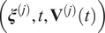
The network in this study is a simple feed-forward network, but additional network features can be added, such as through convolutional layers (Shankar et al., Reference Shankar, Portwood, Mohan, Mitra, Rackauckas, Wilson, Schmidt and Viswanathan2020). Here,
$ f\left(\cdot \right) $
 is a multilayer perceptron with two hidden layers of width
$ w $
is a multilayer perceptron with two hidden layers of width
$ w $
 each with
$ \tanh $
each with
$ \tanh $
 activation, shown within the DnAE in Figure 4(b), mapping the input state
$ \left({\boldsymbol{\xi}}^{(j)},t,{\mathbf{V}}^{(j)}(t)\right) $
activation, shown within the DnAE in Figure 4(b), mapping the input state
$ \left({\boldsymbol{\xi}}^{(j)},t,{\mathbf{V}}^{(j)}(t)\right) $
 to the latent derivatives
$ {\dot{\mathbf{V}}}^{(j)}(t) $
to the latent derivatives
$ {\dot{\mathbf{V}}}^{(j)}(t) $
 . Formally, the latent trajectory for ignition trial
$ j $
. Formally, the latent trajectory for ignition trial
$ j $
 can be written as an initial value problem (Chen et al., Reference Chen, Rubanova, Bettencourt and Duvenaud2018):

which expresses the time series as the initial condition plus the accumulated effect of the latent dynamics. Therefore, given an initial latent state
$ {\mathbf{V}}^{(j)}\left({t}_0\right) $
 from the AE compression for ignition trial
$ j $
from the AE compression for ignition trial
$ j $
 , the NODE-predicted trajectory
$ {\hat{\mathbf{V}}}^{(j)}(t) $
, the NODE-predicted trajectory
$ {\hat{\mathbf{V}}}^{(j)}(t) $
 is propagated from this initial condition over discrete times
$ {\left\{{t}_i\right\}}_{i=0}^{N_t-1} $
is propagated from this initial condition over discrete times
$ {\left\{{t}_i\right\}}_{i=0}^{N_t-1} $
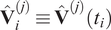
 by
by

where
$ {\Delta}_{\mathrm{RK}4} $
 denotes the fixed-step fourth-order Runge–Kutta increment applied to the parameterized vector field in (2.4),
$ \Delta t={t}_{i+1}-{t}_i $
denotes the fixed-step fourth-order Runge–Kutta increment applied to the parameterized vector field in (2.4),
$ \Delta t={t}_{i+1}-{t}_i $
 ,
$ i $
,
$ i $
 indexes the discrete time snapshots,
$ j $
indexes the discrete time snapshots,
$ j $
 indexes the ignition trial, and
$ {\hat{\mathbf{V}}}_i^{(j)}\equiv {\hat{\mathbf{V}}}^{(j)}\left({t}_i\right) $
indexes the ignition trial, and
$ {\hat{\mathbf{V}}}_i^{(j)}\equiv {\hat{\mathbf{V}}}^{(j)}\left({t}_i\right) $
 . The loss function was specified to enforce trajectory reconstruction accuracy and consistency of temporal derivatives. Specifically,

where
$ {\mathbf{V}}_i^{(j)} $
 is the true latent state for ignition trial
$ j $
is the true latent state for ignition trial
$ j $
 at time snapshot
$ {t}_i $
at time snapshot
$ {t}_i $
 ,
$ {\hat{\mathbf{V}}}_i^{(j)} $
,
$ {\hat{\mathbf{V}}}_i^{(j)} $
 is the corresponding NODE prediction, and
$ {\dot{\mathbf{V}}}_i^{(j)} $
is the corresponding NODE prediction, and
$ {\dot{\mathbf{V}}}_i^{(j)} $
 is a second-order finite-difference approximation of the latent velocity. The weighting hyperparameter
$ {\lambda}_c={10}^{-2} $
is a second-order finite-difference approximation of the latent velocity. The weighting hyperparameter
$ {\lambda}_c={10}^{-2} $
 balances the overall contribution of the temporal-derivative penalty, which is the last term in (2.7). The inclusion of this temporal-derivative penalty is a soft constraint that encourages the neural ODE to learn directional changes, such as those associated with the latent space bifurcation that occurs in ignition.
Briefly, we remark on some present limitations. Separating time and space in our surrogate model’s prediction for evolving temperature fields introduces limitations in their physical consistency. As evolution is handled fully by the neural ODE in a low-dimensional latent state, spatial interactions become effectively nonlocal through the learned AE representation, weakening the system causality. Second, because the latent space itself is not tied to physical conserved quantities, it is difficult to enforce constraints such as conservation laws directly; physics-informed NODE variants such as PINODE (Sholokhov et al., Reference Sholokhov, Liu, Mansour and Nabi2023) partially address this by embedding PDE structure into the dynamics, but they require explicit knowledge of the governing equations, which we do not have for our CFD IR fields.
3. Training
For the bifurcating physics and complex spectrum in rocket ignition and combustion, the effectiveness of the proposed framework relies critically on training methodology; we therefore describe the procedures adopted for the AE and neural ODE to robustly learn the compressed spatial fields and latent trajectories. For both AE and NODE training, the dataset was split by ignition trial into training and validation subsets, with
$ 10\% $
 of the original cases held out for validation. The spatial and temporal components are trained separately to simplify the schedule and, more importantly, joint optimization incurs higher computational cost without necessarily yielding performance gains (Vlachas et al., Reference Vlachas, Arampatzis, Uhler and Koumoutsakos2022). For spatial compression, the encoder reduces the input data matrix
$ \mathcal{S} $
of the original cases held out for validation. The spatial and temporal components are trained separately to simplify the schedule and, more importantly, joint optimization incurs higher computational cost without necessarily yielding performance gains (Vlachas et al., Reference Vlachas, Arampatzis, Uhler and Koumoutsakos2022). For spatial compression, the encoder reduces the input data matrix
$ \mathcal{S} $
 to a compact latent space, and the decoder mirrors this architecture for reconstruction. The immediate output of this stage is therefore a latent coordinate
$ \mathbf{V}=e\left(\mathbf{x}\right) $
to a compact latent space, and the decoder mirrors this architecture for reconstruction. The immediate output of this stage is therefore a latent coordinate
$ \mathbf{V}=e\left(\mathbf{x}\right) $
 for each individual IR snapshot
$ \mathbf{x} $
for each individual IR snapshot
$ \mathbf{x} $
 ; temporal or case-dependent trajectory structure is only imposed subsequently by postprocessing these latent coordinates according to their ignition trial and snapshot index. Confidence in the network design stems from prior work on spatial compression of flow fields (Saetta et al., Reference Saetta, Tognaccini and Iaccarino2022) and preliminary studies therein evaluating the influence of architectural hyperparameters (e.g., number of layers, activation functions). The latent space dimension,
$ {N}_{\mathrm{\ell}} $
; temporal or case-dependent trajectory structure is only imposed subsequently by postprocessing these latent coordinates according to their ignition trial and snapshot index. Confidence in the network design stems from prior work on spatial compression of flow fields (Saetta et al., Reference Saetta, Tognaccini and Iaccarino2022) and preliminary studies therein evaluating the influence of architectural hyperparameters (e.g., number of layers, activation functions). The latent space dimension,
$ {N}_{\mathrm{\ell}} $
 , is varied, and corresponding training results are presented in Figure 5(a). The validation performance for
$ {N}_{\mathrm{\ell}}=4,8, $
, is varied, and corresponding training results are presented in Figure 5(a). The validation performance for
$ {N}_{\mathrm{\ell}}=4,8, $
 and
$ 16 $
and
$ 16 $
 shows a continuous, albeit small, improvement. We selected
$ {N}_{\mathrm{\ell}}=8 $
shows a continuous, albeit small, improvement. We selected
$ {N}_{\mathrm{\ell}}=8 $
 as a tradeoff, offering good compression while retaining a relatively low latent space dimension. Visualizations of the reconstructed images show that increasing the latent space dimension of the AE first recovers the large-scale morphology of the flame, with finer-scale turbulent structure and sharper local features emerging only at higher
$ {N}_{\mathrm{\ell}} $
as a tradeoff, offering good compression while retaining a relatively low latent space dimension. Visualizations of the reconstructed images show that increasing the latent space dimension of the AE first recovers the large-scale morphology of the flame, with finer-scale turbulent structure and sharper local features emerging only at higher
$ {N}_{\mathrm{\ell}} $
 . As an aside, when the computational Schlieren in Figure 3(d) is used for training, the scale-retaining features of this imaging modality required a significantly higher latent space dimension before meaningful compression was achieved.
(a) Evolution of the validation loss against epoch during training of the AE, for choices of latent space dimension hyperparameter
$ {N}_{\mathrm{\ell}}=\mathrm{1,4,8} $
 and
$ 16 $
and
$ 16 $
 . (b) Representative loss during training of the NODE over 200,000 iterations, for hidden-layer width hyperparameter
$ w=400 $
. (b) Representative loss during training of the NODE over 200,000 iterations, for hidden-layer width hyperparameter
$ w=400 $
 . The horizontal black dashed line indicates the loss threshold for a curriculum increment. Red markers denote curriculum updates, triggered at specified threshold crossing, and the shaded orange bands indicate scheduled learning-rate decreases.
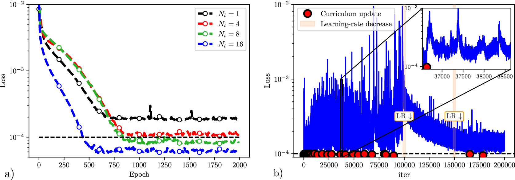
Figure 5. Long description
Panel a is a line graph with a logarithmic y-axis labeled Loss from 10 super minus 4 to 10 super minus 2 and an x-axis labeled Epoch from 0 to 2000. Four dashed lines with circular markers represent different latent space dimensions N sub ell. The blue line for N sub ell equals 16 shows the steepest initial descent, reaching a plateau near 6 times 10 super minus 5 by epoch 500. The green line for N sub ell equals 8 and red line for N sub ell equals 4 follow a similar path, plateauing near 8 times 10 super minus 5 and 10 super minus 4 respectively by epoch 1000. The black line for N sub ell equals 1 has the slowest descent, plateauing near 2 times 10 super minus 4. A horizontal black dashed line marks the 10 super minus 4 threshold.
Panel b is a line graph with a logarithmic y-axis labeled Loss and an x-axis labeled iter from 0 to 200,000. The data is a highly oscillatory blue line. Red circular markers along the bottom horizontal dashed line at 10 super minus 4 indicate curriculum updates. Two vertical shaded orange bands at approximately 100,000 and 150,000 iterations are labeled L R down arrow, indicating learning rate decreases. An inset in the top right corner provides a magnified view of the loss oscillations between 37,000 and 38,500 iterations, showing a curriculum update marker at the start of a spike.
Training NODEs on complex trajectories requires backpropagating through repeated evaluations of the neural network during time integration. Despite standard stabilizations, this integration depth often leads to exploding or vanishing gradients and reduced sensitivity (Chakraborty et al., Reference Chakraborty, Chung, Arcomano and Maulik2024). This difficulty is amplified when the target trajectories contain sharp transients, oscillatory segments, or bifurcating branches, all of which increase the sensitivity of the learned dynamics to small integration errors. Several training strategies have been designed to overcome the reduced sensitivity for neural ODEs, such as shooting methods (Turan and Jäschke, Reference Turan and Jäschke2021) to capture higher-frequency responses and the multistep penalty method (Chakraborty et al., Reference Chakraborty, Chung, Arcomano and Maulik2024) that splits trajectories into multiple, nonoverlapping time windows and includes an optimization loss term to penalize the window discontinuities. In the present work, vanilla training of the parameterized NODE model resulted in a loss function that failed to decay, and the learned solution trajectories artificially suppressed oscillatory components rather than capturing the true underlying dynamics. To address this, a curriculum learning strategy was introduced, which shares conceptual features with the multistep penalty method. In general, curriculum learning structures the optimization process such that training begins with simpler tasks and gradually progresses to more complex ones, thereby improving both convergence and generalization (Bucci et al., Reference Bucci, Semeraro, Allauzen, Chibbaro and Mathelin2023).
In the present application, task difficulty was defined by the temporal extent of the latent space trajectories. To clarify, all training samples of the input parameter space
$ \boldsymbol{\xi} $
 were available for learning, but only a restricted time interval of each trajectory. This contrasts the curriculum regularization approach (Krishnapriyan et al., Reference Krishnapriyan, Gholami, Zhe, Kirby and Mahoney2021) used in training of physics-informed neural networks that progressively samples different parts of the parameter space, leading to lower error rates. Curriculum learning was implemented as a staged optimization over progressively increasing trajectory lengths:


Thus, training initially considers only the earliest part of each trajectory, and the target time interval for learning is extended by
$ \Delta T $
 whenever the model reaches the prescribed loss tolerance. For NODE training, the encoded trajectories were linearly up-sampled from the original
$ {N}_t=20 $
whenever the model reaches the prescribed loss tolerance. For NODE training, the encoded trajectories were linearly up-sampled from the original
$ {N}_t=20 $
 postdeposition snapshots to
$ {N}_t^{\prime }=100 $
postdeposition snapshots to
$ {N}_t^{\prime }=100 $
 temporal samples. The full time series of the trajectory ensemble was divided into
$ {N}_L=50 $
temporal samples. The full time series of the trajectory ensemble was divided into
$ {N}_L=50 $
 folds, chosen as the maximum number that partitions the signal into integer-length segments, so that the curriculum increment was
$ \Delta T={N}_t^{\prime }/{N}_L $
folds, chosen as the maximum number that partitions the signal into integer-length segments, so that the curriculum increment was
$ \Delta T={N}_t^{\prime }/{N}_L $
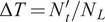 samples. The curriculum update tolerance was set to
$ \unicode{x025B} =1\times {10}^{-4} $
samples. The curriculum update tolerance was set to
$ \unicode{x025B} =1\times {10}^{-4} $
 , which by inspection corresponded to accurate capture of the characteristic curvature of the trajectories. Accordingly, the variation of the loss during NODE training is shown in Figure 5(b). The sharp increases in loss correspond to curriculum updates, where a new trajectory segment is exposed to the optimizer, while the subsequent decay indicates that the NODE progressively learns the newly introduced portion of the latent trajectory. This staged expansion of the learned trajectory segment is illustrated for representative latent components in Figure 6. As the training horizon is extended, the newly revealed portion of the trajectory initially exhibits larger error, after which optimization adjusts the latent dynamics to recover the correct direction of evolution in the added segment. In practice, these updates reduced the error in the newly introduced interval without noticeably degrading the already-learned earlier portion of the trajectory, although the curriculum update does not guarantee monotonic improvement on the previously exposed segment.
Representative case of latent space trajectories
$ {V}_{\mathrm{\ell}} $
 illustrating the curriculum learning process. Panels (a)–(d) display the advancing training window (gray band), highlighting the progressive learning of newly revealed trajectory segments as the time horizon extends. Dashed lines indicate the beginning prediction at the start of the update, while solid lines show the final learned trajectory.
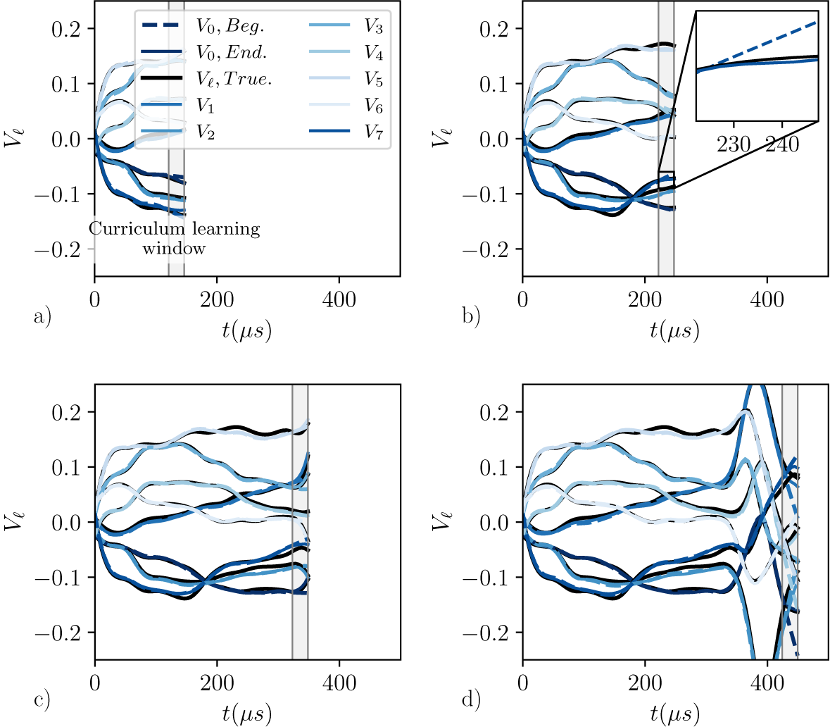
Figure 6. Long description
A four-panel line graph grid labeled a through d. Each panel shares the same axes: the x-axis is time t in mu s ranging from 0 to 500, and the y-axis is V sub ell ranging from -0.2 to 0.2.
* Panel a: A vertical gray band labeled Curriculum learning window is positioned early at approximately 120 to 150 mu s. Trajectories for V sub 0 through V sub 7 are plotted. Dashed lines represent the beginning prediction and solid lines represent the final learned trajectory. The lines are only visible up to the gray window.
* Panel b: The gray window has shifted right to approximately 220 to 250 mu s. An inset zoom-in shows the divergence between the dashed beginning prediction and the solid learned trajectory at the window’s edge.
* Panel c: The gray window has shifted further right to approximately 320 to 350 mu s. The trajectories are now learned and stable across a longer time horizon.
* Panel d: The gray window is near the end of the time scale at approximately 420 to 450 mu s. The trajectories show complex oscillating patterns that have been fully revealed and learned as the training window reached the final segment.
The legend in panel a identifies V sub 0 Beg. as a dashed dark blue line, V sub 0 End. as a solid dark blue line, and V sub ell True as a solid black line. Other trajectories V sub 1 through V sub 7 are shown in varying shades of blue.
The present training strategy uses a single NVIDIA Tesla P100 (16 GB) GPU for 24 hours to efficiently train the AE to spatially compress the data matrix
$ \mathcal{S} $
 into a learnable latent space, and subsequently, training the parameterized NODE takes 48 hours on a CPU. The key to making the present complex problem learnable in a realistic time frame was (i) a problem representation that retained the laser-spark kernel evolution dynamics, and combustion features, without being dominated by the multiscale complex spectrum of turbulence present in the numerical schlieren of a coflowing jet, and (ii) a curriculum learning strategy that allowed for complex trajectories with multiple modes and bifurcations to be learned.
4. Results
4.1. Latent space trajectories
To assess whether the trained model captures the essential dynamics of ignition, we first examine the latent space trajectories, i.e., the mapping of the CFD IR sequences from image space
$ {\mathbf{x}}^{(j)}\left({t}_i\right)\in {\unicode{x211D}}^{m\times n} $
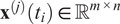 (
$ m,n=592\times 240 $
(
$ m,n=592\times 240 $
 ) by the AE into low-dimensional vectors
$ {\mathbf{V}}^{(j)}\left({t}_i\right)\in {\unicode{x211D}}^{N_{\mathrm{\ell}}} $
) by the AE into low-dimensional vectors
$ {\mathbf{V}}^{(j)}\left({t}_i\right)\in {\unicode{x211D}}^{N_{\mathrm{\ell}}} $
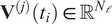 that is required to extract meaningful latent representations. At the time of spatial compression, the AE is not temporally aware and simply encodes possible combustor states; as a postprocessing step for analysis, we order the latent vectors in time
$ {\mathbf{V}}^{(j)}\left({t}_i\right) $
that is required to extract meaningful latent representations. At the time of spatial compression, the AE is not temporally aware and simply encodes possible combustor states; as a postprocessing step for analysis, we order the latent vectors in time
$ {\mathbf{V}}^{(j)}\left({t}_i\right) $
 for each trial with unique sample of
$ {\boldsymbol{\xi}}^{(j)} $
for each trial with unique sample of
$ {\boldsymbol{\xi}}^{(j)} $
 , yielding a family of trajectories. Figure 7 displays the latent components
$ {V}_{\mathrm{\ell}} $
, yielding a family of trajectories. Figure 7 displays the latent components
$ {V}_{\mathrm{\ell}} $
 as time series across the ensemble; after linear up-sampling, each trial forms a smooth curve. At early times, the coordinates capture the initial stages of laser deposition and kernel formation, with variance across cases small and tightly clustered. Subsequently, the trajectories reflect interaction with the co-flowing fuel–oxidizer shear layer, and finally, when
$ t\gtrsim 250\hskip0.1em \mu \mathrm{s} $
as time series across the ensemble; after linear up-sampling, each trial forms a smooth curve. At early times, the coordinates capture the initial stages of laser deposition and kernel formation, with variance across cases small and tightly clustered. Subsequently, the trajectories reflect interaction with the co-flowing fuel–oxidizer shear layer, and finally, when
$ t\gtrsim 250\hskip0.1em \mu \mathrm{s} $
 the bifurcating outcomes of either: (i) runaway combustion/ignition success or (ii) a dissipating kernel/ignition failure.
Temporal evolution of the eight latent-space components for the reacting rocket-combustor LES ensemble. Each curve corresponds to one ignition trial, with color indicating the informative input parameter
$ {\xi}_2=\beta ={R}_1/{R}_2 $
 . Each ignition trial contributes one trajectory
$ {\mathbf{V}}^{(j)}(t) $
. Each ignition trial contributes one trajectory
$ {\mathbf{V}}^{(j)}(t) $
 to the ensemble, and each subpanel shows a different component
$ {V}_{\mathrm{\ell}}^{(j)}(t) $
to the ensemble, and each subpanel shows a different component
$ {V}_{\mathrm{\ell}}^{(j)}(t) $
 of that latent vector.
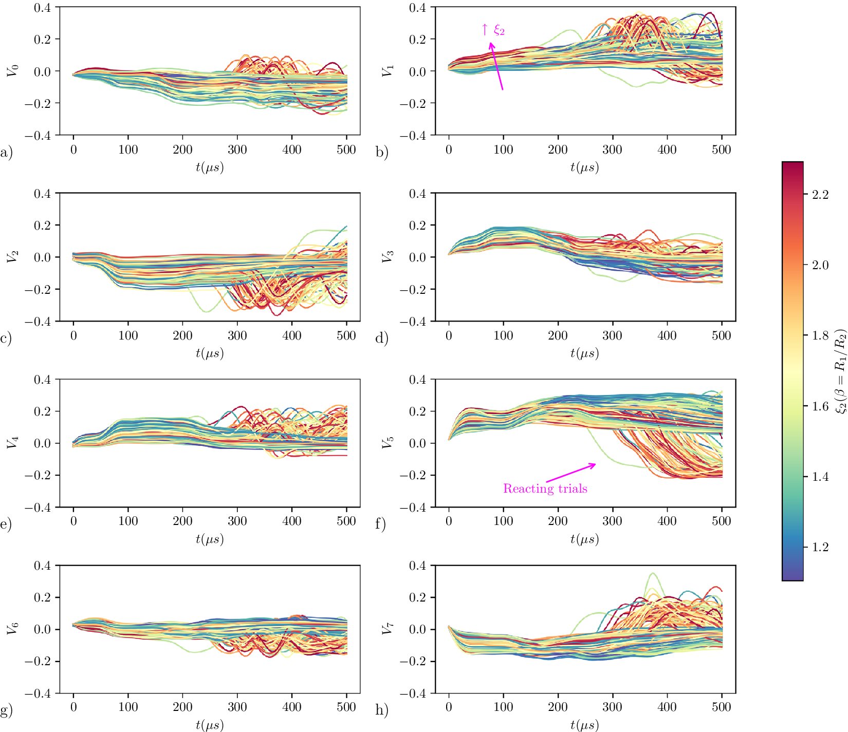
Figure 7. Long description
A multi-panel figure containing eight subplots arranged in two columns and four rows, labeled a through h. Each subplot shares an x-axis representing time t in microseconds from 0 to 500 and a y-axis representing the component value from negative 0.4 to 0.4.
* Subplot a, V sub 0: Curves remain near zero until 300 microseconds, where they begin to oscillate slightly.
* Subplot b, V sub 1: Curves show a gradual upward trend. A pink arrow points upward indicating increasing xi sub 2.
* Subplot c, V sub 2: Curves drop to negative 0.1 at 100 microseconds and show high-frequency oscillations after 300 microseconds.
* Subplot d, V sub 3: Curves rise to 0.1 and then diverge slightly after 200 microseconds.
* Subplot e, V sub 4: Curves rise to 0.1 and maintain a steady band with late-stage oscillations.
* Subplot f, V sub 5: Curves rise to 0.2. A pink arrow labeled Reacting trials points to a group of curves that drop sharply toward negative 0.2 after 300 microseconds.
* Subplot g, V sub 6: Curves remain near zero with minor oscillations starting at 250 microseconds.
* Subplot h, V sub 7: Curves initially dip to negative 0.1 before rising and oscillating after 300 microseconds.
A vertical color bar on the right indicates the parameter xi sub 2, which equals beta, which equals R sub 1 over R sub 2. The scale ranges from 1.2 in dark blue at the bottom to 2.2 in dark red at the top, with yellow representing the midpoint of 1.7.
The latent space thus provides a reduced representation that preserves essential dynamics in compact form. For reference, in previous work on steady aerodynamics, systematic analysis of latent components yielded physical insight into the individual role of inviscid and viscous contributions (Saetta et al., Reference Saetta, Tognaccini and Iaccarino2024a, Reference Saetta, Tognaccini and Iaccarinob). This was achieved by sequentially training and conditioning the latent space to separate physical processes. In the present application, the latent space could therefore be interrogated by systematically deactivating components of the latent space vector
$ \mathbf{V} $
 to uncover what physics each component
$ {V}_{\mathrm{\ell}} $
to uncover what physics each component
$ {V}_{\mathrm{\ell}} $
 is capturing, analogous to modal analysis; however, analysis of the physical processes captured by each latent space variable is beyond the present scope of work. Instead, the present focus is to develop a predictive generative model for rocket ignition. In this setting, as the input vector
$ \boldsymbol{\xi} $
is capturing, analogous to modal analysis; however, analysis of the physical processes captured by each latent space variable is beyond the present scope of work. Instead, the present focus is to develop a predictive generative model for rocket ignition. In this setting, as the input vector
$ \boldsymbol{\xi} $
 is sampled for the input conditions for a particular ignition trial, the key requirement for the model is to predict how the corresponding latent state evolves in time, i.e., we require a structured mapping
$ \boldsymbol{\xi} \mapsto \mathbf{V}\left(t;\boldsymbol{\xi} \right) $
is sampled for the input conditions for a particular ignition trial, the key requirement for the model is to predict how the corresponding latent state evolves in time, i.e., we require a structured mapping
$ \boldsymbol{\xi} \mapsto \mathbf{V}\left(t;\boldsymbol{\xi} \right) $
 , where
$ \mathbf{V}\left(t;\boldsymbol{\xi} \right) $
, where
$ \mathbf{V}\left(t;\boldsymbol{\xi} \right) $
 denotes the latent trajectory generated over the ignition sequence for that choice of input parameters. Figure 7 illustrates this structured mapping by coloring each trajectory with an informative input parameter
$ {\xi}_2=\beta ={R}_1/{R}_2 $
denotes the latent trajectory generated over the ignition sequence for that choice of input parameters. Figure 7 illustrates this structured mapping by coloring each trajectory with an informative input parameter
$ {\xi}_2=\beta ={R}_1/{R}_2 $
 (laser lobe asymmetry, see Table A1, Appendix A), highlighting the correlation between input variability and latent evolution.
The early stages (
$ t<200\;\mu s $
 ) of the laser spark dynamics are only weakly modulated by the presence of the coflowing shear layer and instead are governed by the baroclinic torque, which varies with laser input parameters (Wang et al., Reference Wang, Buchta and Freund2020). The corresponding representation in latent space should therefore be a smooth response to the input parameter vector
$ \boldsymbol{\xi} $
) of the laser spark dynamics are only weakly modulated by the presence of the coflowing shear layer and instead are governed by the baroclinic torque, which varies with laser input parameters (Wang et al., Reference Wang, Buchta and Freund2020). The corresponding representation in latent space should therefore be a smooth response to the input parameter vector
$ \boldsymbol{\xi} $
 . Accordingly, Figure 7(b) is annotated at
$ t=100\mu s $
. Accordingly, Figure 7(b) is annotated at
$ t=100\mu s $
 to highlight that increasing values of
$ {\xi}_2 $
to highlight that increasing values of
$ {\xi}_2 $
 on average correspond to an increase in
$ {V}_1 $
on average correspond to an increase in
$ {V}_1 $
 . Further, a statistically clear mapping from
$ {\xi}_2 $
. Further, a statistically clear mapping from
$ {\xi}_2 $
 to the latent space of
$ {V}_3 $
to the latent space of
$ {V}_3 $
 in Figure 7(d) is also observed. Note, postprocessing or sensitivity analysis could be applied to inspect the degree of structured mapping from input parameter to latent space for every component of
$ \boldsymbol{\xi} $
in Figure 7(d) is also observed. Note, postprocessing or sensitivity analysis could be applied to inspect the degree of structured mapping from input parameter to latent space for every component of
$ \boldsymbol{\xi} $
 , and when
$ {\xi}_4={l}_{axial} $
, and when
$ {\xi}_4={l}_{axial} $
 (laser axial length) was chosen, clearer and higher degree of correlation was observed in early-time kernel reflecting the importance to the early laser deposition physics. Concerning early-time kernel dynamics, preliminary work on nonreacting sparks (Zahtila et al., Reference Zahtila, Saetta, Brouzet, Cutforth, Rossinelli and Iaccarino2024) showed that a high amount of variance occurred very early, with thereafter a period of relatively constant values, underscoring the importance of fast kernel dynamics.
Focusing on dynamics after the ignition time scale
$ t\gtrsim 250\hskip0.1em \mu \mathrm{s} $
 , consistent trajectories emerge: successful ignitions oscillate and for some latent space components branch off while ignition failures persist with stable values and small variation. Oscillations appear in several components of the latent space
$ \mathbf{V} $
, consistent trajectories emerge: successful ignitions oscillate and for some latent space components branch off while ignition failures persist with stable values and small variation. Oscillations appear in several components of the latent space
$ \mathbf{V} $
 for igniting cases, but the degree of oscillation in each component varies; for instance, in Figure 7(a), the range of the oscillation values does not depart significantly from the nonignited cases, unlike in Figure 7(h), where positive values of
$ {V}_7 $
for igniting cases, but the degree of oscillation in each component varies; for instance, in Figure 7(a), the range of the oscillation values does not depart significantly from the nonignited cases, unlike in Figure 7(h), where positive values of
$ {V}_7 $
 are observed exclusively during the oscillatory phase. Strong separation in the latent space between successful and failed ignition is most visible in the clearly separated bifurcation branches of component
$ {V}_5 $
are observed exclusively during the oscillatory phase. Strong separation in the latent space between successful and failed ignition is most visible in the clearly separated bifurcation branches of component
$ {V}_5 $
 , visualized in Figure 7(f). Given the clear role of component
$ {V}_5 $
, visualized in Figure 7(f). Given the clear role of component
$ {V}_5 $
 in separating cases by ignition fate in the latent space, we project the latent trajectories onto two-dimensional component planes to provide interpretable slices of the manifold, in which clustering, variance, and separation are more readily discerned, as shown in Figure 8. Although some projection planes do not reveal strong separation by ignition fate and are less informative, in Figure 8(c), a very clear region of the latent space path is followed in the
$ {V}_5-{V}_2 $
in separating cases by ignition fate in the latent space, we project the latent trajectories onto two-dimensional component planes to provide interpretable slices of the manifold, in which clustering, variance, and separation are more readily discerned, as shown in Figure 8. Although some projection planes do not reveal strong separation by ignition fate and are less informative, in Figure 8(c), a very clear region of the latent space path is followed in the
$ {V}_5-{V}_2 $
 plane for ignition success. Clusters of the terminating ignition trial trajectory points in the
$ {V}_5-{V}_2 $
plane for ignition success. Clusters of the terminating ignition trial trajectory points in the
$ {V}_5-{V}_2 $
 plane reflect the bistable ignition bifurcation and the evolution path through latent space.
Latent space projections of
$ {V}_5 $
 against all other latent variables for the reacting sparks simulation ensemble, colored by the laser lobe asymmetry input parameter
$ {\xi}_2=\beta ={R}_1/{R}_2 $
against all other latent variables for the reacting sparks simulation ensemble, colored by the laser lobe asymmetry input parameter
$ {\xi}_2=\beta ={R}_1/{R}_2 $
 . Each trajectory begins at a green hollow circle and terminates at a red hollow circle, illustrating consistent trajectories in the low-dimensional manifold and separation of igniting from nonigniting cases.
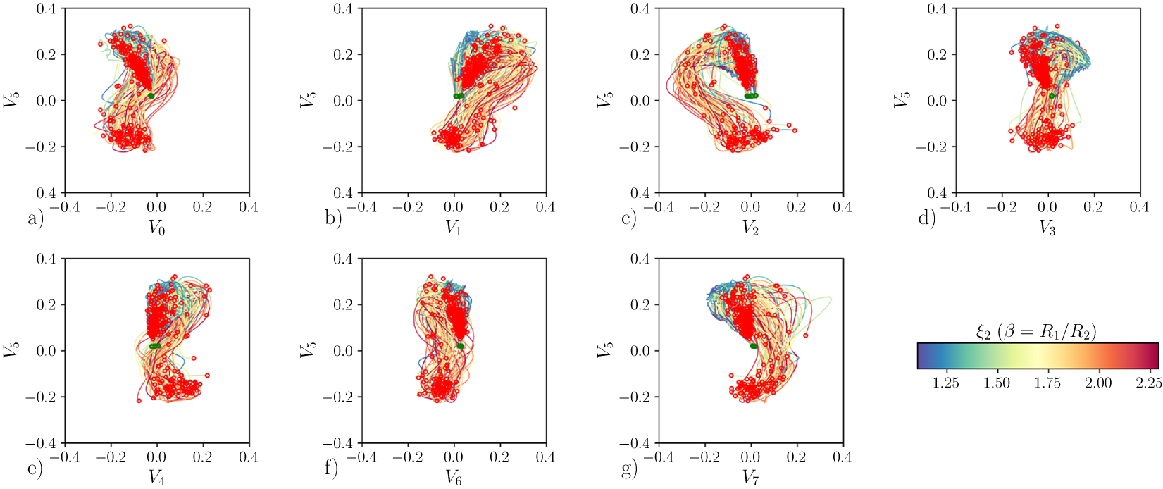
Figure 8. Long description
A multi-panel figure containing seven attribute space diagrams labeled a through g and a color scale bar.
Each plot shares a common Y axis labeled V sub 5 ranging from negative 0.4 to 0.4. The X axes represent different latent variables V sub n, also ranging from negative 0.4 to 0.4.
* Panel a: V sub 5 versus V sub 0. Data shows a dense cluster of red hollow circles in the upper-left and lower-left quadrants connected by curved trajectories.
* Panel b: V sub 5 versus V sub 1. Trajectories move from a lower-left cluster to an upper-right cluster.
* Panel c: V sub 5 versus V sub 2. Shows a wide C-shaped distribution of trajectories.
* Panel d: V sub 5 versus V sub 3. Features a vertical hourglass-shaped distribution centered around X equals 0.
* Panel e: V sub 5 versus V sub 4. Shows a slightly tilted vertical distribution.
* Panel f: V sub 5 versus V sub 6. Displays a dense vertical column of trajectories.
* Panel g: V sub 5 versus V sub 7. Shows trajectories curving from the bottom-center toward the top-left.
In all panels, trajectories are colored according to the parameter xi sub 2, which equals beta, which equals R sub 1 forward slash R sub 2. Green hollow circles mark the start of trajectories and red hollow circles mark the termination points.
A horizontal color scale bar at the bottom right maps xi sub 2 values from 1.25 in dark blue, through green and yellow at 1.75, to dark red at 2.25.
Previous surrogate-modeling efforts combining AEs with latent dynamics, including NODE-based approaches (Lazzara et al., Reference Lazzara, Chevalier, Lapeyre, Teste, Iliadis, Papaleonidas, Angelov and Jayne2023), have typically addressed systems with a simpler spectrum such as the viscous 1D Burgers equation with an expectation that they admit a coherent latent representation. In contrast, the present rocket–combustor system is a multiphysics problem involving turbulence, heat release, and bistable ignition outcomes, so it cannot be assumed a priori that the AE will produce a latent space with smooth and physically meaningful organization. We therefore first examined the latent space structure to determine whether nearby points corresponded to physically similar states and whether variations in the latent trajectories remained systematically related to the governing input parameters
$ \boldsymbol{\xi} $
 and the associated ignition dynamics. This provided evidence that the encoded dynamics evolved on a coherent low-dimensional manifold whose organization retained dependence on
$ \boldsymbol{\xi} $
and the associated ignition dynamics. This provided evidence that the encoded dynamics evolved on a coherent low-dimensional manifold whose organization retained dependence on
$ \boldsymbol{\xi} $
 , and hence that the latent trajectories were amenable to learning. Overall, Figures 7 and 8 together demonstrate that (i) ignition trials embed as smooth latent manifold trajectories; (ii) variance across trajectories reflects sensitivity to variability of input parameters; and (iii) bifurcations encode ignition fate, particularly through the role of
$ {V}_5 $
, and hence that the latent trajectories were amenable to learning. Overall, Figures 7 and 8 together demonstrate that (i) ignition trials embed as smooth latent manifold trajectories; (ii) variance across trajectories reflects sensitivity to variability of input parameters; and (iii) bifurcations encode ignition fate, particularly through the role of
$ {V}_5 $
 . Taken together, these observations confirm that the learned manifold provides a physically meaningful description of the ignition process, in which early-time clustering, mid-time shear-layer interaction, and ignition-time bifurcations are all preserved. This representation therefore establishes a suitable foundation for NODE-based temporal modeling, as the latent coordinates capture both common trajectories and their bistable outcomes in a consistent reduced-order form.
4.2. Performance of the DnAE
Following the accurate encoding of key physical processes captured by the separation and clustering of the AE latent space, we now investigate two components of the DnAE framework: (i) the predictive modeling capability of the NODE to temporally integrate an ODE within the reduced latent space, and (ii) the fidelity of the resulting spatiotemporal sequence output from the decoder. The only required inputs to yield a prediction from the trained DnAE are specification of the input parameter vector
$ \boldsymbol{\xi} $
 and an initial latent state
$ {\mathbf{V}}_0 $
and an initial latent state
$ {\mathbf{V}}_0 $
 , which together define a unique ignition trial scenario. In this section, we first evaluate the NODE-integrated latent trajectories
$ \hat{\mathbf{V}}(t) $
, which together define a unique ignition trial scenario. In this section, we first evaluate the NODE-integrated latent trajectories
$ \hat{\mathbf{V}}(t) $
 relative to their target trajectories
$ \mathbf{V}(t) $
relative to their target trajectories
$ \mathbf{V}(t) $
 in the latent space, and subsequently, focus on the decoder output
$ \hat{\mathbf{x}}(t)=d\left[\hat{\mathbf{V}}(t)\right] $
in the latent space, and subsequently, focus on the decoder output
$ \hat{\mathbf{x}}(t)=d\left[\hat{\mathbf{V}}(t)\right] $
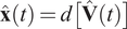 to assess the framework’s ability to generate physically realistic reconstructions and to predict ignition success across a diverse range of initial conditions.
Figure 9 presents the individual components of the AE latent space with overlaid trajectories predicted from the NODE with representative cases shown corresponding to the 5th, 50th, and 95th percentiles of prediction error, illustrating strong, median, and weak accuracy, respectively. The trajectories are disjointly arranged into training and validation runs. For the training runs, it becomes clear that the curriculum-learning trained neural ODE is able to reconstruct the full diversity of latent space trajectories and trajectory variance introduced by variation in the input parameter vector
$ \boldsymbol{\xi} $
 . This represents a considerable extension to the complexity of features learned by neural ODE trajectories when compared with previous work on springs (Garsdal et al., Reference Garsdal, Søgaard and Sørensen2022), or exponentially growing, saturating trajectories (Owoyele and Pal, Reference Owoyele and Pal2022). Based on the training trajectories, the NODE accurately captures the AE latent space dynamics during the early stages of kernel evolution and reproduces the oscillatory behavior characteristic of reacting cases.
Training (left columns) and validation (right columns) latent trajectories generated by the neural ODE, compared with the target latent-space trajectories. Representative cases are shown for the 5th, 50th, and 95th percentiles of RMSE, corresponding to strong, median, and weak prediction accuracy, respectively. The shaded region indicates the ensemble distribution of the full set of latent-space trajectories.
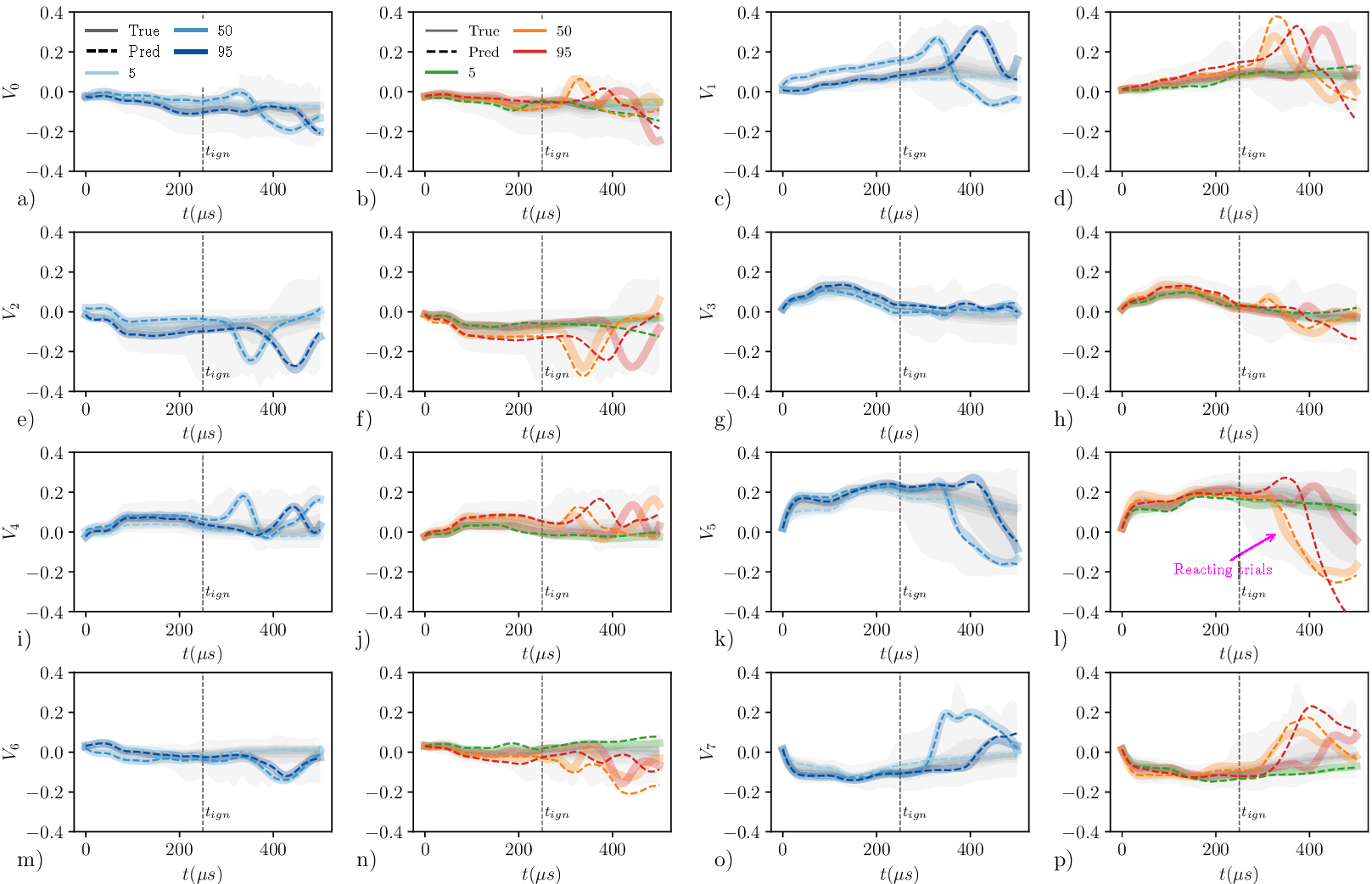
Figure 9. Long description
A grid of 16 line graphs labeled a through p. Each graph shares a common x-axis representing time t in micro-seconds (mu s) from 0 to 500, and a y-axis representing latent variable values from negative 0.4 to 0.4. A vertical dashed line at approximately 250 mu s marks t sub ign.
* The first and second columns (panels a, b, e, f, i, j, m, n) show training data for variables V sub 0, V sub 2, V sub 4, and V sub 6.
* The third and fourth columns (panels c, d, g, h, k, l, o, p) show validation data for variables V sub 1, V sub 3, V sub 5, and V sub 7.
* Solid lines represent True values, while dashed lines represent Predicted values.
* Colors indicate accuracy percentiles: light blue or green for the 5th percentile (strong), medium blue or orange for the 50th percentile (median), and dark blue or red for the 95th percentile (weak).
* A light gray shaded region in the background of each plot represents the ensemble distribution.
* In the training panels, the predicted dashed lines closely follow the solid true lines, showing high fidelity.
* In the validation panels, particularly for the 95th percentile (red and dark blue lines), the predicted trajectories deviate significantly from the true values after the t sub ign mark, often exhibiting oscillatory behavior or sharp declines.
* Panel l includes a pink arrow pointing to a diverging trajectory labeled Reacting trials.
For the validation cases, the NODE-evolved latent trajectories
$ \hat{\mathbf{V}}(t) $
 broadly followed the true dynamics
$ \mathbf{V}(t) $
broadly followed the true dynamics
$ \mathbf{V}(t) $
 during the early stages of kernel evolution and up until the ignition time scale but began to diverge once the reacting phase commenced. This behavior is consistent with the chaotic nature of the reacting system, where predictive accuracy typically degrades as trajectories evolve. To assess this quantitatively, we divided each trajectory into four equal-duration time intervals, denoted Q1–Q4 from earliest to latest. For each quarter, we computed both the Frechet distance (Sochopoulos et al., Reference Sochopoulos, Gienger and Vijayakumar2024) and
$ {L}_2 $
during the early stages of kernel evolution and up until the ignition time scale but began to diverge once the reacting phase commenced. This behavior is consistent with the chaotic nature of the reacting system, where predictive accuracy typically degrades as trajectories evolve. To assess this quantitatively, we divided each trajectory into four equal-duration time intervals, denoted Q1–Q4 from earliest to latest. For each quarter, we computed both the Frechet distance (Sochopoulos et al., Reference Sochopoulos, Gienger and Vijayakumar2024) and
$ {L}_2 $
 norm between the predicted and true latent coordinates, and both metrics showed strong agreement in trends. As shown in Table 1, errors were relatively low across the first two segments (Q1–Q2), but increased substantially in later times (Q3–Q4), reflecting divergence on a chaotic attractor which arises from turbulent combustion. Despite this divergence, the NODE reliably captured key qualitative features—such as the collapse of trajectories for nonigniting cases and persistent oscillations for successful ignition. To clarify, the NODE is expected to track the target latent trajectories
$ \mathbf{V}(t) $
norm between the predicted and true latent coordinates, and both metrics showed strong agreement in trends. As shown in Table 1, errors were relatively low across the first two segments (Q1–Q2), but increased substantially in later times (Q3–Q4), reflecting divergence on a chaotic attractor which arises from turbulent combustion. Despite this divergence, the NODE reliably captured key qualitative features—such as the collapse of trajectories for nonigniting cases and persistent oscillations for successful ignition. To clarify, the NODE is expected to track the target latent trajectories
$ \mathbf{V}(t) $
 during the early-time kernel dynamics and to correctly trace the shear-layer interactions that bifurcate toward ignition success or failure. Thereafter, the NODE is only expected to capture the qualitative features of either combustion success or failure rather than one-to-one matching of the turbulent state. The remedy to long-time divergence would require state assimilation methods (e.g., EnKF; Özalp et al., Reference Özalp, Nóvoa and Magri2025), which offer dramatically improved late-time accuracy; however, they require repeated observations and impose strict system sampling constraints, which on the time scales of rocket ignition are out of the question. The present framework, by contrast, requires no additional system observations beyond the initial condition.
Error metric in NODE-predicted latent space trajectories across four temporal quarters (Q1–Q4) across training and validation data split

Table 1. Long description
The table is divided into two main columns: Train and Validation, each subdivided into four temporal quarters: Q 1, Q 2, Q 3, and Q 4.
Row 1: Fréchet distance.
- Train values: Q 1 is 0.009, Q 2 is 0.013, Q 3 is 0.018, and Q 4 is 0.035.
- Validation values: Q 1 is 0.075, Q 2 is 0.100, Q 3 is 0.190, and Q 4 is 0.289.
Row 2: L 2 Norm.
- Train values: Q 1 is 0.002, Q 2 is 0.003, Q 3 is 0.005, and Q 4 is 0.007.
- Validation values: Q 1 is 0.021, Q 2 is 0.029, Q 3 is 0.048, and Q 4 is 0.080.
Both metrics show a progressive increase in error from Q 1 to Q 4, with significantly higher error rates in the Validation set compared to the Train set.
Note. Results reflect transition from early-time kernel dynamics to late-time divergence in the chaotic reacting phase.
At the conclusion of the neural ODE integration, the resultant latent trajectory is passed through the decoder
$ d\left(\cdot \right) $
 to generate the reconstructed spatiotemporal sequence
$ \hat{\mathbf{x}}\left({t}_i\right)=d\left[\hat{\mathbf{V}}\left({t}_i\right)\right] $
to generate the reconstructed spatiotemporal sequence
$ \hat{\mathbf{x}}\left({t}_i\right)=d\left[\hat{\mathbf{V}}\left({t}_i\right)\right] $
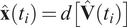 at the sampled times which for the available dataset can be directly compared one-to-one with the corresponding IR post-processed CFD sequence
$ {\mathbf{x}}^{(j)}(t) $
at the sampled times which for the available dataset can be directly compared one-to-one with the corresponding IR post-processed CFD sequence
$ {\mathbf{x}}^{(j)}(t) $
 . For automated ignition classification, each reconstructed field
$ {\hat{\mathbf{x}}}^{(j)}(t) $
. For automated ignition classification, each reconstructed field
$ {\hat{\mathbf{x}}}^{(j)}(t) $
 is segmented into iso-temperature contours, and ignition success is determined based on the area enclosed by a
$ {T}_0 $
is segmented into iso-temperature contours, and ignition success is determined based on the area enclosed by a
$ {T}_0 $
 -isotherm,

where
$ {T}_0 $
 is the user-prescribed threshold temperature,
$ \boldsymbol{s} $
is the user-prescribed threshold temperature,
$ \boldsymbol{s} $
 denotes position in the projected two-dimensional image plane, and
$ {\Omega}_{T_0}^{(j)}(t) $
denotes position in the projected two-dimensional image plane, and
$ {\Omega}_{T_0}^{(j)}(t) $
 denotes the spatially evolving region bounded by the corresponding temperature isotherm. Ignition success is subsequently recorded when
$ {A}_{T_0}^{(j)}(t) $
denotes the spatially evolving region bounded by the corresponding temperature isotherm. Ignition success is subsequently recorded when
$ {A}_{T_0}^{(j)}(t) $
 exhibits sustained growth over the postdeposition sequence, with
$ {T}_0=1000\hskip0.22em \mathrm{K} $
exhibits sustained growth over the postdeposition sequence, with
$ {T}_0=1000\hskip0.22em \mathrm{K} $
 in the present study. This criterion corresponds to sustained flame expansion and was found to be insensitive to variations in the chosen threshold temperature.
The DnAE performance in ignition success prediction is therefore summarized by the confusion matrices presented in Figure 10, with
$ 10\% $
 of the original data held out for validation. The training confusion matrix in Figure 10(a) shows near-perfect classification performance, with a single ignition trial incorrectly labeled. For the ignition (positive) class, the precision and recall were
$ 0.99 $
of the original data held out for validation. The training confusion matrix in Figure 10(a) shows near-perfect classification performance, with a single ignition trial incorrectly labeled. For the ignition (positive) class, the precision and recall were
$ 0.99 $
 and
$ 1.00 $
and
$ 1.00 $
 . In general, classification difficulty is predicated on class imbalance and for the present rocket ignition reliability task, imbalance is quantified through class entropy,
$ H({p}_{\mathrm{ign}})=-{p}_{\mathrm{ign}}{\log}_2{p}_{\mathrm{ign}}-(1-{p}_{\mathrm{ign}}){\log}_2(1-{p}_{\mathrm{ign}})=0.85\mathrm{bits} $
. In general, classification difficulty is predicated on class imbalance and for the present rocket ignition reliability task, imbalance is quantified through class entropy,
$ H({p}_{\mathrm{ign}})=-{p}_{\mathrm{ign}}{\log}_2{p}_{\mathrm{ign}}-(1-{p}_{\mathrm{ign}}){\log}_2(1-{p}_{\mathrm{ign}})=0.85\mathrm{bits} $
 , where for class entropy the maximum uncertainty, i.e.,
$ p=0.5 $
, where for class entropy the maximum uncertainty, i.e.,
$ p=0.5 $
 results in 1.0 bits, therefore the present classification challenge is significant. The validation confusion matrix shown in Figure 10(b) indicates reduced but still reasonable predictive performance, with an overall ignition classification accuracy of
$ 80\% $
results in 1.0 bits, therefore the present classification challenge is significant. The validation confusion matrix shown in Figure 10(b) indicates reduced but still reasonable predictive performance, with an overall ignition classification accuracy of
$ 80\% $
 , with ignition prediction precision and recall both
$ 0.70 $
, with ignition prediction precision and recall both
$ 0.70 $
 indicating balanced false-positive and false-negative rates on this validation split. Rather than stemming from systematic class bias, misclassifications are attributed to the divergence of the predicted latent state from the ground truth, causing the trajectory to cross into a region of the latent space that evolves toward the incorrect ignition fate—a characteristic limitation when modeling chaotic dynamical systems (Solera-Rico et al., Reference Solera-Rico, Vila, Gómez-López, Wang, Almashjary, Dawson and Vinuesa2024). The validation performance on unseen cases indicated by the confusion matrix in Figure 10(b) is satisfactory although misclassifications suggest that broader sampling of the input space would improve generalization. The near-perfect training performance, together with the lower validation accuracy, indicates a gap between in-sample fit and out-of-sample generalization. This suggests that, given the present dataset size, coverage of the parameter space, and problem complexity, the model would benefit from broader sampling, but this is characteristic of the data scenario in machine learning for combustion, where CFD simulations are costly.
Confusion matrices for the binary classification of ignition outcomes. (a) Training set results, with near-perfect separation between failure and success cases. (b) Validation set performance.
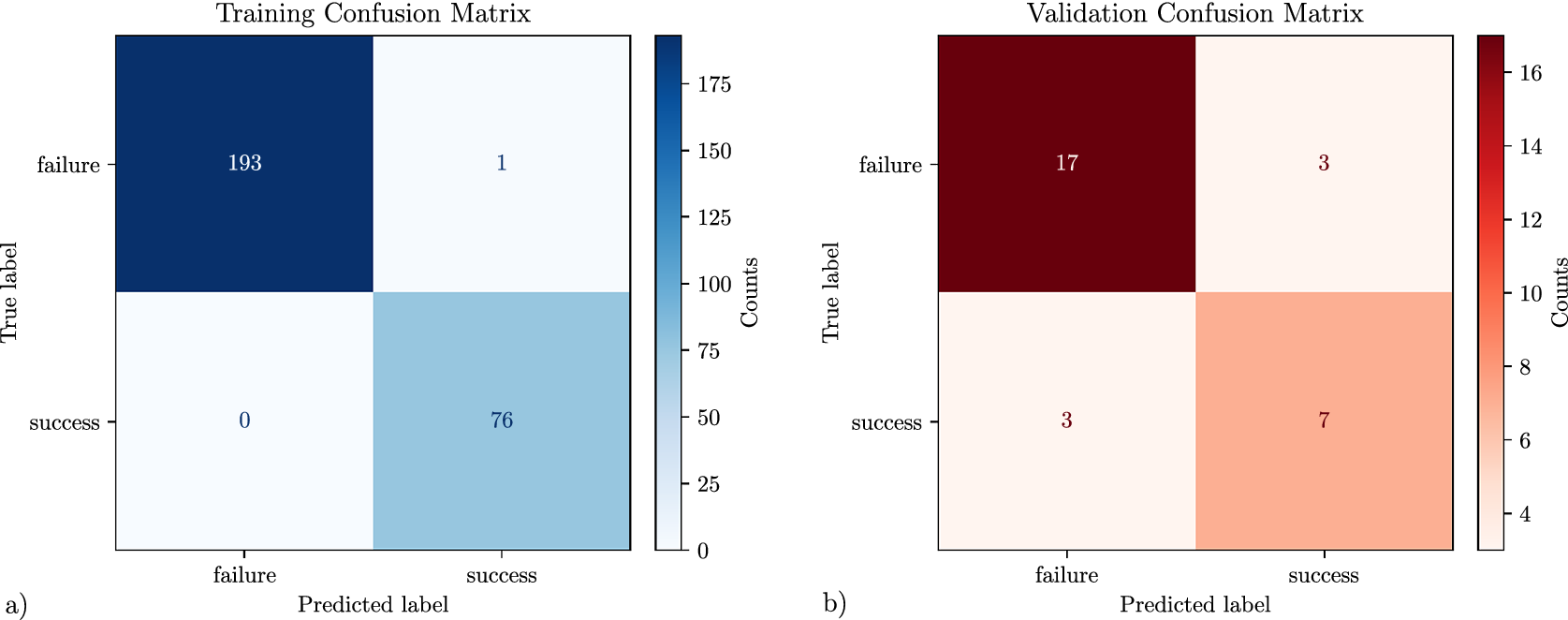
Figure 10. Long description
Two side-by-side confusion matrices labeled a and b. Both matrices use True label on the vertical axis and Predicted label on the horizontal axis with categories failure and success.
Panel a, Training Confusion Matrix. A blue color scale indicates counts from 0 to 175.
* Top-left (True failure, Predicted failure): 193, dark blue.
* Top-right (True failure, Predicted success): 1, white.
* Bottom-left (True success, Predicted failure): 0, white.
* Bottom-right (True success, Predicted success): 76, light blue.
Panel b, Validation Confusion Matrix. A red color scale indicates counts from 4 to 16.
* Top-left (True failure, Predicted failure): 17, dark red.
* Top-right (True failure, Predicted success): 3, white.
* Bottom-left (True success, Predicted failure): 3, white.
* Bottom-right (True success, Predicted success): 7, light orange.
Visualizations of the reconstructed DnAE spatiotemporal sequence,
$ \hat{\mathbf{x}}(t)=d\left[\hat{\mathbf{V}}(t)\right] $
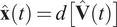 , are shown in Figure 11 and compared with the one-to-one counterpart CFD IR imaging. A subset of cases was selected to illustrate ignition success and failure within the training dataset, as shown in Figure 11(a,b). These results show that the latent space of the AE is sufficiently smooth and continuous that time-evolved latent states remain physically accurate. Additionally, representative outcomes for each category in the validation confusion matrix are presented in Figure 11(c–f) to demonstrate both correctly and incorrectly classified ignition events. Starting with the training reconstruction of an igniting sequence shown in Figure 11(a), the DnAE correctly identifies the ignition onset timing relative to the reference CFD IR sequence. The reconstructed flame exhibits a comparable spatial extent to the CFD IR field, though with visibly reduced fine-scale structure. This loss of small-scale content is consistent with prior findings that accurate compression of the full energy spectrum of turbulent flow fields requires a very large latent dimension, typically orders of magnitude larger than present, to preserve small-scale information and avoid the masking of reconstruction errors (Vinograd and Di Leoni, Reference Vinograd and Di Leoni2025). Figure 11(c,f) illustrate correctly classified spatiotemporal sequences in which both the flame growth and ignition onset are well reproduced. Across the dataset, the DnAE typically achieves ignition onset predictions within an error of
$ \Delta t\approx 25\hskip0.1em \mu \mathrm{s} $
, are shown in Figure 11 and compared with the one-to-one counterpart CFD IR imaging. A subset of cases was selected to illustrate ignition success and failure within the training dataset, as shown in Figure 11(a,b). These results show that the latent space of the AE is sufficiently smooth and continuous that time-evolved latent states remain physically accurate. Additionally, representative outcomes for each category in the validation confusion matrix are presented in Figure 11(c–f) to demonstrate both correctly and incorrectly classified ignition events. Starting with the training reconstruction of an igniting sequence shown in Figure 11(a), the DnAE correctly identifies the ignition onset timing relative to the reference CFD IR sequence. The reconstructed flame exhibits a comparable spatial extent to the CFD IR field, though with visibly reduced fine-scale structure. This loss of small-scale content is consistent with prior findings that accurate compression of the full energy spectrum of turbulent flow fields requires a very large latent dimension, typically orders of magnitude larger than present, to preserve small-scale information and avoid the masking of reconstruction errors (Vinograd and Di Leoni, Reference Vinograd and Di Leoni2025). Figure 11(c,f) illustrate correctly classified spatiotemporal sequences in which both the flame growth and ignition onset are well reproduced. Across the dataset, the DnAE typically achieves ignition onset predictions within an error of
$ \Delta t\approx 25\hskip0.1em \mu \mathrm{s} $
 of the reference. Misclassifications, shown in Figure 11(d,e), nonetheless retain physically coherent structures, indicating that the latent representation remains dynamically consistent even when classification errors occur.
One-to-one comparison between DnAE-reconstructed IR sequences and the corresponding CFD IR reference sequences for representative ignition outcomes. Panels (a, b) show training cases for ignition success and ignition failure, respectively. Panels (c–f) show validation cases corresponding to the confusion-matrix outcomes in Figure 10: (c) true negative, (d) false positive, (e) false negative, and (f) true positive.
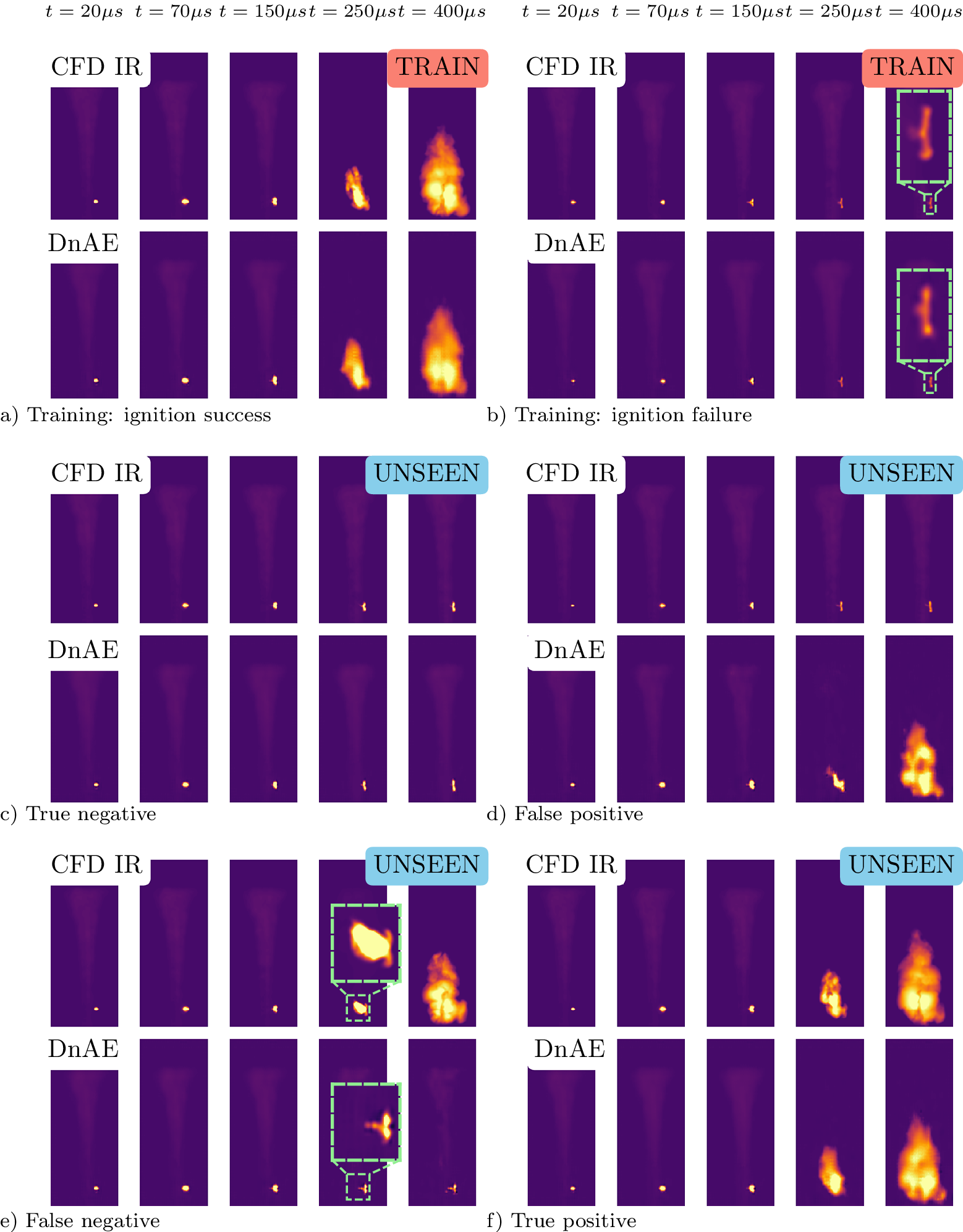
Figure 11. Long description
The multi-panel visualization consists of six panels labeled a through f. Each panel contains two rows of five vertical heatmaps representing time steps at t = 20, 70, 150, 250, and 400 microseconds. The top row in each panel is labeled C F D I R and the bottom row is labeled D n A E.
* Panel a (Training: ignition success): Both rows show a small bright kernel at 20 microseconds that grows into a large, bright plume by 400 microseconds. The D n A E reconstruction closely matches the C F D I R reference.
* Panel b (Training: ignition failure): Both rows show a small kernel that remains small and eventually dissipates. A green dashed box highlights the similarity in the final frame.
* Panel c (True negative): Both rows show a small kernel that fails to ignite, remaining as a tiny dot through 400 microseconds.
* Panel d (False positive): The C F D I R row shows ignition failure with a small dot, but the D n A E row incorrectly reconstructs a large, bright ignition plume at 400 microseconds.
* Panel e (False negative): The C F D I R row shows a successful ignition plume at 400 microseconds, while the D n A E row incorrectly shows a dissipated, small kernel. Green dashed boxes highlight the discrepancy at 250 microseconds.
* Panel f (True positive): Both rows show the progression from a small kernel to a large, bright ignition plume at 400 microseconds, indicating a successful reconstruction of an unseen case.
Panels a and b are marked with a red TRAIN tag, while panels c through f are marked with a blue UNSEEN tag.
The present performance of the DnAE highlights that accurate integration across bistable time horizons remains inherently difficult; however, the model performance is satisfactory given the highdegree of variability in ignition process arising from the aleatoric uncertainty associated with instantaneous turbulence. Using the law of total variance, with
$ {\xi}_6 $
 (laser lag time) treated as the aleatoric uncertainty accounting for the instantaneous structure of turbulence and the remaining inputs treated as epistemic, the binary ignition fate was decomposed as
$ \mathrm{Var}(Ign)={\unicode{x1D53C}}_{{\boldsymbol{\xi}}_{\mathrm{epi}}}\left[\mathrm{Var}\left( Ign|{\boldsymbol{\xi}}_{\mathrm{epi}}\right)\right]+{\mathrm{Var}}_{{\boldsymbol{\xi}}_{\mathrm{epi}}}\left(\unicode{x1D53C}\left[ Ign|{\boldsymbol{\xi}}_{\mathrm{epi}}\right]\right) $
(laser lag time) treated as the aleatoric uncertainty accounting for the instantaneous structure of turbulence and the remaining inputs treated as epistemic, the binary ignition fate was decomposed as
$ \mathrm{Var}(Ign)={\unicode{x1D53C}}_{{\boldsymbol{\xi}}_{\mathrm{epi}}}\left[\mathrm{Var}\left( Ign|{\boldsymbol{\xi}}_{\mathrm{epi}}\right)\right]+{\mathrm{Var}}_{{\boldsymbol{\xi}}_{\mathrm{epi}}}\left(\unicode{x1D53C}\left[ Ign|{\boldsymbol{\xi}}_{\mathrm{epi}}\right]\right) $
 . This yielded run-to-run ignition fate variance fractions for the aleatoric and epistemic contributions of
$ 0.39 $
. This yielded run-to-run ignition fate variance fractions for the aleatoric and epistemic contributions of
$ 0.39 $
 and
$ 0.61 $
and
$ 0.61 $
 , respectively. A preceding physics-based study on the role of the instantaneous turbulent structure in ignition dynamics found that small changes in local flow features can drive bifurcating ignition outcomes (Wang et al., Reference Wang, Di Renzo, Iaccarino, Wang and Urzay2024). With the physically consistent reconstructions observed in Figures 11(d,e), we suggest that each trial is a physically realizable ignition trajectory, reflecting the stochasticity encoded within the latent space due to the variance introduced by the structure of instantaneous turbulence. The observed variability largely reflects the underlying randomness and sensitivity of the system rather than systematic model error.
4.3. Large-scale sampling and generative features
The motivation for employing a generative model in UQ arises from the prohibitive cost of repeated CFD evaluations. Even in low-fidelity settings, a single deployment typically requires wall-clock times on the order of hours (Zahtila et al., Reference Zahtila, Passiatore and Iaccarino2023; Lee et al., Reference Lee, Chan, Zahtila, Lu, Iaccarino and Ooi2025) on modern heterogeneous architectures. Consequently, efficient characterization of system responses across the input space becomes computationally intractable, particularly in the presence of high-dimensional input parameter spaces. The solution of the forward CFD problem with machine learning has received significant attention (Vlachas et al., Reference Vlachas, Pathak, Hunt, Sapsis, Girvan, Ott and Koumoutsakos2020) and is a current development topic for appropriate generalization and baselines (McGreivy and Hakim, Reference McGreivy and Hakim2024). In this work, we leverage the rapid deployment capabilities of the DnAE framework to propagate input uncertainties and approximate ignition response at a scale of
$ {N}_{\mathrm{MC}}=\mathcal{O}\left({10}^6\right) $
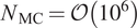 realizations, and we accept as a tradeoff a reduction in physical fidelity that would arise from performing scale-resolving LES computations. Obtaining
$ {N}_{\mathrm{MC}}=\mathcal{O}\left({10}^6\right) $
realizations, and we accept as a tradeoff a reduction in physical fidelity that would arise from performing scale-resolving LES computations. Obtaining
$ {N}_{\mathrm{MC}}=\mathcal{O}\left({10}^6\right) $
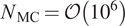 samples of the input space would be infeasible through classical numerical simulation but using the present framework is deployable on a single workstation. This accessibility does not preclude scaling; the framework could be transitioned to high-performance clusters where significantly higher dimensional latent spaces could be utilized, followed by decoding and analysis of the resulting spatiotemporal quantities.
The additional requirement, compared to the preceding section featuring one-to-one corresponding CFD IR model output, is the specification of an initial condition in the latent space, obtained here via radial basis function interpolation of the sampled initial conditions as a function of the input parameter vector
$ \boldsymbol{\xi} $
 , i.e.,
$ {\mathbf{V}}_0\left(\boldsymbol{\xi} \right)=\mathrm{RBF}\left(\boldsymbol{\xi}; {\left\{{\boldsymbol{\xi}}^{(k)},{\mathbf{V}}_0^{(k)}\right\}}_{k=1}^{N_c}\right) $
, i.e.,
$ {\mathbf{V}}_0\left(\boldsymbol{\xi} \right)=\mathrm{RBF}\left(\boldsymbol{\xi}; {\left\{{\boldsymbol{\xi}}^{(k)},{\mathbf{V}}_0^{(k)}\right\}}_{k=1}^{N_c}\right) $
 , where
$ {\boldsymbol{\xi}}^{(k)} $
, where
$ {\boldsymbol{\xi}}^{(k)} $
 denotes the
$ k $
denotes the
$ k $
 th sampled parameter vector and
$ {\mathbf{V}}_0^{(k)} $
th sampled parameter vector and
$ {\mathbf{V}}_0^{(k)} $
 the corresponding initial condition from the LES ensemble set, an approximation error
$ \unicode{x025B} $
the corresponding initial condition from the LES ensemble set, an approximation error
$ \unicode{x025B} $
 is introduced to the initial latent space state but we expect this error to be small because the initial image in the sequence is sampled just prior to laser spark deposition and therefore reflects only the aleatoric uncertainty in the uncontrollable instantaneous jet structure; moreover, there is little variance in the magnitude of the latent space vector at this initial stage. New samples of
$ \boldsymbol{\xi} $
is introduced to the initial latent space state but we expect this error to be small because the initial image in the sequence is sampled just prior to laser spark deposition and therefore reflects only the aleatoric uncertainty in the uncontrollable instantaneous jet structure; moreover, there is little variance in the magnitude of the latent space vector at this initial stage. New samples of
$ \boldsymbol{\xi} $
 are therefore drawn in accordance with their probability distributions documented in Appendix A Table A1. To ensure the generated samples remain within the geometric support of the training data, they would ideally reside within the convex hull of the uncertainty space spanned by
$ \boldsymbol{\xi} $
are therefore drawn in accordance with their probability distributions documented in Appendix A Table A1. To ensure the generated samples remain within the geometric support of the training data, they would ideally reside within the convex hull of the uncertainty space spanned by
$ \boldsymbol{\xi} $
 and would therefore be interpolative. However, because this space is high-dimensional and explicit convex-hull computation scales poorly with dimensionality, a simpler criterion is adopted: generative samples are instead constrained to lie within the component-wise bounds (minimum and maximum) of each uncertainty component
$ {\xi}_i $
and would therefore be interpolative. However, because this space is high-dimensional and explicit convex-hull computation scales poorly with dimensionality, a simpler criterion is adopted: generative samples are instead constrained to lie within the component-wise bounds (minimum and maximum) of each uncertainty component
$ {\xi}_i $
 as determined from the training ensemble.
A restricted sample of the resulting large-scale generated set of trajectories is shown in Figure 12. For all latent space components
$ {V}_{\mathrm{\ell}} $
 , the variance during early-time intervals remains consistent with that of the training trajectories, indicating that the generative model follows the latent manifold dynamics. However, in the flame growth regime, oscillatory trajectories extend beyond the variance of the CFD IR set, but this is consistent with the behavior expected from more dense sampling from a chaotic turbulent attractor. Trajectories are classified into igniting and nonigniting on the basis of separation in component
$ {V}_5 $
, the variance during early-time intervals remains consistent with that of the training trajectories, indicating that the generative model follows the latent manifold dynamics. However, in the flame growth regime, oscillatory trajectories extend beyond the variance of the CFD IR set, but this is consistent with the behavior expected from more dense sampling from a chaotic turbulent attractor. Trajectories are classified into igniting and nonigniting on the basis of separation in component
$ {V}_5 $
 , where departure from the steady solution branch into negative
$ {V}_5 $
, where departure from the steady solution branch into negative
$ {V}_5 $
 indicates ignition success, as noted in Section 4.1, introducing separation in latent space as a classifier. This is taken as an alternative to the previous contour-area growth criterion from the reconstructed spatiotemporal sequence
$ \hat{\mathbf{x}}(t)=d\left[\hat{\mathbf{V}}(t)\right] $
indicates ignition success, as noted in Section 4.1, introducing separation in latent space as a classifier. This is taken as an alternative to the previous contour-area growth criterion from the reconstructed spatiotemporal sequence
$ \hat{\mathbf{x}}(t)=d\left[\hat{\mathbf{V}}(t)\right] $
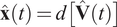 as the decoder introduces a significant additional cost required for the segmentation process. Although beyond the scope of the present focus, a high-accuracy spatiotemporal surrogate provides a pathway to examine detailed combustion behaviors, including flame anchoring, directly via the NODE evolution and quantitative comparison with reference physics (Brouzet et al., Reference Brouzet, Rossinelli, Zahtila, Voci, Strelau, Warner, Gejji, Slabaugh and Iaccarino2026).
Generative latent-space trajectory predictions for unseen cases output by the DnAE, classified as either igniting or nonigniting; a reduced subset is shown. Each panel corresponds to one component of the latent vector
$ \hat{\mathbf{V}}(t) $
 . For reference, the range of trajectories on the low-dimensional manifold extracted from compressed CFD IR data is shaded in the background, where
$ {\hat{\mathbf{V}}}_f(t) $
. For reference, the range of trajectories on the low-dimensional manifold extracted from compressed CFD IR data is shaded in the background, where
$ {\hat{\mathbf{V}}}_f(t) $
 denotes predicted latent trajectories associated with ignition failure and
$ {\hat{\mathbf{V}}}_s(t) $
denotes predicted latent trajectories associated with ignition failure and
$ {\hat{\mathbf{V}}}_s(t) $
 denotes those associated with ignition success.
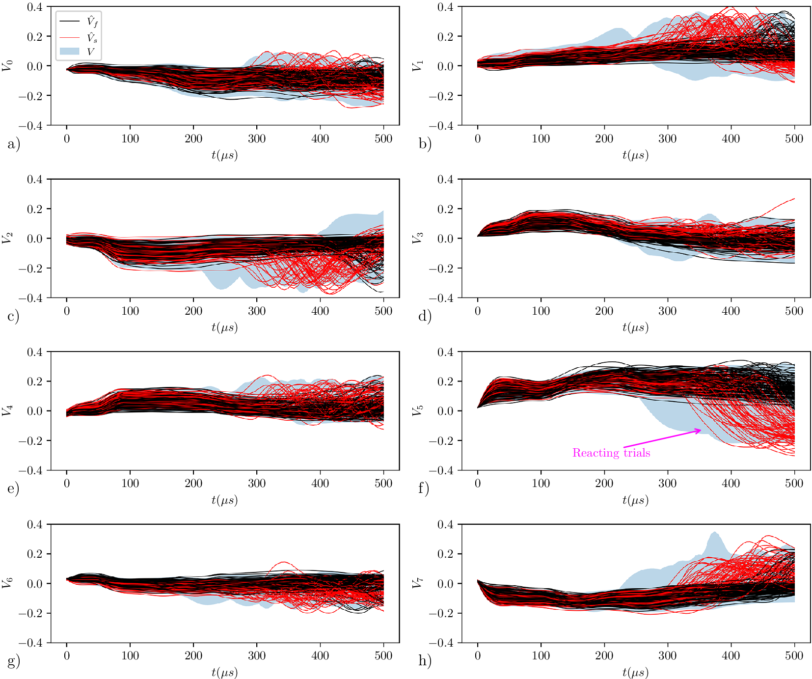
Figure 12. Long description
The figure consists of eight panels arranged in two columns and four rows, labeled a through h. Each panel shares a common x-axis representing time t in microseconds from 0 to 500 and a y-axis representing a latent vector component V sub n from negative 0.4 to 0.4.
In every panel, three data layers are present. First, a light blue shaded region in the background represents the range of trajectories from compressed C F D I R data. Second, black lines represent predicted latent trajectories associated with ignition failure, V hat sub f. Third, red lines represent predicted latent trajectories associated with ignition success, V hat sub s.
* Panel a, V sub 0. Trajectories remain relatively flat near 0 until 300 microseconds, where red lines begin to oscillate within the blue shaded region.
* Panel b, V sub 1. Trajectories show a slight upward trend. Red lines exhibit higher variance and peaks between 300 and 400 microseconds.
* Panel c, V sub 2. Lines show a downward dip around 100 microseconds. Red lines diverge significantly into a lower blue shaded lobe after 300 microseconds.
* Panel d, V sub 3. Trajectories rise to 0.1 by 100 microseconds then gradually decline. Red lines show higher density near 0 after 300 microseconds.
* Panel e, V sub 4. Similar to panel d, but red lines show a distinct upward burst between 300 and 400 microseconds.
* Panel f, V sub 5. Trajectories rise and plateau. A magenta arrow points to a cluster of red lines diverging downward after 350 microseconds, labeled Reacting trials.
* Panel g, V sub 6. Trajectories are stable near 0. Red lines show minor oscillations in the latter half of the timeline.
* Panel h, V sub 7. Trajectories dip slightly below 0. Red lines show a sharp upward trend into a blue shaded peak between 350 and 500 microseconds.
Given the present reliability context of rocket ignition success, a key outcome of this framework is the ability to estimate ignition probability landscapes over the input parameter space at a resolution unattainable with CFD alone. By drawing
$ {N}_{\mathrm{MC}}=\mathcal{O}\left({10}^6\right) $
 Monte Carlo samples, we construct joint probability distributions of the statistically important controllable laser operating parameters identified in Section 2.1, where high K–L divergence between their igniting and nonigniting marginal probability distributions reveals how ignition likelihood varies. As the number of samples dramatically increases from that afforded by the CFD IR data stream alone, the estimated probability fields converge to stable contours. Crucially, decision boundaries corresponding to ignition success probabilities of
$ \mathit{\Pr}= $
Monte Carlo samples, we construct joint probability distributions of the statistically important controllable laser operating parameters identified in Section 2.1, where high K–L divergence between their igniting and nonigniting marginal probability distributions reveals how ignition likelihood varies. As the number of samples dramatically increases from that afforded by the CFD IR data stream alone, the estimated probability fields converge to stable contours. Crucially, decision boundaries corresponding to ignition success probabilities of
$ \mathit{\Pr}= $
 0.5, 0.75, and 0.9 can be identified directly within these landscapes, as shown in Figure 13. We find in the converged Figure 13(d) that a combination of high laser energy (
$ {\xi}_5 $
0.5, 0.75, and 0.9 can be identified directly within these landscapes, as shown in Figure 13. We find in the converged Figure 13(d) that a combination of high laser energy (
$ {\xi}_5 $
 ), deposited over an increased axial length (
$ {\xi}_4 $
), deposited over an increased axial length (
$ {\xi}_4 $
 ), and with deposition lobe asymmetry (
$ {\xi}_2 $
), and with deposition lobe asymmetry (
$ {\xi}_2 $
 ) leads to high likelihood of ignition success. These provide laser design thresholds and recommended operating conditions. This capability transforms the surrogate model from a mere predictor of individual trajectories into a quantitative tool for uncertainty-informed decision making, where reliability can be assessed in terms of probability contours rather than binary outcomes.
Joint ignition probability distributions, estimated via Monte Carlo sampling of the NODE latent space trajectories, as a function of the input parameter pairs (
$ \beta, E $
 ) (top row) and (
$ \beta, {l}_{axial} $
) (top row) and (
$ \beta, {l}_{axial} $
 ) (bottom row), obtained using (a) 300 samples, (b) 200,000 samples, (c) 500,000 samples, and (d) 1,000,000 samples. Additionally marked are decision boundaries for
$ \mathit{\Pr}(ign)=\mathit{0.5,0.75,0.9} $
) (bottom row), obtained using (a) 300 samples, (b) 200,000 samples, (c) 500,000 samples, and (d) 1,000,000 samples. Additionally marked are decision boundaries for
$ \mathit{\Pr}(ign)=\mathit{0.5,0.75,0.9} $
 .
.
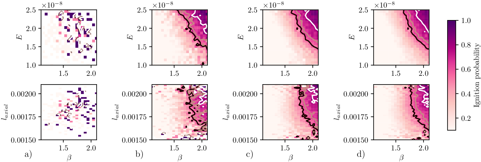
Figure 13. Long description
The multi-panel layout consists of two rows labeled a through d from left to right.
In the top row, the y-axis is E times 10 super minus 8 and the x-axis is beta. In the bottom row, the y-axis is l sub axial and the x-axis is beta.
Panel a uses 300 samples and shows a sparse, noisy distribution of dark purple pixels in the upper right quadrant.
Panel b uses 200,000 samples, showing a smoother gradient where probability increases toward the top-right corner. Three contour lines represent decision boundaries for probability equals 0.5, 0.75, and 0.9.
Panel c uses 500,000 samples and Panel d uses 1,000,000 samples. Both show increasingly refined and smooth probability gradients compared to panel b, with the high-probability dark purple region concentrated in the upper right.
In all panels, the transition from light pink to dark purple indicates an increasing ignition probability. A vertical color bar on the far right provides the scale from 0.0 (white) to 1.0 (dark purple). The decision boundaries appear as black, grey, and white lines moving from the lower-left toward the upper-right of the high-density regions.
5. Conclusions
In this paper, we present dynamical autoencoders (DnAE) that extend the generative cAE paradigm previously employed for steady-state aerodynamics. This surrogate model first compresses CFD-based IR field representations into a low-dimensional latent manifold
$ \mathbf{V} $
 through an AE, yielding a learnable mapping between the input parameter vector
$ \boldsymbol{\xi} $
through an AE, yielding a learnable mapping between the input parameter vector
$ \boldsymbol{\xi} $
 and the latent manifold
$ \mathbf{V} $
and the latent manifold
$ \mathbf{V} $
 . The dynamic extension is achieved through parameterized neural ODEs in the latent space to forecast complex ignition trajectories in the context of laser-ignited rocket combustors. The DnAE approach dramatically reduced computational cost compared to a forward pass of a scale-resolving simulation and remained capable of emulating the spatiotemporal evolution of the path-integrated IR fields that lead to critical ignition events.
A methodology devised for learning the complex trajectories that individual trials follow in the latent manifold was essential for capturing the bistable ignition fate of the system. We demonstrated that a curriculum learning strategy, which progressively extends the neural ODE forecast to longer trajectory horizons, was necessary to stabilize the learning process because standard training methods failed. Inspection of the latent space suggested a clear region of the latent space manifold where igniting cases (specifically in
$ {V}_5 $
 ) had been attracted, clearly separating successful ignition and failure branches. The decoder component
$ d\left(\cdot \right) $
) had been attracted, clearly separating successful ignition and failure branches. The decoder component
$ d\left(\cdot \right) $
 further allowed for the reconstruction of physically realistic thermal imaging sequences
$ \hat{\mathbf{x}}(t) $
further allowed for the reconstruction of physically realistic thermal imaging sequences
$ \hat{\mathbf{x}}(t) $
 , enabling one-to-one comparison against integrated quantities derived from reference large eddy simulation data and verifying that the model captures the correct mechanisms of kernel growth.
The utility of the developed surrogate model is a shift from sparse samples in the input parameter space to converged joint probability landscapes of ignition success in response to the operating laser input parameters. The DnAE framework facilitated the generation of
$ {N}_{\mathrm{MC}}={10}^6 $
 ignition trials, giving statistical power for these findings. The outcome is the demarcation of complex decision boundaries within the laser operating parameter space
$ \boldsymbol{\xi} $
ignition trials, giving statistical power for these findings. The outcome is the demarcation of complex decision boundaries within the laser operating parameter space
$ \boldsymbol{\xi} $
 . By quantifying the probability of ignition success
$ \mathit{\Pr}\left(\mathrm{ign}\right) $
. By quantifying the probability of ignition success
$ \mathit{\Pr}\left(\mathrm{ign}\right) $
 with high statistical confidence, this work provides a robust tool for uncertainty-informed design.
Acknowledgments
The authors also extend their gratitude to Dr. Gianluca Geraci for helpful discussions pertaining to this work.
Author contribution
Conceptualization: T.Z., G.I., M.C., and D.R. Methodology: T.Z., E.S., M.C., D.B., and D.R. Software: T.Z., M.C., and D. B. Data curation: T.Z., E.S., M.C., D.B., and D.R. Investigation: T.Z. Validation: T.Z. and E.S. Visualization: T.Z. and D.R. Writing – original draft: T.Z. Writing – review & editing: all authors. Supervision: D.R. and G.I. All authors approved the final submitted draft.
Competing interests
The authors declare none.
Data availability statement
The datasets used to generate the findings of this study are available from Zenodo (Zahtila, Reference Zahtila2026) at https://doi.org/10.5281/zenodo.18091817. The code that illustrates training and prediction for latent-space forecasting is available in the L-NeuralODE GitHub repository (Zahtila, Reference Zahtila2026) at https://github.com/tzahtila1/L-NeuralODE.
Funding statement
The authors acknowledge financial support from the US Department of Energy’s National Nuclear Security Administration via the Stanford PSAAP-III Center for the prediction of laser ignition of a rocket combustor (DE-NA0003968).
Ethical standards
The research meets all ethical guidelines, including adherence to the legal requirements of the study country.
A. Uncertainty parameters characterization
The input parameters for each ignition trial are samples from system variabilities in Table A1.
Summary of the
$ 15 $
 uncertain input parameters,
$ {\xi}_i $
uncertain input parameters,
$ {\xi}_i $
 , used in the ignition-trial uncertainty quantification, together with their physical descriptions, provenance, and assigned probability distributions
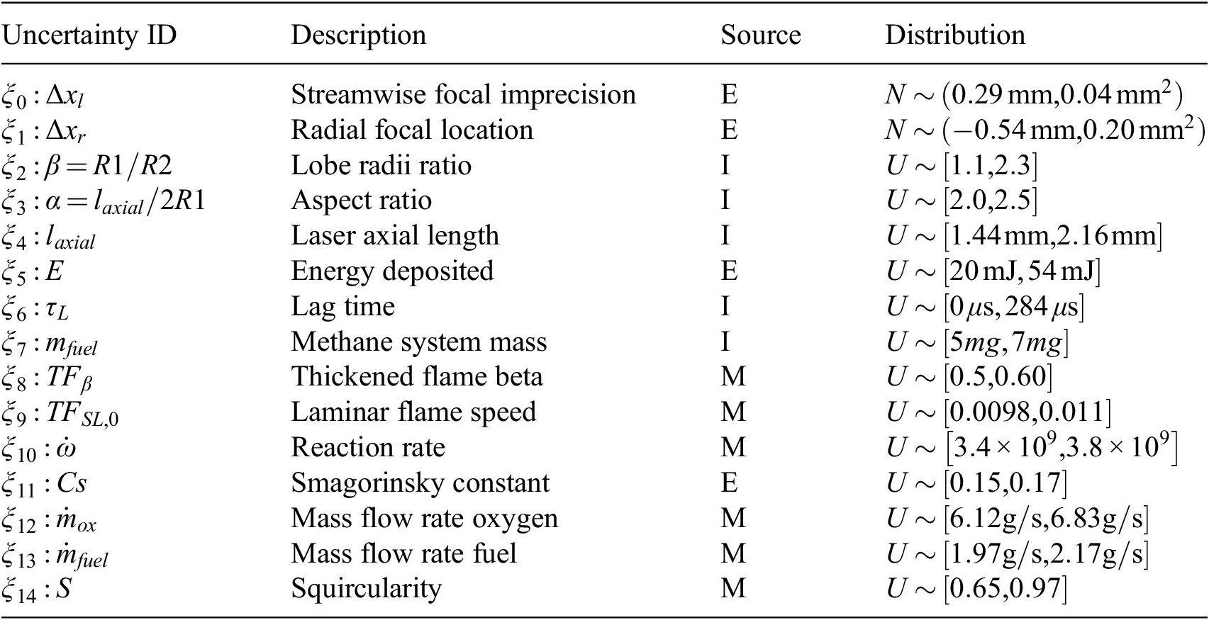
Table A1. Long description
The table consists of four columns: Uncertainty I D, Description, Source, and Distribution. It lists 15 parameters labeled xi sub 0 through xi sub 14.
* xi sub 0: Streamwise focal imprecision. Source E. Distribution N is approximately (0.29 mm, 0.04 mm squared).
* xi sub 1: Radial focal location. Source E. Distribution N is approximately (-0.54 mm, 0.20 mm squared).
* xi sub 2: Lobe radii ratio (beta = R 1 / R 2). Source I. Distribution U is approximately [1.1, 2.3].
* xi sub 3: Aspect ratio (alpha = l sub axial / 2 R 1). Source I. Distribution U is approximately [2.0, 2.5].
* xi sub 4: Laser axial length (l sub axial). Source I. Distribution U is approximately [1.44 mm, 2.16 mm].
* xi sub 5: Energy deposited (E). Source E. Distribution U is approximately [20 mJ, 54 mJ].
* xi sub 6: Lag time (tau sub L). Source I. Distribution U is approximately [0 microseconds, 284 microseconds].
* xi sub 7: Methane system mass (m sub fuel). Source I. Distribution U is approximately [5 mg, 7 mg].
* xi sub 8: Thickened flame beta (T F sub beta). Source M. Distribution U is approximately [0.5, 0.60].
* xi sub 9: Laminar flame speed (T F sub S L, 0). Source M. Distribution U is approximately [0.0098, 0.011].
* xi sub 10: Reaction rate (omega dot). Source M. Distribution U is approximately [3.4 times 10 super 9, 3.8 times 10 super 9].
* xi sub 11: Smagorinsky constant (C s). Source E. Distribution U is approximately [0.15, 0.17].
* xi sub 12: Mass flow rate oxygen (m dot sub ox). Source M. Distribution U is approximately [6.12 g/s, 6.83 g/s].
* xi sub 13: Mass flow rate fuel (m dot sub fuel). Source M. Distribution U is approximately [1.97 g/s, 2.17 g/s].
* xi sub 14: Squircularity (S). Source M. Distribution U is approximately [0.65, 0.97].
A footnote explains that U denotes a uniform distribution and N denotes a normal distribution with mean mu and variance sigma squared. Sources are E (experimentally measured), I (inferred), or M (model-form assumption).
These correspond to laser operating variabilities (
$ {\xi}_0-{\xi}_5 $
 ), aleatoric uncertainty associated with instantaneous turbulence realization (
$ {\xi}_6 $
), aleatoric uncertainty associated with instantaneous turbulence realization (
$ {\xi}_6 $
 ), fuel load (
$ {\xi}_7 $
), fuel load (
$ {\xi}_7 $
 ), LES model form uncertainties (
$ {\xi}_8-{\xi}_{11} $
), LES model form uncertainties (
$ {\xi}_8-{\xi}_{11} $
 ), operating conditions of the rocket (
$ {\xi}_{12}-{\xi}_{13} $
), operating conditions of the rocket (
$ {\xi}_{12}-{\xi}_{13} $
 ), and modeled geometry (
$ {\xi}_{14} $
), and modeled geometry (
$ {\xi}_{14} $
 ). The parameters are marked in the source column to indicate whether the statistical distribution was obtained by fit to the experimental data collected in the companion gas-phase model rocket combustor campaign (Strelau et al., Reference Strelau, Frederick, Winter, Senior, Gejji and Slabaugh2024), inferred from companion simulations (Brouzet et al., Reference Brouzet, Zahtila, Rossinelli, Voci, Iaccarino, Passiatore, Strelau, Gejji and Slabaugh2025), or model form assumptions.


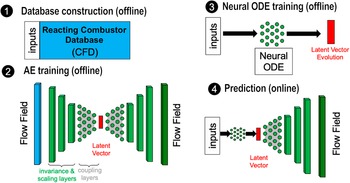
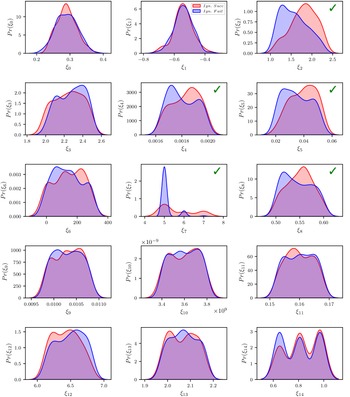


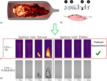
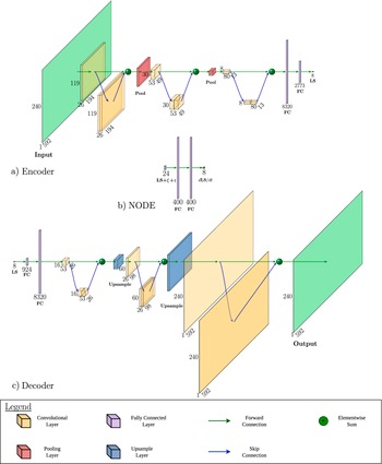


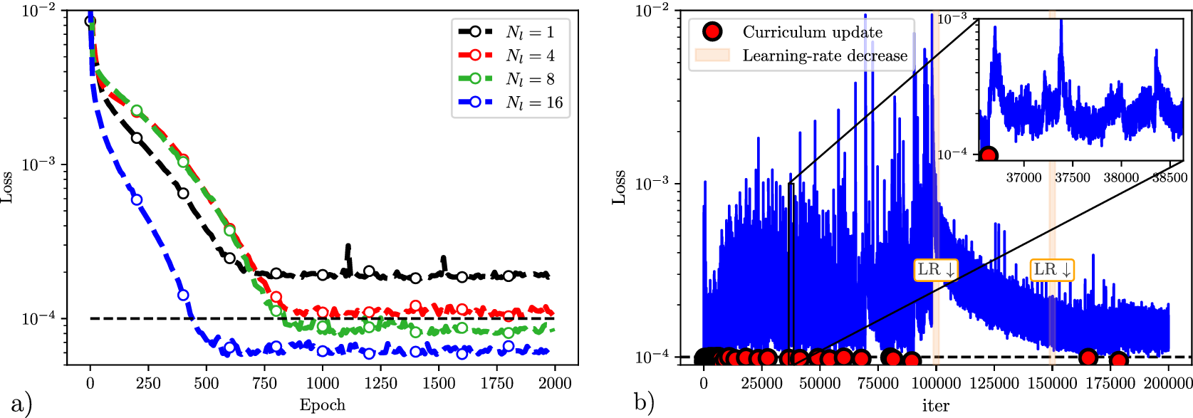


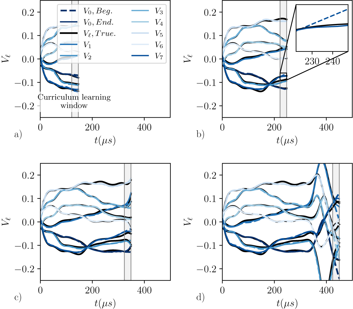

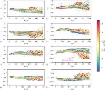


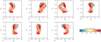


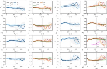

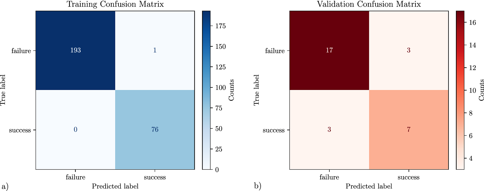
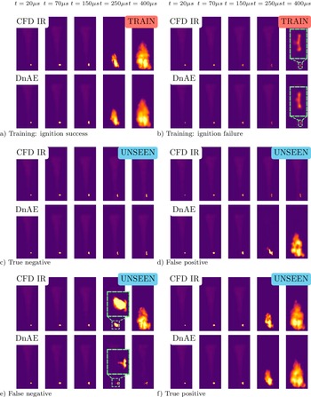
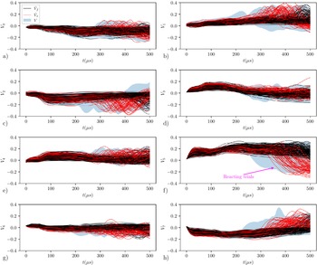


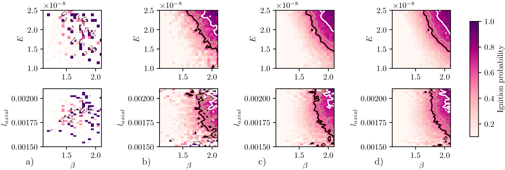


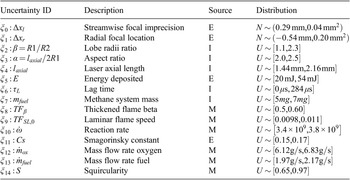


 Open access


Comments
No Comments have been published for this article.