


Nomenclature
- AAE
-
atypical air environment
- AAL
-
above aerodrome level
- ADS-B
-
Automated Dependent Surveillance – Broadcast
- AGL
-
above ground level
- AMSL
-
above mean sea level
- ANSP
-
air navigation service provider
- ARP
-
aerodrome reference point
- ATZ
-
aerodrome traffic zone
- BTP
-
British Transport Police
- BVLOS
-
beyond visual line of sight
- CAA
-
Civil Aviation Authority
- CAT
-
commercial air transport
- DAA
-
detect and avoid
- DEM
-
digital elevation model
- EC
-
electronic conspicuity
- ECMWF
-
European Centre for Medium-Range Weather Forecasts
- ERA5
-
ECMWF Reanalysis v5
- FLARM
-
Flight Alarm
- FRZ
-
flight restriction zone
- GA
-
General Aviation
- GNSS
-
Global Navigation Satellite System
- HLS
-
helicopter landing site
- HPC
-
High Performance Computing
- IFR
-
instrument flight rules
- ISA
-
International Standard Atmosphere
- JARUS
-
Joint Authorities for Rulemaking on Unmanned Systems
- MAC
-
mid-air collision
- METAR
-
Meteorological Aerodrome Report
- NAA
-
National Aviation Authority
- NOTAM
-
Notice To Airmen
- NR
-
Network Rail
- ORS
-
Official Record Series
- OS
-
Ordinance Survey
- PSR
-
primary surveillance radar
- RLOS
-
radio line of sight
- ROI
-
region of interest
- RP
-
remote pilot
- RPZ
-
runway protection zone
- SERA
-
Standardised European Rules of the Air
- SORA
-
Specific Operations Risk Assessment
- SRTM
-
Shuttle Radar Topography Mission
- SSR
-
secondary surveillance radar
- SWAP
-
size, weight and power
- TCAS
-
Traffic Collision Avoidance System
- TLS
-
target level of safety
- UA
-
uncrewed aircraft
- UK
-
United Kingdom
- VFR
-
visual flight rules
- VLOS
-
visual line of sight
Greek symbol
- $\alpha $
-
element along extended centreline
-
$\beta $
-
element normal to
$\alpha $
-
${{{\hat \Lambda }}_{{\textrm{enc}}}}$
-
normalised cumulative encounter rate
-
${\lambda _{{\textrm{MAC}}}}$
-
mid-air collision rate
-
${{{\Phi }}_P}$
-
geopotential


1.0 INTRODUCTION
The widespread introduction of uncrewed aircraft (UA) into civilian airspace rightly requires a high degree of confidence that a collision with a crewed aircraft is extremely improbable. For the vast majority of current operations within the United Kingdom (UK), this is achieved by enforcing a visual line of sight (VLOS) restriction, where the remote pilot (RP) must be able to see the UA at all times, allowing them to monitor the surrounding airspace for traffic. Many of the potential social and economic benefits of UA, however, can only be realised by routine beyond visual line of sight (BVLOS) operations [1].
In order to support widespread BVLOS a significant amount of research has focused on the detect-and-avoid (DAA) problem, the ability for a UA to detect the presence of a crewed aircraft within its environment and take appropriate avoiding action [Reference Yu and Zhang2–Reference Schalk and Peinecke4]. Whilst this ability is undoubtedly a valuable safety system for BVLOS UA it is proving extremely challenging to develop in a way that provides high levels of integrity whilst maintaining economic viability [Reference Skowron, Chmielowiec, Glowacka, Krupa and Srebro5]. Additionally, high-performance DAA systems typically have size, weight And power (SWAP) requirements [Reference Mandel and Author6, Reference Riordan, Manduhu, Black, Dow, Dooly and Matalonga7] necessitating the use of larger UA, which themselves pose a greater risk in the event of an accident (either with a crewed aircraft [8] or individuals on the ground [Reference la Cour-Harbo9]) due to the increased energies involved.
With the rapid development of smaller UA platforms in recent years, however, it has become increasingly viable to conduct a wide array of operations at very low heights where it is less likely that crewed aircraft will routinely operate [Reference la Cour-Harbo and Schiøler10]. Joint Authorities for Rulemaking on Unmanned Systems (JARUS) Specific Operations Risk Assessment (SORA) originally introduced the concept of Atypical Airspace as being ‘Airspace where normal manned aircraft cannot go’ [11]. This concept was subsequently revised to an atypical air environment (AAE) in recognition of the fact that it does not constitute a fixed airspace structure but rather regions of the existing airspace which, for a multitude of reasons, crewed aircraft typically avoid. It is considered that UA can operate safely within an AAE without any form of DAA system as the risk of MAC is already sufficiently low.
The definition of ‘sufficiently low’, and therefore AAEs themselves, however, is left to individual National Aviation Authorities (NAAs) to determine. Whilst the UK Civil Aviation Authority (CAA) have published an AAE policy concept [12] they provide only conservative examples (such as within 15 m of a railway line) without any theoretical analysis as to how they were defined. Additionally, the UK CAA does not currently recognise any specific target levels of safety (TLSs) with regard to MAC rate ( ${\lambda _{{\textrm{MAC}}}}$
), despite adopting SORA which does embed specific values in its analysis. Specifically,
${\lambda _{{\textrm{MAC}}}}$
), despite adopting SORA which does embed specific values in its analysis. Specifically,
-
•
${\lambda _{{\textrm{MAC}}}} \lt {10^{ - 7}}$
per flight hour with crewed aircraft operating primarily under visual flight rules (VFR) conducting self-separation via see-and-avoid -
•
${\lambda _{{\textrm{MAC}}}} \lt {10^{ - 9}}$
per flight hour with aircraft operating under instrument flight rules (IFR) with separation provided by an air navigation service provider (ANSP)


When considering areas of airspace in which crewed aircraft are unlikely to operate a useful starting point is to consider where they cannot do so by law. Specifically, throughout the majority of Europe the Standardised European Rules of the Air (SERA) paragraph 5005(f) states that an aircraft operating under VFR, except when taking off or landing, must not be flown
-
1. Over the congested areas of cities, towns or settlements or over an open-air assembly of persons at a height less than 300 m (1,000 ft) above the highest obstacle within a radius of 600 m from the aircraft;
-
2. Elsewhere than as specified in (1), at a height less than 150 m (500 ft) above the ground or water, or 150 m (500 ft) above the highest obstacle within a radius of 150 m (500 ft) from the aircraft.
This restriction would seem to classify airspace away from take-off and landing areas below a height of 150 m as an AAE by virtue of the fact it is illegal for crewed aircraft to be present. Whilst the CAA have adopted SERA within the UK, it has provided exceptions to the minimum height requirements in 5005(f)(2) as detailed in Official Record Series (ORS) 4 No. 1496 [13]. These exceptions, however, do not significantly affect SERA 5005(f)(1) in relation to congested areas.
Whilst it may be illegal for crewed aircraft to operate below 300 m over congested areas, excepting take-off and landing, it is likely that infringements of this restriction do occur. Conventional airspace infringements occur at a relatively consistent rateFootnote 1 owing to navigational inaccuracies or poor situation awareness [14, Reference Psyllou and Majumdar15]. It should be anticipated, therefore, that minimum heights are also regularly infringed upon, particularly when considering the diversity of what constitutes a congested area when the interpretation settlements is considered. As such, a naive interpretation that all airspace overhead congested areas up to 300 m be considered an AAE is not appropriate. Instead, a data-driven approach to MAC risk in areas which could naively be considered AAEs is more appropriate [Reference Schalk and Peinecke4, Reference Olive and Le Blaye16].
Traditional airspace monitoring via primary surveillance radar (PSR) or secondary surveillance radar (SSR) technology is not well suited to evaluating air traffic at low levels due to their radio line of sight (RLOS) requirement and high cost leading to a sparsity of receivers. Many aircraft, however, are equipped with some form of electronic conspicuity (EC) which actively broadcasts their Global Navigation Satellite System (GNSS) position, such as Automated Dependent Surveillance – Broadcast (ADS-B) [17, 18] or Flight Alarm (FLARM) [Reference Olive, Strohmeier, Sun and Tresoldi19] that can be received by a low-cost receiver sited in a particular region of interest (ROI). These EC data is often used as the basis for airspace modelling activities [Reference Pilko, Ferraro and Scanlan20, Reference Vincent-Boulay and Marsden21] but have not previously been applied to the quantification of AAEs.
This paper presents, in the next section, a theoretical method for how candidate AAE operating areas may be defined in relation to congested areas. Section 3 then evaluates these candidates with over 33,000 hours of EC data recorded from three different sites across the UK, providing both a measure of MAC risk and a justification as to an appropriate TLS. We conclude with a recommendation as to how an AAE should be defined to support the growth of the UA sector whilst also maintaining an appropriate level of safety.
2.0 METHOD
This section details the method for defining an AAE operating area for a UA in relation to a congested area and other airspace users.
2.1 Operating area definitions
As AAEs are predominantly concerned with operation at low heights we do not consider the vertical extents of existing airspace structures such as aerodrome traffic zones (ATZs) as they will always extend above our heights of interest. We define our operating areas, therefore, as two-dimensional regions mapped to the Earth’s surface. We begin with the centre of a square ROI, $R$
as
$R$
as
 \begin{align}{{\bf{c}}_{{\textrm{ROI}}}} = \left( {{x_0},{y_0}} \right) \in {\mathbb{R}^2}\end{align}
Let $d \gt 0$
be the semi-length of a square
$d \gt 0$
be the semi-length of a square
 \begin{align}R = \left\{\!\! {{{\;}}\left( {x,y} \right) \in {\mathbb{R}^2}:\left| {x - {x_0}\left| { \le d,{\textrm{ }}} \right|y - {y_0}} \right| \le d{{\;}}} \right\}\end{align}
2.1.1 Built-up areas
Consider the set of polygons of built-up areas
 \begin{align}{{\Pi }} = \left\{{P \subset R} \right\}\end{align}
The set of all points within a particular congested area is
 \begin{align}B = \left\{\!\! {{{\;}}\left( {x,y} \right) \in R:\exists P \in {{\Pi \;\;\;\;with}}\left( {x,y} \right) \in P{{\;}}} \right\}\end{align}
The set of polygons, ${{\Pi }}$
, are obtained from the Ordinance Survey (OS), who provide an authoritative dataset of built-up areas within the UK [22], illustrated in Fig. 1.
${{\Pi }}$
, are obtained from the Ordinance Survey (OS), who provide an authoritative dataset of built-up areas within the UK [22], illustrated in Fig. 1.
Built-up areas in the UK [22].

Figure 1 Long description
A scatter plot representing the distribution of air traffic data points across the United Kingdom. The plot includes hundreds of data points, each representing an instance of air traffic recorded over 33,000 hours at three different sites. The x-axis represents the geographical coordinates of the data points, while the y-axis represents the altitude in feet above ground level. The values are actual measurements. The plot shows clusters of data points in various regions, indicating areas of higher air traffic density. There are noticeable gaps in areas where air traffic is minimal. The overall trend indicates that most air traffic operates above 1,000 feet, with some outliers below this altitude. The data points are color-coded to differentiate between different types of aircraft or operating conditions. A regression line is present, showing the general trend of air traffic distribution. The dataset covers built-up areas in the UK, excluding runway protection zones, aerodrome traffic zones, and helicopter landing sites. All values are approximated.
2.1.2 Runway protection zones (RPZs)
As a part of the construction of flight restriction zones (FRZs) for UA [23] the CAA define RPZs as rectangles extending from the runway threshold by ${l_{{\textrm{RPZ}}}} = 5{\textrm{km}}$
along the extended centreline with a width of
${l_{{\textrm{RPZ}}}} = 5{\textrm{km}}$
along the extended centreline with a width of ${w_{{\textrm{RPZ}}}} = 1{\textrm{km}}$
.
${w_{{\textrm{RPZ}}}} = 1{\textrm{km}}$
.
For each airfield within the ROI we define the RPZ of the $k$
th runway at threshold
$k$
th runway at threshold $t$
as
$t$
as
 \begin{align}{Z_{k,t}} = \left\{\!\! {{{\;}}\left( {x,y} \right) \in R\,:\left( {x,y} \right) = \alpha {d_{k,t}} + \beta {n_{k,t}},\alpha \in \left[ {0,l\left] {,\beta \in } \right[ - \frac{w}{2},\frac{w}{2}} \right]{{\;}}}\!\!\right\},\end{align}
where ${d_{k,t}}$
is a unit vector along the extended centreline and
${d_{k,t}}$
is a unit vector along the extended centreline and ${n_{k,t}}$
its normal vector.
${n_{k,t}}$
its normal vector.
2.1.3 Aerodrome traffic zones (ATZs)
The remainder of the FRZ is defined by the ATZ, a circle of radius
 \begin{align}r\left( L \right) = \left\{ {\begin{array}{*{20}{l}}{2.5{\textrm{ NM}},} \quad {L \gt 1850 m,}\\[4pt]{2.0{\textrm{ NM}},}\quad{L \le 1850{\textrm{ m}}.}\end{array}} \right.\end{align}
where $L$
is the length of the longest runway. The ATZ is centred on the aerodrome reference point (ARP)
$L$
is the length of the longest runway. The ATZ is centred on the aerodrome reference point (ARP)
 \begin{align}{{\bf{c}}_{{\textrm{ARP}}}} = \left( {{x_{{\textrm{ARP}}}},{y_{{\textrm{ARP}}}}} \right) \in R\end{align}
as
 \begin{align} A = \left\{\!\! {{{\;}}\left( {x,y} \right) \in R\,:\,\parallel \left( {x,y} \right) - {{\bf{c}}_{{\textrm{ARP}}}}\parallel \le r\left( L \right){{\;}}}\!\! \right\}.\end{align}
2.1.4 Flight restriction zones (FRZs)
FRZs are then defined as the union
 \begin{align}F = A \cup Z\end{align}
2.1.5 HLS
A separate FRZ definition is used for HLSs, a circle of radius $5{\textrm{km}}$
 \begin{align}{H_{5{\textrm{km}}}} = \left\{\!\! {{{\;}}\left( {x,y} \right) \in R\,:\parallel \left( {x,y} \right) - {{\bf{c}}_{{\textrm{HLS}}}}\parallel \le\ 5{\textrm{km }}}\!\right\}.\end{align}
However, this only applies to licensed heliports of which there are a limited number in the UK. Unlicensed HLSs (such as hospitals) routinely exist within built-up areas and therefore they must also be considered. As helicopters operating from such sites are still broadly restricted in their overflight of third parties at low levels a less conservative boundary is proposed, based on the width of an RPZ.
 \begin{align}{H_{500{\textrm{m}}}} = \left\{\!\! {{{\;}}\left( {x,y} \right) \in R\,:\parallel \left( {x,y} \right) - {{\bf{c}}_{{\textrm{HLS}}}}\parallel \ \le 500{\textrm{m }}}\! \right\}.\end{align}
2.1.6 Operating areas
We define the following candidate operating areas
-
1.
$B$
: Built-up areas without restriction -
2.
$B - Z$
: Built-up areas outside of RPZs -
3.
$B - \left( {Z + A} \right)$
: Built-up areas outside of FRZs -
4.
$B - \left( {Z + {H_{500{\textrm{m}}}}} \right)$
: Built-up areas outside of RPZs and
$ \gt 500m$
from HLS -
5.
$B - \left( {Z + A + {H_{500{\textrm{m}}}}} \right)$
: Built-up areas outside of FRZs and
$ \gt 500m$
from HLS -
6.
$B - \left( {Z + A + {H_{5{\textrm{km}}}}} \right)$
: Built-up areas outside of FRZs and
$ \gt 5km$
from HLS


2.2 Probability of detection
When using EC data to assess airspace occupancy at low altitudes it is important to understand the challenges associated with achieving RLOS at low slant angles. We define the location of the EC receiver as
 \begin{align}{c_{{\textrm{RX}}}} = \left( {{x_{{\textrm{RX}}}},{y_{{\textrm{RX}}}},{z_{{\textrm{RZ}}}}} \right) \in {\mathbb{R}^3}\end{align}
Then, at any given height, $z$
, the locations within the ROI from which an EC transmission can be detected are
$z$
, the locations within the ROI from which an EC transmission can be detected are
 \begin{align}T\left( z \right) = \left\{\!\! {{{\;}}\left( {x,y} \right) \in R\,:\,{P_{{\textrm{RX}}}}\left( {\left( {x,y,z} \right),{{\bf{c}}_{{\textrm{RX}}}}} \right) \gt {p_{min}}} \right\}\end{align}
where ${P_{{\textrm{RX}}}}\left( {\left( {x,y,z} \right),{{\bf{c}}_{{\textrm{RX}}}}} \right)$
is the received signal power at
${P_{{\textrm{RX}}}}\left( {\left( {x,y,z} \right),{{\bf{c}}_{{\textrm{RX}}}}} \right)$
is the received signal power at ${{\bf{c}}_{RX}}$
from a transmitter at
${{\bf{c}}_{RX}}$
from a transmitter at $\left( {x,y,z} \right)$
and
$\left( {x,y,z} \right)$
and ${p_{min}}$
is the minimum receiver sensitivity. The function
${p_{min}}$
is the minimum receiver sensitivity. The function ${P_{{\textrm{RX}}}}$
is computed by the MATLAB Antenna Toolbox with the Longley-Rice propagation model to account for the effects of terrain.
${P_{{\textrm{RX}}}}$
is computed by the MATLAB Antenna Toolbox with the Longley-Rice propagation model to account for the effects of terrain.
The marginal probability of EC detection at a given height, $z$
, in any given operating area,
$z$
, in any given operating area, $O$
, is
$O$
, is
 \begin{align}{p_d}\left( {O,z} \right) = \frac{{{p_{d0}} \times {\textrm{Area}}\left( {O \cap T\left( z \right)} \right)}}{{{\textrm{Area}}( O )}}\end{align}
where ${p_{d0}} = 0.95$
represents the worst-case availability of an ADS-B system in accordance with its minimum performance standards [18].
${p_{d0}} = 0.95$
represents the worst-case availability of an ADS-B system in accordance with its minimum performance standards [18].
2.3 Height calculation
EC transponders do not broadcast height above ground level (AGL) or even altitude above mean sea level (AMSL), but barometric altitude above the International Standard Atmosphere (ISA) sea level pressure of ${P_0} = 1,013.25{\textrm{hPa}}$
assuming ISA conditions prevail [24]. This behaviour ensures that all aircraft are using a common reference for the purposes of air-to-air deconfliction (for example via Traffic Collision Avoidance System (TCAS) [25].
${P_0} = 1,013.25{\textrm{hPa}}$
assuming ISA conditions prevail [24]. This behaviour ensures that all aircraft are using a common reference for the purposes of air-to-air deconfliction (for example via Traffic Collision Avoidance System (TCAS) [25].
Onboard the aircraft the pilot can set a different reference pressure on their altimeter. For example, during landing it is common to set the air pressure at the airfield (known as QFE [26] for the altimeter to display the height above aerodrome level (AAL). This value is not broadcast by EC, however, and is also subject to a small error due to the altimeter being calibrated with the ISA pressure relationship.
Computing geometric height AGL from the EC broadcast barometric altitude is, therefore, a three step process:
-
1. Calculate actual static air pressure (
${P_{{\textrm{static}}}}$
) experienced by the aircraft. -
2. Use the static pressure to determine geometric altitude AMSL (
${z_{{\textrm{AMSL}}}}$
). -
3. Subtract the terrain elevation to obtain geometric height AGL (
${z_{{\textrm{AGL}}}}$
).


2.3.1 Calculate static pressure
The actual static pressure the aircraft is experiencing ( ${P_{{\textrm{static}}}}$
) is calculated as
${P_{{\textrm{static}}}}$
) is calculated as
 \begin{align}{P_{{\textrm{static}}}} = {P_0}{\left( {\frac{{{z_b}L}}{{{T_0}}} + 1} \right)^{\frac{{ - g}}{{RL}}}}\end{align}
where ${z_b}$
is the reported barometric altitude in metres,
${z_b}$
is the reported barometric altitude in metres, $L = 6.5 \times {10^{ - 3}}{\textrm{K}}{{\textrm{m}}^{ - 1}}$
is the ISA tropospheric temperature lapse rate,
$L = 6.5 \times {10^{ - 3}}{\textrm{K}}{{\textrm{m}}^{ - 1}}$
is the ISA tropospheric temperature lapse rate, ${T_0} = 288.15{\textrm{K}}$
is the ISA sea level air temperature,
${T_0} = 288.15{\textrm{K}}$
is the ISA sea level air temperature, $g = 9.80665{\textrm{m}}{{\textrm{s}}^{ - 2}}$
is the acceleration due to gravity and
$g = 9.80665{\textrm{m}}{{\textrm{s}}^{ - 2}}$
is the acceleration due to gravity and $R = 287.05{\textrm{Jk}}{{\textrm{g}}^{ - 1}}{{\textrm{K}}^{ - 1}}$
is the ideal gas constant for air.
$R = 287.05{\textrm{Jk}}{{\textrm{g}}^{ - 1}}{{\textrm{K}}^{ - 1}}$
is the ideal gas constant for air.
2.3.2 Calculate geometric altitude
If operating in the vicinity of an aerodrome the ISA equivalent sea level air pressure (QNH [26]) reported via Meteorological Aerodrome Reports (METARs) can be used to determine the geometric altitude AMSL
 \begin{align}z{{\textrm{'}}_{{\textrm{AMSL}}}} = \frac{{_0}}{L}\left( {{{\frac{{{\textrm{QNH}}}}{{{P_{{\textrm{static}}}}}}}^{\left( {\frac{{RL}}{g} - 1} \right)}}} \right)\end{align}
As both the QNH and Equation (16) assume ISA conditions there will be an error introduced if these are not the case. In practice, this error is small for measurements made close to the airfield and is therefore acceptable for the majority of traditional aviation activities. When seeking to evaluate low-level airspace away from airfields, however, these errors can become signifcant.
Figure 2 shows a histogram of the difference between actual mean sea level air pressure ( ${P_{{\textrm{MSL}}}}$
) and the QNH reported in all UK METARs published in 2023 [27]. The non-zero mean is due to the ISA temperature being higher than the UK average [28]. The mean and standard deviations shown in Fig. 2 correspond to approximately
${P_{{\textrm{MSL}}}}$
) and the QNH reported in all UK METARs published in 2023 [27]. The non-zero mean is due to the ISA temperature being higher than the UK average [28]. The mean and standard deviations shown in Fig. 2 correspond to approximately ${\mu _z} \approx 2.5{\textrm{m}}$
and
${\mu _z} \approx 2.5{\textrm{m}}$
and ${\sigma _z} \approx 4.2{\textrm{m}},$
respectively, representing a significant error when considering heights of
${\sigma _z} \approx 4.2{\textrm{m}},$
respectively, representing a significant error when considering heights of $0 - 300{\textrm{m}}$
. For this reason, in addition to the relative sparsity of UK airfields providing METAR reports, a more robust calculation is required.
$0 - 300{\textrm{m}}$
. For this reason, in addition to the relative sparsity of UK airfields providing METAR reports, a more robust calculation is required.
Difference between ${P_{MSL}}$
and QNH in all UK METARs in 2023.
${P_{MSL}}$
and QNH in all UK METARs in 2023.

Figure 2 Long description
A histogram showing the distribution of pressure differences in hectopascals for UK METARs in 2023. The x-axis represents the pressure difference ranging from -3 to 4 hectopascals, while the y-axis represents the count, ranging from 0 to 35,000. The histogram consists of vertical bars, each representing a bin of pressure difference values. The distribution is bell-shaped, centered around a mean of 0.304 hectopascals with a standard deviation of 0.573 hectopascals. The highest count is observed around the mean, with the frequency of occurrences decreasing symmetrically as the pressure difference moves away from the center. The data is continuous, and all values are approximated.
The European Centre for Medium-Range Weather Forecasts (ECMWF) Reanalysis v5 (ERA5) dataset [Reference Hersbach, Bell, Berrisford, Hirahara, Horányi, Joaqun Muñoz-Sabater, Peubey, Radu and Schepers29] provides georeferenced rasters of historical meteorological data including ${P_{{\textrm{MSL}}}}$
and geopotential at specified pressure levels (
${P_{{\textrm{MSL}}}}$
and geopotential at specified pressure levels ( ${{{\Phi }}_P}$
, where
${{{\Phi }}_P}$
, where $P \in \left\{\!\! {1000,975,950, \ldots } \right\}$
hPa). Geopotential can be related to the geometric height AMSL of that pressure level (
$P \in \left\{\!\! {1000,975,950, \ldots } \right\}$
hPa). Geopotential can be related to the geometric height AMSL of that pressure level ( ${Z_P}$
) by the following relationship [30]
${Z_P}$
) by the following relationship [30]
 \begin{align}{z_P} = \frac{{R{{{\Phi }}_P}}}{{gR - {{{\Phi }}_P}}}\end{align}
where $R = 6,371,229{\textrm{m}}$
is the mean radius of the Earth [30]. Leading to the set of pairs
$R = 6,371,229{\textrm{m}}$
is the mean radius of the Earth [30]. Leading to the set of pairs
 \begin{align}\mathcal{P} = \left\{\!\! {\begin{array}{*{20}{l}}{\left\{\!\! {\left( {P,{z_P}} \right)} \right\}}&\quad {{\textrm{if}}\,{P_{{\textrm{MSL}}}} \le 1000{\textrm{hPa}}}\\{\left\{\!\! {\left( {{P_{{\textrm{MSL}}}},0} \right),\left( {P,{z_P}} \right)} \right\}}&\quad {{\textrm{otherwise}}}\end{array}} \right.\end{align}
The geometric altitude can then be obtained by interpolating $\mathcal{P}$
with
$\mathcal{P}$
with ${P_{{\textrm{static}}}}$
 \begin{align}{z_{{\textrm{AMSL}}}} = {\textrm{interp}}\left( {{P_{{\textrm{static}}}};\ \mathcal{P}} \right)\end{align}
2.3.3 Calculate geometric height
Finally, the geometric height AGL can be calculated from the geometric altitude AMSL and the terrain elevation ( ${z_{te}}$
)
${z_{te}}$
)
 \begin{align}{z_{{\textrm{AGL}}}} = {z_{{\textrm{AMSL}}}} - {z_{te}}\end{align}
For this analysis ${z_{te}}$
is obtained from the Shuttle Radar Topography Mission (SRTM) Digital Elevation Model (DEM) [Reference Pope31].
${z_{te}}$
is obtained from the Shuttle Radar Topography Mission (SRTM) Digital Elevation Model (DEM) [Reference Pope31].
Encounter interpolation example.

Figure 3 Long description
A line graph with two data lines and a shaded region. The x axis represents distance in meters, ranging from 0 to 300 meters. The y axis on the left represents the Y coordinate in meters, ranging from 0 to 250 meters. The y axis on the right represents height in meters, ranging from 0 to 200 meters. The shaded region spans from approximately 20 to 80 seconds on the x axis. The first data line shows a positive linear trend, while the second data line shows a negative linear trend. The shaded region indicates a specific area of interest within the graph. All values are approximated.
2.4 Encounter rate
For each aircraft trajectory we conduct a two-step process to determine the minimum height attained by the aircraft over the particular operating area of interest. Figure 3 illustrates a simplified example. Firstly, in the left-hand plot, the intersection of the planar trajectory (black stars) with the set of interest (shaded square) is determined with edge crossing points interpolated as necessary (blue circles). The crossing point interpolation is additionally conducted in both time and height dimensions leading to the right-hand plot. The minimum height encountered within the set is then recorded for that trajectory.
The normalised cumulative encounter rate, at or below a particular height $z$
, for a particular operating area
$z$
, for a particular operating area $O$
is then determined as
$O$
is then determined as
 \begin{align}{{{\hat \Lambda }}_{{\textrm{enc}}}}( {z,O} ) = {\frac{1}{T \times {\textrm{Area}}( O )}}\mathop \sum \limits_{n = 0}^N {\begin{cases} 1 \quad {{z_m} ( {n,O} ) \le z} \\[5pt] 0 \quad {{\textrm{otherwise}}} \end{cases} } \end{align}
where $T$
is the total duration of the data capture,
$T$
is the total duration of the data capture, $N$
the total number of trajectories observed and
$N$
the total number of trajectories observed and ${z_m}\left( {n,O} \right)$
is the minimum height encountered by the
${z_m}\left( {n,O} \right)$
is the minimum height encountered by the $n$
th trajectory within the set
$n$
th trajectory within the set $O$
.
$O$
.
2.5 Unmitigated MAC rate
A reference volume is needed to scale the normalised encounter rate to an unmitigated MAC rate. We consider a cylindrical MAC volume of radius and height ${r_{{\textrm{MAC}}}} = 40{\textrm{ft}}$
and
${r_{{\textrm{MAC}}}} = 40{\textrm{ft}}$
and ${z_{{\textrm{MAC}}}} = 6{\textrm{ft}},$
respectively [Reference Pothana, Joy, Snyder and Vidhyadharan32]. We then calculate the MAC rate at a given height
${z_{{\textrm{MAC}}}} = 6{\textrm{ft}},$
respectively [Reference Pothana, Joy, Snyder and Vidhyadharan32]. We then calculate the MAC rate at a given height $z$
as
$z$
as
 \begin{align}{\lambda _{{\textrm{MAC}}}}( {z,O} ) = \pi r_{{\textrm{MAC}}}^2\left( {{{{{\hat \Lambda }}}_{{\textrm{enc}}}}\left( {z + \frac{{{z_{{\textrm{MAC}}}}}}{2},O} \right) - {{{{\hat \Lambda }}}_{{\textrm{enc}}}}\left( {z - \frac{{{z_{{\textrm{MAC}}}}}}{2},O} \right)} \right)\end{align}
3.0 Results
3.1 Regions of interest (ROIs)
Three datasets have been evaluated, broadly summarised as
-
• Site 1: City-centre. Class D and G airspace present. One international plus two licensed General Aviation (GA) airports and eight unlicensed HLSs.
-
• Site 2: City-centre. Largely Class D airspace. One international airport and nine unlicensed HLSs.
-
• Site 3: Rural-area. Class G airspace. One licensed GA airport and five unlicensed HLSs.
Operating areas.

Figure 4 Long description
A Venn diagram showing operating areas for different elements and rates at three sites. The diagram includes three subfigures labeled Site 1, Site 2, and Site 3. Each subfigure contains multiple overlapping circles representing different areas: Buff-up area, Alpha element, Beta element, 500-meter HLS, 600-meter HLS, and 1000-meter HLS. The circles overlap in various regions, indicating the interaction and shared space between these areas. The colors of the circles are distinct, with each color representing a different area. The diagram illustrates how these areas intersect and the cumulative encounter rates, mid-air collision rates, and geopotential are normalized across these regions. The overlaps signify areas where multiple elements and rates coincide, providing a visual representation of the spatial relationships and interactions between different operating areas.
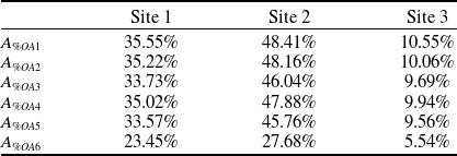
Figure 4 illustrates each site’s ROI associated with a $d = 20{\textrm{km}}$
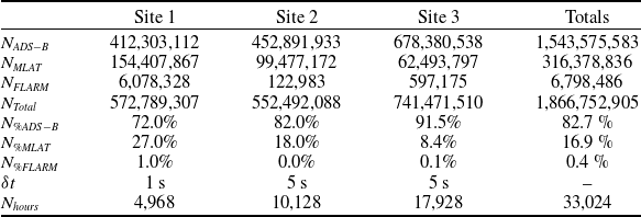
semi-length and Table 1 the relative proportion of each operating area within each ROI. Table 2 summarises the total EC reception statistics at each site.
$d = 20{\textrm{km}}$
semi-length and Table 1 the relative proportion of each operating area within each ROI. Table 2 summarises the total EC reception statistics at each site.
3.2 Aircraft types
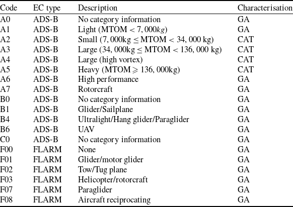
Figure 5 illustrates the number of aircraft of each category detected across all sites. Aircraft categories are defined in Table 3 along with how this study characterises them as being either GA or commercial air transport (CAT) which broadly aligns with the Type-1 and Type-2 encounters defined by UK SORA respectively.
Figure 6 illustrates the ratio of CAT aircraft to total aircraft detected across all sites, by operating area, versus height. Values significantly below 0.5 correspond to a situation where the majority of aircraft encountered are likely to be GA.
3.3 Probability of detection
Figure 7 illustrates the minimum detection height of a 1,090 MHz Mode S transponder at each site and Fig. 8 how the probability of detection for each operating area varies with height.
Percentage of each operating area present at each site

Table 1 Long description
The table presents the percentage distribution of six operating areas across three sites. It consists of seven rows and four columns, including headers. The columns are labeled Site 1, Site 2, and Site 3. The rows are labeled with operating areas A1 through A6. Notable trends include Site 2 consistently having the highest percentages across all operating areas, with values ranging from twenty-seven point sixty-eight percentage to forty-eight point forty-one percentage. Site 3 has the lowest percentages, with values ranging from five point fifty-four percentage to ten point fifty-five percentage. Site 1 has intermediate values, ranging from twenty-three point forty-five percentage to thirty-five point fifty-seven percentage. The data highlights significant variations in the distribution of operating areas across the three sites.
Summary of EC reception statistics at each site

Table 2 Long description
The table presents EC reception statistics across three sites, detailing total counts, percentages, and time intervals. It includes columns for Site 1, Site 2, Site 3, and Totals, with rows for different categories such as NADS-B, MLAT, FLARM, and Total. Each site's data is broken down into counts and percentages, along with time intervals and total hours. Notable trends include higher counts and percentages at Site 3 compared to Sites 1 and 2. The table provides a comprehensive overview of the reception statistics, highlighting variations and totals across the different sites.
Aircraft categories detected across all sites.

Figure 5 Long description
The bar graph compares the number of aircraft observed below 500 meters over built-up areas across all sites by aircraft type. The x-axis represents different aircraft categories, including A 0, A 1, A 2, A 3, A 4, A 5, A 6, A 7, B 0, B 1, B 4, B 6, C 0, F 0 0, F 0 1, F 0 2, F 0 3, F 0 7, and F 0 8. The y-axis represents the number of aircraft, ranging from 0 to 4000. The graph features two data series: General Aviation in blue and Commercial Air Traffic in red. Notable trends include high counts for A 1 and A 2 categories, with General Aviation peaking around 3300 and Commercial Air Traffic around 3600. Other categories show significantly lower counts, with some categories having no observed aircraft. The color scheme differentiates between General Aviation and Commercial Air Traffic, highlighting the distribution and frequency of aircraft types observed. All values are approximated.
Aircraft category definitions

Table 3 Long description
The table categorizes aircraft types by code, description, and characterization. It includes columns for code, EC type, description, and characterization. The codes range from A0 to F08, with descriptions such as light, small, large, heavy, rotorcraft, glider, and unmanned aerial vehicle. The characterization column specifies whether the aircraft is general aviation (GA) or commercial air transport (CAT). Notable categories include light aircraft with a maximum takeoff mass (MTOM) less than 7,000 kilograms, heavy aircraft with an MTOM of 136,000 kilograms or more, and various types of gliders and rotorcraft. The table provides a structured overview of different aircraft categories and their classifications.
Proportion of CAT aircraft detected across all sites by operating area versus height.

Figure 6 Long description
A line graph displays the proportion of commercial air transport flights within various operating areas versus height. The x-axis represents height in meters, ranging from 0 to 500 meters. The y-axis represents the proportion of flights, ranging from 0 to 1. The graph includes multiple data lines representing different operating areas: BUA, BUA - RPZ, BUA - FRZ, BUA - (RPZ+HLS500m), BUA - (FRZ+HLS500m), and BUA - (FRZ+HLS5km). Each line shows how the proportion of flights varies with height. The BUA line shows a high proportion at lower heights, peaking around 50 meters and gradually decreasing. The other lines show different patterns, with some peaking at higher heights and others showing more gradual changes. All values are approximated.
Minimum detection height at −95 dBm with a 250 W source at 1090 MHz.

Figure 7 Long description
The image contains three heat maps labeled Site 1, Site 2, and Site 3. Each heat map shows the minimum detection height at 95 dBm with a 250 W source at 1090 MHz. The heat maps use a color scale ranging from blue to red, indicating height in meters from 0 to 300. The x and y axes represent spatial dimensions, with the color intensity representing the height. Site 1 shows a central area with lower heights surrounded by higher detection heights. Site 2 has a more uniform distribution of heights with a central area of lower detection heights. Site 3 exhibits a similar pattern to Site 1 but with more pronounced variations in height detection.
Probability of ADS-B detection with height.

Figure 8 Long description
Three line graphs showing probability of detection above each operating area at three different sites. The x-axis represents height in meters ranging from 0 to 500 meters. The y-axis represents the probability of detection ranging from 0 to 1. Each graph includes multiple data lines representing different scenarios: BUA, BUA-RPZ, BUA-FRZ, BUA-(FRZ+HLS500m), BUA-(FRZ+HLS5km), and BUA-(RPZ+HLS500m). The graphs illustrate how the probability of detection increases with height for each scenario. All values are approximated.
3.4 Unmitigated MAC rate
Figure 9 illustrates the raw EC data received within each ROI. Figure 10 illustrates the unmitigated MAC rate for each operating area at each site, including an upper uncertainty bound based upon the probability of detection.
Raw data points observed below 300 m height. RPZs and 500 m HLSs shown in red.

Figure 9 Long description
The image contains three heat maps labeled Site 1, Site 2, and Site 3, each showing raw data points observed below 300 meters height. The maps use a color scale ranging from red to blue, indicating varying heights from 0 to 300 meters. Red circles mark restricted areas, and red rectangles highlight specific regions of interest. Each site displays different patterns of data distribution, with Site 1 showing a dense cluster of high-altitude data points in the upper left, Site 2 exhibiting a more dispersed pattern with several high-altitude clusters, and Site 3 featuring a central concentration of high-altitude data points. The maps provide a visual representation of the height distribution of raw data points within the specified altitude range.
Unmitigated MAC rate over different operating regions. Shaded area indicates probability of detection error.

Figure 10 Long description
The image contains three line graphs labeled Site 1, Site 2, and Site 3, each depicting the unmitigated mid-air collision rate over different operating areas. The x-axis represents height in meters, ranging from 0 to 500 meters, while the y-axis represents the collision rate. Each graph includes multiple lines representing different operating conditions, with shaded areas indicating the probability of detection error. The graphs show variations in collision rates at different heights, with notable peaks and troughs. The data suggests that collision rates vary significantly across different sites and operating conditions. All values are approximated.
4.0 DISCUSSION
The aircraft categories observed by operating area shown in Fig. 6 clearly demonstrate that outside of the RPZs the majority of aircraft encountered at low level will be GA. This observation is consistent with the nature of CAT operations, requiring that descent to lower altitudes only be conducted during a stabilised approach to a runway [33], which necessitates such operations being within an RPZ. A typical ${3^ \circ }$
CAT approach [34] will be at a height of
${3^ \circ }$
CAT approach [34] will be at a height of $5,000 \times {\textrm{tan}}$
3^
$5,000 \times {\textrm{tan}}$
3^ $ \approx 262{\textrm{ m}}$
above the threshold when entering the RPZ, which is consistent with the significant increase in non-RPZ operating areas observed around this height. It is also apparent that there is no significant difference in this result whether or not the wider ATZ is excluded which is to be expected as, away from the RPZ area, the ATZ is predominantly used by visual circuit traffic [35], which is typically at 1,000 ft AAL.
$ \approx 262{\textrm{ m}}$
above the threshold when entering the RPZ, which is consistent with the significant increase in non-RPZ operating areas observed around this height. It is also apparent that there is no significant difference in this result whether or not the wider ATZ is excluded which is to be expected as, away from the RPZ area, the ATZ is predominantly used by visual circuit traffic [35], which is typically at 1,000 ft AAL.
This result leads to the conclusion that outside of an RPZ the majority of traffic encountered by a UA at low level will be GA. Both the nature of GA operations and the lower occupancy of the aircraft themselves support the adoption of a lower TLS with regard to MAC. Specifically: a TLS of ${\lambda _{{\textrm{MAC}}}} \lt {10^{ - 7}}{\textrm{h}}{{\textrm{r}}^{ - 1}}$
as proposed by JARUS SORA [11].
${\lambda _{{\textrm{MAC}}}} \lt {10^{ - 7}}{\textrm{h}}{{\textrm{r}}^{ - 1}}$
as proposed by JARUS SORA [11].
Figures 7 and 8 illustrate that there is a significant challenge in the ability of a single ground-based EC receiver to detect aircraft at low level. The uncertainty associated with this reduced probability of detection is captured in subsequent analysis and a qualitative analysis of Fig. 7 against Fig. 9 shows that the majority of traffic flows are actually well captured. This result also demonstrates the importance of using a locally sited EC receiver when seeking to conduct quantitative airspace analysis down to low levels rather than more convenient network-based sources.
Figure 10 shows that for built-up areas without any exclusions there is a significant peak in MAC rate around 50 m, corresponding to aircraft descending on their final approach to, and/or departing from, the runway. Once the RPZs are excluded, however, these peaks significantly shifts to the right for sites 1 and 2. The difference in the height at which the peak occurs between site 1 and 2 is explained by the fact that instantaneous height above terrain (as plotted) differs from height above the threshold which should be broadly consistent between sites. Specifically, at site 1, the terrain drops away from the runway to the edge of the RPZ by approximately 100 m.
For site 3 the shift in this peak is less obvious, however, a small peak is observable within a similar height range, albeit much broader. This observation is likely explained by the fact that site 3 is located in proximity to a smaller GA airfield with lower traffic volumes and less stringent approach stabilisation criteria. This conclusion can be further evidenced by the larger difference observed between excluding only the RPZ and the entire FRZ, indicating that aircraft are operating at a lower height outside of the RPZ but still within the FRZ, likely corresponding to the crosswind and base legs of the visual traffic circuit [36]. These legs can be observed by inspection of the flight paths illustrated in Fig. 9(c).
Site 3 shows no difference in MAC rate whether or not HLS are excluded from the operating area, as Fig. 9(c) illustrates that no traffic is observed operating to these sites. Site 2 shows limited difference, again because little relevant traffic is observed.
Site 1 shows a clear distinction when HLSs are excluded, due to the presence of a relatively busy HLS in the city centre as observed in 9a. It is interesting to note, however, that even without excluding the HLS a TLS of ${\lambda _{{\textrm{MAC}}}} \lt {10^{ - 7}}{\textrm{h}}{{\textrm{r}}^{ - 1}}$
is still achieved with only an RPZ exclusion. Further, it is clear that a 500 m radius is sufficient for HLSs located within built-up areas as there is no significant difference in MAC rate between that restriction and the 5 km radius restriction.
${\lambda _{{\textrm{MAC}}}} \lt {10^{ - 7}}{\textrm{h}}{{\textrm{r}}^{ - 1}}$
is still achieved with only an RPZ exclusion. Further, it is clear that a 500 m radius is sufficient for HLSs located within built-up areas as there is no significant difference in MAC rate between that restriction and the 5 km radius restriction.
Figure 1 shows that the built-up areas associated with sites 1 and 2 are larger and more contiguous than site 3, likely making it easier for crewed aircraft pilots to recognise their boundaries and remain clear and less likely for unlicensed airfields, which are not afforded the protections of an RPZ, to be present. Additionally, the fact that the majority of sites 1 and 2 sit within controlled airspace implies a high level of EC equipage and therefore a high confidence in the MAC rate distributions presented.
In contrast, site 3 contains smaller, more disparate built-up areas; is more likely to contain unlicensed airfields; and, being uncontrolled airspace, may contain significant levels of non-EC equipped aircraft, providing less confidence in the MAC rate results presented. However, CAA data suggest that up to $78\% $
of aircraft routinely using UK airspace are EC equipped [37], therefore it is anticipated that the results presented here are representative to within an order of magnitude.
$78\% $
of aircraft routinely using UK airspace are EC equipped [37], therefore it is anticipated that the results presented here are representative to within an order of magnitude.
5.0 Conclusions
This work has presented a method for determining the likely MAC rate between UA and crewed aviation operating over built-up areas, in the context of the UK SERA, to support the quantification of AAEs in those areas. It has been shown that, outside of RPZs, the most likely encounters to occur at heights below 250 m are with GA, supporting the use of a TLS of ${\lambda _{{\textrm{MAC}}}} \lt {10^{ - 7}}{\textrm{h}}{{\textrm{r}}^{ - 1}}$
.
${\lambda _{{\textrm{MAC}}}} \lt {10^{ - 7}}{\textrm{h}}{{\textrm{r}}^{ - 1}}$
.
Further, it has been shown that within controlled airspace, outside of RPZs and 500 m away from HLSs, this TLS can be achieved with high confidence up to heights in excess of 200 m. Outside of controlled airspace, operating outside of the entire FRZ provides a similar level of confidence up to 100 m.
In reference to the definition of an AAE as an area where ‘…it can be reasonably anticipated that there will be a greatly reduced number of conventionally piloted aircraft…’ [12], and recognising the logarithmic scale of Fig. 10, it can be concluded that areas in which the TLS is achieved with a high confidence must satisfy this definition.
This study has specifically focused on the effects of RPZs and HLS due to their prevalence within the data available for analysis. Where UA operations are being considered over built up areas and in proximity to other known low-level air activities, such as defined helicopter routes [38], their effects should also be analysed.
This work has presented a worst-case scenario, assuming no additional risk mitigation being undertaken by the UA operator besides their choice of operating area. In reality any responsible UA operator should undertake additional mitigations, such as the publication of a Notice To Airmen (NOTAM) for their operation or the incorporation of EC-in to their system. Such actions will only further reduce the already acceptable MAC rate, providing a significant safety margin for UA operations.
Finally, this paper has shown how the recording of EC data within a particular ROI allows the associated airspace risks to be quantified. In order to maintain confidence in these conclusions over time, it is important that ground-based infrastructure be deployed to persistently capture all air traffic and not only those detected by a UA in flight as a part of an onboard DAA system.
Acknowledgements
The authors would like to thank Autospray Systems Ltd, British Transport Police (BTP), Network Rail (NR) and Skypointe Ltd for their contribution of EC equipment and data in support of this work. The data analysis was undertaken on Barkla, part of the High Performance Computing (HPC) facilities at the University of Liverpool, UK.


 PMSL
PMSL


 Open access