


1. Introduction
The processes of gas accretion, star formation and gas outflows are paramount in understanding how galaxies form and evolve. Accurate measurements of gas-phase chemical composition provide some of the most robust constraints on these processes (e.g. Erb et al. Reference Erb2006; Erb Reference Erb2008; Peeples & Shankar Reference Peeples and Shankar2011; Lilly et al. Reference Lilly, Carollo, Pipino, Renzini and Peng2013; Davé, Finlator, & Oppenheimer Reference Davé, Finlator and Oppenheimer2011; Davé et al. Reference Davé, Rafieferantsoa, Thompson and Hopkins2017; Sanders et al. Reference Sanders2021). Gas accretion dilutes metals in the interstellar medium (ISM), star formation produces metals through nucleosynthesis and then returns them to the ISM through supernovae and stellar winds, and outflows remove metals from galaxies. Thus, the gas-phase metallicity of a galaxy is regulated by the interplay between gas inflows, outflows, and star formation. Consequently, studies of chemical evolution serve as a powerful tool to infer the baryonic processes shaping galaxies over cosmic time.
Gas-phase oxygen abundance (referred to herein as ‘metallicity,’ expressed as $12+\log{(\mathrm{O/H})}$
) has now been measured in galaxy populations reaching
$12+\log{(\mathrm{O/H})}$
) has now been measured in galaxy populations reaching $z\gt8$
with the James Webb Space Telescope (JWST; e.g. Arellano-Córdova et al. Reference Arellano-Córdova2022; Schaerer et al. Reference Schaerer2022; Taylor, Barger, & Cowie Reference Taylor, Barger and Cowie2022; Bunker et al. Reference Bunker2023; Curti et al. Reference Curti2023; Nakajima et al. Reference Nakajima2023; Sanders et al. Reference Trump2023; Trump et al. Reference Trump2023; Sarkar et al. Reference Sarkar2025). These advancements build upon extensive earlier surveys that have mapped metallicity evolution across
$z\gt8$
with the James Webb Space Telescope (JWST; e.g. Arellano-Córdova et al. Reference Arellano-Córdova2022; Schaerer et al. Reference Schaerer2022; Taylor, Barger, & Cowie Reference Taylor, Barger and Cowie2022; Bunker et al. Reference Bunker2023; Curti et al. Reference Curti2023; Nakajima et al. Reference Nakajima2023; Sanders et al. Reference Trump2023; Trump et al. Reference Trump2023; Sarkar et al. Reference Sarkar2025). These advancements build upon extensive earlier surveys that have mapped metallicity evolution across $z \simeq 0$
–4 (e.g. Kriek et al. Reference Kriek2015; Steidel et al. Reference Steidel2014; Wisnioski et al. Reference Wisnioski2015; Stott et al. Reference Stott2016; Treu et al. Reference Treu2015; Momcheva et al. Reference Momcheva2016). These efforts have consistently found lower metallicities at higher redshifts and at lower stellar masses (e.g. Tacconi et al. Reference Tacconi2018; Sanders et al. Reference Sanders2021; Tremonti et al. Reference Tremonti2004; Cullen et al. Reference Cullen, Cirasuolo, McLure, Dunlop and Bowler2014; Curti et al. Reference Curti, Mannucci, Cresci and Maiolino2020; Troncoso et al. Reference Troncoso2014; Andrews & Martini Reference Andrews and Martini2013; Erb et al. Reference Erb2006; Maiolino et al. Reference Maiolino2008). The observed mass-metallicity relation and its evolution are primarily attributed to a mass-dependent outflow rate, and higher gas fractions at earlier cosmic epochs.
$z \simeq 0$
–4 (e.g. Kriek et al. Reference Kriek2015; Steidel et al. Reference Steidel2014; Wisnioski et al. Reference Wisnioski2015; Stott et al. Reference Stott2016; Treu et al. Reference Treu2015; Momcheva et al. Reference Momcheva2016). These efforts have consistently found lower metallicities at higher redshifts and at lower stellar masses (e.g. Tacconi et al. Reference Tacconi2018; Sanders et al. Reference Sanders2021; Tremonti et al. Reference Tremonti2004; Cullen et al. Reference Cullen, Cirasuolo, McLure, Dunlop and Bowler2014; Curti et al. Reference Curti, Mannucci, Cresci and Maiolino2020; Troncoso et al. Reference Troncoso2014; Andrews & Martini Reference Andrews and Martini2013; Erb et al. Reference Erb2006; Maiolino et al. Reference Maiolino2008). The observed mass-metallicity relation and its evolution are primarily attributed to a mass-dependent outflow rate, and higher gas fractions at earlier cosmic epochs.
The most common approach to measuring the O/H abundances relies on nebular emission lines originating in H II regions. Collisionally excited lines (CELs) from [O III] are particularly sensitive to the electron temperature ( $T_e$
). The
$T_e$
). The $T_e$
can be determined from the ratio of two CELs probing different upper energy levels (e.g. [O III]
$T_e$
can be determined from the ratio of two CELs probing different upper energy levels (e.g. [O III] ${\lambda 4363}$
/[O III]
${\lambda 4363}$
/[O III] ${\lambda 5007}$
) and used to calculate the emissivity of oxygen and other emission lines, allowing for a precise determination of O/H abundance. This technique, known as the ‘direct
${\lambda 5007}$
) and used to calculate the emissivity of oxygen and other emission lines, allowing for a precise determination of O/H abundance. This technique, known as the ‘direct $T_e$
’ method, is commonly applied to rest-frame optical observations. However, recent JWST observations of galaxies at
$T_e$
’ method, is commonly applied to rest-frame optical observations. However, recent JWST observations of galaxies at $z \gtrsim 8$
increasingly rely on rest-UV nebular emission lines (e.g. O III]
$z \gtrsim 8$
increasingly rely on rest-UV nebular emission lines (e.g. O III] $\lambda\lambda$
1661, 1666, C III]
$\lambda\lambda$
1661, 1666, C III] ${\lambda\lambda 1907, 1909}$
, C IV
${\lambda\lambda 1907, 1909}$
, C IV ${\lambda\lambda 1549, 1551}$
) to probe gas-phase properties (e.g. Curti et al. Reference Curti2025; Hayes et al. Reference Hayes2025; Hsiao et al. Reference Hsiao2025; Tang et al. Reference Méndez-Delgado2025; Arellano-Córdova et al. Reference Arellano-Córdova2026), as the optical lines are redshifted into the more observationally challenging mid-infrared, particularly observations at
${\lambda\lambda 1549, 1551}$
) to probe gas-phase properties (e.g. Curti et al. Reference Curti2025; Hayes et al. Reference Hayes2025; Hsiao et al. Reference Hsiao2025; Tang et al. Reference Méndez-Delgado2025; Arellano-Córdova et al. Reference Arellano-Córdova2026), as the optical lines are redshifted into the more observationally challenging mid-infrared, particularly observations at $z \gtrsim 10$
. Compared to the extensive optical surveys, rest-UV spectroscopic datasets at low redshift remain more limited due to atmospheric opacity below
$z \gtrsim 10$
. Compared to the extensive optical surveys, rest-UV spectroscopic datasets at low redshift remain more limited due to atmospheric opacity below $\sim3000\,\unicode{x00C5}$
and the necessary reliance on space-based facilities with limited sensitivity. Recent programmes with the Hubble Space Telescope such as the COS Legacy Archive Spectroscopic SurveY (CLASSY; Berg et al. Reference Berg2022; James et al. Reference James2022) have substantially improved the availability of high-quality UV spectra for nearby star-forming galaxies, enabling the development of UV-based nebular diagnostics and providing insights into the ionising stellar populations that shape UV line ratios. However, precise and widely calibrated
$\sim3000\,\unicode{x00C5}$
and the necessary reliance on space-based facilities with limited sensitivity. Recent programmes with the Hubble Space Telescope such as the COS Legacy Archive Spectroscopic SurveY (CLASSY; Berg et al. Reference Berg2022; James et al. Reference James2022) have substantially improved the availability of high-quality UV spectra for nearby star-forming galaxies, enabling the development of UV-based nebular diagnostics and providing insights into the ionising stellar populations that shape UV line ratios. However, precise and widely calibrated $T_e$
measurements based on UV collisionally excited lines remain comparatively scarce relative to their optical counterparts.
$T_e$
measurements based on UV collisionally excited lines remain comparatively scarce relative to their optical counterparts.
Another challenge for chemical evolution studies is that even in sensitive rest-optical spectra, two ‘direct’ methods which can be used to derive the O++/H+ nebular abundance in an H II region systematically disagree. O/H abundances from CELs using the direct- $T_e$
method are found to be systematically lower (by
$T_e$
method are found to be systematically lower (by $\sim$
0.2–0.3 dex) compared to measurements from the much fainter oxygen recombination lines (RLs). This so-called abundance discrepancy factor (ADF; e.g. Tsamis et al. Reference Tsamis, Barlow, Liu, Danziger and Storey2003; Blanc et al. Reference Blanc, Kewley, Vogt and Dopita2015; Esteban et al. Reference Esteban2009; Esteban et al. Reference Esteban2014; García-Rojas et al. Reference García-Rojas2004; García-Rojas & Esteban Reference García-Rojas and Esteban2007) is often attributed to temperature fluctuations of the gas within H II regions (Peimbert Reference Peimbert1967; García-Rojas et al. Reference García-Rojas2004). In this scenario,
$\sim$
0.2–0.3 dex) compared to measurements from the much fainter oxygen recombination lines (RLs). This so-called abundance discrepancy factor (ADF; e.g. Tsamis et al. Reference Tsamis, Barlow, Liu, Danziger and Storey2003; Blanc et al. Reference Blanc, Kewley, Vogt and Dopita2015; Esteban et al. Reference Esteban2009; Esteban et al. Reference Esteban2014; García-Rojas et al. Reference García-Rojas2004; García-Rojas & Esteban Reference García-Rojas and Esteban2007) is often attributed to temperature fluctuations of the gas within H II regions (Peimbert Reference Peimbert1967; García-Rojas et al. Reference García-Rojas2004). In this scenario, $T_e$
values measured from optical CELs are biased high resulting in the direct-
$T_e$
values measured from optical CELs are biased high resulting in the direct- $T_e$
metallicities biased low. Meanwhile, the recombination line metallicities are accurate due to their insensitivity to
$T_e$
metallicities biased low. Meanwhile, the recombination line metallicities are accurate due to their insensitivity to $T_e$
. For the UV emission lines, such as O III]
$T_e$
. For the UV emission lines, such as O III] $\lambda\lambda$
1661, 1666, this would suggest that
$\lambda\lambda$
1661, 1666, this would suggest that $T_e$
derived from rest-UV lines would be biased even higher and thus metallicities even lower compared to the optical CELs. On the other hand, another explanation of the ADF involves inclusions of high-metallicity gas (Croxall et al. Reference Croxall2013; Stasińska et al. 2007) among an ambient medium with lower metallicity, in which case the CELs are expected to be more accurate than RLs. Some studies have found good agreement between the metallicities of young stars and CEL-based nebular measurements (e.g. Bresolin et al. Reference Bresolin2016; Bresolin et al. Reference Bresolin, Kudritzki, Urbaneja, Sextl and Riess2025), suggesting that
$T_e$
derived from rest-UV lines would be biased even higher and thus metallicities even lower compared to the optical CELs. On the other hand, another explanation of the ADF involves inclusions of high-metallicity gas (Croxall et al. Reference Croxall2013; Stasińska et al. 2007) among an ambient medium with lower metallicity, in which case the CELs are expected to be more accurate than RLs. Some studies have found good agreement between the metallicities of young stars and CEL-based nebular measurements (e.g. Bresolin et al. Reference Bresolin2016; Bresolin et al. Reference Bresolin, Kudritzki, Urbaneja, Sextl and Riess2025), suggesting that $T_e$
metallicities may be more reliable. As the cause of the ADF is currently not conclusively established, empirical relationships are important to establish the relative biases between different metallicity measurement techniques, such as the joint use of UV and optical CELs.
$T_e$
metallicities may be more reliable. As the cause of the ADF is currently not conclusively established, empirical relationships are important to establish the relative biases between different metallicity measurement techniques, such as the joint use of UV and optical CELs.
Significant efforts have been made in recent years to understand the gas properties measured from UV nebular emission in the local universe (e.g. Kunth et al. Reference Kunth, Lequeux, Mas-Hesse, Terlevich, Terlevich, Franco, Terlevich and Serrano1997; Senchyna et al. Reference Senchyna2017; Senchyna et al. Reference Senchyna2020; Senchyna et al. Reference Senchyna2022; Berg et al. Reference Berg2022; Kelly et al. Reference Kelly2025). However, measuring the $T_e$
and metallicity using UV emission lines is challenging, since it requires an accurate comparison between the UV and optical fluxes (e.g. C III]
$T_e$
and metallicity using UV emission lines is challenging, since it requires an accurate comparison between the UV and optical fluxes (e.g. C III] ${\lambda\lambda 1907, 1909}$
and H I Balmer lines or using O III]
${\lambda\lambda 1907, 1909}$
and H I Balmer lines or using O III] ${\lambda 1666}$
/[O III]
${\lambda 1666}$
/[O III] ${\lambda 5007}$
to derive
${\lambda 5007}$
to derive $T_e$
.). Such comparisons often introduce systematic uncertainty from different instruments and apertures used for the UV and optical measurements (e.g. Arellano-Córdova et al. Reference Arellano-Córdova2022), in addition to highly uncertain reddening corrections. Using the CLASSY survey, Mingozzi et al. (Reference Mingozzi2022) explored the promise and limitations of combining Hubble Space Telescope (HST)/Cosmic Origins Spectrograph (COS) UV spectra and various optical spectra by matching the continuum spectra to the stellar population synthesis models. Their results suggest that the [O III]
$T_e$
.). Such comparisons often introduce systematic uncertainty from different instruments and apertures used for the UV and optical measurements (e.g. Arellano-Córdova et al. Reference Arellano-Córdova2022), in addition to highly uncertain reddening corrections. Using the CLASSY survey, Mingozzi et al. (Reference Mingozzi2022) explored the promise and limitations of combining Hubble Space Telescope (HST)/Cosmic Origins Spectrograph (COS) UV spectra and various optical spectra by matching the continuum spectra to the stellar population synthesis models. Their results suggest that the [O III] $T_e$
measured from the UV emission (via O III]
$T_e$
measured from the UV emission (via O III] $\lambda\lambda$
1661, 1666/[O III]
$\lambda\lambda$
1661, 1666/[O III] ${\lambda 5007}$
) is consistent with the optical
${\lambda 5007}$
) is consistent with the optical $T_e$
(via [O III]
$T_e$
(via [O III] ${\lambda 4363}$
/[O III]
${\lambda 4363}$
/[O III] ${\lambda 5007}$
) on average with a sample standard deviation scatter of
${\lambda 5007}$
) on average with a sample standard deviation scatter of $\sim$
1500 K (
$\sim$
1500 K ( $\sim$
10% of
$\sim$
10% of $T_e$
), in relatively good agreement, but with substantial uncertainties related to dust attenuation and other effects.
$T_e$
), in relatively good agreement, but with substantial uncertainties related to dust attenuation and other effects.
In this work, we demonstrate a novel method to achieve precise comparison between the optical and UV fluxes. A key goal is to minimise uncertainty associated with combining UV and optical features, including aperture corrections and dust attenuation. We achieve this using nebular He II emission lines, namely UV He II ${\lambda 1640}$
and optical He II
${\lambda 1640}$
and optical He II ${\lambda 4686}$
. While the ionisation source of these emission lines in H II regions is still under debate (Kehrig et al. Reference Kehrig2011; Kehrig et al. Reference Kehrig2015; Schaerer, Fragos, & Izotov Reference Schaerer, Fragos and Izotov2019; Senchyna et al. Reference Senchyna2020), the production mechanism of nebular He II emission is believed to be dominated by recombination processes (Schaerer & Vacca Reference Schaerer and Vacca1998) analogous to the H I Balmer and Paschen lines. Accordingly, the flux ratio He II
${\lambda 4686}$
. While the ionisation source of these emission lines in H II regions is still under debate (Kehrig et al. Reference Kehrig2011; Kehrig et al. Reference Kehrig2015; Schaerer, Fragos, & Izotov Reference Schaerer, Fragos and Izotov2019; Senchyna et al. Reference Senchyna2020), the production mechanism of nebular He II emission is believed to be dominated by recombination processes (Schaerer & Vacca Reference Schaerer and Vacca1998) analogous to the H I Balmer and Paschen lines. Accordingly, the flux ratio He II ${\lambda 1640}$
/He II
${\lambda 1640}$
/He II ${\lambda 4686}$ $\approx 6.99$
is expected to be nearly constant and relatively insensitive to gas density and
$\approx 6.99$
is expected to be nearly constant and relatively insensitive to gas density and $T_e$
. This provides a valuable reference to calibrate observed fluxes from different instruments at rest-frame UV and optical wavelengths. In this work, we demonstrate that this method can provide precise measurements of
$T_e$
. This provides a valuable reference to calibrate observed fluxes from different instruments at rest-frame UV and optical wavelengths. In this work, we demonstrate that this method can provide precise measurements of $T_e$
and metallicity, and examine whether gas properties measured from UV features are systematically different from equivalent optical diagnostics.
$T_e$
and metallicity, and examine whether gas properties measured from UV features are systematically different from equivalent optical diagnostics.
This paper is organised as follows. We present target galaxy selection and observations in Section 2. Section 3 describes our methodology and analysis, including flux calibration of optical and UV spectra, dust attenuation and aperture corrections, and measurements of the physical properties. We discuss the reliability of our measurements and the physical implications in Section 4. Section 5 summarises our results. Emission line analyses (including correction for dust attenuation and determination of the physical properties of the gas) are performed using Pyneb (Luridiana, Morisset, & Shaw Reference Luridiana, Morisset and Shaw2015). We adopt the collision strengths from Tayal & Zatsarinny (Reference Tayal and Zatsarinny2017) for the O++ ion and the transition probabilities for all relevant lines from Froese Fischer & Tachiev (Reference Froese Fischer and Tachiev2004) throughout this work.
Summary of target galaxy properties.

aValues for SB 2 reflect the brightest star-forming region in the central knot of the galaxy, as opposed to the (larger) entire galaxy.
bRedshifts measured from O III] $\lambda\lambda$
1661, 1666 nebular emission lines.
$\lambda\lambda$
1661, 1666 nebular emission lines.
cObtained from Senchyna et al. (Reference Senchyna2017). $M_*$
was measured from SED fitting with a typical uncertainty of 0.1 dex, and
$M_*$
was measured from SED fitting with a typical uncertainty of 0.1 dex, and $12+\log\mathrm{(O/H)}$
was measured using the optical direct
$12+\log\mathrm{(O/H)}$
was measured using the optical direct $T_e$
method.
$T_e$
method.
dObtained from Berg et al. (Reference Berg2022), where SFR was measured using Beagle SED fitting.
e $n_e$
derived from the [S II]
$n_e$
derived from the [S II] ${\lambda\lambda}$
6731/6716 flux ratio for each object.
${\lambda\lambda}$
6731/6716 flux ratio for each object.
Images of the three blue compact dwarf galaxies studied in this work. Each panel shows a SDSS u, g, r false-colour image, the HST/COS $2^{\prime\prime}5$
aperture (circles), and the Keck/ ESI 1
$2^{\prime\prime}5$
aperture (circles), and the Keck/ ESI 1 $\times$
20 slit (rectangles). The 25 COS aperture size corresponds to projected diameters of 0.23 kpc for SB 2, 0.92 kpc for SB 82, and 2.31 kpc for SB 182 (Senchyna et al. Reference Senchyna2017). Near-UV target acquisition images from COS for all three objects can be found in Reference SenchynaS17. All three objects are dwarf galaxies containing one primary H II region, from which the majority of nebular line emission is captured by both the COS and ESI apertures.
$\times$
20 slit (rectangles). The 25 COS aperture size corresponds to projected diameters of 0.23 kpc for SB 2, 0.92 kpc for SB 82, and 2.31 kpc for SB 182 (Senchyna et al. Reference Senchyna2017). Near-UV target acquisition images from COS for all three objects can be found in Reference SenchynaS17. All three objects are dwarf galaxies containing one primary H II region, from which the majority of nebular line emission is captured by both the COS and ESI apertures.

2. Sample selection and data
Here, we describe the target sample and spectroscopic data used in this work. Our sample was selected from a superset of ten metal-poor star-forming galaxies analysed in (Senchyna et al. Reference Senchyna2017, hereafter Reference SenchynaS17), which presented UV spectra of these galaxies from HST’s Cosmic Origins Spectrograph (COS) along with optical spectra from Keck’s Echelle Spectrograph and Imager (ESI; Sheinis et al. Reference Sheinis2002). These galaxies were initially selected based on the presence of prominent He II ${\lambda 4686}$
emission in their optical SDSS spectra (Shirazi & Brinchmann Reference Shirazi and Brinchmann2012). Since our objective is to characterise UV and optical nebular emisson, we restrict our analysis to the sample of galaxies exhibiting clear narrow nebular He II
${\lambda 4686}$
emission in their optical SDSS spectra (Shirazi & Brinchmann Reference Shirazi and Brinchmann2012). Since our objective is to characterise UV and optical nebular emisson, we restrict our analysis to the sample of galaxies exhibiting clear narrow nebular He II ${\lambda 1640}$
and He II
${\lambda 1640}$
and He II ${\lambda 4686}$
emission (as opposed to broad stellar wind emission) in high-resolution HST/COS and Keck/ESI spectra. The combination of optical and UV He II lines is necessary to obtain precise dust reddening and aperture corrections (see Section 3.2.2 for details).
${\lambda 4686}$
emission (as opposed to broad stellar wind emission) in high-resolution HST/COS and Keck/ESI spectra. The combination of optical and UV He II lines is necessary to obtain precise dust reddening and aperture corrections (see Section 3.2.2 for details).
The He II selection criteria result in a sample of three blue compact dwarf galaxies (BCDs) with relatively low metallicities ( $12 +$
log (O/H)
$12 +$
log (O/H) $\lt 8.1$
) and recent star formation activity. The properties of these galaxies are summarised in Table 1. Figure 1 presents optical images of the three BCDs. Below, we briefly outline the physical characteristics of each target (masses from Reference SenchynaS17):
$\lt 8.1$
) and recent star formation activity. The properties of these galaxies are summarised in Table 1. Figure 1 presents optical images of the three BCDs. Below, we briefly outline the physical characteristics of each target (masses from Reference SenchynaS17):
-
• SB 2 is a dwarf galaxy hosting multiple star-forming regions. Our analysis centres on the brightest star-forming region located in the central knot, as shown in Figure 1, which has a stellar mass of $M_* = 10^{5.1}$
M
$_{\odot}$
. This region was captured in isolation within the COS aperture (Senchyna et al. Reference Senchyna2022, hereafter Reference SenchynaS22). The values used in this work pertain exclusively to the region enclosed by the COS aperture and do not account for the contributions from neighbouring star-forming regions in the galaxy.
$M_* = 10^{5.1}$
M
$_{\odot}$
. This region was captured in isolation within the COS aperture (Senchyna et al. Reference Senchyna2022, hereafter Reference SenchynaS22). The values used in this work pertain exclusively to the region enclosed by the COS aperture and do not account for the contributions from neighbouring star-forming regions in the galaxy. -
• SB 82 is an isolated dwarf galaxy with a stellar mass of
$M_*=10^{6.4}$
M
$_{\odot}$
, also known as Mrk 193. -
• SB 182 is a dwarf galaxy with a stellar mass of
$M_* = 10^{7.3}$
M
$_{\odot}$
. Morphologically, it consists of two distinct components separated by several arcseconds. In this study, we focus on the southeast star-forming region. The angular separation between the two components is sufficient to ensure that the northwest component was not included in the spectra analysed here.


2.1. Keck/ESI
The ESI data were taken on 29 March 2016 (SB 82) and 20 January 2017 (SB 2 and SB 182). Sky conditions were clear with 0.8–1.2 arcsec seeing. The 1” slit width was used, resulting in spectralresolution $R\sim 4\,000$
(75 km s-1 FWHM) spanning 3 900–10 900 Å. To minimise aperture loss due to atmospheric dispersion, all observations were taken with a slit position near the parallactic angle (PA
$R\sim 4\,000$
(75 km s-1 FWHM) spanning 3 900–10 900 Å. To minimise aperture loss due to atmospheric dispersion, all observations were taken with a slit position near the parallactic angle (PA $=304$
for SB 2, 227 for SB 82, and 272 for SB 182). The total integration time was 2 h for SB 2 and 2.5 h for SB 82 and SB 182, split into individual exposures of 30 min each. The spectra were reduced using the ESIRedux data reduction pipeline as described in Reference SenchynaS17.
$=304$
for SB 2, 227 for SB 82, and 272 for SB 182). The total integration time was 2 h for SB 2 and 2.5 h for SB 82 and SB 182, split into individual exposures of 30 min each. The spectra were reduced using the ESIRedux data reduction pipeline as described in Reference SenchynaS17.
To improve flux calibration relative to the ESIRedux processing, we scale the continuum level of Keck/ESI spectra to match that in the fully calibrated spectra available for each target from the Sloan Digital Sky Survey (SDSS; York et al. Reference York2000). We first masked out wavelength regions around the strong emission lines, and then excluded pixels deviating more than $2\sigma$
from the running median in bins of 50 Å to mask detected spectral features. The masking of weak lines was necessary to robustly estimate the continuum due to the large number of emission lines detected (
$2\sigma$
from the running median in bins of 50 Å to mask detected spectral features. The masking of weak lines was necessary to robustly estimate the continuum due to the large number of emission lines detected ( $\gt$
100 per target) in these sensitive spectra. We then fit a univariate cubic spline to the masked spectrum to obtain a smooth model of the continuum in the ESI spectrum. We performed the same steps on the SDSS spectrum, and divide the ESI by SDSS continuum model to obtain the flux calibration scaling factor. We then scale the ESI flux and error spectra by this factor. Figure 2 shows the flux-calibrated ESI spectra of the three objects in the wavelength ranges most relevant for this work.
$\gt$
100 per target) in these sensitive spectra. We then fit a univariate cubic spline to the masked spectrum to obtain a smooth model of the continuum in the ESI spectrum. We performed the same steps on the SDSS spectrum, and divide the ESI by SDSS continuum model to obtain the flux calibration scaling factor. We then scale the ESI flux and error spectra by this factor. Figure 2 shows the flux-calibrated ESI spectra of the three objects in the wavelength ranges most relevant for this work.
Keck/ESI optical spectra of the three objects presented in this work. Prominent emission features, epecially the ones useful for this work, are labeled and marked with vertical dashed lines. All relevant features are clearly detected, including nebular He II ${\lambda 4686}$
. A broad He II component is visible in SB 82.
${\lambda 4686}$
. A broad He II component is visible in SB 82.

2.2. HST/COS
The HST/COS spectroscopic observations for the BCDs have been previously presented in Reference SenchynaS17 and Reference SenchynaS22. Here we give a brief summary. The spectra were obtained using the $2^{\prime\prime}5$
COS aperture with the G160M grating centred at 1 533 Å. For SB 2 and SB 82, the COS data were taken on 4–5 April 2020 (SB 2) and 21 November 2019 (SB 82) as part of the Cycle 26 HST-GO-15646 programme. For SB 182, the data were taken on 05 November 2015 as part of the Cycle 23 HST-GO-14168 programme. The total exposure times were 26 925.12 s for SB 2, 29 255.52 s for SB 82, and 2 624.61 s for SB 182. The spectral resolution of the COS data is
$2^{\prime\prime}5$
COS aperture with the G160M grating centred at 1 533 Å. For SB 2 and SB 82, the COS data were taken on 4–5 April 2020 (SB 2) and 21 November 2019 (SB 82) as part of the Cycle 26 HST-GO-15646 programme. For SB 182, the data were taken on 05 November 2015 as part of the Cycle 23 HST-GO-14168 programme. The total exposure times were 26 925.12 s for SB 2, 29 255.52 s for SB 82, and 2 624.61 s for SB 182. The spectral resolution of the COS data is $\sim15\,000$
. Data for all three targets were reduced using the standard Calcos pipeline,Footnote
a
with the calibration files downloaded from the Space Telescope Science Data Analysis System (STSDAS).Footnote
b
For spectral extraction, we employed the ‘TWOZONE’ algorithm. Additional details on data reduction and extraction for all three targets are provided in Reference SenchynaS17 and Reference SenchynaS22.
$\sim15\,000$
. Data for all three targets were reduced using the standard Calcos pipeline,Footnote
a
with the calibration files downloaded from the Space Telescope Science Data Analysis System (STSDAS).Footnote
b
For spectral extraction, we employed the ‘TWOZONE’ algorithm. Additional details on data reduction and extraction for all three targets are provided in Reference SenchynaS17 and Reference SenchynaS22.
3. Analysis
The objectives of this work require computing the O++ abundance from the optical [O III] ${\lambda 4959}$
/H
${\lambda 4959}$
/H $\beta$
ratio using
$\beta$
ratio using $T_e$
measured from the UV O III]
$T_e$
measured from the UV O III] ${\lambda 1666}$
/[O III]
${\lambda 1666}$
/[O III] ${\lambda 4959}$
emission line ratio, and comparing it with
${\lambda 4959}$
emission line ratio, and comparing it with $T_e$
derived from the optical [O III]
$T_e$
derived from the optical [O III] ${\lambda\lambda 4363}$
/4959 ratio. This approach requires measuring accurate line fluxes from both the UV and optical spectra. Given the different excitation energies, O III]
${\lambda\lambda 4363}$
/4959 ratio. This approach requires measuring accurate line fluxes from both the UV and optical spectra. Given the different excitation energies, O III] $\lambda\lambda$
1661,1666 is more sensitive to
$\lambda\lambda$
1661,1666 is more sensitive to $T_e$
than [O III]
$T_e$
than [O III] ${\lambda 4363}$
. Comparing these measurements can therefore provide constraints on temperature fluctuations within the ionised gas, which should cause the UV-based
${\lambda 4363}$
. Comparing these measurements can therefore provide constraints on temperature fluctuations within the ionised gas, which should cause the UV-based $T_e$
to to be biased higher than the
$T_e$
to to be biased higher than the $T_e$
derived from optical [O III]
$T_e$
derived from optical [O III] ${\lambda 4363}$
. In this section we provide a detailed description of these measurements and methodology.
${\lambda 4363}$
. In this section we provide a detailed description of these measurements and methodology.
Observed and de-reddened fluxes in units of I (H $\beta$
) = 100.
$\beta$
) = 100.

aH $\gamma$
in SB 182 is affected by a detector artifact, and was not used for optical reddening correction in this object.
$\gamma$
in SB 182 is affected by a detector artifact, and was not used for optical reddening correction in this object.
bFrom a joint fit of O III] $\lambda\lambda$
1661, 1666.
$\lambda\lambda$
1661, 1666.
cThe observed H $\beta$
fluxes before extinction correction (units:
$\beta$
fluxes before extinction correction (units: $10^{-17}\mathrm{erg\,s^{-1}cm^{-2}\unicode{x00C5}^{-1}}$
).
$10^{-17}\mathrm{erg\,s^{-1}cm^{-2}\unicode{x00C5}^{-1}}$
).
Rest-frame Keck/ESI spectra with the best-fit Gaussian profile and residual for select emission lines used in this analysis for each target. The x-axis range is 10 Å for all spectra presented in this figure and the y-axis is at a scale of $10^{-17}$
erg s-1 cm-2 Å-1. We adopt a double Gaussian profile for He II
$10^{-17}$
erg s-1 cm-2 Å-1. We adopt a double Gaussian profile for He II ${\lambda 4686}$
in SB 82, representing both the broad stellar and narrow nebular components. The broad component spans
${\lambda 4686}$
in SB 82, representing both the broad stellar and narrow nebular components. The broad component spans $\gtrsim\,100$
Å so it is not shown at the scale of this figure, but can be seen in Figure 2. All other lines are adequately fit with a single narrow component.
$\gtrsim\,100$
Å so it is not shown at the scale of this figure, but can be seen in Figure 2. All other lines are adequately fit with a single narrow component.

3.1. Emission line fluxes
3.1.1. Optical line fitting
While a large number of emission lines are detected in the Keck/ESI spectra, our analysis requires only a modest subset detected at very high signal-to-noise ratios: the H I Balmer and Paschen series, [O III] ${\lambda 4363}$
, [O III]
${\lambda 4363}$
, [O III] ${\lambda 4959}$
, He II
${\lambda 4959}$
, He II ${\lambda 4686}$
, and the density-sensitive [S II]
${\lambda 4686}$
, and the density-sensitive [S II] ${\lambda 6716}$
, 6731. We measured line fluxes by fitting Gaussian profiles superposed on a linear continuum. He II
${\lambda 6716}$
, 6731. We measured line fluxes by fitting Gaussian profiles superposed on a linear continuum. He II ${\lambda 4686}$
can have a broad component from winds of massive stars as well as a narrow nebular component, of which only the nebular component is of interest to this analysis. We thus include both a broad and narrow Gaussian component when fitting He II
${\lambda 4686}$
can have a broad component from winds of massive stars as well as a narrow nebular component, of which only the nebular component is of interest to this analysis. We thus include both a broad and narrow Gaussian component when fitting He II ${\lambda 4686}$
, but only report fluxes for the narrow nebular component. SB 2 and SB 182 display no broad component in the ESI spectra. SB 82 shows weak but detected broad He II
${\lambda 4686}$
, but only report fluxes for the narrow nebular component. SB 2 and SB 182 display no broad component in the ESI spectra. SB 82 shows weak but detected broad He II ${\lambda 4686}$
emission, with the peak flux density of the broad component
${\lambda 4686}$
emission, with the peak flux density of the broad component $\approx5\times$
smaller than the narrow peak flux density. Visual inspection of the best fits indicates that the two-Gaussian model adequately matches the observed He II
$\approx5\times$
smaller than the narrow peak flux density. Visual inspection of the best fits indicates that the two-Gaussian model adequately matches the observed He II ${\lambda 4686}$
profile in SB 82 and reliably recovers the flux of the narrow component. Table 2 gives the observed optical line fluxes relative to H
${\lambda 4686}$
profile in SB 82 and reliably recovers the flux of the narrow component. Table 2 gives the observed optical line fluxes relative to H $\beta$
, in units where I(H
$\beta$
, in units where I(H $\beta)=100$
. We show best-fit profiles to the most relevant features (namely [O III]
$\beta)=100$
. We show best-fit profiles to the most relevant features (namely [O III] ${\lambda 4363}$
, He II
${\lambda 4363}$
, He II ${\lambda 4686}$
, H
${\lambda 4686}$
, H $\beta$
, and [O III]
$\beta$
, and [O III] ${\lambda 4959}$
) in Figure 3.
${\lambda 4959}$
) in Figure 3.
We do not use the H $\alpha$
or [O III]
$\alpha$
or [O III] ${\lambda 5007}$
lines because their peaks are nonlinear or saturated in the ESI spectra. Including these lines would not significantly affect the results, as equivalent information is obtained from [O III]
${\lambda 5007}$
lines because their peaks are nonlinear or saturated in the ESI spectra. Including these lines would not significantly affect the results, as equivalent information is obtained from [O III] ${\lambda 4959}$
and numerous H I lines (most importantly H
${\lambda 4959}$
and numerous H I lines (most importantly H $\beta$
and H
$\beta$
and H $\gamma$
). We have confirmed that the optical line fluxes used in this analysis are consistent between the SDSS and ESI spectra. In this work we use the ESI data which has significantly higher signal-to-noise and spectral resolution.
$\gamma$
). We have confirmed that the optical line fluxes used in this analysis are consistent between the SDSS and ESI spectra. In this work we use the ESI data which has significantly higher signal-to-noise and spectral resolution.
3.1.2. UV line fitting
The He II ${\lambda 1640}$
, O III]
${\lambda 1640}$
, O III] ${\lambda 1661}$
, and O III]
${\lambda 1661}$
, and O III] ${\lambda 1666}$
UV emission lines were originally described in Reference SenchynaS17, based on HST/COS spectra with limited exposure times (one orbit) for all three objects. Subsequent observations with significantly longer exposure times were obtained for SB2 and SB82, reported in Reference SenchynaS22. In this work we refit the UV line fluxes using the deeper spectra from these new observations. All three lines were fit using a Gaussian profile plus a linear continuum. Milky Way interstellar absorption features were masked out where necessary. The O III]
${\lambda 1666}$
UV emission lines were originally described in Reference SenchynaS17, based on HST/COS spectra with limited exposure times (one orbit) for all three objects. Subsequent observations with significantly longer exposure times were obtained for SB2 and SB82, reported in Reference SenchynaS22. In this work we refit the UV line fluxes using the deeper spectra from these new observations. All three lines were fit using a Gaussian profile plus a linear continuum. Milky Way interstellar absorption features were masked out where necessary. The O III] ${\lambda 1666}$
and O III]
${\lambda 1666}$
and O III] ${\lambda 1661}$
lines originate from the same upper energy level, resulting in a fixed O III]
${\lambda 1661}$
lines originate from the same upper energy level, resulting in a fixed O III] ${\lambda 1666}$
/O III]
${\lambda 1666}$
/O III] ${\lambda 1661}$
flux ratio that is independent of
${\lambda 1661}$
flux ratio that is independent of $T_e$
and
$T_e$
and $n_e$
. Thus, we performed a joint fit to O III]
$n_e$
. Thus, we performed a joint fit to O III] $\lambda\lambda$
1661, 1666 with the same width and redshift for both lines, and fixing the flux ratio to the theoretically expected value of 2.49 which we calculated using Pyneb (Luridiana et al. Reference Luridiana, Morisset and Shaw2015).
$\lambda\lambda$
1661, 1666 with the same width and redshift for both lines, and fixing the flux ratio to the theoretically expected value of 2.49 which we calculated using Pyneb (Luridiana et al. Reference Luridiana, Morisset and Shaw2015).
The He II ${\lambda 1640}$
emission was fit independently from the O III]
${\lambda 1640}$
emission was fit independently from the O III] $\lambda\lambda$
1661, 1666 doublet. The redshifts measured from He II and O III] are consistent with one another for each object. While SB 82 exhibits a broad component of optical He II
$\lambda\lambda$
1661, 1666 doublet. The redshifts measured from He II and O III] are consistent with one another for each object. While SB 82 exhibits a broad component of optical He II ${\lambda 4686}$
, we do not detect significant broad He II
${\lambda 4686}$
, we do not detect significant broad He II ${\lambda 1640}$
emission. Given the flux ratio between the broad and narrow components of the optical He II
${\lambda 1640}$
emission. Given the flux ratio between the broad and narrow components of the optical He II ${\lambda 4686}$
emission, we indeed do not expect to detect the broad component in the He II
${\lambda 4686}$
emission, we indeed do not expect to detect the broad component in the He II ${\lambda 1640}$
observations (see Section 3.1.1 and Figures 2, 3). Likewise we do not detect broad He II
${\lambda 1640}$
observations (see Section 3.1.1 and Figures 2, 3). Likewise we do not detect broad He II ${\lambda 1640}$
in SB 2 and SB 182. Consequently we fit the UV He II
${\lambda 1640}$
in SB 2 and SB 182. Consequently we fit the UV He II ${\lambda 1640}$
lines with a single narrow component, which provides an adequate fit to the data. The resulting nebular emission fluxes are reported in Table 2, and lines fits are shown in Figure 4.
${\lambda 1640}$
lines with a single narrow component, which provides an adequate fit to the data. The resulting nebular emission fluxes are reported in Table 2, and lines fits are shown in Figure 4.
Binned HST/COS spectra, associated 1 $\sigma$
error spectra, best-fit Gaussian models, and residual spectra for our targets SB 2, SB 82 and SB 182. SB 2 and SB 82 have 10 orbits of COS data (Senchyna et al. Reference Senchyna2022), while SB 182 has only a single orbit (Senchyna et al. Reference Senchyna2017). Above, z is the redshift as measured from the observed UV spectra.
$\sigma$
error spectra, best-fit Gaussian models, and residual spectra for our targets SB 2, SB 82 and SB 182. SB 2 and SB 82 have 10 orbits of COS data (Senchyna et al. Reference Senchyna2022), while SB 182 has only a single orbit (Senchyna et al. Reference Senchyna2017). Above, z is the redshift as measured from the observed UV spectra. $f_{1640}$
,
$f_{1640}$
, $f_{1661}$
and
$f_{1661}$
and $f_{1666}$
are the measured flux and 1
$f_{1666}$
are the measured flux and 1 $\sigma$
uncertainty for He II
$\sigma$
uncertainty for He II ${\lambda 1640}$
, O III]
${\lambda 1640}$
, O III] ${\lambda 1661}$
and O III]
${\lambda 1661}$
and O III] ${\lambda 1666,}$
respectively. Milky Way interstellar absorption features (e.g. at rest wavelengths of approximately 1 663 Å for SB 2 and 1 642 Å for SB 82) were masked and excluded from the fitting. All emission lines used in our analysis are well-detected and unaffected by Milky Way absorption.
${\lambda 1666,}$
respectively. Milky Way interstellar absorption features (e.g. at rest wavelengths of approximately 1 663 Å for SB 2 and 1 642 Å for SB 82) were masked and excluded from the fitting. All emission lines used in our analysis are well-detected and unaffected by Milky Way absorption.

3.2. Dust and aperture corrections
Accurately measuring metallicities from UV emission lines requires reliable comparisons between the UV and optical fluxes. A key objective of this work is to evaluate the effectiveness of using He II recombination lines for dust and aperture corrections. In this section, we outline the methodology to perform these corrections.
3.2.1. Optical reddening correction
Before applying the dust and aperture corrections between the optical and UV, we first corrected the optical line flux ratios for dust attenuation. This correction was performed using the standard nebular reddening correction method based on H II Balmer and Paschen line ratios. First, multiple $E(B{-}V)$
values were calculated using the ratios of H
$E(B{-}V)$
values were calculated using the ratios of H $\gamma$
, H
$\gamma$
, H $\delta$
, and the 8 750.47, 8 862.79, 9 014.91 and 9 229.01 Å Paschen lines (P12, P11, P10, P9) relative to H
$\delta$
, and the 8 750.47, 8 862.79, 9 014.91 and 9 229.01 Å Paschen lines (P12, P11, P10, P9) relative to H $\beta$
. Our fiducial analysis assumes the Cardelli et al. (Reference Cardelli, Clayton and Mathis1989) extinction law with
$\beta$
. Our fiducial analysis assumes the Cardelli et al. (Reference Cardelli, Clayton and Mathis1989) extinction law with $R_V = 3.1$
, while alternative extinction laws and
$R_V = 3.1$
, while alternative extinction laws and $R_V$
values are discussed below in this section. Intrinsic flux ratios relative to H
$R_V$
values are discussed below in this section. Intrinsic flux ratios relative to H $\beta$
were calculated in PyNeb assuming an electron temperature
$\beta$
were calculated in PyNeb assuming an electron temperature $T_e =$
15 000 K and an electron density
$T_e =$
15 000 K and an electron density $n_e =$
175 cm-3, corresponding to typical values in our sample (Section 3.3). The final
$n_e =$
175 cm-3, corresponding to typical values in our sample (Section 3.3). The final $E(B{-}V)$
value was then calculated as the inverse-variance weighted mean of the individual
$E(B{-}V)$
value was then calculated as the inverse-variance weighted mean of the individual $E(B{-}V)$
estimates. H
$E(B{-}V)$
estimates. H $\alpha$
was not used due to saturation. The dust corrected optical fluxes normalised to I (H
$\alpha$
was not used due to saturation. The dust corrected optical fluxes normalised to I (H $\beta$
) = 100 are listed in Table 2. While we report fluxes normalised to H
$\beta$
) = 100 are listed in Table 2. While we report fluxes normalised to H $\beta$
as is standard practice, He II
$\beta$
as is standard practice, He II ${\lambda 4686}$
is the most relevant reference point for the joint analysis of optical and UV lines.
${\lambda 4686}$
is the most relevant reference point for the joint analysis of optical and UV lines.
In order to account for systematic uncertainties arising from optical dust attenuation correction, we considered several extinction laws prior to choosing the well-established Cardelli et al. (Reference Cardelli, Clayton and Mathis1989) curve for our analysis. Additionally, we use a range of H-Balmer and Paschen lines for the correction, which cover the spectral range of $\sim$
4 100–9 200 Å. The relative reddening correction between [O III]
$\sim$
4 100–9 200 Å. The relative reddening correction between [O III] ${\lambda 4959}$
and [O III]
${\lambda 4959}$
and [O III] ${\lambda 4363}$
, which both fall well within the range covered by the hydrogen lines, should not be sensitive to the choice of reddening curve. We tested three curves (Cardelli et al. Reference Cardelli, Clayton and Mathis1989; Calzetti et al. Reference Calzetti2000; Gordon et al. Reference Gordon, Clayton, Misselt, Landolt and Wolff2003) with varying
${\lambda 4363}$
, which both fall well within the range covered by the hydrogen lines, should not be sensitive to the choice of reddening curve. We tested three curves (Cardelli et al. Reference Cardelli, Clayton and Mathis1989; Calzetti et al. Reference Calzetti2000; Gordon et al. Reference Gordon, Clayton, Misselt, Landolt and Wolff2003) with varying $R_v = 3.1$
–
$R_v = 3.1$
– $4.1$
. The change in the [O III]
$4.1$
. The change in the [O III] ${\lambda 4363}$
/[O III]
${\lambda 4363}$
/[O III] ${\lambda 4959}$
ratio is within 0.7% of our fiducial choice.
${\lambda 4959}$
ratio is within 0.7% of our fiducial choice.
3.2.2. UV reddening and aperture correction
Dust attenuation laws exhibit significant variation in the ultraviolet (e.g. Cardelli et al. Reference Cardelli, Clayton and Mathis1989; Calzetti et al. Reference Calzetti2000; Gordon et al. Reference Gordon, Clayton, Misselt, Landolt and Wolff2003), introducing substantial systematic uncertainties in UV-to-optical line ratios (e.g. O III] ${\lambda 1666}$
/[O III]
${\lambda 1666}$
/[O III] ${\lambda 4959}$
). Furthermore, differences in the acquisition apertures and point-spread functions between the Keck/ESI and HST/COS spectra complicate direct comparisons. By leveraging the UV He II
${\lambda 4959}$
). Furthermore, differences in the acquisition apertures and point-spread functions between the Keck/ESI and HST/COS spectra complicate direct comparisons. By leveraging the UV He II ${\lambda 1640}$
and optical He II
${\lambda 1640}$
and optical He II ${\lambda 4686}$
recombination lines, both issues are simultaneously addressed.
${\lambda 4686}$
recombination lines, both issues are simultaneously addressed.
The intrinsic flux ratio He II ${\lambda 1640}$
/He II
${\lambda 1640}$
/He II ${\lambda 4686}$ $= 6.99$
(He II
$= 6.99$
(He II ${\lambda 4686}$
/He II
${\lambda 4686}$
/He II ${\lambda 1640}$ $= 0.143$
) at
$= 0.143$
) at $T_e = 15\,000$
K and
$T_e = 15\,000$
K and $n_e = 175$
cm−
3, and is relatively insensitive to variations in
$n_e = 175$
cm−
3, and is relatively insensitive to variations in $T_e$
and
$T_e$
and $n_e$
over the range of temperatures we investigate, making this ratio a reliable tool for correcting dust reddening between UV and optical nebular lines. This approach is similar to the use of H i line ratios in correcting optical attenuation. (We note that while the He II
$n_e$
over the range of temperatures we investigate, making this ratio a reliable tool for correcting dust reddening between UV and optical nebular lines. This approach is similar to the use of H i line ratios in correcting optical attenuation. (We note that while the He II ${\lambda 4686}$
/He II
${\lambda 4686}$
/He II ${\lambda 1640}$
ratio is relatively stable, it is more affected by
${\lambda 1640}$
ratio is relatively stable, it is more affected by $T_e$
than H I. We address this concern later in this section.) After the optical lines have been corrected for dust reddening (as described in Section 3.2.1), the reddening-corrected and aperture-matched He II
$T_e$
than H I. We address this concern later in this section.) After the optical lines have been corrected for dust reddening (as described in Section 3.2.1), the reddening-corrected and aperture-matched He II ${\lambda 1640}$
flux can be determined by comparing the observed He II
${\lambda 1640}$
flux can be determined by comparing the observed He II ${\lambda 4686}$
/He II
${\lambda 4686}$
/He II ${\lambda 1640}$
flux ratio to its intrinsic value. The correction factor
${\lambda 1640}$
flux ratio to its intrinsic value. The correction factor $f_{c}$
can be expressed as
$f_{c}$
can be expressed as
 \begin{equation} {f_c} = \left({\mathrm{\frac{He\,{II}\,4686_{\,corr\,}}{He\,{II}\,1640_{\,unc}}}}\right)_\mathrm{obs} \times\, \left({\mathrm{\frac{ He\,{II}\,1640}{He\,{II}\,4686}}}\right)_\mathrm{int},\end{equation}
where He II ${{\lambda 4686}}_\mathrm{corr}$
is the dust-corrected He II
${{\lambda 4686}}_\mathrm{corr}$
is the dust-corrected He II ${\lambda 4686}$
flux, He II
${\lambda 4686}$
flux, He II ${\lambda 1640}$ $_\mathrm{unc}$
is the uncorrected observed He II
$_\mathrm{unc}$
is the uncorrected observed He II ${\lambda 1640}$
flux, and (He II
${\lambda 1640}$
flux, and (He II ${\lambda 1640}$
/He II
${\lambda 1640}$
/He II ${\lambda 4686}$
)
${\lambda 4686}$
) $_\mathrm{int}$
is the intrinsic flux ratio between the two lines.
$_\mathrm{int}$
is the intrinsic flux ratio between the two lines.
Measured $T_e$
,
$T_e$
, $T_0$
, and
$T_0$
, and $t^2$
values for SB 82, SB 182, and SB 2. We note that variances
$t^2$
values for SB 82, SB 182, and SB 2. We note that variances $t^2 \lt 0$
are formally unphysical.
$t^2 \lt 0$
are formally unphysical.

Once this correction factor is determined, it can be applied to the O III] ${\lambda 1666}$
and O III]
${\lambda 1666}$
and O III] ${\lambda 1661}$
lines. Since the O III]
${\lambda 1661}$
lines. Since the O III] ${\lambda 1666}$
, O III]
${\lambda 1666}$
, O III] ${\lambda 1661}$
doublet and He II
${\lambda 1661}$
doublet and He II ${\lambda 1640}$
are relatively close in wavelength, the variation in the correction factor between these lines is minimal. For the Cardelli et al. (Reference Cardelli, Clayton and Mathis1989) extinction curve with
${\lambda 1640}$
are relatively close in wavelength, the variation in the correction factor between these lines is minimal. For the Cardelli et al. (Reference Cardelli, Clayton and Mathis1989) extinction curve with $R_V = 3.1$
and
$R_V = 3.1$
and $E(B{-}V) = 0.167$
(the maximum
$E(B{-}V) = 0.167$
(the maximum $E(B{-}V)$
value among the three objects), the correction factor changes by only 0.5% between O III]
$E(B{-}V)$
value among the three objects), the correction factor changes by only 0.5% between O III] ${\lambda 1666}$
and He II
${\lambda 1666}$
and He II ${\lambda 1640}$
. For the Calzetti et al. (Reference Calzetti2000) curve with
${\lambda 1640}$
. For the Calzetti et al. (Reference Calzetti2000) curve with $R_V = 3.1$
, the difference in correction factor is only 1% and for the Gordon et al. (Reference Gordon, Clayton, Misselt, Landolt and Wolff2003) curve with
$R_V = 3.1$
, the difference in correction factor is only 1% and for the Gordon et al. (Reference Gordon, Clayton, Misselt, Landolt and Wolff2003) curve with $R_V = 3.41$
(2.74), the difference is only 0.2% (0.15%). This difference is well within the uncertainties of our analysis, regardless of the chosen attenuation curve. Thus, we apply the He II-based correction factor to the UV O III]
$R_V = 3.41$
(2.74), the difference is only 0.2% (0.15%). This difference is well within the uncertainties of our analysis, regardless of the chosen attenuation curve. Thus, we apply the He II-based correction factor to the UV O III] $\lambda\lambda$
1661, 1666 emission lines via
$\lambda\lambda$
1661, 1666 emission lines via
 \begin{equation} {F_{\lambda i\,(corr)} = {F_{\lambda i\,{\rm (unc)}}}\, \times\,} {f_c},\end{equation}
where ${F}_{\lambda i\,{\rm (corr)}}$
and
${F}_{\lambda i\,{\rm (corr)}}$
and $\mathrm{F}_{\lambda i\,{\rm (unc)}}$
are then the corrected and uncorrected fluxes for transition i, respectively. The corrected UV line fluxes are reported in units of I(H
$\mathrm{F}_{\lambda i\,{\rm (unc)}}$
are then the corrected and uncorrected fluxes for transition i, respectively. The corrected UV line fluxes are reported in units of I(H $\beta$
) = 100 in Table 2.
$\beta$
) = 100 in Table 2.
While the intrinsic He II ${\lambda 4686}$
/He II
${\lambda 4686}$
/He II ${\lambda 1640}$
flux ratio is relatively stable, it does exhibit a slight dependence on
${\lambda 1640}$
flux ratio is relatively stable, it does exhibit a slight dependence on $T_e$
, which could introduce systematic biases into our analysis. The relationship between
$T_e$
, which could introduce systematic biases into our analysis. The relationship between $T_e$
in different ionic gas regions, including between He
$T_e$
in different ionic gas regions, including between He $^+$
and O++ zones, remains an active topic of investigation (e.g. Esteban et al. Reference Esteban2014; Kreckel et al. Reference Kreckel2022; Rickards Vaught et al. Reference Rickards Vaught2024). Furthermore, nebular zones with different degrees of ionisation may be correlated with different levels of temperature fluctuations (Méndez-Delgado et al. Reference Méndez-Delgado2022). To account for this, we incorporate a systematic uncertainty of
$^+$
and O++ zones, remains an active topic of investigation (e.g. Esteban et al. Reference Esteban2014; Kreckel et al. Reference Kreckel2022; Rickards Vaught et al. Reference Rickards Vaught2024). Furthermore, nebular zones with different degrees of ionisation may be correlated with different levels of temperature fluctuations (Méndez-Delgado et al. Reference Méndez-Delgado2022). To account for this, we incorporate a systematic uncertainty of $\pm$
4 000 K in the He II
$\pm$
4 000 K in the He II $T_e$
when deriving the correction factor. This choice is motivated by the typical
$T_e$
when deriving the correction factor. This choice is motivated by the typical $T_e$
differences observed between low-ionisation (e.g. [O II]) and high-ionisation (e.g. [O III]) zones in low-metallicity, high-ionisation H II regions (e.g. Rickards Vaught et al. Reference Rickards Vaught2024). This uncertainty is added in quadrature to the UV emission line flux measurement uncertainties. The weight that this uncertainty carries in our final results varies by object. Error on the quantification of temperature fluctuations in our final results (see Section 4.1: Temperature Fluctuations) for SB 2 and SB 182 is not substantially affected by the uncertainty introduced by the intrinsic He II
$T_e$
differences observed between low-ionisation (e.g. [O II]) and high-ionisation (e.g. [O III]) zones in low-metallicity, high-ionisation H II regions (e.g. Rickards Vaught et al. Reference Rickards Vaught2024). This uncertainty is added in quadrature to the UV emission line flux measurement uncertainties. The weight that this uncertainty carries in our final results varies by object. Error on the quantification of temperature fluctuations in our final results (see Section 4.1: Temperature Fluctuations) for SB 2 and SB 182 is not substantially affected by the uncertainty introduced by the intrinsic He II ${\lambda 4686}$
/He II
${\lambda 4686}$
/He II ${\lambda 1640}$
ratio because uncertainty from flux measurements dominates. However, for SB 82, the error introduced by the temperature dependence of the correction factor is co-dominant with the UV flux error (i.e. signal-to-noise) and accounts for approximately 30% of the
${\lambda 1640}$
ratio because uncertainty from flux measurements dominates. However, for SB 82, the error introduced by the temperature dependence of the correction factor is co-dominant with the UV flux error (i.e. signal-to-noise) and accounts for approximately 30% of the $t^2$
error budget.
$t^2$
error budget.
Our measurements of $T_{e\,1666}$
versus
$T_{e\,1666}$
versus $T_{e\,4363}$
for the objects in our sample, along with measurements from Mingozzi et al. (Reference Mingozzi2022) which used a different methodology. Two galaxies in our sample (SB 2 and SB 182) have
$T_{e\,4363}$
for the objects in our sample, along with measurements from Mingozzi et al. (Reference Mingozzi2022) which used a different methodology. Two galaxies in our sample (SB 2 and SB 182) have $T_{e\,1666}+\lt+T_{e\,4363}$
, whereas temperature fluctuations predict the opposite result. Our sample displays a tight distribution with standard deviation scatter of 515 K (
$T_{e\,1666}+\lt+T_{e\,4363}$
, whereas temperature fluctuations predict the opposite result. Our sample displays a tight distribution with standard deviation scatter of 515 K ( $4.2\%$
mean absolute percent offset), while the Mingozzi et al. (Reference Mingozzi2022) sample has a larger scatter of 1557 K (
$4.2\%$
mean absolute percent offset), while the Mingozzi et al. (Reference Mingozzi2022) sample has a larger scatter of 1557 K ( $9.2\%$
mean absolute percent offset). The improved precision demonstrates success in reducing the uncertainties associated with UV attenuation corrections using our He II method (see Section 3.2.2).
$9.2\%$
mean absolute percent offset). The improved precision demonstrates success in reducing the uncertainties associated with UV attenuation corrections using our He II method (see Section 3.2.2).

3.3. Measurement of O++ electron temperature
To measure the O++ abundance, the electron temperature ( $T_e$
) of the ionised gas must first be determined in order to calculate the emissivity of the [O III] emission lines. The
$T_e$
) of the ionised gas must first be determined in order to calculate the emissivity of the [O III] emission lines. The $T_e$
can be derived from the ratio of collisionally excited lines originating from different upper energy levels (e.g. Osterbrock & Ferland Reference Osterbrock and Ferland2006). In this work we obtain two measurements of
$T_e$
can be derived from the ratio of collisionally excited lines originating from different upper energy levels (e.g. Osterbrock & Ferland Reference Osterbrock and Ferland2006). In this work we obtain two measurements of $T_e$
for each object using the dust-corrected flux ratios [O III]
$T_e$
for each object using the dust-corrected flux ratios [O III] ${\lambda\lambda 4363}$
/4959 and O III]
${\lambda\lambda 4363}$
/4959 and O III] ${\lambda 1666}$
/[O III]
${\lambda 1666}$
/[O III] ${\lambda 4959}$
, hereafter referred to as
${\lambda 4959}$
, hereafter referred to as $T_{e\,4363}$
and
$T_{e\,4363}$
and $T_{e\,1666}$
, respectively. The
$T_{e\,1666}$
, respectively. The $^{1}D_2 \rightarrow ^{3}P_1$
energy level transition produces the [O III]
$^{1}D_2 \rightarrow ^{3}P_1$
energy level transition produces the [O III] ${\lambda 4959}$
emission line,
${\lambda 4959}$
emission line, $^{1}S_0 \rightarrow ^{1}D_2$
produces [O III]
$^{1}S_0 \rightarrow ^{1}D_2$
produces [O III] ${\lambda 4363}$
, and
${\lambda 4363}$
, and $^{5}S_2^o \rightarrow ^{1}D_2$
produces O III]
$^{5}S_2^o \rightarrow ^{1}D_2$
produces O III] ${\lambda 1666}$
. Each transition samples a different upper energy level for the O++ ion, which consequently sample different collisional energies and are therefore sensitive to the electron temperature of the gas.
${\lambda 1666}$
. Each transition samples a different upper energy level for the O++ ion, which consequently sample different collisional energies and are therefore sensitive to the electron temperature of the gas.
The $T_e$
calculations were performed in Pyneb. While this requires an input of the electron density (
$T_e$
calculations were performed in Pyneb. While this requires an input of the electron density ( $n_e$
), both the optical and UV [O III] emission lines essentially have no dependence on
$n_e$
), both the optical and UV [O III] emission lines essentially have no dependence on $n_e$
across the typical range found in H II regions, since their critical densities for collisional de-excitation are
$n_e$
across the typical range found in H II regions, since their critical densities for collisional de-excitation are $\gg+1000\,\mathrm{cm}^{-3}$
. For this work we adopt
$\gg+1000\,\mathrm{cm}^{-3}$
. For this work we adopt $n_e$
values derived from the [S II]
$n_e$
values derived from the [S II] ${\lambda\lambda}$
6731/6716 line ratio, which yields
${\lambda\lambda}$
6731/6716 line ratio, which yields $n_e$
= 158, 189, 184 cm-3 for SB 2, SB 82, and SB 182, respectively (Table 1).
$n_e$
= 158, 189, 184 cm-3 for SB 2, SB 82, and SB 182, respectively (Table 1).
We consider the possibility that the choice of atomic data may influence the measurements of $T_e$
. This can in turn affect determinations of
$T_e$
. This can in turn affect determinations of $t^2$
and
$t^2$
and $T_0$
(see Section 4.1), as well as abundances measured using the
$T_0$
(see Section 4.1), as well as abundances measured using the $T_e$
method. As such, measurements for
$T_e$
method. As such, measurements for $T_e$
and the
$T_e$
and the $t^2$
analysis presented in this work were run using three different collisional strength data sets for O++ (Aggarwal & Keenan Reference Aggarwal and Keenan1999; Tayal & Zatsarinny Reference Tayal and Zatsarinny2017; Mao, Badnell, & Del Zanna Reference Mao, Badnell and Del Zanna2021). We note that Mao et al. (Reference Mao, Badnell and Del Zanna2021) produced higher values for individual
$t^2$
analysis presented in this work were run using three different collisional strength data sets for O++ (Aggarwal & Keenan Reference Aggarwal and Keenan1999; Tayal & Zatsarinny Reference Tayal and Zatsarinny2017; Mao, Badnell, & Del Zanna Reference Mao, Badnell and Del Zanna2021). We note that Mao et al. (Reference Mao, Badnell and Del Zanna2021) produced higher values for individual $T_{e\,4363}$
and
$T_{e\,4363}$
and $T_{e\,1666}$
measurements, but remain consistent within the uncertainties of the results obtained when adopting other collisional datasets. Additionally, the difference between the two quantities was the same as those from other data sets, and as such, values for
$T_{e\,1666}$
measurements, but remain consistent within the uncertainties of the results obtained when adopting other collisional datasets. Additionally, the difference between the two quantities was the same as those from other data sets, and as such, values for $t^2$
were not affected by the high individual temperature measurements. We conclude that the choice of atomic data does not significantly affect
$t^2$
were not affected by the high individual temperature measurements. We conclude that the choice of atomic data does not significantly affect $t^2$
results and adopt Tayal & Zatsarinny (Reference Tayal and Zatsarinny2017) collisional strengths throughout this analysis.
$t^2$
results and adopt Tayal & Zatsarinny (Reference Tayal and Zatsarinny2017) collisional strengths throughout this analysis.
The derived $T_{e\,4363}$
and
$T_{e\,4363}$
and $T_{e\,1666}$
are reported in Table 3. Figure 5 compares their relation with similar measurements by (Mingozzi et al. Reference Mingozzi2022, hereafter Reference MingozziM22), who found rough agreement between the two values. Our results produce a similar distribution along the 1:1 line. Although our sample contains only three galaxies, our measurements have smaller scatter about the 1:1 line compared to Reference MingozziM22. Our
$T_{e\,1666}$
are reported in Table 3. Figure 5 compares their relation with similar measurements by (Mingozzi et al. Reference Mingozzi2022, hereafter Reference MingozziM22), who found rough agreement between the two values. Our results produce a similar distribution along the 1:1 line. Although our sample contains only three galaxies, our measurements have smaller scatter about the 1:1 line compared to Reference MingozziM22. Our $T_e$
measurements have a standard deviation scatter of 515 K and a mean absolute percent offset of 4.2%, while the points from Reference MingozziM22 have a standard deviation scatter of 1 557 K and a 9.2% mean absolute percent offset. While this smaller scatter may arise in part from the small-sample statistics, or the narrower dynamic range of our sample properties, at face value it suggests that using He II emission lines for reddening and aperture corrections between the UV and optical provides more precise results.
$T_e$
measurements have a standard deviation scatter of 515 K and a mean absolute percent offset of 4.2%, while the points from Reference MingozziM22 have a standard deviation scatter of 1 557 K and a 9.2% mean absolute percent offset. While this smaller scatter may arise in part from the small-sample statistics, or the narrower dynamic range of our sample properties, at face value it suggests that using He II emission lines for reddening and aperture corrections between the UV and optical provides more precise results.
Ion abundances 12+log(O++/H+) measured from [O III] ${\lambda 4959}$
/H
${\lambda 4959}$
/H $\beta$
using different
$\beta$
using different $T_e$
values. In the absence of temperature fluctuations, we would expect
$T_e$
values. In the absence of temperature fluctuations, we would expect $T_{e\,4363}$
=
$T_{e\,4363}$
= $T_{e\,1666}$
=
$T_{e\,1666}$
= $T_0$
, with the results reflecting the true abundance for the region. Temperature fluctuations result in the abundance being higher for the
$T_0$
, with the results reflecting the true abundance for the region. Temperature fluctuations result in the abundance being higher for the $T_0$
case. Results where the
$T_0$
case. Results where the $T_0$
abundance is lower are formally unphysical (corresponding to a negative variance in temperature).
$T_0$
abundance is lower are formally unphysical (corresponding to a negative variance in temperature).

Emissivity coefficients $A_i$
,
$A_i$
, $B_i$
, and
$B_i$
, and $C_i$
for each transition.
$C_i$
for each transition.

Notes: Coefficients were found assuming $n_e = 177 \,\mathrm{cm^{-3}}$
(average electron density of the three objects used in this work; see Section 3.3). We note that the
$n_e = 177 \,\mathrm{cm^{-3}}$
(average electron density of the three objects used in this work; see Section 3.3). We note that the $C_i$
obtained are listed here but are not used directly in analysis, as the
$C_i$
obtained are listed here but are not used directly in analysis, as the $C_i$
values for each transition cancel with one another in the final relationship as expressed in Equations (4) and (6).
$C_i$
values for each transition cancel with one another in the final relationship as expressed in Equations (4) and (6).
3.4. Ionic oxygen abundance
Using the $T_e$
values calculated above and reported in Table 3, we can derive the O++/H+ abundance for each object by comparing the flux of [O III] and H I lines (namely [O III]
$T_e$
values calculated above and reported in Table 3, we can derive the O++/H+ abundance for each object by comparing the flux of [O III] and H I lines (namely [O III] ${\lambda 4959}$
/H
${\lambda 4959}$
/H $\beta$
which gives the most precise result). In this work, we provide three sets of oxygen abundances in the form of
$\beta$
which gives the most precise result). In this work, we provide three sets of oxygen abundances in the form of $12 + log({{\rm O}^{++}}/{{\rm H}^{+}}$
). The ‘UV abundance’ is derived using the dust-corrected [O III]
$12 + log({{\rm O}^{++}}/{{\rm H}^{+}}$
). The ‘UV abundance’ is derived using the dust-corrected [O III] ${\lambda 4959}$
/H
${\lambda 4959}$
/H $\beta$
ratio with
$\beta$
ratio with $T_{e\,1666}$
. The optical abundance is from the [O III]
$T_{e\,1666}$
. The optical abundance is from the [O III] ${\lambda 4959}$
/H
${\lambda 4959}$
/H $\beta$
ratio using
$\beta$
ratio using $T_{e\,4363}$
, equivalent to the classical direct-
$T_{e\,4363}$
, equivalent to the classical direct- $T_e$
method performed with optical spectra. For our sample, the optical and UV metallicities agree with each other to within 0.1 dex. This is a direct result of a nearly 1-to-1 ratio in the
$T_e$
method performed with optical spectra. For our sample, the optical and UV metallicities agree with each other to within 0.1 dex. This is a direct result of a nearly 1-to-1 ratio in the $T_{e, 1666}$
vs.
$T_{e, 1666}$
vs. $T_{e, 4363}$
relation (Figure 5). We additionally report third set of 12 + log(O++/H+) values considering the effect of temperature fluctuations (see Section 4.1 for details). The results of all three methods are provided in Table 4.
$T_{e, 4363}$
relation (Figure 5). We additionally report third set of 12 + log(O++/H+) values considering the effect of temperature fluctuations (see Section 4.1 for details). The results of all three methods are provided in Table 4.
4. Discussion
4.1. Temperature fluctuations
Since the UV O III] $\lambda\lambda$
1661, 1666 and the optical [O III]
$\lambda\lambda$
1661, 1666 and the optical [O III] ${\lambda 4959}$
and 4363 lines have different sensitivity to
${\lambda 4959}$
and 4363 lines have different sensitivity to $T_e$
, the discrepancy between the measured
$T_e$
, the discrepancy between the measured $T_e$
in these lines can in principle be used to determine the temperature fluctuations.
$T_e$
in these lines can in principle be used to determine the temperature fluctuations.
We follow the formalism of Peimbert (Reference Peimbert1967) to derive the strength of temperature fluctuations. In this framework, the temperature structure of a gaseous nebula can be characterised by two parameters: the average temperature $T_0$
and the dimensionless root mean square temperature fluctuation t2
, where
$T_0$
and the dimensionless root mean square temperature fluctuation t2
, where $t^2$
is then the temperature variance (Peimbert & Peimbert Reference Peimbert and Peimbert2013):
$t^2$
is then the temperature variance (Peimbert & Peimbert Reference Peimbert and Peimbert2013):
 \begin{align} & {T_0(\mathrm{O^{++}}) = \frac{\int_{}^{} T_e n_e n(\mathrm{O^{++}})dV} {\int_{}^{} n_e n(\mathrm{O^{++}})dV}, } \end{align}
 \begin{align} & {t^2(\mathrm{O^{++}}) = \frac{\int_{}^{} (T_e - T_0(\mathrm{O^{++}}))^2 n_e n(\mathrm{O^{++}})dV} {T_0(\mathrm{O^{++}})^2 \int_{}^{} n_e n(\mathrm{O^{++}})dV}. }\end{align}
For a single ion (in this case O++), the $T_0$
and
$T_0$
and $t^2$
can be derived from two independent measurements of
$t^2$
can be derived from two independent measurements of $T_e$
. Essentially, transitions from higher energy levels (e.g. O III]
$T_e$
. Essentially, transitions from higher energy levels (e.g. O III] ${\lambda 1666}$
compared to [O III]
${\lambda 1666}$
compared to [O III] ${\lambda 4363}$
) are biased toward higher temperatures, resulting in higher
${\lambda 4363}$
) are biased toward higher temperatures, resulting in higher $T_e$
derived using the standard approach (i.e.
$T_e$
derived using the standard approach (i.e. $T_{e\,1666}$ $\gt$
$\gt$ $T_{e\,4363}$
when
$T_{e\,4363}$
when $t^2 \gt 0$
). This difference in derived
$t^2 \gt 0$
). This difference in derived $T_e$
increases with
$T_e$
increases with $t^2$
. Assuming that the level of temperature fluctuations is relatively small compared to the average temperature
$t^2$
. Assuming that the level of temperature fluctuations is relatively small compared to the average temperature $T_0$
(i.e.
$T_0$
(i.e. $t^2 \ll 1$
), the measured electron temperatures can be Taylor expanded around the
$t^2 \ll 1$
), the measured electron temperatures can be Taylor expanded around the $T_0$
, and the relationship between
$T_0$
, and the relationship between $t^2$
,
$t^2$
, $T_0$
and
$T_0$
and $T_e$
can be expressed as
$T_e$
can be expressed as
 \begin{equation} T_{e,(\lambda1/\lambda2)} = T_0\left[1 + T_0 \left(\frac{\frac{\varepsilon^{''}_{\lambda1}(T_0)}{\varepsilon_{\lambda1}(T_0)}-\frac{\varepsilon^{''}_{\lambda2}(T_0)}{\varepsilon_{\lambda2}(T_0)}} {\frac{\varepsilon^{'}_{\lambda1}(T_0)}{\varepsilon_{\lambda1}(T_0)}-\frac{\varepsilon^{'}_{\lambda2}(T_0)}{\varepsilon_{\lambda2}(T_0)}}\right) {\frac{t^2}{2}}\right]\end{equation}
as derived by Peimbert & Peimbert (Reference Peimbert and Peimbert2013). Here $T_{e, (\lambda1\,/\,\lambda2)}$
represents the electron temperature measured from the flux ratio of two emission lines,
$T_{e, (\lambda1\,/\,\lambda2)}$
represents the electron temperature measured from the flux ratio of two emission lines, $\lambda1$
and
$\lambda1$
and $\lambda2$
. The quantity
$\lambda2$
. The quantity $\varepsilon_{\lambda 1} (T_0)$
is the emissivity of
$\varepsilon_{\lambda 1} (T_0)$
is the emissivity of $\lambda 1$
at temperature
$\lambda 1$
at temperature $T_0$
.
$T_0$
. $\varepsilon^{'}_i$
and
$\varepsilon^{'}_i$
and $\varepsilon^{''}_i$
represent the first and second derivatives of
$\varepsilon^{''}_i$
represent the first and second derivatives of $\varepsilon$
as a function of
$\varepsilon$
as a function of $T_e$
.
$T_e$
.
For collisionally excited lines, the emissivity as a function of $T_e$
can be approximated as
$T_e$
can be approximated as
 \begin{equation} \,\,\varepsilon_{\lambda}(T_e) = C_{\lambda} T_e^{-A_\lambda} \mathrm{exp}({-}B_\lambda/T_e)\,,\end{equation}
where $A_{\lambda}$
,
$A_{\lambda}$
, $B_{\lambda}$
and
$B_{\lambda}$
and $C_{\lambda}$
are coefficients for the emission line represented by
$C_{\lambda}$
are coefficients for the emission line represented by $\lambda$
(Osterbrock & Ferland Reference Osterbrock and Ferland2006). We find the coefficients for each line of interest by fitting Equation (5) to the emissivity curve derived from PyNeb within the range
$\lambda$
(Osterbrock & Ferland Reference Osterbrock and Ferland2006). We find the coefficients for each line of interest by fitting Equation (5) to the emissivity curve derived from PyNeb within the range $T_e = 5\,000$
–
$T_e = 5\,000$
– $20\,000$
K with
$20\,000$
K with $n_e = 177$
cm-3 (i.e. the average
$n_e = 177$
cm-3 (i.e. the average $n_e$
found in Section 3.3). The value of
$n_e$
found in Section 3.3). The value of $n_e$
has negligible effect given the high critical densities of the relevant lines. For the O++ lines of interest in this work, we find that
$n_e$
has negligible effect given the high critical densities of the relevant lines. For the O++ lines of interest in this work, we find that $A_\lambda = 0.4$
provides an adequate approximation and adopt this as a fixed parameter. The assumed
$A_\lambda = 0.4$
provides an adequate approximation and adopt this as a fixed parameter. The assumed $A_\lambda$
and best-fit
$A_\lambda$
and best-fit $B_\lambda$
and
$B_\lambda$
and $C_\lambda$
are listed in Table 5. The fitted functions reproduce the emissivities from PyNeb within 2%.
$C_\lambda$
are listed in Table 5. The fitted functions reproduce the emissivities from PyNeb within 2%.
With the coefficients in Table 5, we apply Equations (4) and (5) with the measured values of $T_{e\,1666}$
and
$T_{e\,1666}$
and $T_{e\,4363}$
from our targets. The dimensionless variance
$T_{e\,4363}$
from our targets. The dimensionless variance $t^2$
is directly proportional to the discrepancy between these two temperatures, and can be expressed as
$t^2$
is directly proportional to the discrepancy between these two temperatures, and can be expressed as
 \begin{equation} \,\,t^2\,(T_{e\,4363},T_{e\,1666})\, = \frac{2}{B_{4363}-B_{1666}}[T_{e\,4363}-T_{e\,1666}].\end{equation}
The derived values of $t^2$
and
$t^2$
and $T_0$
are presented in Table 3. Due to the correlation between derived
$T_0$
are presented in Table 3. Due to the correlation between derived $T_0$
and
$T_0$
and $t^2$
, we use the Markov Chain Monte Carlo (MCMC) method to estimate the uncertainties associated with
$t^2$
, we use the Markov Chain Monte Carlo (MCMC) method to estimate the uncertainties associated with $t^2$
and
$t^2$
and $T_0$
. We simultaneously account for systematic uncertainties arising from flux calibration and attenuation correction described earlier. Our MCMC analysis is constructed to fit the observed [O III]
$T_0$
. We simultaneously account for systematic uncertainties arising from flux calibration and attenuation correction described earlier. Our MCMC analysis is constructed to fit the observed [O III] ${\lambda 4959}$
, [O III]
${\lambda 4959}$
, [O III] ${\lambda 4363}$
, and O III]
${\lambda 4363}$
, and O III] ${\lambda 1666}$
fluxes. The free parameters are
${\lambda 1666}$
fluxes. The free parameters are $T_0$
,
$T_0$
, $t^2$
, and a flux normalisation factor (e.g. relative to He II emission). The
$t^2$
, and a flux normalisation factor (e.g. relative to He II emission). The $E(B{-}V)$
values and errors derived from H I Balmer and Paschen lines (see Section 3.2.1) are included as priors to model the optical [O III]
$E(B{-}V)$
values and errors derived from H I Balmer and Paschen lines (see Section 3.2.1) are included as priors to model the optical [O III] ${\lambda 4959}$
and [O III]
${\lambda 4959}$
and [O III] ${\lambda 4363}$
fluxes. For UV O III]
${\lambda 4363}$
fluxes. For UV O III] ${\lambda 1666}$
emission, the error budget is dominated by the reliability of using He II flux ratios to correct the aperture and reddening effects. This uncertainty is estimated by adding a
${\lambda 1666}$
emission, the error budget is dominated by the reliability of using He II flux ratios to correct the aperture and reddening effects. This uncertainty is estimated by adding a $\pm4\,000$
K uncertainty in
$\pm4\,000$
K uncertainty in $T_e$
(He II) when predicting the intrinsic He II
$T_e$
(He II) when predicting the intrinsic He II ${\lambda 1640}$
/He II
${\lambda 1640}$
/He II ${\lambda 4686}$
ratio to derive the reddening- and aperture-corrected O III]
${\lambda 4686}$
ratio to derive the reddening- and aperture-corrected O III] ${\lambda 1666}$
flux (see Section 3.2.2 for details). The posterior
${\lambda 1666}$
flux (see Section 3.2.2 for details). The posterior $1\sigma$
and
$1\sigma$
and $2\sigma$
confidence intervals for
$2\sigma$
confidence intervals for $(t^2, T_0)$
for SB 2, SB 82, and SB 182 are presented in Figure 6. The
$(t^2, T_0)$
for SB 2, SB 82, and SB 182 are presented in Figure 6. The $1\sigma$
uncertainties in
$1\sigma$
uncertainties in $t^2$
and
$t^2$
and $T_0$
are given in Table 3.
$T_0$
are given in Table 3.
The posterior of $T_0$
vs.
$T_0$
vs. $t^2$
from the MCMC analysis for the three BCDs in our sample. Panel (a) shows the three BCDs together, denoted by different colours and symbols. The shaded regions indicate the 1
$t^2$
from the MCMC analysis for the three BCDs in our sample. Panel (a) shows the three BCDs together, denoted by different colours and symbols. The shaded regions indicate the 1 $\sigma$
and 2
$\sigma$
and 2 $\sigma$
confidence intervals. Panels (b)–(d) zoom in on the individual objects. For each object, the secondary y-axis shows the 12 + log10(O++/H+) abundance at the corresponding
$\sigma$
confidence intervals. Panels (b)–(d) zoom in on the individual objects. For each object, the secondary y-axis shows the 12 + log10(O++/H+) abundance at the corresponding $T_0$
. The solid and dashed lines represent the relation between
$T_0$
. The solid and dashed lines represent the relation between $T_0$
and
$T_0$
and $t^2$
from a single
$t^2$
from a single $T_{e, 4363}$
or
$T_{e, 4363}$
or $T_{e, 1666}$
. We note that the relationship between
$T_{e, 1666}$
. We note that the relationship between $T_e$
and
$T_e$
and $t^2$
(Equation 6), as derived from Equation (4), is the mathematical reason for the negative value for
$t^2$
(Equation 6), as derived from Equation (4), is the mathematical reason for the negative value for $t^2$
. However, it is not physically possible for
$t^2$
. However, it is not physically possible for $T_{e\,1666}$
to be less than
$T_{e\,1666}$
to be less than $T_{e\,4363}$
in the presence of temperature fluctuations.
$T_{e\,4363}$
in the presence of temperature fluctuations.

Physically we expect $t^2 \geq\ 0$
due to temperature fluctuations, which result in measured
$t^2 \geq\ 0$
due to temperature fluctuations, which result in measured $T_{e\,1666}$ $\gt$
$\gt$ $T_{e\,4363}$
. Surprisingly, however, we find the opposite result for SB 2 and SB 182 with derived
$T_{e\,4363}$
. Surprisingly, however, we find the opposite result for SB 2 and SB 182 with derived $t^2 \lt 0$
. Only SB 82 has a best-fit solution which is physically allowed, but is 1
$t^2 \lt 0$
. Only SB 82 has a best-fit solution which is physically allowed, but is 1 $\sigma$
consistent with
$\sigma$
consistent with $t^2 = 0$
. Our analysis formalism intentionally enables us to derive negative (i.e. unphysical)
$t^2 = 0$
. Our analysis formalism intentionally enables us to derive negative (i.e. unphysical) $t^2$
values, in order to assess uncertainties and obtain accurate sample averages. As a point of comparison, in Figure 7 we plot
$t^2$
values, in order to assess uncertainties and obtain accurate sample averages. As a point of comparison, in Figure 7 we plot $t^2$
derived directly from our sample’s
$t^2$
derived directly from our sample’s $T_e$
measurements with that inferred for a broader literature sample based on the abundance discrepancy factor (i.e. the
$T_e$
measurements with that inferred for a broader literature sample based on the abundance discrepancy factor (i.e. the $t^2$
needed to reconcile abundances measured from optical CELs and recombination lines). If temperature fluctuations are the dominant cause of the abundance discrepancy, we expect these two methods of obtaining
$t^2$
needed to reconcile abundances measured from optical CELs and recombination lines). If temperature fluctuations are the dominant cause of the abundance discrepancy, we expect these two methods of obtaining $t^2$
to agree within the uncertainties. This is clearly not the case for SB 2 and SB 182, which differ by several standard deviations from the typical values
$t^2$
to agree within the uncertainties. This is clearly not the case for SB 2 and SB 182, which differ by several standard deviations from the typical values $t^2 \approx 0.02$
–0.1 inferred from ADF measurements, although SB 82 is in reasonable agreement. Our sample of three targets has an unweighted mean
$t^2 \approx 0.02$
–0.1 inferred from ADF measurements, although SB 82 is in reasonable agreement. Our sample of three targets has an unweighted mean $\langle t^2 \rangle = -0.04 \pm 0.03$
(with sample standard deviation 0.05, larger than the measurement uncertainties). Notably the precision in
$\langle t^2 \rangle = -0.04 \pm 0.03$
(with sample standard deviation 0.05, larger than the measurement uncertainties). Notably the precision in $t^2$
measured with our method is comparable to that from ADF-based results. From the results shown in Figure 7, we conclude that our direct measurements of
$t^2$
measured with our method is comparable to that from ADF-based results. From the results shown in Figure 7, we conclude that our direct measurements of $t^2$
are generally inconsistent with the values needed to explain the ADF observed in H II regions of similar metallicity.
$t^2$
are generally inconsistent with the values needed to explain the ADF observed in H II regions of similar metallicity.
Temperature variance ( $t^2$
) and the corresponding O++/H abundances based on
$t^2$
) and the corresponding O++/H abundances based on $T_{e\,4363}$
for objects SB 2, SB 82, and SB 182 (
$T_{e\,4363}$
for objects SB 2, SB 82, and SB 182 ( $* =$
this work), compared to
$* =$
this work), compared to $t^2$
and O++/H abundances from the literature (García-Rojas et al. Reference García-Rojas2004; García-Rojas & Esteban Reference García-Rojas and Esteban2007; Esteban et al. Reference Esteban2009; Esteban et al. Reference Esteban2014). SB 82 displays a positive
$t^2$
and O++/H abundances from the literature (García-Rojas et al. Reference García-Rojas2004; García-Rojas & Esteban Reference García-Rojas and Esteban2007; Esteban et al. Reference Esteban2009; Esteban et al. Reference Esteban2014). SB 82 displays a positive $t^2$
value within 1
$t^2$
value within 1 $\sigma$
of zero, while our
$\sigma$
of zero, while our $t^2$
results for SB 2 and SB 182 are negative. Formally, a negative value for
$t^2$
results for SB 2 and SB 182 are negative. Formally, a negative value for $t^2$
is unphysical, as this would indicate that UV emission is less affected than optical emission at higher temperatures. However, in the temperature fluctuation paradigm, a negative
$t^2$
is unphysical, as this would indicate that UV emission is less affected than optical emission at higher temperatures. However, in the temperature fluctuation paradigm, a negative $t^2$
is mathematically possible when the measured value for
$t^2$
is mathematically possible when the measured value for $T_{e\,1666}$
is lower than that of
$T_{e\,1666}$
is lower than that of $T_{e\,4363}$
. The
$T_{e\,4363}$
. The $t^2$
values measured directly for our sample are negative on average, and in tension with those inferred to explain the abundance discrepancy factor in the literature sample.
$t^2$
values measured directly for our sample are negative on average, and in tension with those inferred to explain the abundance discrepancy factor in the literature sample.

While our results are in tension with the standard explanation of $t^2$
as the cause of the ADF, they are consistent with the trend of UV- and optical-based temperatures found by Reference MingozziM22. Specifically Reference MingozziM22 measured both
$t^2$
as the cause of the ADF, they are consistent with the trend of UV- and optical-based temperatures found by Reference MingozziM22. Specifically Reference MingozziM22 measured both $T_{e\,4363}$
and
$T_{e\,4363}$
and $T_{e\,1666}$
, and found that they lie approximately on a 1:1 trend. Our measurements fall well within the scatter of the Reference MingozziM22 results, as shown in Figure 5. Two of the objects studied in this work, SB 2 and SB 182, were also analysed in Reference MingozziM22 and are those for which we report negative values of
$T_{e\,1666}$
, and found that they lie approximately on a 1:1 trend. Our measurements fall well within the scatter of the Reference MingozziM22 results, as shown in Figure 5. Two of the objects studied in this work, SB 2 and SB 182, were also analysed in Reference MingozziM22 and are those for which we report negative values of $t^2$
. For these two objects, our electron temperature measurements are consistent within
$t^2$
. For these two objects, our electron temperature measurements are consistent within $1\sigma$
of those reported in Reference MingozziM22. When accounting for all three objects in this work, our results show a tighter correlation to the 1:1 line than Reference MingozziM22’s distribution, potentially due to the difference in how the UV dust attenuation is accounted for. The lower scatter using the He ii method is promising, and we suggest further analysis involving a larger sample of BCDs with optical and UV He ii emission to explore the potential of the He ii method as a calibration tool in optical+UV emission line analyses.
$1\sigma$
of those reported in Reference MingozziM22. When accounting for all three objects in this work, our results show a tighter correlation to the 1:1 line than Reference MingozziM22’s distribution, potentially due to the difference in how the UV dust attenuation is accounted for. The lower scatter using the He ii method is promising, and we suggest further analysis involving a larger sample of BCDs with optical and UV He ii emission to explore the potential of the He ii method as a calibration tool in optical+UV emission line analyses.
As they stand, our $t^2$
results do not support the temperature fluctuation framework as the physical driver behind the ADF, and an alternate explanation is therefore needed. A key result is that SB 2 and SB 182 exhibit
$t^2$
results do not support the temperature fluctuation framework as the physical driver behind the ADF, and an alternate explanation is therefore needed. A key result is that SB 2 and SB 182 exhibit $T_{e\,1666}$
measurements which are lower than
$T_{e\,1666}$
measurements which are lower than $T_{e\,4363}$
– an unphysical phenomenon. Effects such as those described by the
$T_{e\,4363}$
– an unphysical phenomenon. Effects such as those described by the $\kappa$
distribution (e.g. Nicholls, Dopita, & Sutherland Reference Nicholls, Dopita and Sutherland2012) or the multi-component thermal electron distribution model (Storey & Sochi Reference Storey and Sochi2014) can be ruled out, since both would enhance the population of all high-energy levels rather than exclusively the 5.35 eV level. An alternate explanation for the ADF is the metal-rich inclusion hypothesis (e.g. Liu et al. Reference Liu2000; Tsamis et al. Reference Tsamis, Barlow, Liu, Danziger and Storey2003; Stasińska et al. 2007). In this scenario, small-scale metal-rich droplets are interspersed throughout the H II region. However, since the droplets are proposed to be cooler and would have essentially no contribution to optical and UV CEL emission lines, including the [O III]
$\kappa$
distribution (e.g. Nicholls, Dopita, & Sutherland Reference Nicholls, Dopita and Sutherland2012) or the multi-component thermal electron distribution model (Storey & Sochi Reference Storey and Sochi2014) can be ruled out, since both would enhance the population of all high-energy levels rather than exclusively the 5.35 eV level. An alternate explanation for the ADF is the metal-rich inclusion hypothesis (e.g. Liu et al. Reference Liu2000; Tsamis et al. Reference Tsamis, Barlow, Liu, Danziger and Storey2003; Stasińska et al. 2007). In this scenario, small-scale metal-rich droplets are interspersed throughout the H II region. However, since the droplets are proposed to be cooler and would have essentially no contribution to optical and UV CEL emission lines, including the [O III] ${\lambda 4363}$
and O III]
${\lambda 4363}$
and O III] ${\lambda 1666}$
emission that are being tested in this work, our test does not provide sufficient constraints on this scenario.
${\lambda 1666}$
emission that are being tested in this work, our test does not provide sufficient constraints on this scenario.
In the next section, we further examine the reliability of our analysis and discuss the implications of the unphysical $t^2$
results for SB 2 and SB 182.
$t^2$
results for SB 2 and SB 182.
4.2. Examination of unphysical
$t^2$
results

We now consider possible effects which could cause the unphysical $t^2 \lt 0$
values measured for two of the three targets in our sample. H II regions have inherently complex structure, and various physical effects can affect the measurements presented in this work. Temperature fluctuations should lead to derived
$t^2 \lt 0$
values measured for two of the three targets in our sample. H II regions have inherently complex structure, and various physical effects can affect the measurements presented in this work. Temperature fluctuations should lead to derived $T_{e\,1666}$ $\geq$ $T_{e\,4363}$
(corresponding to
$T_{e\,4363}$
(corresponding to $t^2 \geq 0$
; Equation 6). Our finding of
$t^2 \geq 0$
; Equation 6). Our finding of $t^2 \lt 0$
suggests that some other process may be reducing the observed flux ratio of O III]
$t^2 \lt 0$
suggests that some other process may be reducing the observed flux ratio of O III] ${\lambda 1666}$
/He II 1640 used to derive
${\lambda 1666}$
/He II 1640 used to derive $T_{e\,1666}$
(or alternatively, increasing the optical [O III]/He II 4686 ratios). In particular, the flux ratio O III]
$T_{e\,1666}$
(or alternatively, increasing the optical [O III]/He II 4686 ratios). In particular, the flux ratio O III] ${\lambda 1666}$
/He II 1640 would need to increase by
${\lambda 1666}$
/He II 1640 would need to increase by $\simeq$
10% for SB 2 and SB 182 in order to obtain a result of
$\simeq$
10% for SB 2 and SB 182 in order to obtain a result of $t^2 = 0$
. Here we examine the extent to which different spatial distributions of [O III] and He II emission regions, combined with differential dust attenuation or aperture effects, can impact the results.
$t^2 = 0$
. Here we examine the extent to which different spatial distributions of [O III] and He II emission regions, combined with differential dust attenuation or aperture effects, can impact the results.
We first consider the effects of differential dust obscuration. UV emission is especially sensitive to dust attenuation. Chen et al. (Reference Martin, Peng and Li2024) found that $\sim50\%$
of the optical [O III] emission could be missing compared to the far-IR [O III] fine-structure emission. A similar mechanism may preferentially occlude O III]
$\sim50\%$
of the optical [O III] emission could be missing compared to the far-IR [O III] fine-structure emission. A similar mechanism may preferentially occlude O III] ${\lambda 1666}$
relative to He II. Since O++ and He++ are not strictly co-spatial due to having different ionisation energies (35 eV vs. 54 eV), it is possible that the O III]
${\lambda 1666}$
relative to He II. Since O++ and He++ are not strictly co-spatial due to having different ionisation energies (35 eV vs. 54 eV), it is possible that the O III] ${\lambda 1666}$
and He II
${\lambda 1666}$
and He II ${\lambda 1640}$
lines have different attenuation as well. We assess the degree of differential attenuation by comparing optical diagnostics arising from different ionisation zones. In addition to the H I Balmer and Paschen lines reported in Table 2, we also detect He I recombination lines in all targets as well as the optical He II line He II 5411 in SB 2. For SB 2, we derive
${\lambda 1640}$
lines have different attenuation as well. We assess the degree of differential attenuation by comparing optical diagnostics arising from different ionisation zones. In addition to the H I Balmer and Paschen lines reported in Table 2, we also detect He I recombination lines in all targets as well as the optical He II line He II 5411 in SB 2. For SB 2, we derive $E(B{-}V)=0.148\pm0.021$
from He I 6678/He I 5876, which is considered one of the most robust He i line ratios (Méndez-Delgado et al. Reference Rickards Vaught2024), and
$E(B{-}V)=0.148\pm0.021$
from He I 6678/He I 5876, which is considered one of the most robust He i line ratios (Méndez-Delgado et al. Reference Rickards Vaught2024), and $0.25\pm0.11$
from He II 5411/He II 4686, compared with
$0.25\pm0.11$
from He II 5411/He II 4686, compared with $0.167\pm0.017$
from H I. These are consistent within 1
$0.167\pm0.017$
from H I. These are consistent within 1 $\sigma$
, with no evidence for less attenuation of He II, though we note the increased uncertainty for
$\sigma$
, with no evidence for less attenuation of He II, though we note the increased uncertainty for $E(B{-}V)$
measured using He II. For SB 182 we derive
$E(B{-}V)$
measured using He II. For SB 182 we derive $E(B{-}V)\,0.009\pm0.015$
from He I 5876/He I 6678, in agreement with the value
$E(B{-}V)\,0.009\pm0.015$
from He I 5876/He I 6678, in agreement with the value $0.001\pm0.012$
from H I. We find similar consistency for SB 82, with
$0.001\pm0.012$
from H I. We find similar consistency for SB 82, with $E(B{-}V)\,0.042\pm0.018$
from He I and
$E(B{-}V)\,0.042\pm0.018$
from He I and $0.035\pm0.016$
from H I, although we note that this object does not have unphysical results. We can also estimate the reddening in the [O III]-emitting zone by using the nearly uniform intrinsic flux ratio of [Ne III] 3869/[O III] 5007
$0.035\pm0.016$
from H I, although we note that this object does not have unphysical results. We can also estimate the reddening in the [O III]-emitting zone by using the nearly uniform intrinsic flux ratio of [Ne III] 3869/[O III] 5007 $=0.082$
, with intrinsic scatter of only 0.04 dex (Jones, Martin, & Cooper Reference Jones, Martin and Cooper2015). In all cases the observed [Ne III]/[O III] is consistent with that expected from the H I-based reddening. Moreover, multiple diagnostics indicate that the reddening is relatively low in all targets. We conclude that there is no evidence for differential dust attenuation which could cause increased reddening of the [O III] relative to He II emission, and that differential dust attenuation is not responsible for the unphysical
$=0.082$
, with intrinsic scatter of only 0.04 dex (Jones, Martin, & Cooper Reference Jones, Martin and Cooper2015). In all cases the observed [Ne III]/[O III] is consistent with that expected from the H I-based reddening. Moreover, multiple diagnostics indicate that the reddening is relatively low in all targets. We conclude that there is no evidence for differential dust attenuation which could cause increased reddening of the [O III] relative to He II emission, and that differential dust attenuation is not responsible for the unphysical $t^2$
measurements in SB 2 or SB 182.
$t^2$
measurements in SB 2 or SB 182.
We now consider whether different spectroscopic apertures, in combination with spatial structure of the targets, could cause the derived negative $t^2$
values in SB 2 and SB 182. This would require a scenario where the physical region probed by COS in the UV is characterised by an O III]
$t^2$
values in SB 2 and SB 182. This would require a scenario where the physical region probed by COS in the UV is characterised by an O III] ${\lambda 1666}$
/He II flux ratio which is
${\lambda 1666}$
/He II flux ratio which is $\sim$
10% lower than the region covered by ESI optical spectroscopy (specifically,
$\sim$
10% lower than the region covered by ESI optical spectroscopy (specifically, $\lt$
10% lower for SB 2 and 13% lower for SB 182). We note that He II emission morphology is often more compact and closer to the ionising source compared to typical nebular emission from [O III] (e.g. Kehrig et al. Reference Kehrig2018; Martin, Peng, & Li Reference Martin, Peng and Li2024; Rickards Vaught, Sandstrom, & Hunt Reference Rickards Vaught, Sandstrom and Hunt2021). For COS spectra, spatial extent in the dispersion direction can result in broader emission line profiles. We thus checked the spectral FWHM of He II
$\lt$
10% lower for SB 2 and 13% lower for SB 182). We note that He II emission morphology is often more compact and closer to the ionising source compared to typical nebular emission from [O III] (e.g. Kehrig et al. Reference Kehrig2018; Martin, Peng, & Li Reference Martin, Peng and Li2024; Rickards Vaught, Sandstrom, & Hunt Reference Rickards Vaught, Sandstrom and Hunt2021). For COS spectra, spatial extent in the dispersion direction can result in broader emission line profiles. We thus checked the spectral FWHM of He II ${\lambda 1640}$
and O III]
${\lambda 1640}$
and O III] ${\lambda 1666}$
, and found that He II
${\lambda 1666}$
, and found that He II ${\lambda 1640}$
is marginally broader than O III]
${\lambda 1640}$
is marginally broader than O III] ${\lambda 1666}$
in all three objects (8% broader in SB 2 and SB 182, and 37% broader in SB 82), which may arise from intrinsic kinematic differences or alternatively a larger spatial extent of He II
${\lambda 1666}$
in all three objects (8% broader in SB 2 and SB 182, and 37% broader in SB 82), which may arise from intrinsic kinematic differences or alternatively a larger spatial extent of He II ${\lambda 1640}$
that may be possible with strong Wolf-Rayet stellar winds. To more directly quantify the magnitude of aperture effects, we extract the COS spectra using different ‘BOXCAR’ extraction heights. We consider a 10-pixel height which is similar to the
${\lambda 1640}$
that may be possible with strong Wolf-Rayet stellar winds. To more directly quantify the magnitude of aperture effects, we extract the COS spectra using different ‘BOXCAR’ extraction heights. We consider a 10-pixel height which is similar to the $1.0''$
wide ESI slit, and a 35-pixel height which captures all light in the
$1.0''$
wide ESI slit, and a 35-pixel height which captures all light in the $2.5''$
COS aperture. The 35 pixel height is expected to be similar to the TWOZONE extraction used for our primary results, and indeed in all cases they are consistent within the 1
$2.5''$
COS aperture. The 35 pixel height is expected to be similar to the TWOZONE extraction used for our primary results, and indeed in all cases they are consistent within the 1 $\sigma$
measurement uncertainties. For SB 2, we find that a 10 pixel BOXCAR extraction height results in an 11% larger O III]
$\sigma$
measurement uncertainties. For SB 2, we find that a 10 pixel BOXCAR extraction height results in an 11% larger O III] ${\lambda 1666}$
/He II 1640 ratio compared to the TWOZONE extraction, yielding
${\lambda 1666}$
/He II 1640 ratio compared to the TWOZONE extraction, yielding $t^2 = -0.02\pm0.02$
. For SB 82 and SB 182, all extraction heights yield O III]
$t^2 = -0.02\pm0.02$
. For SB 82 and SB 182, all extraction heights yield O III] ${\lambda 1666}$
/He II 1640 ratios which are consistent within the 1
${\lambda 1666}$
/He II 1640 ratios which are consistent within the 1 $\sigma$
uncertainties (
$\sigma$
uncertainties ( $\lt$
5% and
$\lt$
5% and $\lt$
3% difference, respectively). We find that SB 2 is consistent at the 1
$\lt$
3% difference, respectively). We find that SB 2 is consistent at the 1 $\sigma$
level with the case of uniform temperature (
$\sigma$
level with the case of uniform temperature ( $t^2 = 0$
) when considering possible aperture effects, while the negative
$t^2 = 0$
) when considering possible aperture effects, while the negative $t^2$
result for SB 182 is not explained by aperture effects. We caution that this analysis of COS aperture effects is subject to complications arising from vignetting and other optical properties (e.g. James et al. Reference James2022). However, the targets in this work are relatively compact such that we expect vignetting and light leakage beyond the nominal 1.25
$t^2$
result for SB 182 is not explained by aperture effects. We caution that this analysis of COS aperture effects is subject to complications arising from vignetting and other optical properties (e.g. James et al. Reference James2022). However, the targets in this work are relatively compact such that we expect vignetting and light leakage beyond the nominal 1.25 ${^{\prime\prime}}$
COS aperture to be minimal. Ultimately, future integral field spectroscopic observations at both UV and optical wavelengths will be ideal to provide robust aperture matching to resolve this possible issue.
${^{\prime\prime}}$
COS aperture to be minimal. Ultimately, future integral field spectroscopic observations at both UV and optical wavelengths will be ideal to provide robust aperture matching to resolve this possible issue.
In summary, we investigated whether dust attenuation and aperture effects can plausibly explain the unphysical temperature structure measured for our targets SB 2 and SB 182 (i.e. $T_{e\,1666}$ $\lt$
$\lt$ $T_{e\,4363}$
, and
$T_{e\,4363}$
, and $t^2 \lt 0$
in our formalism). For SB 2, correcting for aperture effects can bring our measurement within
$t^2 \lt 0$
in our formalism). For SB 2, correcting for aperture effects can bring our measurement within $1\sigma$
of
$1\sigma$
of $t^2 = 0$
, although we still formally find a negative
$t^2 = 0$
, although we still formally find a negative $t^2$
. We find no plausible explanation for SB 182, which shows no significant spatial variations and has reddening consistent with zero. We likewise find no significant change for SB 82 where we derive a slightly positive
$t^2$
. We find no plausible explanation for SB 182, which shows no significant spatial variations and has reddening consistent with zero. We likewise find no significant change for SB 82 where we derive a slightly positive $t^2$
. Considering these possible systematic uncertainties, we still find an average
$t^2$
. Considering these possible systematic uncertainties, we still find an average $t^2 \lesssim 0$
for our aggregate sample which suggests little or no temperature fluctuations.
$t^2 \lesssim 0$
for our aggregate sample which suggests little or no temperature fluctuations.
4.3. Implications and future prospects
Our results show generally good agreement ( $\lt$
0.1 dex) between the
$\lt$
0.1 dex) between the $T_e$
and metallicity measured from the optical and UV CELs for O++. This is promising for observations at cosmic dawn (
$T_e$
and metallicity measured from the optical and UV CELs for O++. This is promising for observations at cosmic dawn ( $z\gtrsim 6$
), as recent observations of such high-z galaxies from JWST rely on rest-UV nebular emission features to probe their physical properties (e.g. Rhoads et al. Reference Rhoads2023; Arellano-Córdova et al. Reference Arellano-Córdova2022; Jones et al. Reference Jones2023; Wang et al. Reference Wang2024; Cameron et al. Reference Cameron2023; Topping et al. Reference Topping2024; Topping et al. Reference Topping2022; Leethochawalit et al. Reference Leethochawalit, Trenti, Morishita, Roberts-Borsani and Treu2022). At least for local BCD, our results show that the [O III] emission lines between the optical and UV are consistent with each other within 550 K (
$z\gtrsim 6$
), as recent observations of such high-z galaxies from JWST rely on rest-UV nebular emission features to probe their physical properties (e.g. Rhoads et al. Reference Rhoads2023; Arellano-Córdova et al. Reference Arellano-Córdova2022; Jones et al. Reference Jones2023; Wang et al. Reference Wang2024; Cameron et al. Reference Cameron2023; Topping et al. Reference Topping2024; Topping et al. Reference Topping2022; Leethochawalit et al. Reference Leethochawalit, Trenti, Morishita, Roberts-Borsani and Treu2022). At least for local BCD, our results show that the [O III] emission lines between the optical and UV are consistent with each other within 550 K ( $\sim$
3.5%) on average. Additionally, our results are consistent with the findings of Bresolin et al. (Reference Bresolin2016), who found that for low-metallicity systems,
$\sim$
3.5%) on average. Additionally, our results are consistent with the findings of Bresolin et al. (Reference Bresolin2016), who found that for low-metallicity systems, $T_e$
-based abundances are in relatively good agreement with the stellar metallicities of young B supergiants accounting for a
$T_e$
-based abundances are in relatively good agreement with the stellar metallicities of young B supergiants accounting for a $\sim0.1$
dex correction to nebular oxygen abundance due to dust depletion.
$\sim0.1$
dex correction to nebular oxygen abundance due to dust depletion.
With continuous spectral coverage from the rest UV to rest optical of galaxies at $z\sim5$
–9, JWST/NIRSpec also offers a unique opportunity to reduce the aperture matching uncertainties and to investigate the reliability of using He II emitting galaxies for similar analyses in the future. Our work using He II to calibrate optical and UV spectra shows that the He II method has potential for increasing the precision of H II region gas-phase diagnostics. We additionally note that in measurements of
$z\sim5$
–9, JWST/NIRSpec also offers a unique opportunity to reduce the aperture matching uncertainties and to investigate the reliability of using He II emitting galaxies for similar analyses in the future. Our work using He II to calibrate optical and UV spectra shows that the He II method has potential for increasing the precision of H II region gas-phase diagnostics. We additionally note that in measurements of $t^2$
, the posteriors in the distribution follow
$t^2$
, the posteriors in the distribution follow $T_{e\,4363}$
(see Figure 6), with the error budget in
$T_{e\,4363}$
(see Figure 6), with the error budget in $t^2$
being dominated by the error on
$t^2$
being dominated by the error on $T_{e\,1666}$
. The error on
$T_{e\,1666}$
. The error on $T_{e\,1666}$
is largely systematic (arising from the He II correction of the UV oxygen lines), which indicates a promising prospect for future observations as future targets may not need such high SNR as the objects presented in this work. More comparisons, especially at various redshifts, would collectively yield stronger constraints on
$T_{e\,1666}$
is largely systematic (arising from the He II correction of the UV oxygen lines), which indicates a promising prospect for future observations as future targets may not need such high SNR as the objects presented in this work. More comparisons, especially at various redshifts, would collectively yield stronger constraints on $t^2$
and the systematic uncertainties.
$t^2$
and the systematic uncertainties.
In addition to the traditional 1D spectral analysis, recent observations using integral field units (IFU) have proven to be valuable in determining the spatial structure of ionised nebulae, especially the spatial extent of different ions (e.g. Kehrig et al. Reference Kehrig2018; McLeod et al. Reference McLeod2019; Kumari, James, & Irwin Reference Kumari, James and Irwin2017; Westmoquette et al. Reference Westmoquette, Exter, Smith and Gallagher2007; Fensch et al. Reference Fensch, Duc, Weilbacher, Boquien and Zackrisson2016; Lago et al. 2019; Weilbacher et al. Reference Weilbacher2015; Cosens et al. Reference Cosens2022). Similar observations focusing on He ii emitting galaxies would help us determine the systematic bias of our method. We additionally note that the three objects studied in this work do not have a measured ADF as we do not have measurements of their oxygen RLs. Knowing the magnitude of the ADF is not strictly necessary for determining the magnitude of temperature fluctuations or making direct $T_e$
measurements, but would certainly aid with interpreting the results. Having a known ADF would be valuable context for the measured values of
$T_e$
measurements, but would certainly aid with interpreting the results. Having a known ADF would be valuable context for the measured values of $t^2$
, and to test whether our direct measurements of
$t^2$
, and to test whether our direct measurements of $t^2$
correlate with those inferred from the ADF. As such, follow up to obtain RLs and to measure the ADF (or lack thereof) in SB 2, SB 82, and SB 182 would be a natural next step in order to better understand the physical driver behind the ADF.
$t^2$
correlate with those inferred from the ADF. As such, follow up to obtain RLs and to measure the ADF (or lack thereof) in SB 2, SB 82, and SB 182 would be a natural next step in order to better understand the physical driver behind the ADF.
5. Summary
In this work, we present a novel method that uses the nebular He II ${\lambda 1640}$
and He II
${\lambda 1640}$
and He II ${\lambda 4686}$
emission lines to perform aperture and reddening correction between UV (HST/COS) and optical (Keck/ESI) spectra, facilitating precise direct comparisons for O++/H+ abundances and
${\lambda 4686}$
emission lines to perform aperture and reddening correction between UV (HST/COS) and optical (Keck/ESI) spectra, facilitating precise direct comparisons for O++/H+ abundances and $T_e$
measured between the optical and UV for three nearby BCDs. Our main findings are:
$T_e$
measured between the optical and UV for three nearby BCDs. Our main findings are:
-
• UV and optical
$T_e$
are consistent with each other within
$\sim500$
K (standard deviation of scatter). This result is consistent with the similar analysis by Reference MingozziM22 using SED models for aperture matching, but appears to be closer to the 1-to-1 ratio and exhibits smaller scatter, indicating that our method could improve the precision in matching the UV- and optical-based nebular properties for similar galaxies. -
• Similarly, the UV and optical O++/H+ metallicities are consistent with each other within 0.1 dex, verifying that for local dwarf galaxies, the gas-phase metallicities measured between the UV and optical CEL methods can be used interchangeably, and that UV CELs can be reliably used to trace oxygen abundances using the
$T_e$
method. -
• Two galaxies (SB 2 and SB 182) have
$T_{e\,1666}\lt T_{e\,4363}$
, and UV-based
$12+$
log(O++/H+) which is larger than the optical-based value, an unphysical result which contradicts predictions from temperature fluctuation scenarios which are often invoked to explain the abundance discrepancy factor. The unphysical
$t^2$
value for SB 2 can be attributed in part to possible aperture effects. For SB 182, the physical cause behind the unphysical
$t^2$
value remains an open question.


This work successfully validates the feasibility of using nebular He II emission to match the UV and optical spectra observed from different instruments. However, with only three galaxies in the sample, this work is subject to small-sample statistical uncertainties and sample variance. Similar observations of a larger sample of He II emitting galaxies, as well as acquiring ADF measurements for the three objects studied in this work, would significantly improve our understanding of potential systematic uncertainties and help to address the physical cause for objects with derived $t^2\lt0$
. Additionally, observations from JWST and optical IFUs on He II emitting galaxies can help to further validate and understand the systematic biases which may be inherent in this methodology. Overall, our results establish a clear foundation for using rest-frame optical and UV emission line diagnostics interchangeably, enabling robust studies of chemical evolution and other galaxy properties based on these features, applicable from the present-day universe to the most distant objects being studied with JWST.
$t^2\lt0$
. Additionally, observations from JWST and optical IFUs on He II emitting galaxies can help to further validate and understand the systematic biases which may be inherent in this methodology. Overall, our results establish a clear foundation for using rest-frame optical and UV emission line diagnostics interchangeably, enabling robust studies of chemical evolution and other galaxy properties based on these features, applicable from the present-day universe to the most distant objects being studied with JWST.
Acknowledgements
This research is based largely on observations with the NASA/ESA Hubble Space Telescope obtained from the Space Telescope Science Institute, which is operated by the Association of Universities for Research in Astronomy, Incorporated, under NASA contract NAS5-26555. These observations are associated with programmes HST-GO-15646 and HST-GO-14168. Support for programme number HST-GO-15646 was provided through a grant from the STScI under NASA contract NAS5-26555. TJ acknowledges support from the NASA under grants HST-GO-15646, HST-GO-16697, and 80NSSC23K1132, and from a UC Davis Chancellor’s Fellowship. YC is supported by the Direct Grant for Research (C0010-4053720) from the Faculty of Science, the Chinese University of Hong Kong. The optical spectroscopic data presented herein were obtained at the W. M. Keck Observatory, which is operated as a scientific partnership among the California Institute of Technology, the University of California and the National Aeronautics and Space Administration. The Observatory was made possible by the generous financial support of the W. M. Keck Foundation. The authors wish to recognise and acknowledge the very significant cultural role and reverence that the summit of Mauna Kea has always had within the indigenous Hawaiian community. We are deeply appreciative of the opportunity to conduct observations from this mountain. In addition, EH would like to give special thanks to Kelsey Glazer and Dr. Erika Holmbeck, who made the completion of this work possible.
Data availability statement
The HST/COS spectra used in this article are publicly available at Mikulski Archive for Space Telescopes (MAST) Portal. The raw Keck/ESI observations are available at the Keck Observatory Archive (KOA). The reduced spectra can be shared by the authors upon reasonable request.
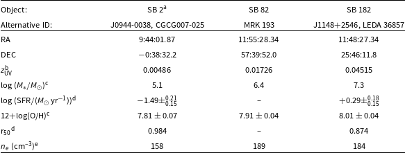
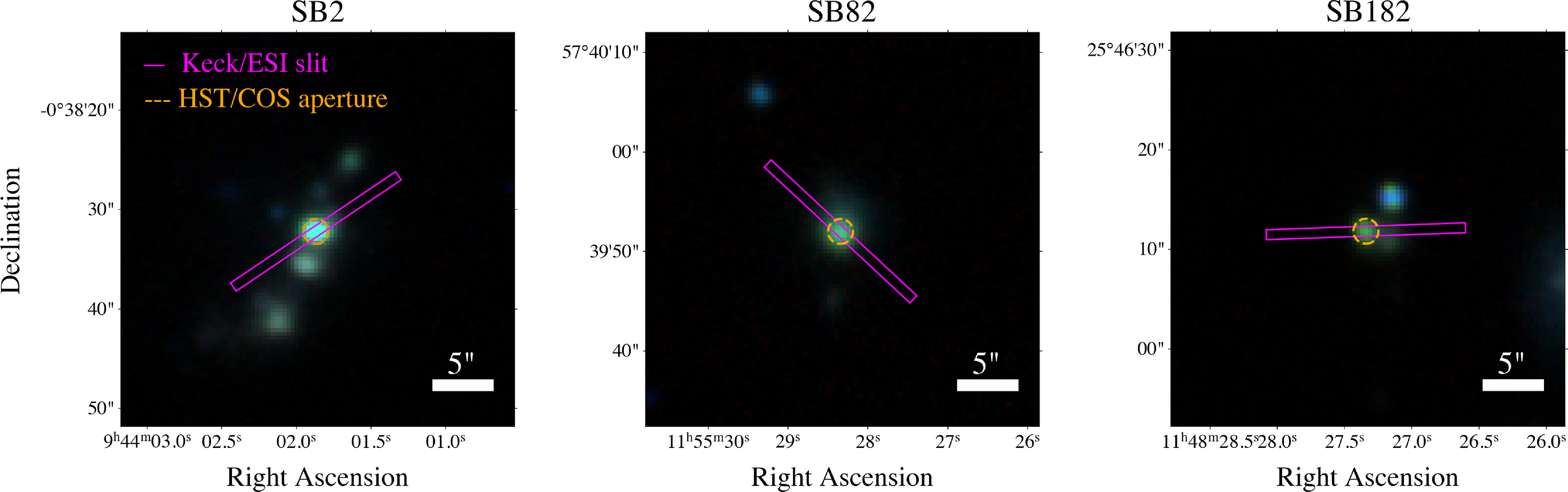


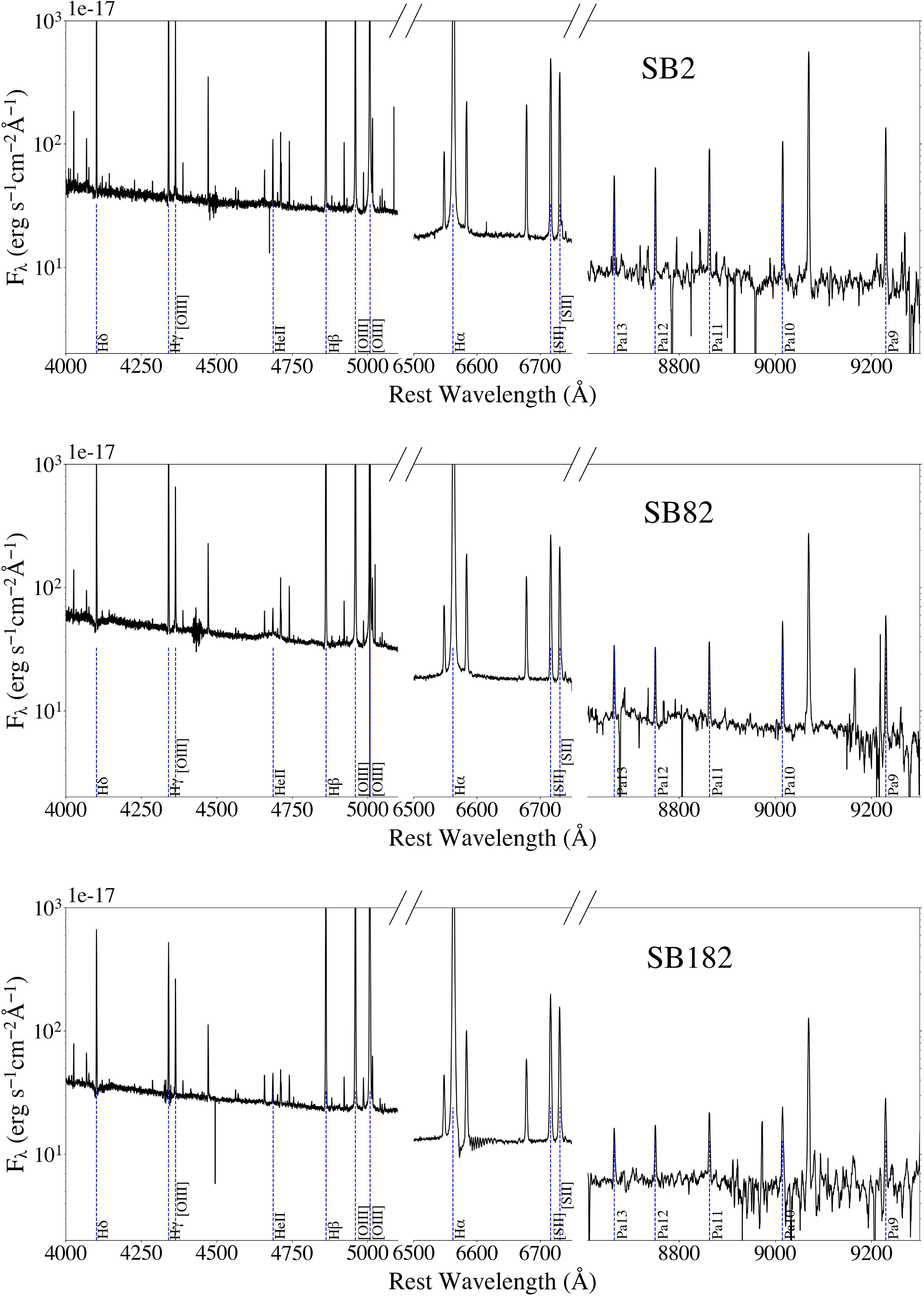

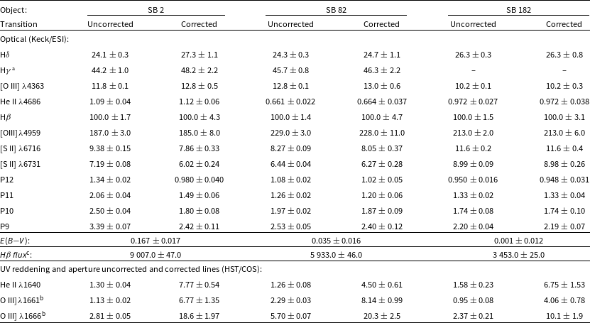

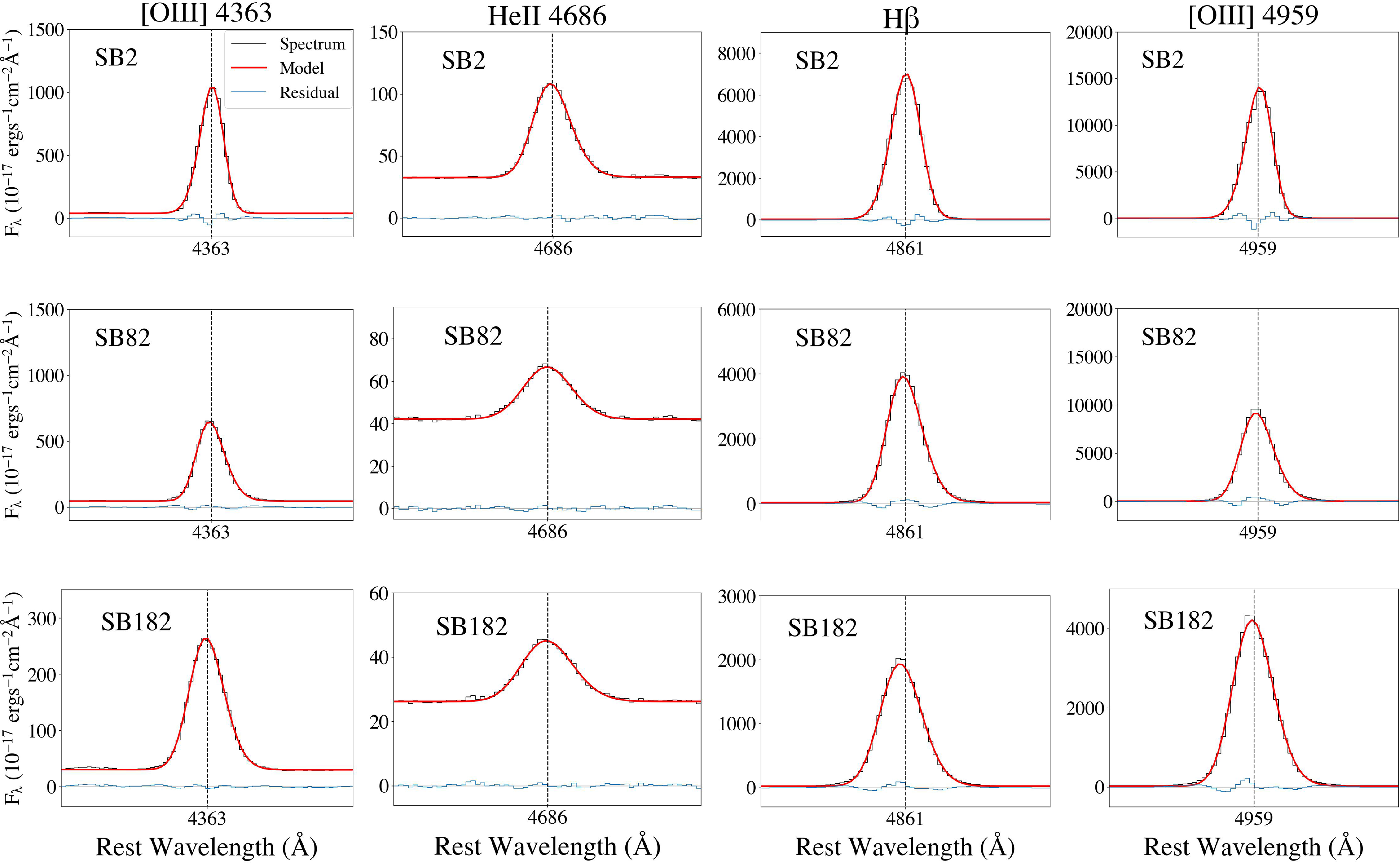


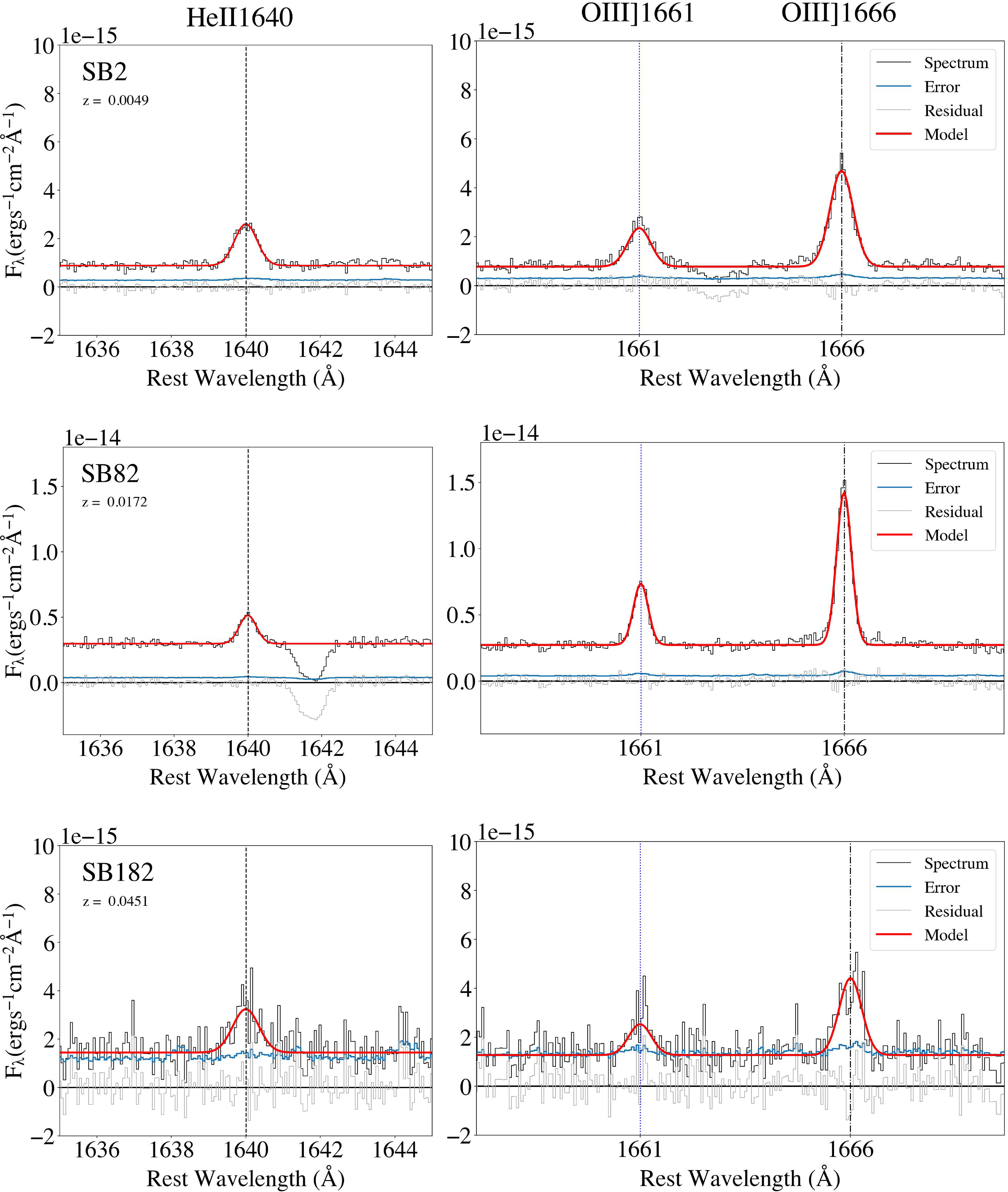


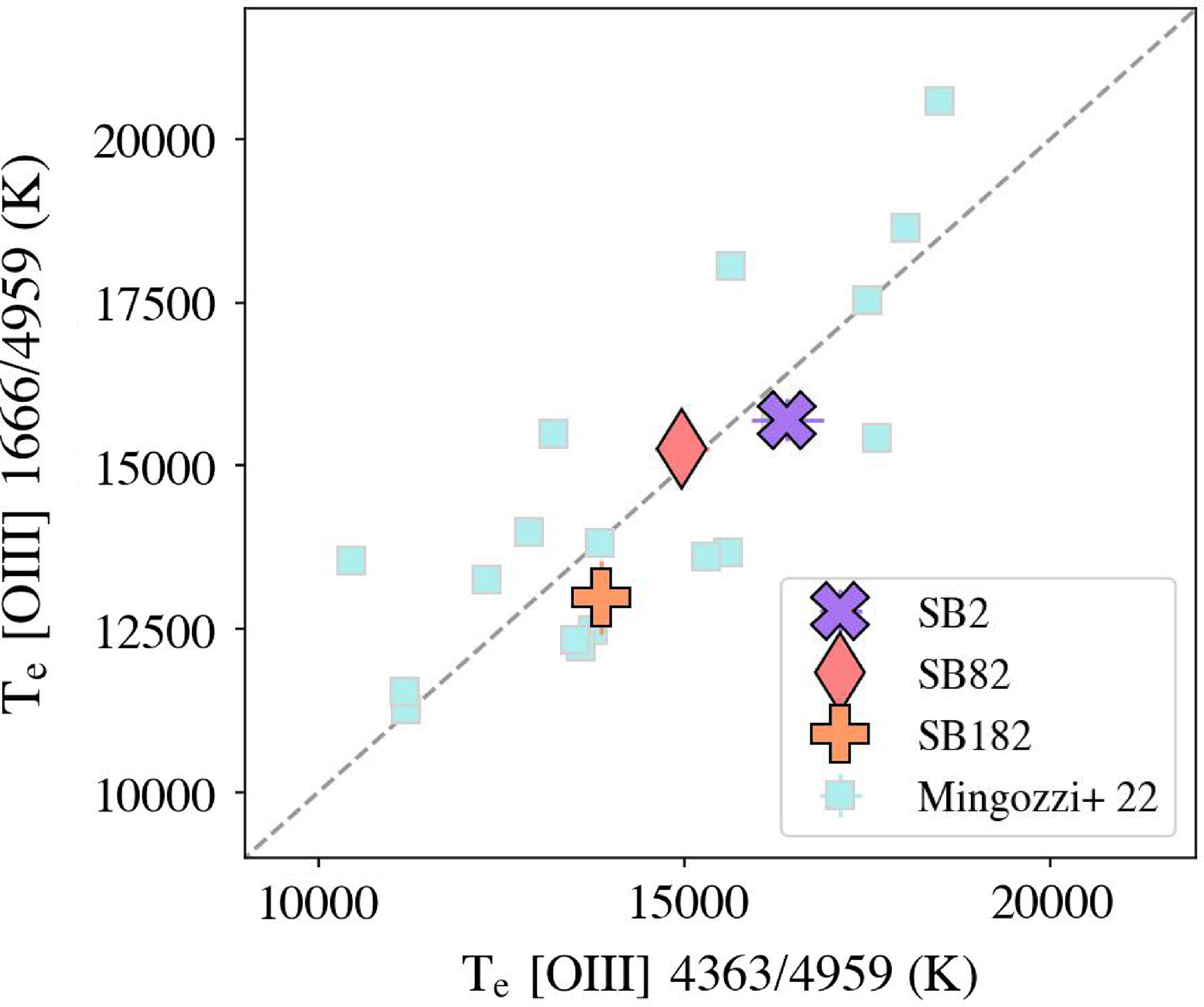


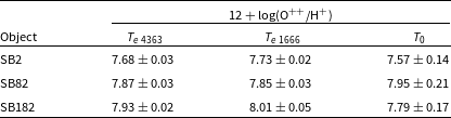


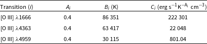


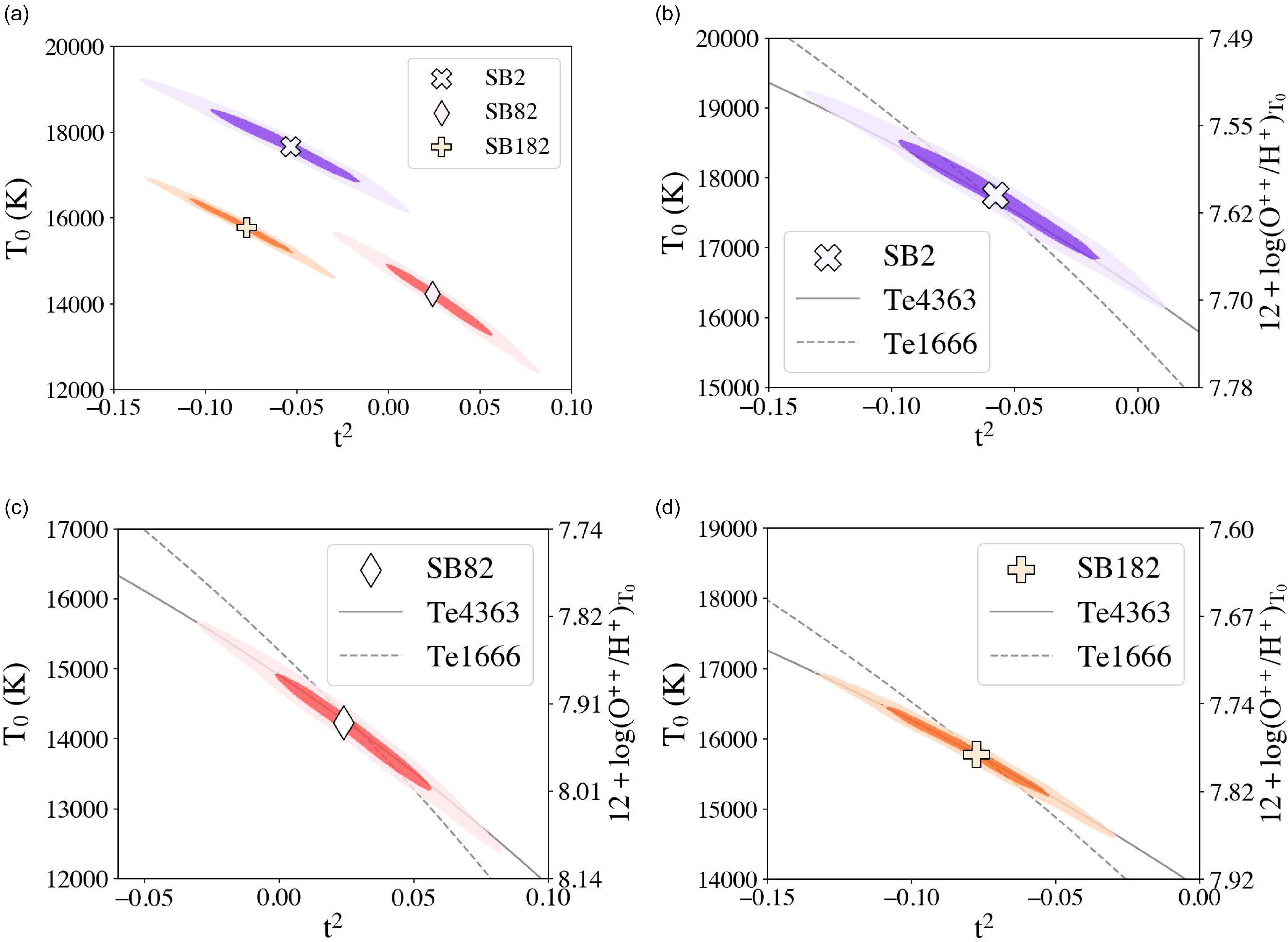


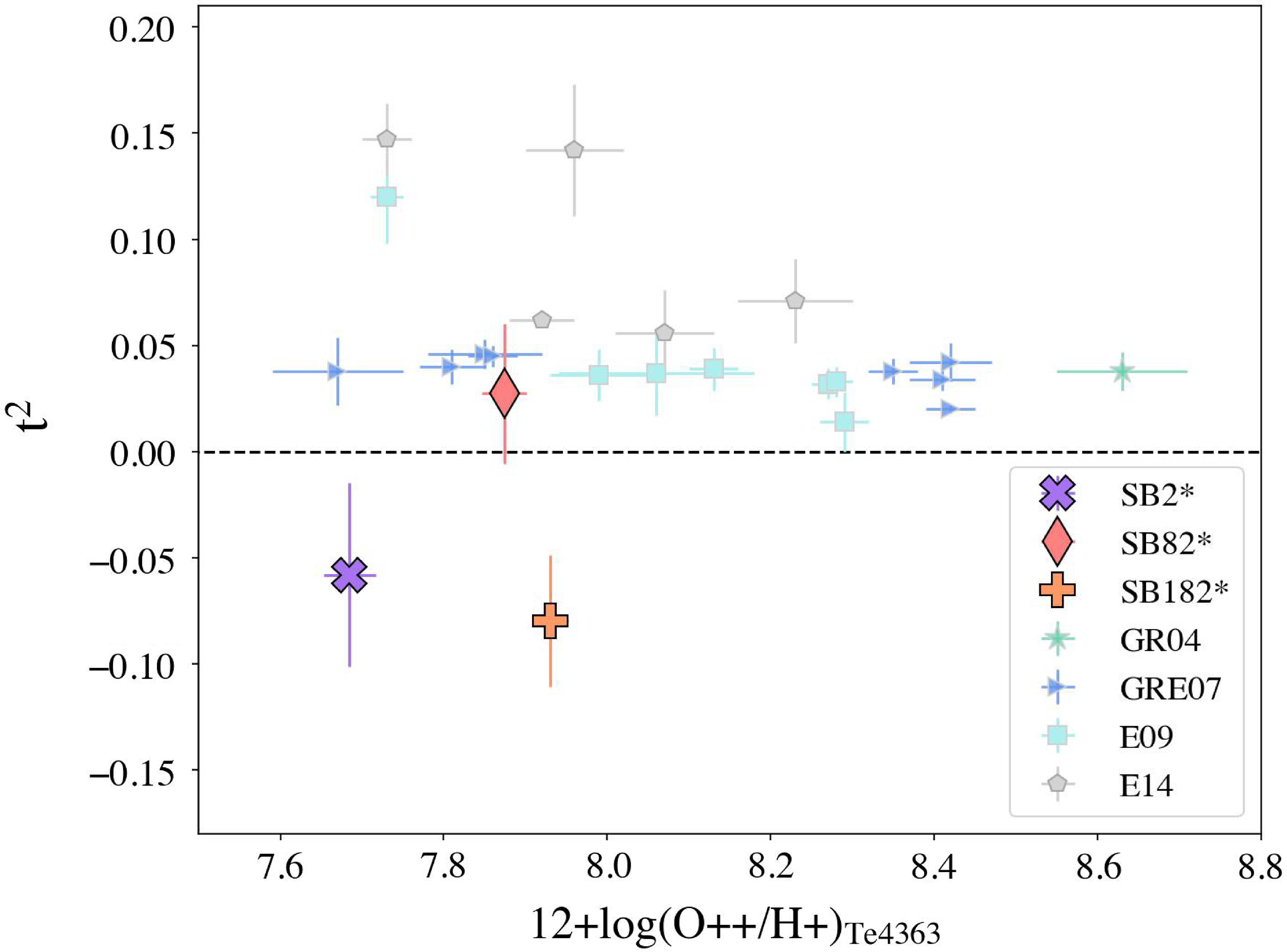


 Open access