Model description

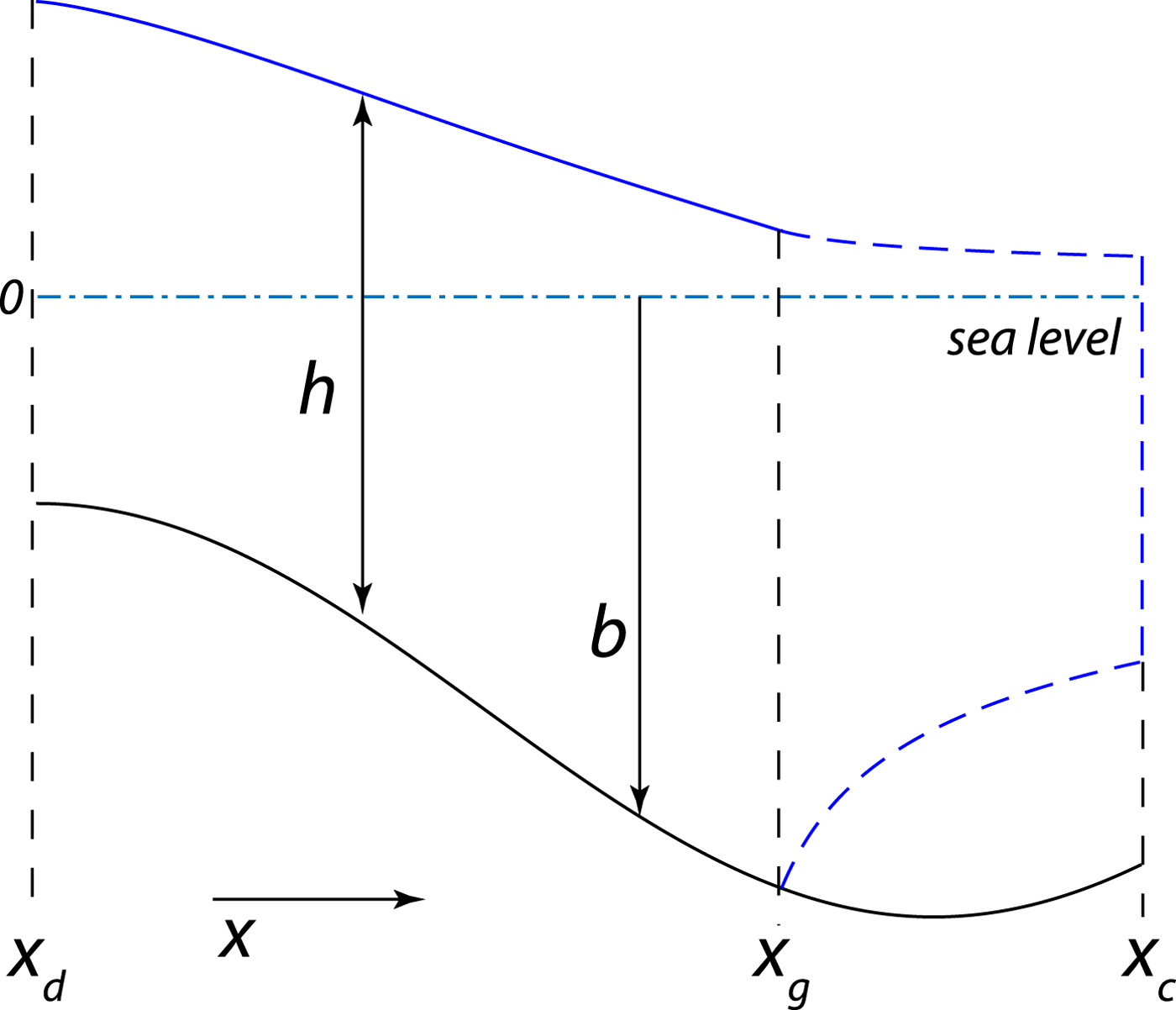
We consider an unconfined ice stream that flows into an unconfined ice shelf (Fig. 2) and use the model formulation of Schoof (Reference Schoof2007b), which we briefly describe below. Under assumptions of negligible vertical shear appropriate for ice stream and ice shelf flow (MacAyeal, Reference MacAyeal1989), the vertically integrated momentum balance is

(1a)$$ \eqalign{& 2\left( {A^{-(1/n)}h{\left| {u_x} \right|}^{(1/n)-1}u_x} \right)_x-\tau _{\rm b}-\rho gh\left( {h + b} \right)_x = 0, \cr & \quad x_d \le x \le x_j,} $ $$

(1b)$$ 2\left(A^{-({1}/{n})}h\left\vert u_x\right\vert ^{({1}/{n})-1}u_x\right)_x -\rho g^\prime hh_x=0, \quad x_j\leq x\leq x_c, $$

where u(x) is the depth-averaged ice velocity, h(x) ice thickness, b(x) is the bed elevation (negative below sea level and positive above sea level), A ^−1/n is the ice stiffness parameter (assumed to be constant), n is an exponent of Glen's flow law, g is the acceleration due to gravity, τ_b is basal shear, g′ is the reduced gravity defined as

(2)$$ g^\prime=\delta g $$

where

(3)$$ \delta = {\rho_{\rm w}-\rho \over \rho_{\rm w}} $$

is the buoyancy parameter, ρ and ρ _w are the densities of ice and water, respectively, x _d is the location of the ice divide (assumed to be x _d = 0), x _c is the location of the calving front and x _j is the location of the junction between the ice stream and ice shelf. In the absence of a universal ‘sliding law’ – a relationship between shear at the ice/bed interface and characteristics of ice and bed – several formulations are commonly used. Throughout the derivations presented below we adopt a formulation used by Schoof (Reference Schoof2007b)

(4)$$ \tau_{\rm b}=C\left\vert u\right\vert ^{m-1}u, $$

where C and m are constant parameters. The first term in (1a) is the divergence of the extensional, or longitudinal stress, τ_x, the second term is the basal shear, τ_b, and the final terms in the both equations are the driving stress, τ_d.

Fig. 2.

Model geometry: b – bed elevation (b <0), h – ice thickness, x _d – the ice divide location, x _g – the grounding line location; x _c – the calving front location.

The mass balance is

(5)$$ h_{\rm t}+\left(uh\right)_x =\left\{ \matrix{ \dot a & 0\leq x\leq x_{\rm j} \cr \dot m & x_{\rm j}< x\leq x_{\rm c},} \right. $$

where $\dot a$ and $\dot m$ are the net accumulation/ablation (positive for accumulation) rates of the ice stream and ice shelf, respectively. (The discontinuity at the junction x _j is due to the fact that basal ablation by the ocean is possibly discontinuous across the junction.)

The boundary conditions are

(6a)$$ (h+b)_x =0,\quad u=0, \quad x=0 $$

(6b)$$ 2 A^{-({1}/{n})}h\left\vert u_x\right\vert ^{({1}/{n})-1}u_x={1 \over 2}\rho g^\prime h^2, \quad x=x_{\rm c}. $$

The condition at the calving front, x _c, requires the longitudinal stress in the ice to balance the pressure deficit at the front. The conditions at the divide, x _d, are statements that there is no driving stress there, and that no flow enters or leaves the domain from the left. These are the natural conditions to describe a divide. A detailed treatment near the divide in fact requires the solution of a full-Stokes problem (Fowler, Reference Fowler1992). However, the primary concern of this paper is not the detailed behavior near the divide, and we will use (1)–(6), as a sufficient description.

At the junction, x _j continuity conditions have to be prescribed. The number of conditions is determined by the number of the boundary conditions for the ice stream and the ice shelf.

(7a)$$ u_{{\rm stream}}(x_{\rm j})=u_{{\rm shelf}}(x_{\rm j}) $$

(7b)$$ h_{{\rm stream}}(x_{\rm j})=h_{{\rm shelf}}(x_{\rm j}) $$

(7c)$$ \tau_{{\rm stream}}(x_{\rm j})=\tau_{{\rm shelf}}(x_{\rm j}). $$

The problems (1)–(7) provide solutions for any given location of the junction x _j. However, the solution h(x _j) must in addition satisfy the flotation condition

(8)$$ h(x_{\rm j}) = - {\rho_{\rm w} \over \rho} b(x_{\rm j}). $$

The grounding line location x _g is then determined as the root of this equation in x _j. We will use the symbols h _g, u _g and τ_g to mean ice thickness, velocity and the longitudinal stress at the grounding line.

Additionally, the following inequalities have to be satisfied

(9a)$$ h(x) \gt -{\rho_{\rm w} \over \rho}b(x), \quad 0 \lt x \lt x_{\rm g}, $$

(9b)$$ h(x)\leq - {\rho_{\rm w} \over \rho}b(x), \quad x_{\rm g}\leq x \lt x_{\rm c}. $$

These conditions reflect the fact that the ice stream is grounded and the ice shelf is floating. Similar to all previous studies of unconfined ice shelves (e.g., MacAyeal and Barcilon, Reference MacAyeal and Barcilon1988; Schoof, Reference Schoof2007b) we integrate the momentum balance of the ice shelf (1b), and using the boundary condition at the calving front, x _c, (6b) and the continuity conditions at the grounding line (7), and reduce the problem to the ice stream part only, with the boundary conditions at the grounding line – the flotation condition (8) and the stress condition

(10)$$ 2 A^{-({1}/{n})}h\left\vert u_x\right\vert ^{({1}/{n})-1}u_x={1 \over 2}\rho g^\prime h^2, \quad x=x_{\rm g}. $$

The model (1)–(10) is identical to one used by Schoof (Reference Schoof2007b).

In what follows we use precise numerical solutions of (1)–(10) to compare with approximate asymptotic expressions, and describe them as ‘exact’, acknowledging their numerical origin. To obtain the ‘exact’ solutions, we use the finite-element solver Comsol™, (COMSOL, 2018), whose accuracy is well-established (e.g. Schäfer and Turek, Reference Schäfer, Turek and Hirschel1996).

We now proceed to non-dimensionalize (1)–(10) using as characteristic scales the bathymetry of a continental shelf [b], the length of an ice steam [x] and its velocity [u]. In terms of these

(11)$$ [h]=[b], \quad [\dot a] ={[b][u] \over [x]}, \quad [t] = {[x] \over [u]}. $$

With the two non-dimensional parameters

(12a)$$ \varepsilon= {2A^{-({1}/{n})}[u]^{1/n} \over \rho g[h][x]^{1/n}} $$

(12b)$$ \gamma = {[C][u]^m[x] \over \rho g[h]^2}, $$

relating to deformation and sliding, respectively, the non-dimensional momentum balance and mass balance become

(13)$$ \varepsilon\left(h\left\vert u_x\right\vert ^{({1}/{n})-1}u_x\right)_x - \gamma\left\vert u\right\vert ^{m-1}u-h(h+b)_x=0, \quad 0\leq x\leq x_{\rm g}, \quad h\leq- {b \over 1-\delta} $$

and

(14)$$ h_{\rm t}+\left(uh\right)_x = \dot a, \quad 0\leq x\leq x_{\rm g}. $$

The non-dimensional boundary conditions at x = 0 and x = x _g are

(15a)$$ (h+b)_x =0,\quad u=0, \quad x=0 $$

(15b)$$ \varepsilon h\left\vert u_x\right\vert ^{({1}/{n})-1}u_x={1 \over 2}\delta h^2, \quad x=x_{\rm g}, $$

(15c)$$ h=-{b(x) \over 1-\delta} \quad x=x_{\rm g}. $$

The inequality constraint (9) is

(16)$$ h(x) \gt -{b(x) \over 1-\delta}, \quad 0 \lt x \lt x_{\rm g}. $$

The non-dimensional problem (13)–(16) has three non-dimensional parameters: ε, expression (12a), γ, expression (12b) and δ, expression (3). Their magnitudes are determined by the characteristic scales of the problem. The buoyancy parameter δ, defined by (3), is determined by the values of densities of ice, ρ = 917 kg m⁻³, and sea-water, ρ _w ≈1020 kg m⁻³, which results in δ ≈ 0.1. To determine the value of ε, we take as the characteristic scales for the present-day Antarctic ice streams to be D = 1000 m, L = 500 km and V = 500 m a⁻¹ (Fretwell and others, Reference Fretwell2013) together with the ice rheological parameters n = 3 and A = 1.35 · 10⁻²⁵ Pa⁻³ s⁻¹ (that corresponds to the ice temperature T = −20°C). These then provide the value for parameter ε is ~1.4·10⁻² ≪1.

The choice of γ is not determined by direct observations, because the basal shear, τ_b, is not directly observed, and must be inferred from the surface observations, e.g., by means of inversion techniques from surface observations (e.g. MacAyeal, Reference MacAyeal1992; Sergienko and others, Reference Sergienko, Bindschadler, Vornberger and MacAyeal2008; Sergienko and Hindmarsh, Reference Sergienko and Hindmarsh2013). We obtain a value of C based on the results of limited direct observations of the basal conditions (e.g., Engelhardt and others, Reference Engelhardt, Humphrey, Kamb and Fahnestock1990) and results of inverse modeling studies (e.g, MacAyeal, Reference MacAyeal1992; MacAyeal and others, Reference MacAyeal, Bindschadler and Scambos1995; Joughin and others, Reference Joughin, MacAyeal and Tulaczyk2004; Sergienko and others, Reference Sergienko, Creyts and Hindmarsh2014) indicating that basal shear under ice streams has small magnitudes. For instance, using Stokes' equations as a forward model, Sergienko and others (Reference Sergienko, Creyts and Hindmarsh2014) find that the inferred values of the basal shear in the trunks of MacAyeal and Bindschadler ice streams is ~0.5–5 kPa. Consequently, characteristic scales of the sliding parameter C are 2·10⁴–2·10⁵ Pa m^−1/3 s^1/3, and according to (12b), γ ~2.8·10⁻² – 2.8 ·10⁻¹.

We seek to provide an approximate solution of the problem (13)–(16), and this requires us to assign relative orders or the three parameters, ε, γ and δ.

As shown above ε and γ are naturally regarded as small, and we take ε ~ γ ~ o(1); but the choice of the order of δ is open to us. One choice is to follow Schoof (Reference Schoof2007b) and take δ as O(1). As we noted in section ‘Introduction’, this leads, as a consequence of the resulting imbalance of terms in the boundary condition (15b), to suppose the existence of a boundary layer close to x _g in which the longitudinal and basal stress terms in the momentum balance (13) are of the same order as the driving stress (Schoof, Reference Schoof2007b; Tsai and others, Reference Tsai, Stewart and Thompson2015). The alternative is to take δ as a small parameter, and, indeed, with our choice of scales δ is closer to ε than to unity. We accordingly take δ ~ ε. This will remove the need for a boundary layer at the junction. The effectiveness of this assignment may be judged from the numerical results we describe later.

The problem can then be reduced to one in which δ is the sole parameter through rescaling in the following fashion using the parameter ε/δ:

(17)$$ h=\left({\varepsilon \over \delta}\right)^\alpha H,\quad b=\left({\varepsilon \over \delta}\right)^\alpha B,\quad u=\left({\varepsilon \over \delta}\right)^\beta U,\quad x=\left({\varepsilon \over \delta}\right)^\kappa X,\quad t=\left({\varepsilon \over \delta}\right)^\sigma T. $$

Substituting these expressions into the momentum balance (13), mass balance (14) and the boundary conditions (15), balancing the first and second terms $\displaystyle {(1+\alpha -\kappa +(({\beta -\kappa })/{n})=1+m\beta )}$ in the momentum balance, all terms in the mass balance (α − σ = α + β − κ = 0), and the both sides in the stress (15b) condition at x _g (1 + α + ((β − κ)/n) = 2α) we get

(18)$$ \alpha=\sigma={n \over n+1},\quad \beta=-{1 \over (m+1)(n+1)}\left(=-{n \over n+1}\right),\quad \kappa={n(m+1)-1 \over (m+1)(n+1)}\left(=0\right), $$

where expressions in parentheses are for the case of γ = 0, so that, in this case, x does not need rescaling. The rescaled problem becomes

(19a)$$ \delta\left(H\left\vert U_X\right\vert ^{({1}/{n})-1}U_X\right)_X -\delta \Gamma\left\vert U\right\vert^{m-1}U-H(H+B)_X=0, $$

(19b)$$ H_T+(UH)_X=\dot a $$

(19c)$$ (H+B)_X =0,\quad U=0, \quad X=0 $$

(19d)$$ H\left\vert U_X\right\vert ^{({1}/{n})-1}U_X={1 \over 2} H^2,\quad X=X_{\rm g} $$

(19e)$$ H=-{B \over 1-\delta} \quad X=X_{\rm g} $$

(19f)$$ H \gt -{B \over 1-\delta},\quad 0<X<X_{\rm g} $$

where $\displaystyle {\Gamma ={\gamma }/{\varepsilon }}$ and the subscripts X and T are derivatives with respect to the coordinate X and time T. In contrast to the original problem (13)–(16) a small parameter δ appears only in the momentum balance (19a). This reduction, which was introduced by Schoof (Reference Schoof2007b, Appendix A) in connection with the corresponding problem in which the basal stress is of the same order as the driving stress, is exact: the solution for any pair of values of ε and δ may be obtained from the solution of the problem (19) through the scale assignment (17). However if, as we do here, one seeks an approximate solution of the problem (19) as a perturbation series expansion in the small parameter δ, one must formally assign δ ~ ε if the other terms in (19) are to be O(1).

To illustrate how different scales of basal shear affect the steady-state configurations we solve the problem (1)–(9) numerically (the details of numerical solver and used parameters are described in Appendix A) with two different values of the sliding parameter C. In the first experiment we use the same value as used by Schoof (Reference Schoof2007b) C = 7.6 · 10⁶ Pa m^−1/3 s^1/3; in the second experiment, we use the value of C three orders of magnitude smaller C = 7.6 · 10³ Pa m^−1/3 s^1/3. The computed ice-stream geometry and the momentum balance components for the two cases are markedly different (Fig. 3). In the case of a large value of the sliding coefficient, ice thickness is significantly larger in the interior than the magnitude of the bed elevation throughout the ice stream, and also than the ice thickness in the immediate vicinity of the grounding line. Consequently, the surface gradients are large in the vicinity of the grounding line (Fig. 3a). In contrast, in the case of low value of C, surface elevation neither varies substantially through the length of the ice stream nor in the immediate vicinity of the grounding line (Fig. 3d). Also, the ice thickness has the same order of magnitude as bed elevation, and for the chosen bed geometry, it is larger at the grounding line than in the interior of the ice stream.

Fig. 3.

Surface elevation and components of the momentum balance for a high C = 7.6 · 10⁶ Pa m^−1/3 s^1/3 (panels (a)–(c)) and low C = 7.6 · 10³ Pa m^−1/3 s^1/3 (panels (d)–(e)) values of the sliding coefficient. Panels (a) and (d) surface (s) and bed (b) elevation (m), arrows show the ice-flow direction; (b), (c) and (e) components of the momentum balance, τ_x, τ_b and τ_d (kPa); insets in panel (b) show locations of a zoom shown in panel (c) τ_x for C = 7.6 · 10⁶ Pa m^−1/3 s^1/3. The simulation parameters are the following: bed elevation b(x) = b ₀ + b _acos (πx/L), with b ₀ = −500 m, b _a = 250, and L=500 km; ice stiffness parameter A = 1.35 · 10⁻²⁵ Pa⁻³ s⁻¹ (corresponds to T _ice ≈ −20^°C); and accumulation rate $\dot a=0.94$ m a⁻¹.

The momentum balance in the case of large C (Fig. 3b) is predominantly between the driving and basal stresses. These are of the order of 100–200 kPa throughout the length of the ice stream, and achieve their maximum at the grounding line. Although the divergence of the longitudinal stress increases near the grounding line (Fig. 3c), its magnitude remains significantly (two orders) smaller than the magnitudes of the driving and basal stresses. In the case of low C (Fig. 3e), the driving and basal stresses are much smaller than in the case of large C (less than 1 kPa), and the divergence of the longitudinal stress is of the same order as the basal shear (Fig. 3e), in line with the conclusions of MacAyeal (Reference MacAyeal1989) who found that ‘…basal drag and horizontal deviatoric stress gradients can contribute equally in balancing gravitational driving stress.’ These results suggest that the two regimes of high and low basal and driving stresses are very different; they also suggest that the power-law sliding law is capable of producing low surface gradients and low driving stress not only in the vicinity of the grounding line, but through the length of the ice stream, if the sliding coefficient C is small.

Steady states

In this section, we investigate steady solutions to (19) by setting H _T in (19b) to zero. We treat δ as a small parameter and seek a solution as series expansion in δ, i.e.

(20a)$$ H\sim H_0+\delta H_1+\delta^2 H_2 +\cdots $$

(20b)$$ U\sim U_0+\delta U_1+\delta^2 U_2 +\cdots $$

where the coefficients of powers of δ are supposed of O(1). Substituting H and U into the momentum-balance Eqn (19a), the mass-balance equation

(21)$$ (UH)_X=\dot a $$

and the boundary conditions (19c)–(19e), and equating the coefficients of each power of δ leads to various orders approximations of the problem (19a), (21) and (19c)–(19e). Detailed descriptions of the zeroth- and first-order solutions are provided in Appendix A. In this section we provide a brief summary.

The zeroth-order problem is

(22a)$$ H_0(H_0+B)_X=0 $$

(22b)$$ (U_0H_0)_X=\dot a $$

(22c)$$ U_0=0, \quad X=0 $$

(22d)$$ (H_0+B)_X=0, \quad X=0 $$

(22e)$$ H_0\left\vert U_{0X}\right\vert ^{({1}/{n})-1}U_{0X}={1 \over 2}H_0^2,\quad X=X_{\rm g} $$

(22f)$$ H_0=-B, \quad X=X_{\rm g}. $$

Its solutions, H ₀ and U ₀, are determined from (22a) together with (22f), and (22d)

(23a)$$ H_0(X)=-B(X) $$

(23b)$$ U_0(X)={\int_0^X\dot adx \over H_0(X)}={Q \over H_0}, $$

where $Q=\int _0^X \dot a dx$ is ice flux.

Expression (23a) describes a solution in which the stream is neutrally buoyant: the thickness equals the bed depth and the surface elevation is zero. It provides no description of the roles of the divergence of the longitudinal stress and the basal shear stress in determining the position of the grounding line, for which we need to determine the first-order solutions. The zeroth-order solution does, however, provide an important insight. Using (23), the stress condition (22e) can be written as

(24)$$ QB_{X}-\dot aB=\left({1 \over 2}\right)^n\left\vert B\right\vert ^{n+2},\ X=X_g, $$

which provides an expression for the grounding flux. Q(X _g) is not a function of B(X _g) alone, as is the case with a high basal shear stress (Schoof, Reference Schoof2007b), but depends in addition on the basal gradient at the grounding line. This arises because, at this order, the surface is flat, and it is the basal gradient, rather than the surface gradient, that accounts for the ice thickness gradient. We will return to the implications of this observation having first obtained the first-order solutions.

The first-order problem is

(25a)$$ H_{1X}={1 \over H_0}\left[\left(H_0\left\vert U_{0X}\right\vert ^{({1}/{n})-1}U_{0X}\right)_X -\Gamma\left\vert U_0\right\vert ^{m-1}U_0\right] $$

(25b)$$ (U_1H_0+U_0H_1)_X=0 $$

(25c)$$ U_1=0, \quad X=0 $$

(25d)$$ H_{1X}=0, \quad X=0 $$

(25e)$$ H_1\left\vert U_{0X}\right\vert ^{({1}/{n})-1}U_{0X}+{1 \over n}H_0\left\vert U_{0X}\right\vert ^{({1}/{n})-1}U_{1X}=H_1H_0, \quad X=X_{\rm g} $$

(25f)$$ H_1=-B, \quad X=X_{\rm g}. $$

All the components of the first-order expressions are determined from the zeroth-order solutions U ₀ and H ₀ (23). Substitution of these solutions and their derivatives into (25a) gives

(26)$$ \eqalign{ H_{1X} = &{\vert B\vert ^{-(({n+2})/{n})} \over n}\left\vert QB_{X}-\dot aB\right\vert ^{({1}/{n})-1}\big[(2-n)B_{X}(QB_{X}-\dot aB) -\cr &B(QB_{XX}-B\dot a_X)\big]-\Gamma{Q^m \over \vert B\vert ^{m+1}}.} $$

This expression has two terms that are determined by bed properties – its geometry (the first term) and basal shear (the second term). The first term, which includes bed elevation B (note that B is a negative quantity), its slope B _X, and curvature B _XX, can be regarded as a form drag, which is the resistance to ice flow that arises due to the shape of the bed (e.g. Schoof, Reference Schoof2002a). The last term of (26) is the basal shear expressed in terms of ice flux $\displaystyle {Q=U_0H_0}$. The fact that the basal shear is an additive term suggests that in the low basal and driving stress regimes, ice flow is less sensitive to a specific form of basal shear (‘sliding law’) as long as its magnitude is low.

In general (26) is not compatible with (25d), suggesting the presence of a boundary layer at the divide at first order. However, as we have already noted, our interest is not in the details at the divide, and we therefore impose a further constraint that $(n-2)B_X\dot a+ B\dot a_X=0$ at X=0. This is satisfied if, e.g., the bed elevation and accumulation rate have no gradients at the divide, i.e., B _X(X = 0) = 0 and $\dot a_X(X=0)=0$.

Taking into account the boundary condition (25c), a solution of (25b) is

(27)$$ U_{1}=-U_0{H_1 \over H_0}. $$

H ₁ is determined by integrating (26) using the flotation condition (25f).

Except for the case B = const, which is of limited interest, (26) cannot be integrated analytically. H ₁ is ice surface elevation to leading order. It is determined by the integral of expression (26) that itself depends on only the local bed geometry and basal shear. The surface elevation is a non-local function of these bed properties, and depends on their integral effects through the length of the ice stream.

At this point the zeroth- and first-order solutions are determined for any given location of the junction between an ice stream and ice shelf, but we have yet to determine the position of the grounding line X _g. For this purpose we use the remaining stress boundary condition (19d), and determine the grounding line location through the simultaneous solution of this condition and the momentum and mass-balance solutions in the interior of ice stream.

Combining the zeroth- and first-order stress conditions (22e) and (25e), the flotation conditions, (22f) and (25f), the zeroth-order solutions (23) and the first-order solution for U ₁ (27), the stress condition (19d) becomes

(28)$$ \eqalign{ \vert QB_{X}&-\dot aB\vert ^{({1}/{n})-1}\left[\left(1-{\delta \over n}\right)\left(QB_{X}-\dot aB\right)-{\delta \over n}Q\left(H_{1X}+B_{X}\right)\right] =\cr & {1+\delta \over 2}\left\vert B\right\vert ^{(({n+2})/{n})}, \quad X=X_{\rm g}.} $$

where H _1X is given by (26) evaluated at X = X _g. Values of X _g are determined as the roots of (28). It is possible that the choices of the functions B and $\dot a$ can produce zero, one or more steady-state locations of the grounding line.

Comparing (28) and (24) one can see that acknowledging the role of the basal shear stress and the form drag further increases the parameters on which the flux at the ground line depends to include the basal curvature and the basal sliding coefficient Γ. The dimensional form of (28) is

(29)$$ \eqalign {&\left\vert qb_{x}-\dot ab\right\vert ^{(1-n)/{n}} \left[ \left( 1-{\delta \over n} \right) \left(qb_{x}-\dot ab\right) - {\delta \over n} q \left( h_{1x}+b_{x}\right) \right] = \cr & \quad \rho g^\prime A^{({1}/{n})} \vert b\vert ^{({n+2})/{n}} {1+\delta \over 4}, \quad x=x_{\rm g},} $$

where

(30)$$\eqalign{ h_{1x}&={1 \over \rho g^\prime \vert b\vert }\left\{{2A^{-({1}/{n})} \over n\vert b\vert ^{2 \over n}}\left\vert qb_{x}-\dot ab\right\vert ^{({1}/{n})-1}\big[(2-n)b_{x}(qb_{x}-\dot ab)-\right. \cr & \left. \quad b(qb_{xx}-b\dot a_x)\big]-C\left({q \over \vert b\vert }\right)^m\right\},} $$

where b(x) <0.

Expression (29) may be compared with the relationship derived for unconfined configurations in a regime with a large magnitude basal shear (Schoof, Reference Schoof2007b)

(31)$$ q=\left({A\left(\rho g\right)^{n+1}\delta^n \over 4^nC}\right)^{{1}/({m+1})}\left({\vert b\vert \over 1-\delta}\right)^{({m+n+3})/{m+1}}, \quad x=x_{\rm g}, $$

where we have applied the flotation condition on the RHS of (31) so to make it comparable with (29). Equation (29) is considerably more complex than (31), and in particular it depends upon the bed shape, and the accumulation rate and its gradient at the grounding line, in addition to the bed elevation itself. According to these, ice streams with the same bed depth at the grounding line can have different fluxes and vice versa; and the relationship can be a multivalued function. Expression (28) results in an ice flux with a finite magnitude even when the basal shear is zero, in contrast to the infinite flux which is the consequence of (31) as C →0.

Comparison of approximate and ‘exact’ solutions

To assess the behaviors of the zeroth- and first-order solutions, and to compare these with the ‘exact’ solutions, we compute the grounding line position, and the relationship between flux and thickness at the grounding line, for the sinusoidal bed illustrated in Figure 4a, as the accumulation rate is varied. The grounding line positions for the case of the sliding parameter C=0 are shown in Figure 4a, the relationships between ice flux and thickness for various values of the sliding parameter C in Figures 4b and 4c. As Figure 4b shows, the relationship between flux and thickness is not a simple, monotonic curve. In this case, for a given flux, steady states can be found at two thicknesses, or for a given thickness, steady states can be found for two values of flux. As C increases, the relative importance of form drag and basal shear changes, and the difference between multiple values decreases. Figures 4a and 4b show solutions obtained from the zeroth- and first-order solutions. The multivalued behavior is qualitatively captured in the zeroth-order solution (black asterisks), although the addition of the role of form drag, which is accounted for when the first-order solution is included and C = 0, and the basal shear stress as C increases are quantitatively different. The quantitative difference is apparent too in the grounding line locations. Figure 4a shows three examples of the grounding line positions computed from the zeroth-order expression (24) (black asterisks labeled ‘1–3’). These positions are substantially different from the ‘exact’ positions and approximate ones computed using the first-order solutions (filled blue circles and diamonds labeled ‘1–3’).

Fig. 4.

Conditions at the grounding line. (a) The grounding line position for sliding parameter C=0 and discreet values of the accumulation rate $\dot a$; (b) and (c) the relationship between ice flux and ice thickness computed for various values of the accumulation rate $\dot a$ and sliding parameter C. The values of $\dot a$ are discretely chosen, ranging from 0.18 to 39.8 m a⁻¹. The size of symbols in panels (a) and (b) correspond to the values of $\dot a$. In panels (a) and (b) circles are ‘exact’ computations, diamonds are the roots of expression (29), asterisks are the roots of the zero-order expression (24). In panel (a) black asterisks with black labels ‘1–3’ are three examples of the roots of the zeroth-order expression (24); filled symbols with blue labels ‘1–3’ are the roots of expression (29) with the same values of $\dot a$ as those denoted by black asterisks. The labels ‘1–3’ in panel (b) correspond to the labeled grounding line locations in panel (a). Circles in panel (c) are ‘exact’ solutions and solid lines are the boundary layer relationship (31) derived by Schoof (Reference Schoof2007b). Notice logarithmic scale on the vertical axis on panel (c). The bed elevation b(x) has the same analytic form and stiffness parameter A has the same value as those in Figure 3. In all experiments the ice flow is from left to right.

Figures 4a and 4b also include a comparison with the ‘exact’ solutions (denoted by circles). These show a good agreement between the ‘exact’ results and expression (29). This close coincidence indicates that the scale assignment of δ provides a description that closely resembles the actual dynamics. That accurate solutions require a solution to O(δ) reflects the fact that the value of δ is 0.1. This numerical value is material, in that accurate solutions then need to account for the form drag, and the basal shear if it is present. In detail, there are values of accumulation rate for which the zeroth- and first-order solutions do not provide a solution for a steady-state grounding line, although the ‘exact’ solutions do provide one. These are indicated by fewer diamond and asterisk symbols indicating the approximate and zero-order solutions compared to the circle symbols indicating the ‘exact’ solutions in Figures 4a and 4b.

Figure 4c extends the range of 4b to allow a comparison for values of C of which the basal shear stress is much larger than the contribution of form drag. It shows that the effects of form drag are completely suppressed and the flux–thickness relationship follows expression (31) (purple line in Fig. 4c). On the other hand, for smaller values of C expression (31) (solid lines in Fig. 4c) consistently overestimates ice flux (and, as we have noted, results in infinity if the basal shear is zero). (Because (29) is not applicable for high values of C, in Figure 4c we have used ‘exact’ solutions for consistency.)

In circumstances where the basal shear is small, the surface slopes and driving stress are determined by the gradient of the longitudinal stress τ_x (the first term on the RHS of (25a) and (30)), which in turn is determined by the ice stiffness parameter A and spatial variability of the bed elevation. Gudmundsson (Reference Gudmundsson2003) and Sergienko (Reference Sergienko2012) show that the effects of the variability in bed elevation on ice flow increase as the basal shear decreases. Figure 5 illustrates the effects of form drag on ice-stream flow. It shows the analytical (blue curves in panels 5a–5b and 5d–5e) and ‘exact’ solutions (red curves in panels 5a–5b and 5d–5e) with the sliding parameter C=0 for two bed elevations that have the same slope, but one of which has low-amplitude long-period (more than 10 ice thicknesses) undulations $\displaystyle {b(x)=b_0+ b_xx+b_a \sin ({\pi x}/{L})}$ where b ₀ = −100 m, b _x = −0.0005, b _a = 5 m, and L=5 km (Figs 5a–5c) and whereas the second one does not $\displaystyle {b(x)=b_0+ b_xx}$, where b ₀ = −200 m, b _x = −0.0005 (Figs 5d–5f). The configurations of the two ice streams are significantly different: the grounding line position in the case of the bed with undulations is ~116 km upstream of the grounding line position in the case of the bed without undulations; the maximum ice flow speed is 26% slower in the former case than in the latter case; the maximum magnitude of the divergence of the longitudinal stress (and consequently driving stress) is more than two orders of magnitude larger in the former case than in the latter, although it is noticeable that the surface elevation in both cases is very similar. When the basal shear stress is low, the detailed shape of the bed has a strong influence on the location of the grounding line.

Fig. 5.

Effects of form drag. Steady-state configurations computed with C=0 for two bed elevation profiles: b(x) = b ₀ + b _x x + b _asin (πx/L) panels (a)–(c) and b(x) = b ₀ + b _x x panels (d)–(f). (a) and (d) profiles of surface and bed elevation, arrows show the ice-flow direction; (b) and (e) ice velocity; (c) and (f) the momentum-balance components. The terms of the momentum-balance (panels (c) and (f)) computed numerically. Note that panels (c) and (f) show − τ_d.

Linear stability analysis of steady states

The conclusion that a grounding line is unconditionally unstable if the bed slope is retrograde, due to Weertman (Reference Weertman1974) and given a more precise form by Schoof (2012), depends on the result (31) that the grounding line flux is a monotonically increasing function of the depth of the bed. However, as our results show, this result holds only when the basal shear and driving stress have large magnitudes. When the driving and basal shear stresses are small, the flux–thickness relationship (29) explicitly depends on the basal slope b _x and curvature b _xx, the accumulation rate $\dot a$ and its gradient $\dot a_x$, the basal shear stress, and the exponent n of the ice rheology (n >2 or n ≤2). Their various combinations could equally result in an increase or decrease in the ice flux with increase in ice thickness. One might anticipate that the stability of the grounding line position may exhibit a similar complexity.

To investigate the stability of the steady-state grounding line positions, we consider a time-variant problem with small deviations from a steady-state configuration, i.e.,

(32a)$$ H=H_{{\rm ss}}(X)+\sigma\tilde H(X,T), $$

(32b)$$ U=U_{{\rm ss}}(X)+\sigma\tilde U(X,T), $$

(32c)$$ X_{\rm g}=X_{{\rm gss}}+\sigma\tilde X_{\rm g}(T) $$

where σ is a small perturbation parameter and H _ss, U _ss and X _gss are the solutions of (19a), (21) and (19c)–(19e). Substituting these expressions into the momentum, mass-balance equations and the boundary conditions and collecting the terms of O(σ) yields the following perturbation problem

(33a)$$ \eqalign{\delta\left[\tilde H\left\vert U_{{\rm ss}X}\right\vert ^{({1}/{n})-1}U_{{\rm ss}X}+{1 \over n}H_{{\rm ss}}\left\vert U_{{\rm ss}X}\right\vert ^{({1}/{n})-1}\tilde U_X\right]_X- \cr \tilde H_XH_{{\rm ss}}-\tilde H\left(H_{{\rm ss}}+B\right)_X-m\delta\Gamma \left\vert U_{{\rm ss}}\right\vert ^{m-1}\tilde U=0 }$$

(33b)$$ \tilde H_T+\left(\tilde UH_{{\rm ss}}+\tilde HU_{{\rm ss}}\right)_X\;=0 $$

(33c)$$ \tilde H_X=\tilde U=0,\quad X=0 $$

$$ {1 \over n} H_{{\rm ss}}\left\vert U_{{\rm ss}X}\right\vert ^{({1}/{n})-1}\tilde U_X+\left (H_{{\rm ss}}\left\vert U_{{\rm ss}X}\right\vert ^{({1}/{n})-1}U_{{\rm ss}X}\right)_X\ \tilde X_{\rm g}=$$

(33d)$$ H_{{\rm ss}}\left(H_{{\rm ss}X}\tilde X_{\rm g}+{1 \over 2}\tilde H\right),\quad X=X_{{\rm gss}} $$

(33e)$$ \tilde H+H_{{\rm ss}X}\tilde X_{\rm g}=-{B_X \over 1-\delta}\tilde X_{\rm g},\quad X=X_{{\rm gss}}. $$

As in the previous section, we use the method of perturbation series expansion to construct to O(δ) solutions of (33). This is algebraically quite complex, and we give the details in Appendix B. However, the form of the solution for $\tilde X_{\rm g}$ is quite simple. It is,

(34)$$ \tilde X_{{\rm g}}\simeq-{\tilde H(0) \over H_{{\rm ss}1X}+B_X}e^{\Lambda T} $$

where $\tilde H(0)$ is a small initial perturbation, and the denominator is evaluated at X _gss. As is apparent from this form, the stability of the steady state is entirely determined by the sign of a parameter Λ in (34). For Λ <0, they are stable and for Λ >0 they are unstable. This parameter is given by

(35)$$ \eqalign{ \Lambda &=\left(B_XX_{{\rm gss}}-B\right)^{-1}\left\{\dot a-\left({2 \over n}-1\right){Q_{{\rm gss}} \over B}B_X \ +\right. \cr & \left. \left(3n-{2 \over n}+3\right) {B_X \left(Q_{{\rm gss}}B_X-B\dot a\right) \over B\left(H_{{\rm ss}1X}+B_X\right)} + \right. \cr & \left({1 \over n}-1\right) Q_{{\rm gss}} {Q_{{\rm gss}}B_{XX}-B\dot a_X \over Q_{{\rm gss}}B_{X}-B\dot a} + {1 \over H_{{\rm ss}1X} +B_{X}} \times\cr & \left. \left[Q_{{\rm gss}}\left({1 \over n}B_{XX}+H_{{\rm ss}1XX}\right)-\left({1 \over n}-1\right)B\dot a_X\right]\right\}} $$

and is a function of the steady-state parameters taken at X = X _gss. In dimensional terms Λ is

(36)$$ \eqalign{ \Lambda&=\big(b_{x}x_{\rm g}-b\big)^{-1}\Bigg\{\dot {a}-\Bigg({2 \over n}-1\Bigg) {q \over b}b_{x}+\Bigg(3n-{2 \over n}+3\Bigg)\times \cr &{b_{x}\big(qb_{x}-b\dot {a}\big) \over b\big(\delta h_{1x}+ b_{x}\big)}+ \Bigg({1 \over n}-1\Bigg)q{qb_{xx}-b\dot {a}_x \over qb_{x}-b\dot {a}}+\cr & {1 \over n(\delta h_{1x}+ b_{x})}\big[q\big( \delta n h_{1xx}+b_{xx}\big)+\big(n-1\big)b\dot {a}_x\big]\Bigg\}} $$

where h _1x is defined by (30).

As we surmised, the stability condition in the low stress regime depends in a complex way on the accumulation and basal geometry. In the low-driving and basal stress regime, stability is determined by a combination of the bed geometry – its slope b _x and curvature b _xx – the accumulation rate $\dot a$ and its gradient $\dot a_x$; it also implicitly depends on the basal shear τ_b and its gradient through h _1x and h _1xx terms. Figure 6a illustrates the stability condition Λ <0 for the case of bed elevation shown in Figure 4a and the sliding parameter C = 1.8 · 10⁴ Pa m^−1/3 s^1/3. The grounding line can be both stable (open circles) and unstable (crossed circles) at locations with positive and negative bed slopes.

Fig. 6.

Stability condition. (a) Bed elevation and steady-state grounding line positions for C = 1.8 · 10⁴ Pa m^−1/3 s^1/3 and different discrete values of the accumulation rate $\dot a$; stable positions are open circles, unstable positions are crossed circles. (b) Time evolution of the grounding line marked by a red triangle in panel (a) perturbed from its steady state; (c) same as (b) for a position marked by blue triangle. In panels (b) and (c) red lines are numerical solutions; blue lines are fitting curves ~ e ^Λt, where Λ is computed using expression (36); dashed lines indicate steady-state positions marked by triangles in panel (a).

To validate the stability condition, which is derived based on approximations of the perturbation theory, we obtain the ‘exact’ solutions by solving the time-dependent problem (1)–(10) numerically for an ice stream whose grounding line is perturbed from its steady state. These simulations are performed for the configurations with the steady-state grounding line positions marked by triangles in Figure 6a. In both simulations, at t = 0 the grounding line position is displaced 1 km upstream of its steady-state position and the steady-state ice thickness and velocity are used as initial conditions. Figure 6b illustrates the grounding line behavior perturbed from an unstable position. After initial advance toward the steady-state position, the grounding line retreats away from it with the distance increasing exponentially in time (Λ >0). In contrast, the grounding line perturbed from the stable position (Fig. 6c) advances beyond its steady-state position and then retreats to it with the distance decreasing exponentially in time (Λ <0) and stabilizes at its steady-state location. In performing these ‘exact’ time-dependent simulations, we have found consistently that they contain the initial transients illustrated in Figures 6b–6c that are not accounted for in the linearized theory that leads to (34). However, we have also found, consistently, that the sign of Λ determined from (36) correctly determines the stability, and that, following the transient, the value of Λ determined from (36) correctly describes the time-dependent solutions. Due to the presence of the transients in the ‘exact’ solutions, the exponential functions illustrated in Figures 6b–6c are fit to the form $\tilde X_{{\rm g}0} e^{\Lambda (t-t_0)}$ (where X _g0 and t ₀ are fitting constants), with Λ determined from (36).

This behavior is quite distinct from that associated with high basal and driving stresses. The expression (36) can be compared with the stability criterion for the large basal and driving stress regimes, which is $q^\prime (h(x_{\rm g}\dot a(x_{\rm g})))\gt \dot a$ (Schoof, Reference Schoof2012), which cannot be satisfied on retrograde beds. In contrast, the stability of the two configurations illustrated in Figures 6b–6c is the reverse. The grounding line position on the prograde bed (6b) is unstable; that on the retrograde bed (6c) is stable.

Equation (34) shows that the reciprocal of the parameter Λ, $\displaystyle {t_e=\left \vert \Lambda \right \vert ^{-1}}$ is the e-folding time of adjustment of a marine ice sheet perturbed from its steady-state configuration. In contrast to the case of high basal stress, in which only the sign of Λ can be inferred (Schoof, Reference Schoof2012), (36) provides an expression for the magnitude of this constant, and it is of some interest to consider the magnitude of these. Figure 7 shows t _e as the sliding parameter C and the accumulation rate $\dot a$ are varied. The values of t _e vary from months to hundreds of years. These values provide, in any given case, some insight into the extent to which the stability analysis has value in considering the evolution of the sheet independently of variations in external forcing. At the lower end, which is short in comparison with variations of climate (parameterized here through the accumulation rate $\dot a$ and implicitly through the temperature-dependent ice-stiffness parameter A) or sea level, one may expect the sheet to exhibit stable or unstable behavior as identified by the stability analysis; at the upper end, an observed variation in the position of the grounding line may reflect the variations in climate or sea level and have little to do with any internal instability associated with its configuration.

Fig. 7.

e-folding time (years) of all grounding line positions shown in Figure 4b.

Discussion and conclusions

Motivated by the present-day Siple Coast ice streams characterized by low surface slopes and consequently driving stress, we focused this study on the grounding line dynamics of unconfined marine ice sheets with grounded ice streams in a regime of low driving and basal stresses. Using the perturbation series expansion method, we have constructed analytic expressions for various approximation orders of the ice-stream thickness, velocity and flux. Our analysis suggests that the dynamics of such marine ice sheets is markedly different from those with ice streams experiencing high driving and basal stresses, configurations extensively studied previously (Weertman, Reference Weertman1974; Schoof, Reference Schoof2007b, Reference Schoof2012; Tsai and others, Reference Tsai, Stewart and Thompson2015). Our results demonstrate that in circumstances where the basal shear is low or absent through the length of the ice stream, there is no boundary layer in the vicinity of the grounding line as in the regime of high driving and basal stresses. The approximate expressions for ice thickness show that low surface slopes and the driving stress are a consequence of low or absent basal shear (at the zeroth-order the former are zero), and they increase in response to increase of the magnitude of the basal shear. Therefore, observed low surface slopes on the present-day ice stream are indicative of low basal shear.

In contrast to the high driving-stress regime in which the effects of the longitudinal stress divergence are small, in the low driving-stress regime, its magnitude can be of the same order as the other components of the ice-stream momentum balance. In circumstances where the basal shear is zero, the longitudinal stress divergence balances the driving stress at higher orders. Its magnitude increases with increasing spatial variability of the underlying bed geometry. The longitudinal stress divergence can be viewed as form drag that together with basal shear (when it is non-zero) inhibits ice flow (e.g. Schoof, Reference Schoof2002a; Gudmundsson, Reference Gudmundsson2003; Sergienko, Reference Sergienko2012). Low-amplitude bed undulations (on the order of a few meters) can result in form drag on the order of a few kPa (Figs 5a–c). This has the direct consequence that bed elevation measurements, which are presently accurate to 30–100 m, (Fretwell and others, Reference Fretwell2013), are insufficient to accurately determine the form drag, and also suggests that the accuracy of the surface observations used to constrain bed elevation based on mass-conservation principles (e.g. Morlighem and others, Reference Morlighem2017) may not be sufficient to resolve small amplitude bed topography.

The importance of the shape of the bed and its slope manifests itself in the functional dependence of ice flux on ice thickness at the grounding line (Eqns (24), (28) and (29)): it is no longer a single-valued monotonic function as in the high driving stress regime (31), and depending on the bed geometry and the accumulation rate, ice streams can have the same flux through the grounding line with significantly different ice thicknesses (Fig. 4). Our results show that in the low driving stress regime, the ice flux at the grounding line is consistently lower than predicted by expression (31), and is finite in the case of the zero basal shear, in contrast to the infinite flux according to (31). These results suggest that ice-sheet models that employ (31) relationship to parameterize the grounding line dynamics (e.g., Pollard and DeConto, Reference Pollard and DeConto2009) consistently overestimate the ice flux through the grounding line for ice streams with low driving and basal stress. Such models are also prone to unstoppable grounding line migration, which is an explicit consequence of the use of (31).

Linear stability analysis of steady-state configurations (section ‘Linear stability analysis of steady states’) suggests that in the low driving and basal stress regime, unconfined marine ice sheets do not conform exactly to the marine ice-sheet instability hypothesis, according to which marine ice sheets with grounding lines on beds with retrograde slopes (the bed elevation increases in the direction of ice flow) are always unconditionally unstable (Weertman, Reference Weertman1974; Schoof, Reference Schoof2007b,, Reference Schoof2012). Instead, in the regime studied here, the grounding line stability is determined by a combination of form drag (i.e., the geometric bed properties – elevation, slopes and curvature), basal shear and the accumulation rate and their gradients (Eqns (35) and(36)). These results demonstrate that the bed slope alone is not a sufficient indicator of the marine ice-sheet stability (Fig. 6).

The results of our linear-stability analysis have direct application to present-day ice sheets, despite being derived for highly simplified and idealized configurations. In the low basal stress regime, we are able to calculate the magnitude, in addition to the sign, of the e-folding time of the ice sheet in response to a small perturbation. Our analysis shows that in the low driving and basal stress regime the e-folding time can range from months to hundreds of years, depending on the bed properties (its geometry and basal shear), accumulation, its gradients and its higher spatial derivatives (Fig. 7). At the low end of this range, sub-monthly timescales are significantly shorter than those of climate or sea level variability. Conversely, with e-folding times of some hundreds of years or longer, an observed grounding line variation may result entirely from externally-forced changes (e.g., Fyke and others, Reference Fyke, Sergienko, Löfveström, Price and Lenaerts2018). This leads us to the view that care is needed, in considering the cause of grounding line retreat such as that presently observed in West Antarctica, to distinguish the effects of external forcing from those of a configurational instability.