





Impact Statement
In most engineering systems, there are uncertainties in operating conditions, physical parameters, or even the governing equations used for modeling. However, measurement data from sparse sensors contain information that can be exploited to reduce these uncertainties. The fusion between real-world data and equations is known as data assimilation. In this paper, we present two new data assimilation algorithms (also known as estimators) that exploit the past historical patterns of a dynamical system under consideration. We apply the estimators to reconstruct the flow around a surface-mounted prism and compare the performance with another algorithm from the literature. We find that the new algorithms are much more robust and accurate. In addition, they are easy to construct, can be applied to very large systems (i.e., they are scalable), and are physically interpretable. The positive results presented in the paper pave the way for application to more complicated dynamical systems, such as wall-bounded turbulent flows.
1. Introduction
In most practical engineering systems, there are uncertainties in boundary and initial conditions, material properties, or even the set of governing equations used for system modeling. Data assimilation algorithms attempt to reduce these uncertainties by exploiting information from real-world measurements. Traditionally, such algorithms fall into two categories, variational and sequential. In the variational methods, a (usually quadratic) cost function is first constructed that quantifies the difference between the true and estimated measurements over a period of time. This cost function is then minimized under the constraint of the governing equations. The solution of this minimization problem provides the system trajectory in phase space most compatible with the available measurements. However, it requires that the whole measurement signals are available before the minimization problem can be solved. The problem is usually solved in the time domain, but it can also be solved in the frequency domain (see Thomareis and Papadakis, Reference Thomareis and Papadakis2018). In the sequential category of methods, the solution is updated every time a new measurement becomes available. The literature on data assimilation is vast; see S Brunton and Noack, Reference Brunton and Noack2015; Callaham and MaedaKand Brunton, Reference Callaham and MaedaKand Brunton2019; Sipp and Schmid, Reference Sipp and Schmid2016 (references selected among a large body of work with emphasis on fluid mechanics applications) or the books of Evensen (Reference Evensen2003) and Kailath et al. (Reference Kailath, Hassibi and Sayed2000). The former book provides a general theoretical foundation of variational and sequential methods and their applications to linear and non-linear problems, while the latter focuses on sequential methods applied to linear systems.
More recently, machine learning methods have been employed to fuse available measurements with the governing equations. For example, physics-informed neural networks (PINNS) (see Raissi et al., Reference Raissi, Perdikaris and Karniadakis2019), have been successfully applied to assimilate experiments in several challenging flows. Cai et al. (Reference Cai, Wang, Fuest, Jeon, Gray and Karniadakis2021) applied PINNs to obtain the velocity and pressure fields from snapshots of temperature fields obtained by Schlieren imaging. Raissi et al. (Reference Raissi, Yazdani and Karniadakis2020) used PINNs to extract the wall shear stress in a patient-specific intracranial aneurysm. Lately, generative adversarial networks and diffusion models have been applied for super-resolution of turbulent flows from coarse data (see Du et al., Reference Du, Parikh, Fan, Liu and Wang2024; Fukami and Taira, Reference Fukami and Taira2024; Wu et al., Reference Wu, Cao, Chen, Laima, Chen, Zhou and Li2025). These algorithms learn nonlinear mappings from coarse to fine data from large datasets and have achieved notable success in reconstructing the fine structures of turbulent flows.
In the present paper, we are concerned with the performance of sequential linear flow estimators from very sparse data. These estimators are usually combined with dimensionality reduction methods, such as proper orthogonal decomposition (POD) or dynamic mode decomposition (DMD), to make the problem tractable. Willcox (Reference Willcox2006) applied the “gappy” POD method to reconstruct the unsteady flow around a subsonic airfoil. She used a systematic approach to find the best sensor locations, which resulted in the placement at the POD mode peaks. Yildirim et al. (Reference Yildirim, Chryssostomidis and Karniadakis2009) also used the “gappy” POD method to reconstruct the 2D flow past a circular cylinder. The authors also found that sensors placed at the POD peaks result in small errors.
Linear estimators come in two flavors, static or dynamic. In static estimators, the POD coefficients are obtained directly by pseudo-inverting a matrix that maps the measurements to the coefficients (see Manohar et al., Reference Manohar, Brunton, Kutz and Brunton2018). This corresponds to the solution of a least squares problem, i.e., the minimization of
$ {\mathrm{\mathcal{L}}}_2 $
 norm. Combination of this idea with QR factorization of the appropriate matrix allows the identification of (nearly) optimal sensor locations. In sparsity-promoting methods, the coefficient vector of the modal representation is sparse and is obtained by minimization of
$ {\mathrm{\mathcal{L}}}_1 $
norm. Combination of this idea with QR factorization of the appropriate matrix allows the identification of (nearly) optimal sensor locations. In sparsity-promoting methods, the coefficient vector of the modal representation is sparse and is obtained by minimization of
$ {\mathrm{\mathcal{L}}}_1 $
 norm (Needell and Tropp, Reference Needell and Tropp2006; Callaham and MaedaKand Brunton, Reference Callaham and MaedaKand Brunton2019). Adrian (Reference Adrian, Zakin and Patterson1975) proposed the linear stochastic estimation (LSE) method, which is based on the conditional information about the flow at one or more locations to estimate the information at the remaining locations (see Bonnet et al., Reference Bonnet, Cole, Delville, Glauser and Ukeiley1994). Taylor and Glauser (Reference Taylor and Glauser2004) applied LSE and POD to estimate the full velocity field of the flow between a backward-facing ramp and an adjustable flap.
Static estimators ignore the history of the flow. On the other hand, dynamic estimators employ a model for the time evolution of modal coefficients. The model can be derived either from the governing equations or directly from data. If the model is linear, and the model and measurements errors can be well represented by Gaussian white noise, the optimal estimator is the Kalman filter. Kailath et al. (Reference Kailath, Hassibi and Sayed2000); Guzmán Iñigo and SippDand Schmid (Reference Guzmán Iñigo and SippDand Schmid2014); Guzman Inigo et al. (Reference Guzman Inigo, Sipp and Schmid2016) employed the system identification algorithm n4sid (see Overschee and De Moor, Reference Van Overschee and De Moor1994; Qin, Reference Qin2006), to extract the matrix of the linear model and the Kalman filter gain directly from data. The algorithm was applied to a flat-plate boundary layer and considered only linear perturbations. Later, the method was applied to finite perturbations (around the time-average) flow around an airfoil (Guzmán Iñigo et al., Reference Guzmán Iñigo, Sodar and Papadakis2019) and the three-dimensional transitional flow inside a mixing vessel by Mikhaylov et al. (Reference Mikhaylov, Rigopoulos and Papadakis2021). In Lu and Papadakis (Reference Lu and Papadakis2023), n4sid was used to extract the linear model only and the error statistics, and the model was subsequently used to synthesize a Kalman estimator. Other applications of the Kalman filter in fluid flows with finite perturbations can be found in Tu et al. (Reference Tu, Griffin, Hart, Rowley, Cattafesta and Ukeiley2013), Gomez et al. (Reference Gomez, Lagor, Kirk, Lind, Jones and Paley2019), Habibi et al. (Reference Habibi, D’Souza, Dawson and Arzani2021).
If the underlying flow can be well represented by a linear model plus Gaussian noise, then the Kalman filter is the optimal estimator. On the other hand, the estimation of nonlinear systems (in particular chaotic or turbulent flows) from sparse measurements is inherently difficult. For such cases, one can use the extended Kalman filter (Stengel, Reference Stengel1994) or the ensemble Kalman filter (EnKF) (Evensen, Reference Evensen2003). Both, however, face challenges in real applications. The extended Kalman filter requires linearization around the current state that can lead to filter divergence. EnKF, on the other hand, is time-consuming (because it requires the integration of a large number of ensembles to represent the covariance of the solution) and often also suffers from stability problems or ensemble collapse.
Several years ago, an observation was made that may offer a way forward for the efficient (and stable) estimation of chaotic flows from sparse data. More specifically, SL Brunton et al. (Reference Brunton, Brunton, Proctor, Kaiser and Kutz2017) observed that chaotic behavior can be represented by an intermittently forced linear system. The approach is known as the Hankel alternative view of Koopman (HAVOK). The authors collected data from one variable of the well-known three-equation Lorenz system and assembled a time-delayed Hankel matrix. The right singular vectors of this matrix were used to construct a linear model. If
$ r $
 singular values are retained, the authors found that for the first
$ r-1 $
singular values are retained, the authors found that for the first
$ r-1 $
 variables (delay coordinates), there was a good linear fit, but for the last variable (corresponding to the smallest singular value), the linear fit was not good. Instead, the last variable was used as a stochastic forcing term for the linear model of the first
$ r-1 $
variables (delay coordinates), there was a good linear fit, but for the last variable (corresponding to the smallest singular value), the linear fit was not good. Instead, the last variable was used as a stochastic forcing term for the linear model of the first
$ r-1 $
 delay coordinates. This added flexibility, because the forcing term allowed the linear model to predict in advance the switch of the solution trajectory in phase space from one lobe of the Lorenz attractor to the other. The forcing was intermittent, i.e., it was negligible most of the time and was activated only prior to the lobe switch.
The observation that a chaotic system can be well represented by a forced linear model in time-delayed coordinates is very important for our purposes. It is also in line with the embedding theorem of Takens (Reference Takens, Rand and Young1981). However, SL Brunton et al. (Reference Brunton, Brunton, Proctor, Kaiser and Kutz2017) took measurements from a single degree of freedom of a dynamical system, so the forecasting is confined to this particular degree of freedom. In practice, however, we want to estimate (and forecast if needed) the full flow field, but we have only a limited number of sensors. To this end, in this paper, we use the full flow field to build the time-delayed Hankel matrix and construct the forced linear system. This system represents the entire flow, but the forcing term is unknown and only its statistics can be estimated from the training data. We then use the data from a few sensor points in the flow to close the system with the aid of Kalman filter theory. The resulting system can also be used to forecast the whole flow field (if needed). So, in this sense, our work builds upon but goes beyond SL Brunton et al. (Reference Brunton, Brunton, Proctor, Kaiser and Kutz2017).
The idea is applied to the flow around a surface-mounted prism. We present two estimators that differ in the statistics of the forcing term and compare the results with the n4sid estimator. Specifically, we are interested in the robustness of the performance of the three estimators, i.e., how it is affected by the number of sensor points and model order. In this sense, this paper follows on from our previous work Lu and Papadakis (Reference Lu and Papadakis2023) where the performance of n4sid only was assessed. The computational time for synthesis, as well as the accuracy at reconstructing the statistics of the flow (Reynolds stresses) at design and off-design conditions, is also of interest. To make the comparison meaningful, we use the same (or very close) model orders for all estimators; therefore (as will be seen), we need to use small time delays. Note also that a model expressed in time-delayed coordinates can be used to forecast the future evolution of the flow from sparse measurements; we also explore the accuracy of forecasting for longer time windows. However, the main focus is the estimation of the flow at the current time instant and the resulting statistics (Reynolds stresses). We close this paragraph by pointing out that the flow under consideration is deterministic and two-dimensional. It represents a flow setting that allows for rapid experimentation and assessment of accuracy and robustness of the examined estimators. This would not have been possible to do in complex three-dimensional turbulent flows, but nevertheless, as will be seen, the experience gained from such experimentation is very useful for data assimilation of more complex flows.
This paper is organized as follows: Section 2 describes the three linear models used for assimilating sparse velocity measurements; extension to scalar measurements is presented in Section 3. The application of the estimators for forecasting purposes using current measurements is explained in Section 4. Section 5 describes the computational setup, while results are presented and discussed in Section 6 at design and off-design conditions. Finally, the main findings are summarized in Section 7.
2. Assimilation of sparse velocity measurements
The assimilation of sparse velocity measurements has a shared structure for the three linear models. It consists of two phases, off-line and on-line. The off-line phase starts with performing the simulations and extracting the POD modes and time coefficients. The time coefficients are then split into training and validation datasets. Linear models and covariance matrices for the process and measurement noises are computed from the training dataset, and a Kalman estimator is synthesized for each model. This completes the off-line phase. In the on-line phase, the estimator assimilates the sparse velocity measurements and reconstructs the flow field; the results are compared to the ground truth (validation dataset). Each component of the aforementioned pipeline is described in the subsections below.
In the following,
$ u $
 ,
$ v $
,
$ v $
 (interchangeably used with
$ {u}_1 $
(interchangeably used with
$ {u}_1 $
 ,
$ {u}_2 $
,
$ {u}_2 $
 ), and
$ c $
), and
$ c $
 denote the velocity components in the Cartesian directions
$ x $
denote the velocity components in the Cartesian directions
$ x $
 ,
$ y $
,
$ y $
 and the scalar concentration, respectively. Time-averages are designated with angular brackets and fluctuations with a prime; for example
$ \left\langle u\right\rangle $
and the scalar concentration, respectively. Time-averages are designated with angular brackets and fluctuations with a prime; for example
$ \left\langle u\right\rangle $
 ,
$ {u}^{\prime } $
,
$ {u}^{\prime } $
 are the mean and fluctuating velocities, respectively, in the
$ x $
are the mean and fluctuating velocities, respectively, in the
$ x $
 direction.
2.1. Dimensionality reduction
We use the snapshot method of Sirovich (Reference Sirovich1987) to obtain the dominant POD modes for the velocity field. The snapshot matrix
$ \boldsymbol{Y}\left(\boldsymbol{x},{t}_1:{t}_K\right) $
 for the velocity fluctuations
$ {u}^{\prime } $
for the velocity fluctuations
$ {u}^{\prime } $
 and
$ {v}^{\prime } $
and
$ {v}^{\prime } $
 is assembled:

where
$ \boldsymbol{Y}\in {\mathrm{\mathbb{R}}}^{2N\times K} $
 ,
$ {\boldsymbol{x}}_i=\left[{x}_i,{y}_i\right] $
,
$ {\boldsymbol{x}}_i=\left[{x}_i,{y}_i\right] $ $ \left(i=1,2,\dots N\right) $
 is the location vector for the
$ i $
is the location vector for the
$ i $
 -th spatial location (cell centroid),
$ N $
-th spatial location (cell centroid),
$ N $
 is the number of cells, and
$ K $
is the number of cells, and
$ K $
 the number of snapshots (we assume
$ K<2N $
the number of snapshots (we assume
$ K<2N $
 ). Singular value decomposition (SVD) is performed on the weighted matrix
$ {\mathcal{V}}^{1/2}\boldsymbol{Y} $
). Singular value decomposition (SVD) is performed on the weighted matrix
$ {\mathcal{V}}^{1/2}\boldsymbol{Y} $
 ,
,

where
$ \mathcal{V}=\operatorname{diag}\left({V}_1,{V}_2\dots {V}_N,{V}_1,{V}_2,\dots, {V}_N\right) $
 is a diagonal matrix with the cell volumes
$ {V}_i $
is a diagonal matrix with the cell volumes
$ {V}_i $
 in the main diagonal,
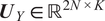
$ {\boldsymbol{U}}_Y\in {\mathrm{\mathbb{R}}}^{2N\times K} $
in the main diagonal,
$ {\boldsymbol{U}}_Y\in {\mathrm{\mathbb{R}}}^{2N\times K} $
 contains the left singular vectors,
$ {\varSigma}_Y\in {\mathrm{\mathbb{R}}}^{K\times K} $
contains the left singular vectors,
$ {\varSigma}_Y\in {\mathrm{\mathbb{R}}}^{K\times K} $
 is a diagonal matrix that stores the singular values, and
$ {\boldsymbol{V}}_Y\in {\mathrm{\mathbb{R}}}^{K\times K} $
is a diagonal matrix that stores the singular values, and
$ {\boldsymbol{V}}_Y\in {\mathrm{\mathbb{R}}}^{K\times K} $
 contains the right singular vectors. The scaled POD eigenmodes
$ {U}_{Y,k}\left(\boldsymbol{x}\right) $
contains the right singular vectors. The scaled POD eigenmodes
$ {U}_{Y,k}\left(\boldsymbol{x}\right) $
 are extracted from the columns of
$ {\boldsymbol{U}}_Y $
are extracted from the columns of
$ {\boldsymbol{U}}_Y $
 :
:

and the time coefficients are extracted from
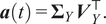
The fluctuating velocity field can be written as

where
$ {m}_u\left(\ll K\right) $
 is the number of retained POD modes,
$ {a}_k(t) $
is the number of retained POD modes,
$ {a}_k(t) $
 is the time coefficient of the
$ k $
is the time coefficient of the
$ k $
 -th POD mode, and
$ {U}_{Y,k}^{(i)} $
-th POD mode, and
$ {U}_{Y,k}^{(i)} $
 is the
$ k $
is the
$ k $
 -th POD eigenmode of the
$ i $
-th POD eigenmode of the
$ i $
 -th velocity component. This expression can be written in the matrix form as

or more compactly

2.2. Computation of the time-delayed Hankel coefficients
Using the POD coefficients from the training dataset, we assemble the time-delayed Hankel matrix
$ \boldsymbol{H} $
 :
:

where we use
$ q $
 vectors of
$ {m}_u $
vectors of
$ {m}_u $
 POD coefficients in each column. The number of columns is
$ p={K}_{\mathrm{train}}-q+1 $
POD coefficients in each column. The number of columns is
$ p={K}_{\mathrm{train}}-q+1 $
 , where
$ {K}_{\mathrm{train}} $
, where
$ {K}_{\mathrm{train}} $
 is the number of snapshots for the training dataset; thus,
$ \boldsymbol{H}\in {\mathrm{\mathbb{R}}}^{\left({m}_u\times q\right)\times p} $
is the number of snapshots for the training dataset; thus,
$ \boldsymbol{H}\in {\mathrm{\mathbb{R}}}^{\left({m}_u\times q\right)\times p} $
 . Performing SVD on
$ \boldsymbol{H} $
. Performing SVD on
$ \boldsymbol{H} $
 we obtain,

where
$ {\boldsymbol{U}}_H\in {\mathrm{\mathbb{R}}}^{\left({m}_u\times q\right)\times r} $
 ,
$ {\boldsymbol{\Sigma}}_H\in {\mathrm{\mathbb{R}}}^{r\times r} $
,
$ {\boldsymbol{\Sigma}}_H\in {\mathrm{\mathbb{R}}}^{r\times r} $
 ,
$ {\boldsymbol{V}}_H\in {\mathrm{\mathbb{R}}}^{p\times r} $
,
$ {\boldsymbol{V}}_H\in {\mathrm{\mathbb{R}}}^{p\times r} $
 and
$ r $
and
$ r $
 is the number of retained singular values. The matrix
$ {\boldsymbol{U}}_H $
is the number of retained singular values. The matrix
$ {\boldsymbol{U}}_H $
 of the left singular vectors can be explicitly written as

where each column
$ {\boldsymbol{U}}_{H,i}^{\left(u,v\right)}\left({t}_1:{t}_q\right)\in {\mathrm{\mathbb{R}}}^{m_u} $
 is the
$ i $
is the
$ i $
 -th delayed singular mode. The matrix of the right singular vectors
$ {\boldsymbol{V}}_H $
-th delayed singular mode. The matrix of the right singular vectors
$ {\boldsymbol{V}}_H $
 can be explicitly written as

2.3. Construction of a dynamical system for POD coefficients
The next step is the construction of a linear dynamical system that describes the evolution of the POD coefficients. We first describe two algorithms, linear 1 and linear 2, that extract linear models for the right singular vectors in matrix
$ {\boldsymbol{V}}_H $
 . A schematic of the two algorithms is presented in Figure 1. We then briefly describe an algorithm based on the n4sid system identification method.
Schematic overview of the algorithms linear 1 and linear 2.

Figure 1. Long description
The diagram is organized into several stages of data processing.
1. Top Section: Flow field data is shown as a stack of three heatmaps labeled k equals 1, k equals 2, and k equals K, representing Y(x, t sub k). An arrow points to an Economy S V D section where V super 1/2 Y is approximately equal to U sub Y, Sigma sub Y, and V sub Y super T. Dimensions are labeled as 2 N, K, and m sub u.
2. Middle Left Section: True output a[k] is shown as four oscillating waveforms for m equals 1 through 4. Below this, four heatmaps show u prime and v prime components for U sub Y,1 and U sub Y,2. At the bottom left, sensor measurements for u prime and v prime are plotted as red and blue waves, labeled as sensor input s[k].
3. Middle Right Section: The Economy S V D output feeds into Delayed coordinates, forming a matrix H. This matrix undergoes another Economy S V D to produce U sub H, Sigma sub H, and V sub H super T with rank r.
4. Branching Logic: The process splits into two paths based on rank r sub H.
* Path 1 (if r sub H equals r minus 1): Shows a partitioned matrix A sub 1 and B sub 1, leading to the Linear 1 model equations involving v sub H,1:r-1[k + 1] and a[k].
* Path 2 (else if r sub H equals r): Shows a single matrix A sub 2, leading to the Linear 2 model equations involving v sub H[k + 1] and a[k].
5. Bottom Section: Both paths converge to define parameters (A, C) and Q. These parameters, along with measurement noise g[k] and sensor input s[k], feed into a final box labeled Kalman filter. The filter contains equations for the state estimate v-hat, the output estimate a-hat, and the sensor estimate s-hat using the S U sub Y transformation.
2.3.1. First linear model based on time-delayed Hankel coefficients (linear 1)
We now define the vector
$ {\boldsymbol{v}}_{H,1:r-1}\left({t}_j\right)={\left[{v}_{H,1}\left({t}_j\right),{v}_{H,2}\left({t}_j\right),\dots, {v}_{H,r-1}\left({t}_j\right)\right]}^{\top}\in {\mathrm{\mathbb{R}}}^{r-1} $ $ \left(j=1\dots p\right) $
 extracted from the columns of matrix
$ {\boldsymbol{V}}_H $
extracted from the columns of matrix
$ {\boldsymbol{V}}_H $
 . We consider
$ {\boldsymbol{v}}_{H,1:r-1} $
. We consider
$ {\boldsymbol{v}}_{H,1:r-1} $
 as the state variable and formulate the discrete in time, forced, linear dynamical system,

where
$ {\boldsymbol{v}}_{H,1:r-1}\left[k\right]={\boldsymbol{v}}_{H,1:r-1}\left[{t}_k\right] $
 ,
$ k=1\dots p-1 $
,
$ k=1\dots p-1 $
 . We build a linear model using only the first (
$ r-1 $
. We build a linear model using only the first (
$ r-1 $
 ) elements of each column of
$ {\boldsymbol{V}}_H $
) elements of each column of
$ {\boldsymbol{V}}_H $
 , while the last element is used as forcing term.
The system matrices
$ {\boldsymbol{A}}_1\in {\mathrm{\mathbb{R}}}^{\left(r-1\right)\times \left(r-1\right)} $
 and
$ {\boldsymbol{B}}_1\in {\mathrm{\mathbb{R}}}^{\left(r-1\right)} $
and
$ {\boldsymbol{B}}_1\in {\mathrm{\mathbb{R}}}^{\left(r-1\right)} $
 are computed by writing Eq. (2.12) explicitly for
$ k=1 $
are computed by writing Eq. (2.12) explicitly for
$ k=1 $
 to
$ p-1 $
to
$ p-1 $
 ,
,


The above set can be written in matrix form as

where
$ {\boldsymbol{V}}_{1:r-1}^{\prime },{\boldsymbol{V}}_{1:r-1}\in {\mathrm{\mathbb{R}}}^{\left(r-1\right)\times \left(p-1\right)} $
 and
$ {\boldsymbol{V}}_r\in {\mathrm{\mathbb{R}}}^{p-1} $
and
$ {\boldsymbol{V}}_r\in {\mathrm{\mathbb{R}}}^{p-1} $
 take the following forms:


Eq. (2.14) can be written in a more compact form as

where
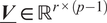
$ \boldsymbol{D}\in {\mathrm{\mathbb{R}}}^{\left(r-1\right)\times r} $
 and
$ \underline {\boldsymbol{V}}\in {\mathrm{\mathbb{R}}}^{r\times \left(p-1\right)} $
and
$ \underline {\boldsymbol{V}}\in {\mathrm{\mathbb{R}}}^{r\times \left(p-1\right)} $
 . In matrix
$ \boldsymbol{D} $
. In matrix
$ \boldsymbol{D} $
 , the first (
$ r-1 $
, the first (
$ r-1 $
 ) columns represent
$ {\boldsymbol{A}}_1 $
) columns represent
$ {\boldsymbol{A}}_1 $
 and the last column represents
$ {\boldsymbol{B}}_1 $
and the last column represents
$ {\boldsymbol{B}}_1 $
 . So we have

Once
$ {\boldsymbol{B}}_1 $
 is known, the forcing
$ {\boldsymbol{B}}_1{\boldsymbol{v}}_{H,r}\left[k\right] $
is known, the forcing
$ {\boldsymbol{B}}_1{\boldsymbol{v}}_{H,r}\left[k\right] $
 can be easily computed from the training dataset. The covariance matrix of the forcing
$ {\boldsymbol{Q}}_1\in {\mathrm{\mathbb{R}}}^{\left(r-1\right)\times \left(r-1\right)} $
can be easily computed from the training dataset. The covariance matrix of the forcing
$ {\boldsymbol{Q}}_1\in {\mathrm{\mathbb{R}}}^{\left(r-1\right)\times \left(r-1\right)} $
 can be obtained from

Vector
$ {\boldsymbol{v}}_{H,1:r-1}\left[k\right] $
 can be used to obtain the POD coefficients at the
$ k $
can be used to obtain the POD coefficients at the
$ k $
 -th instant from

where
$ {\boldsymbol{C}}_1\in {\mathrm{\mathbb{R}}}^{m_u\times \left(r-1\right)} $
 and matrix
$ {\boldsymbol{U}}_{H,1:r-1}\left({t}_1\right) $
and matrix
$ {\boldsymbol{U}}_{H,1:r-1}\left({t}_1\right) $
 consists of the
$ \left(r-1\right) $
consists of the
$ \left(r-1\right) $
 elements of the top row of
$ {\boldsymbol{U}}_H $
elements of the top row of
$ {\boldsymbol{U}}_H $
 , i.e.,

2.3.2. Second linear model based on time-delayed Hankel coefficients (linear 2)
In the second linear model, the state variable is
$ {\boldsymbol{v}}_H\left({t}_j\right)={\left[{v}_{H,1}\left({t}_j\right),{v}_{H,2}\left({t}_j\right),\dots, {v}_{H,r}\left({t}_j\right)\right]}^{\top}\in {\mathrm{\mathbb{R}}}^r $ $ \left(j=1\dots p\right) $
 , i.e., we consider all
$ r $
, i.e., we consider all
$ r $
 elements of each column of matrix
$ {\boldsymbol{V}}_H $
elements of each column of matrix
$ {\boldsymbol{V}}_H $
 . This model was first presented in Lu and Papadakis (Reference Lu and Papadakis2026a), but it is repeated below for completeness. A schematic overview of the algorithm is presented in Figure 1.
We seek a linear model of the form

where
$ {\boldsymbol{w}}_2\left[k\right] $
 is random forcing. To obtain
$ {\boldsymbol{A}}_2\in {\mathrm{\mathbb{R}}}^{r\times r} $
is random forcing. To obtain
$ {\boldsymbol{A}}_2\in {\mathrm{\mathbb{R}}}^{r\times r} $
 , we write Eq. (2.21) explicitly for
$ k=1 $
, we write Eq. (2.21) explicitly for
$ k=1 $
 to
$ p-1 $
to
$ p-1 $
 :
:


In matrix form, this becomes

where
$ {\boldsymbol{V}}^{\prime },\boldsymbol{V}\in {\mathrm{\mathbb{R}}}^{r\times \left(p-1\right)} $
 .
.


Then, system matrix
$ {\boldsymbol{A}}_2 $
 can be calculated by

Once
$ {\boldsymbol{A}}_2 $
 is known, the forcing
$ {\boldsymbol{w}}_2\left[k\right] $
is known, the forcing
$ {\boldsymbol{w}}_2\left[k\right] $
 can be easily calculated from the training dataset,
$ {\boldsymbol{w}}_2\left[k\right]={\boldsymbol{v}}_H\left[k+1\right]-{\boldsymbol{A}}_2{\boldsymbol{v}}_H\left[k\right] $
can be easily calculated from the training dataset,
$ {\boldsymbol{w}}_2\left[k\right]={\boldsymbol{v}}_H\left[k+1\right]-{\boldsymbol{A}}_2{\boldsymbol{v}}_H\left[k\right] $
 . As before, the covariance matrix
$ {\boldsymbol{Q}}_2\in {\mathrm{\mathbb{R}}}^{r\times r} $
. As before, the covariance matrix
$ {\boldsymbol{Q}}_2\in {\mathrm{\mathbb{R}}}^{r\times r} $
 of
$ {\boldsymbol{w}}_2 $
of
$ {\boldsymbol{w}}_2 $
 can be obtained from,

From vector
$ {\boldsymbol{v}}_H\left[k\right] $
 , we can get

where
$ {\boldsymbol{C}}_2\in {\mathrm{\mathbb{R}}}^{m_u\times r} $
 and
$ {\boldsymbol{U}}_H\left({t}_1\right) $
and
$ {\boldsymbol{U}}_H\left({t}_1\right) $
 is the top row of
$ {\boldsymbol{U}}_H $
is the top row of
$ {\boldsymbol{U}}_H $
 .
.
2.3.3. N4sid algorithm
A schematic overview of this algorithm is displayed in Figure 2. In n4sid, we seek a linear dynamical system of the form

where
$ \boldsymbol{a}\left[k\right]=\boldsymbol{a}\left({t}_K\right) $
 ,
$ \boldsymbol{x}\in {\mathrm{\mathbb{R}}}^n $
,
$ \boldsymbol{x}\in {\mathrm{\mathbb{R}}}^n $
 is the internal state vector of size
$ n $
is the internal state vector of size
$ n $
 ,
$ \boldsymbol{A}\in {\mathrm{\mathbb{R}}}^{n\times n} $
,
$ \boldsymbol{A}\in {\mathrm{\mathbb{R}}}^{n\times n} $
 and
$ \boldsymbol{C}\in {\mathrm{\mathbb{R}}}^{m_u\times n} $
and
$ \boldsymbol{C}\in {\mathrm{\mathbb{R}}}^{m_u\times n} $
 ,
$ \boldsymbol{w}\left[k\right]\in {\mathrm{\mathbb{R}}}^n $
,
$ \boldsymbol{w}\left[k\right]\in {\mathrm{\mathbb{R}}}^n $
 and
$ \boldsymbol{v}\left[k\right]\in {\mathrm{\mathbb{R}}}^{m_u} $
and
$ \boldsymbol{v}\left[k\right]\in {\mathrm{\mathbb{R}}}^{m_u} $
 are Gaussian white noise sequences. Note that we have introduced the internal state
$ \boldsymbol{x}\left[k\right] $
are Gaussian white noise sequences. Note that we have introduced the internal state
$ \boldsymbol{x}\left[k\right] $
 with size
$ n $
with size
$ n $
 , which is independent of the total number of retained POD modes,
$ {m}_u $
, which is independent of the total number of retained POD modes,
$ {m}_u $
 . This gives additional flexibility, as it allows one to adjust
$ n $
. This gives additional flexibility, as it allows one to adjust
$ n $
 and thus the size of the matrices
$ \boldsymbol{A} $
and thus the size of the matrices
$ \boldsymbol{A} $
 and
$ \boldsymbol{C} $
and
$ \boldsymbol{C} $
 , so that (2.28) returns a vector sequence
$ \boldsymbol{a}\left[k\right] $
, so that (2.28) returns a vector sequence
$ \boldsymbol{a}\left[k\right] $
 that optimally fits the true values.
Schematic overview of the algorithm based on the system identification method n4sid.

Figure 2. Long description
The flowchart is organized into three main horizontal stages.
Top row: Flow field data is shown as a stack of three heatmaps labeled k equals 1, k equals 2, and k equals K. An arrow points to an Economy S V D section where a large blue matrix V super 1/2 Y is approximately decomposed into three smaller matrices: U sub Y, Sigma sub Y (a diagonal matrix in a red dashed box), and V sub Y super T.
Middle row: An arrow from V sub Y super T leads to a set of four time-series plots labeled True output: a[k] for m equals 1 through 4. These plots feed into an n 4 s i d block, which outputs a Plant state-space model: x[k plus 1] equals A x[k] plus w[k] and a[k] equals C x[k] plus v[k]. Below the true output, four heatmaps labeled U sub Y, 1 and U sub Y, 2 for variables u prime and v prime are multiplied by the true output to produce S U sub Y.
Bottom row: Sensor measurements are shown as two line graphs with red and blue waves. These provide the sensor input s[k]. The plant model parameters (A, C) and Q, along with measurement noise g[k] and R, feed into a Kalman filter block. The filter contains the equations: x-hat[k plus 1] equals A x-hat[k] plus L (s[k] minus s-hat[k]) and a-hat[k] equals C x-hat[k].
We use the system identification algorithm n4sid to obtain
$ \boldsymbol{A} $
 and
$ \boldsymbol{C} $
and
$ \boldsymbol{C} $
 , as well as the covariance matrices of sequences
$ \boldsymbol{w}\left[k\right] $
, as well as the covariance matrices of sequences
$ \boldsymbol{w}\left[k\right] $
 and
$ \boldsymbol{v}\left[k\right] $
and
$ \boldsymbol{v}\left[k\right] $
 . The algorithm also assembles the time-delayed Hankel matrix (2.8) and considers the top
$ q/2 $
. The algorithm also assembles the time-delayed Hankel matrix (2.8) and considers the top
$ q/2 $
 rows as past outputs and the bottom
$ q/2 $
rows as past outputs and the bottom
$ q/2 $
 as future outputs. The next step is the orthogonal projection of the row space of the future outputs into the row space of the past outputs and the SVD of the resulting matrix. In many cases, there is only a small number of large singular values and the rest can be discarded; this yields an optimal order
$ n $
as future outputs. The next step is the orthogonal projection of the row space of the future outputs into the row space of the past outputs and the SVD of the resulting matrix. In many cases, there is only a small number of large singular values and the rest can be discarded; this yields an optimal order
$ n $
 . Alternatively, the order
$ n $
. Alternatively, the order
$ n $
 can be prescribed. From the left and right singular vectors, the states
$ \boldsymbol{x}\left[k\right] $
can be prescribed. From the left and right singular vectors, the states
$ \boldsymbol{x}\left[k\right] $
 are obtained, and then, the matrices
$ \boldsymbol{A},\boldsymbol{C} $
are obtained, and then, the matrices
$ \boldsymbol{A},\boldsymbol{C} $
 are computed using least squares. Note that
$ \boldsymbol{A} $
are computed using least squares. Note that
$ \boldsymbol{A} $
 and
$ \boldsymbol{C} $
and
$ \boldsymbol{C} $
 are unique up to a similarity transformation. More details can be found in Van Overschee and De Moor (Reference Van Overschee and De Moor1994) and the book of Van Overschee and De Moor (Reference Van Overschee and De Moor1996), in particular chapter 3 that deals with stochastic identification (i.e., when only output data are available, as in our case). The algorithm is implemented in MATLAB and can be executed with the command n4sid.
In conclusion, n4sid also starts with the same Hankel matrix (2.8) as the previous two algorithms, but then follows a different path. The states
$ \boldsymbol{x}\left[k\right] $
 are obtained directly from the output vectors, and then the system matrices are computed. On the other hand, for linear 1 and linear 2, the dominant modes of (2.8) are first determined, and then, a system is constructed from the evolution of the modal coefficients.
2.4. Closure of the systems using sensor measurements
The linear systems (2.12), (2.21), or (2.28) cannot be used directly because the forcing terms are unknown. However, if sensor measurements are available, they can be used to close the systems. This is achieved as explained below.
Let us assume that we have a set of
$ l $
 velocity measurements
$ \boldsymbol{s}\left[k\right]\in {\mathrm{\mathbb{R}}}^l $
velocity measurements
$ \boldsymbol{s}\left[k\right]\in {\mathrm{\mathbb{R}}}^l $
 at a number of sensor points. At each sensor, one or more velocity components are recorded. We can express
$ \boldsymbol{s}\left[k\right] $
at a number of sensor points. At each sensor, one or more velocity components are recorded. We can express
$ \boldsymbol{s}\left[k\right] $
 in terms of
$ \boldsymbol{a}\left[k\right] $
in terms of
$ \boldsymbol{a}\left[k\right] $
 as follows

where matrix
$ \boldsymbol{S} $
 selects the rows of the POD mode matrix
$ {\boldsymbol{U}}_Y $
selects the rows of the POD mode matrix
$ {\boldsymbol{U}}_Y $
 (see (2.7)) corresponding to the sensor location and the velocity component being measured (it is
$ 0 $
(see (2.7)) corresponding to the sensor location and the velocity component being measured (it is
$ 0 $
 everywhere except for those points and components where the corresponding element is equal to
$ 1 $
everywhere except for those points and components where the corresponding element is equal to
$ 1 $
 ). Vector
$ \boldsymbol{g}\in {\mathrm{\mathbb{R}}}^l $
). Vector
$ \boldsymbol{g}\in {\mathrm{\mathbb{R}}}^l $
 includes measurement errors as well as errors due to POD mode truncation (because only
$ {m}_u $
includes measurement errors as well as errors due to POD mode truncation (because only
$ {m}_u $
 modes are retained). Here, we assume that
$ \boldsymbol{g}\left[k\right] $
modes are retained). Here, we assume that
$ \boldsymbol{g}\left[k\right] $
 arises only due to the POD truncation; thus, the elements of
$ \boldsymbol{g}\left[k\right] $
arises only due to the POD truncation; thus, the elements of
$ \boldsymbol{g}\left[k\right] $
 can be obtained from the training dataset,
$ \boldsymbol{g}\left[k\right]=\boldsymbol{s}\left[k\right]-{\boldsymbol{SU}}_Y\boldsymbol{a}\left[k\right] $
can be obtained from the training dataset,
$ \boldsymbol{g}\left[k\right]=\boldsymbol{s}\left[k\right]-{\boldsymbol{SU}}_Y\boldsymbol{a}\left[k\right] $
 . However, this is not a restriction; sensor noise can be easily included. The covariance
$ \boldsymbol{R}\in {\mathrm{\mathbb{R}}}^{l\times l} $
. However, this is not a restriction; sensor noise can be easily included. The covariance
$ \boldsymbol{R}\in {\mathrm{\mathbb{R}}}^{l\times l} $
 can be easily calculated from

We are now ready to design a Kalman filter to estimate
$ {\boldsymbol{v}}_{H,1:{r}_H}\left[k\right] $
 from the sparse measurements
$ \boldsymbol{s}\left[k\right] $
from the sparse measurements
$ \boldsymbol{s}\left[k\right] $
 , where
$ {r}_H $
, where
$ {r}_H $
 is either
$ \left(r-1\right) $
is either
$ \left(r-1\right) $
 or
$ r $
or
$ r $
 depending on whether the forcing uses the
$ r $
depending on whether the forcing uses the
$ r $
 -th element (linear 1) or it is random (linear 2), respectively. In either case, the filter takes the form


The hat
$ \hat{\left(\cdot \right)} $
 denotes an estimated quantity and
$ \mathrm{\mathcal{L}}\in $
denotes an estimated quantity and
$ \mathrm{\mathcal{L}}\in $ $ {\mathrm{\mathbb{R}}}^{r_H\times l} $
 is the Kalman filter gain. The latter is obtained from the solution of the following Riccati equation:


We use the same idea to close the n4sid system (2.28).
3. Assimilation of sparse scalar measurements
We now proceed to describe the algorithm for assimilating scalar measurements. We start by obtaining the scalar POD modes following the same approach as for the velocity modes. The snapshot matrix
$ \boldsymbol{Z}\left(\boldsymbol{x},{t}_1:{t}_K\right) $
 for the scalar fluctuations
$ {c}^{\prime } $
for the scalar fluctuations
$ {c}^{\prime } $
 is
is

where
$ \boldsymbol{Z}\in {\mathrm{\mathbb{R}}}^{N\times K} $
 . The scalar field data are synchronized with the velocity data, i.e., the time instants
$ {t}_i\;\left(i=1\dots K\right) $
. The scalar field data are synchronized with the velocity data, i.e., the time instants
$ {t}_i\;\left(i=1\dots K\right) $
 in (2.1) and (3.1) are the same. As before, we apply SVD to the weighted matrix
$ {\mathcal{V}}^{1/2}\boldsymbol{Z} $
in (2.1) and (3.1) are the same. As before, we apply SVD to the weighted matrix
$ {\mathcal{V}}^{1/2}\boldsymbol{Z} $
 (where now
$ \mathcal{V}=\operatorname{diag}\left({V}_1,{V}_2\dots {V}_N\right) $
(where now
$ \mathcal{V}=\operatorname{diag}\left({V}_1,{V}_2\dots {V}_N\right) $
 ) and obtain the scalar POD modes,
$ {U}_{Z,k}\left(x,y\right) $
) and obtain the scalar POD modes,
$ {U}_{Z,k}\left(x,y\right) $
 , and time coefficients,
$ {b}_k(t) $
, and time coefficients,
$ {b}_k(t) $
 . Thus we can write

where
$ {m}_c $
 is the number of retained scalar POD modes, or in more compact form,

Equations (2.7) and (3.3) can be written together as

We then build the time-delayed Hankel matrix with the POD coefficients of the most dominant
$ {m}_u $
 velocity and
$ {m}_c $
velocity and
$ {m}_c $
 scalar modes:

where
$ \boldsymbol{H}\in {\mathrm{\mathbb{R}}}^{\left({m}_u+{m}_c\right)q\times p} $
 . Performing SVD on
$ \boldsymbol{H} $
. Performing SVD on
$ \boldsymbol{H} $
 , we obtain the matrices
$ {\boldsymbol{U}}_H $
, we obtain the matrices
$ {\boldsymbol{U}}_H $
 ,
$ {\boldsymbol{\Sigma}}_H $
,
$ {\boldsymbol{\Sigma}}_H $
 ,
$ {\boldsymbol{V}}_H $
,
$ {\boldsymbol{V}}_H $
 ,
,

as before. The matrix of the left singular vectors
$ {\boldsymbol{U}}_H\in {\mathrm{\mathbb{R}}}^{\left(\left({m}_u+{m}_c\right)\times q\right)\times r} $
 can be written explicitly as

Two dynamical systems for
$ {\boldsymbol{v}}_H $
 can be derived as before. Also, the process noise covariance
$ \boldsymbol{Q}\in {\mathrm{\mathbb{R}}}^{r\times r} $
can be derived as before. Also, the process noise covariance
$ \boldsymbol{Q}\in {\mathrm{\mathbb{R}}}^{r\times r} $
 can be calculated in the same way as in section 2. Vector
$ {\boldsymbol{v}}_H\left[k\right] $
can be calculated in the same way as in section 2. Vector
$ {\boldsymbol{v}}_H\left[k\right] $
 can be used to obtain the POD coefficients of the velocity and scalar fields at the
$ k $
can be used to obtain the POD coefficients of the velocity and scalar fields at the
$ k $
 -th instant as

where
$ \boldsymbol{C}\in {\mathrm{\mathbb{R}}}^{\left({m}_u+{m}_c\right)\times r} $
 and matrix
$ {\boldsymbol{U}}_H\left({t}_1\right) $
and matrix
$ {\boldsymbol{U}}_H\left({t}_1\right) $
 represents the top two rows of
$ {\boldsymbol{U}}_H $
represents the top two rows of
$ {\boldsymbol{U}}_H $
 , i.e.,

Let us assume that we have now
$ l $
 scalar measurements
$ \boldsymbol{s}\left[k\right] $
scalar measurements
$ \boldsymbol{s}\left[k\right] $
 ; they can be written as

where now matrix
$ \boldsymbol{S} $
 selects the rows of the POD mode matrix
$ {\boldsymbol{U}}_Z $
selects the rows of the POD mode matrix
$ {\boldsymbol{U}}_Z $
 corresponding to the scalar sensor locations. Note that it is possible to mix velocity and scalar measurements; in this case,
$ \boldsymbol{S} $
corresponding to the scalar sensor locations. Note that it is possible to mix velocity and scalar measurements; in this case,
$ \boldsymbol{S} $
 will act on the compound matrix
$ {\boldsymbol{U}}_{YZ} $
will act on the compound matrix
$ {\boldsymbol{U}}_{YZ} $
 (see (3.4)). In the following, we assume that we have scalar measurements only. The covariance
$ \boldsymbol{R} $
(see (3.4)). In the following, we assume that we have scalar measurements only. The covariance
$ \boldsymbol{R} $
 of vector
$ \boldsymbol{g} $
of vector
$ \boldsymbol{g} $
 can be obtained as explained in the previous section.
The Kalman filter takes the form


where
$ {\left(\boldsymbol{C}\right)}_2 $
 indicates the second row block of matrix
$ \boldsymbol{C} $
indicates the second row block of matrix
$ \boldsymbol{C} $
 and the Kalman gain matrix
$ \mathrm{\mathcal{L}} $
and the Kalman gain matrix
$ \mathrm{\mathcal{L}} $
 is obtained by solving a Riccati equation similar to (2.32) where
$ {\boldsymbol{U}}_Y $
is obtained by solving a Riccati equation similar to (2.32) where
$ {\boldsymbol{U}}_Y $
 is replaced by
$ {\boldsymbol{U}}_Z $
is replaced by
$ {\boldsymbol{U}}_Z $
 .
.
We similarly augment the output of the n4sid system (2.28) with the scalar POD modes, identify all matrices, and apply Kalman filter to close the system. All the details can be found in Lu and Papadakis, Reference Lu and Papadakis2023.
4. Forecasting of POD coefficients from current measurements
In the previous two sections we demonstrated how to obtain coefficients
$ \boldsymbol{a}\left[k\right] $
 and
$ \boldsymbol{b}\left[k\right] $
and
$ \boldsymbol{b}\left[k\right] $
 from
$ {\boldsymbol{v}}_H\left[k\right] $
from
$ {\boldsymbol{v}}_H\left[k\right] $
 ; see equations (2.19), (2.27), and (3.8). This was achieved by considering only the top row (or the top block of two rows) of matrix
$ {\boldsymbol{U}}_H $
; see equations (2.19), (2.27), and (3.8). This was achieved by considering only the top row (or the top block of two rows) of matrix
$ {\boldsymbol{U}}_H $
 of linear 1 and linear 2 models. By considering the rest of the rows, one can also obtain the POD coefficients at
$ q-1 $
of linear 1 and linear 2 models. By considering the rest of the rows, one can also obtain the POD coefficients at
$ q-1 $
 later time instants, i.e., one can forecast the future evolution of the coefficients from current sensor data. Indeed, using (3.6) and the estimated
$ {\hat{\boldsymbol{v}}}_{H,1:{r}_H}\left[k\right] $
later time instants, i.e., one can forecast the future evolution of the coefficients from current sensor data. Indeed, using (3.6) and the estimated
$ {\hat{\boldsymbol{v}}}_{H,1:{r}_H}\left[k\right] $
 , we get

We now proceed to assess the performance of the estimation strategies based on linear 1, linear 2, and n4sid models. We also examine the quality of flow forecasting from sparse scalar measurements.
5. Computational setup, numerical methodology, and basic flow features
We consider the 2D flow around a surface-mounted prism with height
$ h $
 . The computational domain has dimensions
$ 19h\times 10h $
. The computational domain has dimensions
$ 19h\times 10h $
 . The origin of the coordinate system is located at the bottom-left corner of the prism. The inlet is located at
$ x/h=-6 $
. The origin of the coordinate system is located at the bottom-left corner of the prism. The inlet is located at
$ x/h=-6 $
 and the outlet at
$ x/h=13 $
and the outlet at
$ x/h=13 $
 . The domain extends up to
$ y/h=10 $
. The domain extends up to
$ y/h=10 $
 in the wall-normal direction. Uniform velocity
$ {U}_{\infty }=1 $
in the wall-normal direction. Uniform velocity
$ {U}_{\infty }=1 $
 is prescribed at the inlet and a convective boundary condition at the outlet. No-slip conditions are imposed on the prism surfaces and bottom wall, while symmetry conditions are applied on the top boundary. Scalar is released from a circular source centered at
$ \left({x}_s,{y}_s\right)=\left(-\mathrm{2,0.2}\right)h $
is prescribed at the inlet and a convective boundary condition at the outlet. No-slip conditions are imposed on the prism surfaces and bottom wall, while symmetry conditions are applied on the top boundary. Scalar is released from a circular source centered at
$ \left({x}_s,{y}_s\right)=\left(-\mathrm{2,0.2}\right)h $
 , with radius
$ 0.1h $
, with radius
$ 0.1h $
 . The source strength (amount of scalar released per unit volume) is equal to 10. The Reynolds number, defined as
$ {\mathit{\operatorname{Re}}}_h={U}_{\infty }h/\nu $
. The source strength (amount of scalar released per unit volume) is equal to 10. The Reynolds number, defined as
$ {\mathit{\operatorname{Re}}}_h={U}_{\infty }h/\nu $
 , is set to
$ 1000 $
, is set to
$ 1000 $
 .
.
The flow is simulated with the in-house code PANTARHEI. The incompressible Navier–Stokes equations are discretized in space using the finite volume method, with a second-order central discretization scheme (for both convection and viscous terms), and marched in time with a third-order backward scheme. The fractional step method is employed to obtain pressure and correct the velocities to satisfy the continuity equation. The code has been used extensively to simulate transitional and turbulent flows (Thomareis and Papadakis, Reference Thomareis and Papadakis2017, Reference Thomareis and Papadakis2018; Yao and Papadakis, Reference Yao and Papadakis2023; Schlander et al., Reference Schlander, Rigopoulos and Papadakis2024).
The flow domain is discretized using
$ {N}_x\times {N}_y=576\times 268 $
 Cartesian cells, which are clustered close to the prism surfaces and the bottom wall. The time step
$ \Delta t=0.005 $
Cartesian cells, which are clustered close to the prism surfaces and the bottom wall. The time step
$ \Delta t=0.005 $
 is selected to satisfy
$ \mathrm{CFL}<0.5 $
is selected to satisfy
$ \mathrm{CFL}<0.5 $
 . The cell thickness is
$ 0.006h $
. The cell thickness is
$ 0.006h $
 in the first layer near the wall. This resolution provides grid-independent results, Lu and Papadakis (Reference Lu and Papadakis2023). The flow is first advanced for three flow-through times (one flow-through time is
$ 19 $
in the first layer near the wall. This resolution provides grid-independent results, Lu and Papadakis (Reference Lu and Papadakis2023). The flow is first advanced for three flow-through times (one flow-through time is
$ 19 $
 time units
$ h/{U}_{\infty } $
time units
$ h/{U}_{\infty } $
 ), and the simulation is then restarted and advanced for 190 more time units (10 more flow-through times).
Snapshots of velocities and scalar fields are collected within a subregion
$ \left[-3h,10h\right]\times \left[0,4h\right] $
 that contains
$ N=\mathrm{72,674} $
that contains
$ N=\mathrm{72,674} $
 cells for further processing. In total,
$ 4750 $
cells for further processing. In total,
$ 4750 $
 flow and scalar field snapshots are recorded synchronously during the last 10 flow-through times. The time separation between successive snapshots is
$ 0.04\frac{h}{U_{\infty }} $
flow and scalar field snapshots are recorded synchronously during the last 10 flow-through times. The time separation between successive snapshots is
$ 0.04\frac{h}{U_{\infty }} $
 . The snapshots are split into two even datasets, one for training and the other for validation purposes, i.e.,
$ {K}_{\mathrm{train}}=2375 $
. The snapshots are split into two even datasets, one for training and the other for validation purposes, i.e.,
$ {K}_{\mathrm{train}}=2375 $
 .
.
The wake consists of periodically shed concentrated vortices that are separated by stretched shear layers, as shown in contours of instantaneous vorticity in Figure 3(a). These vortices also disperse the scalar, as shown in Figure 3(b). The dominant frequencies are
$ St=0.063 $
 and its harmonics
$ 0.126 $
and its harmonics
$ 0.126 $
 ,
$ 0.189 $
,
$ 0.189 $
 , and so forth. Sensors are placed at the peaks of the velocity POD modes. Modes 1 and 2 have large footprint close to the cube, while modes 3–5 are dominant further downstream; for details, see Lu and Papadakis (Reference Lu and Papadakis2023). At the sensor locations, either both
$ {u}^{\prime }(t) $
, and so forth. Sensors are placed at the peaks of the velocity POD modes. Modes 1 and 2 have large footprint close to the cube, while modes 3–5 are dominant further downstream; for details, see Lu and Papadakis (Reference Lu and Papadakis2023). At the sensor locations, either both
$ {u}^{\prime }(t) $
 and
$ {v}^{\prime }(t) $
and
$ {v}^{\prime }(t) $
 or only
$ {c}^{\prime }(t) $
or only
$ {c}^{\prime }(t) $
 is recorded. The locations of the first five sensors are shown in Figure 3.
Instantaneous (a) vorticity and (b) scalar fields at the same time instant. Square markers (■) indicate sensor locations.

Figure 3. Long description
The two panels share a horizontal x forward slash h axis from negative 2 to 10 and a vertical y forward slash h axis from 0 to 4. A gray square obstacle is positioned at the base between x forward slash h equals 0 and 1.
Panel a shows the vorticity field. A color bar on the right ranges from negative 6 in dark blue to 6 in dark red. A large blue clockwise vortex is centered near x forward slash h equals 6 and y forward slash h equals 2.5, preceded by a thin red shear layer. Smaller turbulent structures are visible immediately behind the obstacle.
Panel b shows the scalar field. A color bar on the right ranges from 0 in dark blue to 8 in dark red. The field shows a plume of higher scalar values originating from the obstacle and diffusing into the wake, following the same general shape as the vorticity structures but with less defined internal gradients.
Both panels feature five black square sensors labeled 1 through 5. Sensors 1 and 2 are stacked vertically at x forward slash h equals 2.5. Sensor 3 is at x forward slash h equals 8.5 and y forward slash h equals 2.5. Sensors 4 and 5 are stacked vertically at x forward slash h equals 9.5.
6. Results and discussion
6.1. Assessment of reconstruction quality of different linear models
We now compare the reconstruction quality of the three estimators based on models linear 1, linear 2, and n4sid. The former two have different forcing terms, as explained in Section 2. Due to this difference, linear 1 has order (
$ r-1 $
 ) and linear 2 has order
$ r $
) and linear 2 has order
$ r $
 , while n4sid has order
$ n $
, while n4sid has order
$ n $
 .
.
The reconstruction quality is quantified with the metric
$ \mathrm{FIT}\left[\%\right] $
 defined as

where
$ {m}_u $
 is the number of retained velocity POD modes.
$ \mathrm{FIT}\left[\%\right] $
is the number of retained velocity POD modes.
$ \mathrm{FIT}\left[\%\right] $
 measures how close the estimated velocity POD coefficients track the true coefficients. For perfect matching, it is equal to 100%, but can become negative for large deviations between the true and estimated values.
We start with time-delayed embedding
$ q=1 $
 and use
$ {m}_u=7 $
and use
$ {m}_u=7 $
 velocity modes and
$ {m}_c=9 $
velocity modes and
$ {m}_c=9 $
 scalar modes (that capture 97.46% of the energy of the fluctuating velocity field and 97.43% of the scalar variance). For linear 1 and linear 2, the maximum order
$ {r}_{\mathrm{max}} $
scalar modes (that capture 97.46% of the energy of the fluctuating velocity field and 97.43% of the scalar variance). For linear 1 and linear 2, the maximum order
$ {r}_{\mathrm{max}} $
 is set by the number of modes used and the time delay; it is equal to
$ {r}_{\mathrm{max}}={m}_u\times q $
is set by the number of modes used and the time delay; it is equal to
$ {r}_{\mathrm{max}}={m}_u\times q $
 when reconstructing the flow using velocity measurements or
$ {r}_{\mathrm{max}}=\left({m}_u+{m}_c\right)\times q $
when reconstructing the flow using velocity measurements or
$ {r}_{\mathrm{max}}=\left({m}_u+{m}_c\right)\times q $
 when reconstructing from scalar measurements. We set
$ r $
when reconstructing from scalar measurements. We set
$ r $
 to the maximum value, i.e.,
$ r={m}_u=7 $
to the maximum value, i.e.,
$ r={m}_u=7 $
 or
$ r={m}_u+{m}_c=16 $
or
$ r={m}_u+{m}_c=16 $
 (because we consider
$ q=1 $
(because we consider
$ q=1 $
 ). On the other hand, the order
$ n $
). On the other hand, the order
$ n $
 of n4sid is set independently from
$ {m}_u $
of n4sid is set independently from
$ {m}_u $
 and
$ {m}_c $
and
$ {m}_c $
 because it employs an internal state (equation (2.28)).
In Figure 4, the reconstruction quality of the three linear models is compared. For a meaningful comparison, we consider similar values of
$ r $
 and
$ n $
and
$ n $
 . In panel (
$ a $
. In panel (
$ a $
 ), the n4sid model with orders
$ n=\mathrm{7,8,9,10} $
), the n4sid model with orders
$ n=\mathrm{7,8,9,10} $
 is compared with the two linear models with
$ r={m}_u=7 $
is compared with the two linear models with
$ r={m}_u=7 $
 (reconstruction from velocity sensors). The performance of n4sid is poor for
$ n=7 $
(reconstruction from velocity sensors). The performance of n4sid is poor for
$ n=7 $
 , but improves significantly for a larger
$ n $
, but improves significantly for a larger
$ n $
 , and for
$ n=10 $
, and for
$ n=10 $
 , the results become almost identical to linear 2. Notice that even with one sensor point, all models can provide FIT[
$ \% $
, the results become almost identical to linear 2. Notice that even with one sensor point, all models can provide FIT[
$ \% $
 ] values more than 90%. Panel (
$ b $
] values more than 90%. Panel (
$ b $
 ) refers to reconstruction from scalar measurements, and the order of n4sid is increased to
$ n=\mathrm{20,25,30,35} $
) refers to reconstruction from scalar measurements, and the order of n4sid is increased to
$ n=\mathrm{20,25,30,35} $
 . Higher
$ n $
. Higher
$ n $
 improves the reconstruction quality, but it is not until
$ n=35 $
improves the reconstruction quality, but it is not until
$ n=35 $
 that n4sid yields a reconstruction quality similar to that of the two other models. Moreover, the linear 2 model performs significantly better than the linear 1 model. For a single scalar sensor, the FIT[
$ \% $
that n4sid yields a reconstruction quality similar to that of the two other models. Moreover, the linear 2 model performs significantly better than the linear 1 model. For a single scalar sensor, the FIT[
$ \% $
 ] values are between 80 and 90%, slightly smaller than velocity sensors. This is probably because a scalar sensor provides only a single value, while a velocity sensor records both
$ u $
] values are between 80 and 90%, slightly smaller than velocity sensors. This is probably because a scalar sensor provides only a single value, while a velocity sensor records both
$ u $
 and
$ v $
and
$ v $
 velocity components. The conclusion from this figure is that all models deliver similar results, but n4sid requires higher order. It is also much more time-consuming. For
$ n=35 $
velocity components. The conclusion from this figure is that all models deliver similar results, but n4sid requires higher order. It is also much more time-consuming. For
$ n=35 $
 , n4sid takes more than
$ 30 $
, n4sid takes more than
$ 30 $
 minutes on a desktop with Intel Core i7 9700 3.02666 MHz and 32GB DIMM memory, while for
$ r=16 $
minutes on a desktop with Intel Core i7 9700 3.02666 MHz and 32GB DIMM memory, while for
$ r=16 $
 , linear 1 and linear 2 take only less than
$ 1 $
, linear 1 and linear 2 take only less than
$ 1 $
 minute and give comparable results. Linear 1 and linear 2 are therefore more robust and computationally efficient.
Reconstruction quality FIT[
$ \% $
 ] of different linear models against the number of (
$ a $
] of different linear models against the number of (
$ a $
 ) velocity sensors and (
$ b $
) velocity sensors and (
$ b $
 ) scalar sensors.

Figure 4. Long description
Two side-by-side line graphs, labeled a and b, share a common y-axis of F I T percentage ranging from 40 to 100 and an x-axis of Number of sensors, n sub p, ranging from 1 to 16.
Panel a, velocity sensors:
* Most models, including n 4 s i d with n equals 8, 9, 10, and linear 1 and 2 with r equals 7, show high, stable performance between 95 and 100 percent F I T.
* The n 4 s i d, n equals 7 model is an outlier, starting at 40 percent and rising to a plateau around 65 percent.
Panel b, scalar sensors:
* Performance is more varied. The n 4 s i d, n equals 35 and linear 2, r equals 16 models maintain the highest accuracy, plateauing near 98 percent.
* Linear 1, r equals 16 and n 4 s i d, n equals 30 follow, plateauing between 90 and 95 percent.
* The n 4 s i d models with n equals 20 and 25 show significant volatility for low sensor counts, eventually stabilizing between 80 and 88 percent.
Legends in the bottom-right of each panel identify the models by color and marker shape: red squares, black circles, and blue diamonds, with solid lines for lower n or r values and dashed lines for higher values.
We now compare the performance of the three models from scalar measurements when the same order is used. We set the model order of n4sid to
$ n=\mathrm{20,25,30} $
 . For linear 1 and linear 2, we need to increase the time delay to
$ q=2 $
. For linear 1 and linear 2, we need to increase the time delay to
$ q=2 $
 to match
$ n $
to match
$ n $
 ; this results in
$ {r}_{max}=\left({m}_u+{m}_c\right)\times q=32 $
; this results in
$ {r}_{max}=\left({m}_u+{m}_c\right)\times q=32 $
 , and when performing the SVD of the Hankel matrix in (3.6), we truncate
$ r $
, and when performing the SVD of the Hankel matrix in (3.6), we truncate
$ r $
 so that
$ r=n $
so that
$ r=n $
 . The results from this comparison are shown in Figure 5. It can be seen that linear 1 and linear 2 models give consistently better reconstruction than n4sid model for all values of
$ n $
. The results from this comparison are shown in Figure 5. It can be seen that linear 1 and linear 2 models give consistently better reconstruction than n4sid model for all values of
$ n $
 . As
$ r $
. As
$ r $
 increases, the performance of linear 1 and linear 2 improves, and the discrepancies between them decrease. The linear 2 model slightly outperforms the linear 1 model. For
$ {n}_p<5 $
increases, the performance of linear 1 and linear 2 improves, and the discrepancies between them decrease. The linear 2 model slightly outperforms the linear 1 model. For
$ {n}_p<5 $
 , n4sid gives a poor reconstruction quality, but as
$ {n}_p $
, n4sid gives a poor reconstruction quality, but as
$ {n}_p $
 increases, the quality gradually improves and reaches a plateau. Even with the largest
$ {n}_p $
increases, the quality gradually improves and reaches a plateau. Even with the largest
$ {n}_p $
 , the performance of the n4sid model is still lower than that of the other two models. Again, linear 1 and linear 2 models significantly outperform the n4sid model and achieve a high level of reconstruction quality with only one or two sensors.
FIT[%] against the number of scalar sensors,
$ {n}_p $
 , for different model orders
$ n=r $
, for different model orders
$ n=r $
 , using the Kalman filter based on the n4sid model (□), the linear 1 model (□), and the linear 2 model (□).

Figure 5. Long description
A three-panel line graph labeled a, b, and c. All panels share a common Y-axis labeled F I T in percent ranging from 30 to 100 and an X-axis labeled Number of sensors, n sub p, ranging from 1 to 16.
* Panel a, n equals r equals 20. The blue linear 2 line starts at 87 percent and stabilizes near 98 percent. The black linear 1 line starts at 88 percent and stabilizes near 96 percent. The red n 4 s i d line starts at 31 percent, rises sharply to 78 percent at 4 sensors, and fluctuates between 80 and 84 percent.
* Panel b, n equals r equals 25. The blue linear 2 line starts at 90 percent and reaches 99 percent. The black linear 1 line starts at 87 percent and reaches 96 percent. The red n 4 s i d line starts at 50 percent, drops to 38 percent at 3 sensors, then climbs to a plateau around 90 percent.
* Panel c, n equals r equals 30. The blue linear 2 line starts at 91 percent and reaches 99 percent. The black linear 1 line starts at 90 percent and reaches 98 percent. The red n 4 s i d line starts at 49 percent, climbs to 79 percent at 5 sensors, and reaches a peak of 86 percent at 9 sensors before stabilizing around 85 percent.
In all panels, linear 2 consistently performs best, followed closely by linear 1, while n 4 s i d shows the lowest accuracy and highest sensitivity to the number of sensors.
A possible explanation for the better performance of these two algorithms is the following. By construction, they extract the most dominant modes of the Hankel matrix and derive a linear model that tracks the evolution of the modal coefficients. On the other hand, n4sid first derives a mapping from past to future outputs without considering the underlying structure of the outputs (recall that the outputs are the POD coefficients). Perhaps a rescaling of the outputs, e.g., taking into account the energy of each POD mode, would improve the performance.
The better reconstruction quality of linear 2 compared to linear 1 can be explained by inspecting the probability density function (PDF) of the last element
$ {v}_{H,r} $
 that acts as a forcing in the linear 1 model (see (2.12)). This is shown in Figure 6; as can be seen, the PDF is very close to Gaussian. For the three-equation Lorenz system,
$ {v}_r\left[k\right] $
that acts as a forcing in the linear 1 model (see (2.12)). This is shown in Figure 6; as can be seen, the PDF is very close to Gaussian. For the three-equation Lorenz system,
$ {v}_r\left[k\right] $
 is intermittent (is activated only prior to lobe switching), and therefore, its PDF is far from Gaussian (see SL Brunton et al., Reference Brunton, Brunton, Proctor, Kaiser and Kutz2017). In the present case, the Hankel matrix consists of a finite number of
$ {m}_u $
is intermittent (is activated only prior to lobe switching), and therefore, its PDF is far from Gaussian (see SL Brunton et al., Reference Brunton, Brunton, Proctor, Kaiser and Kutz2017). In the present case, the Hankel matrix consists of a finite number of
$ {m}_u $
 (or
$ {m}_u+{m}_c $
(or
$ {m}_u+{m}_c $
 ) POD coefficients. The set of governing equations for this truncated set can be found in Guzmán Iñigo et al. (Reference Guzmán Iñigo, Sodar and Papadakis2019). In this set, the forcing term consists of a linear part (due to truncation) and a nonlinear part (due to a quadratic interaction); refer to equations 9(a) and 9(b) in the aforementioned reference. It is well known that high-order POD coefficients exhibit Gaussian behavior (Berkooz et al., Reference Berkooz, Holmes and Lumley1993), so if the linear forcing term dominates over the nonlinear, this may explain the Gaussian distribution of
$ {v}_r $
) POD coefficients. The set of governing equations for this truncated set can be found in Guzmán Iñigo et al. (Reference Guzmán Iñigo, Sodar and Papadakis2019). In this set, the forcing term consists of a linear part (due to truncation) and a nonlinear part (due to a quadratic interaction); refer to equations 9(a) and 9(b) in the aforementioned reference. It is well known that high-order POD coefficients exhibit Gaussian behavior (Berkooz et al., Reference Berkooz, Holmes and Lumley1993), so if the linear forcing term dominates over the nonlinear, this may explain the Gaussian distribution of
$ {v}_r $
 . For the time-delayed linear 1 model,
$ {v}_r $
. For the time-delayed linear 1 model,
$ {v}_r $
 is treated as a forcing term, but since it is Gaussian, it does not offer much additional information (as opposed, e.g., to the Lorenz system). Therefore, the linear 2 model that has a slightly higher order than linear 1 (
$ r $
is treated as a forcing term, but since it is Gaussian, it does not offer much additional information (as opposed, e.g., to the Lorenz system). Therefore, the linear 2 model that has a slightly higher order than linear 1 (
$ r $
 instead of
$ r-1 $
instead of
$ r-1 $
 ) provides slightly better results.
Probability density function (PDF) of the forcing term
$ {v}_{H,16} $
 (red), plotted against an appropriately scaled normal distribution (black).

Figure 7 shows the true and reconstructed vorticity fields at two time instants using only two scalar sensors. The main features, such as the large-scale vortices, are well reproduced in both instances by all models. However, the n4sid model (second row) gives spurious results in the near wake, but linear 1 and linear 2 models are much better at reconstructing the vortices close to the prism. n4sid results also show regions of unexpected positive or negative vorticity far downstream; again, this indicates the lack of robustness.
Contour plots of instantaneous vorticity: (left column) at
$ t=3.76 $
 , (right column) at
$ t=11.36 $
, (right column) at
$ t=11.36 $
 . (
$ a $
. (
$ a $
 -
$ b $
-
$ b $
 , top row) DNS data, reconstruction using the Kalman filter based on (
$ c $
, top row) DNS data, reconstruction using the Kalman filter based on (
$ c $
 -
$ d $
-
$ d $
 , second row) the n4sid model with
$ n=30 $
, second row) the n4sid model with
$ n=30 $
 , (
$ e $
, (
$ e $
 -
$ f $
-
$ f $
 , third row) linear 1 model, and (
$ g $
, third row) linear 1 model, and (
$ g $
 -
$ h $
-
$ h $
 , bottom row) linear 2 model with
$ r=30 $
, bottom row) linear 2 model with
$ r=30 $
 . All results are obtained with
$ {n}_p=2 $
. All results are obtained with
$ {n}_p=2 $
 . Square (■) markers indicate the location of the
$ {c}^{\prime } $
. Square (■) markers indicate the location of the
$ {c}^{\prime } $
 sensors.

Figure 7. Long description
A multi-panel display of eight contour plots arranged in a 4 by 2 grid. The x-axis for all plots ranges from negative 2 to 10, labeled x all over h. The y-axis ranges from 0 to 4, labeled y all over h. A gray rectangular block is positioned at the origin on the bottom left of each plot.
* The left column represents time t = 3.76 and the right column represents time t = 11.36.
* Row 1 (panels a and b) shows D N S data. Panel a shows a concentrated blue vortex at x = 9 and a smaller red vortex at x = 7. Panel b shows a large blue vortex centered at x = 4.
* Row 2 (panels c and d) shows the n 4 s i d model with n = 30. Two black square sensors labeled 1 and 2 are located at x = 2.5. The contours are more fragmented compared to the D N S data.
* Row 3 (panels e and f) shows the linear 1 model. It captures the primary vortex structures but with smoother, less detailed gradients than the D N S.
* Row 4 (panels g and h) shows the linear 2 model with r = 30. The results are visually similar to the linear 1 model, showing the evolution of the wake behind the block.
Each row includes a vertical color scale on the right ranging from negative 6 (dark blue) to 0 (white) to 6 (dark red), representing the vorticity magnitude.
The above observations can be explained by inspecting the POD coefficients of the seven most dominant velocity modes (Figure 8). The estimated time coefficients of linear 1 and linear 2 models (middle and right columns) start from zero initial conditions and quickly catch up with the true time coefficients. On the other hand, the n4sid model (left column) produces a phase shift between the true and estimated coefficients of the first and second modes. This explains the slight spatial shift in the location of the main vortex in Figure 7. The n4sid model also overestimates the time coefficients of higher modes, and this may explain the spurious features in the second row of Figure 7. The linear 1 and linear 2 models provide much better reconstruction quality.
POD time coefficients
$ {a}_1(t) $
 to
$ {a}_7(t) $
to
$ {a}_7(t) $
 for velocity modes on the validation dataset: reconstruction using the Kalman filter based on the (left column
$ a $
for velocity modes on the validation dataset: reconstruction using the Kalman filter based on the (left column
$ a $
 ) n4sid model with
$ n=30 $
) n4sid model with
$ n=30 $
 , (middle column
$ b $
, (middle column
$ b $
 ) linear 1 model, (right column
$ c $
) linear 1 model, (right column
$ c $
 ) linear 2 model with
$ r=30 $
) linear 2 model with
$ r=30 $
 . All results are obtained with
$ {n}_p=2 $
. All results are obtained with
$ {n}_p=2 $
 . DNS: blue solid line. Reconstruction from the model with zero initial conditions: red dashed line.

Figure 8. Long description
The multi-panel line graph consists of 21 individual plots arranged in three columns labeled a, b, and c, and seven rows labeled a sub 1 (t) through a sub 7 (t). The x-axis for all plots is Time, ranging from 0 to approximately 95. The y-axis represents the coefficient value, with scales decreasing in magnitude from the top row to the bottom row.
In every plot, a blue solid line represents the D N S ground truth, showing periodic oscillations. A red dashed line represents the model reconstruction.
* Column a (n 4 s i d model): The red dashed line shows significant phase and amplitude discrepancies compared to the blue line, particularly in the lower rows (a sub 5 through a sub 7), where the reconstruction appears noisy and poorly aligned.
* Column b (linear 1 model): The red dashed line tracks the blue solid line much more closely than in column a. There is a slight initial transient period at the start of the time series, after which the lines synchronize well across all seven modes.
* Column c (linear 2 model): This column shows the highest level of agreement. The red dashed line overlaps almost perfectly with the blue solid line from the beginning of the time series through to the end, maintaining accuracy even in the high-frequency oscillations of the lower modes.
We set
$ n=r=30 $
 and
$ {n}_p=2 $
and
$ {n}_p=2 $
 (scalar sensors) and compare the flow statistics (Reynolds stresses and kinetic energy of the fluctuating field) against the DNS results in Figure 9. The three models give similar results for
$ \left\langle {u}^{\prime }{u}^{\prime}\right\rangle $
(scalar sensors) and compare the flow statistics (Reynolds stresses and kinetic energy of the fluctuating field) against the DNS results in Figure 9. The three models give similar results for
$ \left\langle {u}^{\prime }{u}^{\prime}\right\rangle $
 (left column), while n4sid model predicts spurious regions of high
$ \left\langle {v}^{\prime }{v}^{\prime}\right\rangle $
(left column), while n4sid model predicts spurious regions of high
$ \left\langle {v}^{\prime }{v}^{\prime}\right\rangle $
 downstream (middle column). In contrast, linear 1 and linear 2 models provide better reconstruction of
$ \left\langle {v}^{\prime }{v}^{\prime}\right\rangle $
downstream (middle column). In contrast, linear 1 and linear 2 models provide better reconstruction of
$ \left\langle {v}^{\prime }{v}^{\prime}\right\rangle $
 . The linear 1 model (third row) underestimates the
$ \left\langle {v}^{\prime }{v}^{\prime}\right\rangle $
. The linear 1 model (third row) underestimates the
$ \left\langle {v}^{\prime }{v}^{\prime}\right\rangle $
 behind the prism, while the linear 2 model does better, confirming its superiority. Similar observations can be made for the reconstruction quality of the fluctuating kinetic energy (right column).
Contour plots of flow statistics: (left column)
$ \left\langle {u}^{\prime }{u}^{\prime}\right\rangle $
 , (middle column)
$ \left\langle {v}^{\prime }{v}^{\prime}\right\rangle $
, (middle column)
$ \left\langle {v}^{\prime }{v}^{\prime}\right\rangle $
 , (right column) kinetic energy of the fluctuating field
$ k $
, (right column) kinetic energy of the fluctuating field
$ k $
 . (
$ a $
. (
$ a $
 -
$ c $
-
$ c $
 , top row) DNS data, reconstruction using the Kalman filter based on (
$ d $
, top row) DNS data, reconstruction using the Kalman filter based on (
$ d $
 -
$ f $
-
$ f $
 , second row) the n4sid model with
$ n=30 $
, second row) the n4sid model with
$ n=30 $
 , (
$ g $
, (
$ g $
 -
$ i $
-
$ i $
 , third row) linear 1 model and (
$ j $
, third row) linear 1 model and (
$ j $
 -
$ l $
-
$ l $
 , bottom row) linear 2 model with
$ r=30 $
, bottom row) linear 2 model with
$ r=30 $
 . All results are obtained with
$ {n}_p=2 $
. All results are obtained with
$ {n}_p=2 $
 scalar sensors, indicated by square (■) markers.

Figure 9. Long description
The figure consists of 12 panels labeled a through l. Each panel shows a flow field with a gray square obstacle at the origin. The x-axis represents x over h from negative 2 to 10, and the y-axis represents y over h from 0 to 4.
* Columns: The left column (a, d, g, j) shows the expected value of u prime u prime. The middle column (b, e, h, k) shows the expected value of v prime v prime. The right column (c, f, i, l) shows the kinetic energy k.
* Rows: The top row (a-c) displays D N S data. The second row (d-f) shows the n 4 s i d model with n equals 30. The third row (g-i) shows the linear 1 model. The bottom row (j-l) shows the linear 2 model with r equals 30.
* Features: In rows 2 through 4, two black square sensors labeled 1 and 2 are positioned downstream of the obstacle at x over h equals 2.5.
* Color Scales: Each column has a color bar at the top. The left and middle columns range from 0 (dark blue) to 0.9 (dark red). The right column ranges from 0 to 0.54.
* Trends: The D N S data shows high-intensity turbulent structures shedding from the obstacle. The n 4 s i d model (second row) captures the spatial distribution and intensity most accurately compared to the D N S. The linear 1 and linear 2 models (rows 3 and 4) show smoother, less intense reconstructions of the fluctuating fields.
6.2. Forecasting the velocity field from scalar measurements
As mentioned in Section 4, we can forecast the evolution of the future velocity field from measurements at the current time instant. To this end, we increase the time-delay embedding parameter to
$ q=\mathrm{400,800,1200} $
 and
$ 1600 $
and
$ 1600 $
 with corresponding time delays
$ q\times \Delta t=\mathrm{16,32,48} $
with corresponding time delays
$ q\times \Delta t=\mathrm{16,32,48} $
 and
$ 64 $
and
$ 64 $
 time units. The smallest time delay
$ 16 $
time units. The smallest time delay
$ 16 $
 is close to the period
$ 15.84 $
is close to the period
$ 15.84 $
 of the first two velocity POD modes. The training dataset is
$ {K}_{\mathrm{train}}\times \Delta t=95 $
of the first two velocity POD modes. The training dataset is
$ {K}_{\mathrm{train}}\times \Delta t=95 $
 . We set
$ r=20 $
. We set
$ r=20 $
 and
$ {n}_p=1 $
and
$ {n}_p=1 $
 to test the forecasting performance with only one scalar sensor.
The six most dominant left singular vectors
$ {\boldsymbol{U}}_{H,i}^{\left(u,v\right)}\in {\mathrm{\mathbb{R}}}^{m_u} $
 and
$ {\boldsymbol{U}}_{H,i}^{(c)}\in {\mathrm{\mathbb{R}}}^{m_c} $
and
$ {\boldsymbol{U}}_{H,i}^{(c)}\in {\mathrm{\mathbb{R}}}^{m_c} $
 (see (3.7)) for
$ {m}_u=7 $
(see (3.7)) for
$ {m}_u=7 $
 ,
$ {m}_c=9 $
,
$ {m}_c=9 $
 and
$ q=1200 $
and
$ q=1200 $
 ,
$ q\times \Delta t=48 $
,
$ q\times \Delta t=48 $
 are shown in Figure 10. The horizontal axis is the time-delay
$ j\times \Delta t $
are shown in Figure 10. The horizontal axis is the time-delay
$ j\times \Delta t $
 , and the vertical axis the POD mode index
$ k\left(=1\dots {m}_u\right) $
, and the vertical axis the POD mode index
$ k\left(=1\dots {m}_u\right) $
 or
$ l\left(=1\dots {m}_c\right) $
or
$ l\left(=1\dots {m}_c\right) $
 . It can be seen that the periodic behavior is imprinted in the structure of the singular modes of the time-delayed Hankel matrix. The two most dominant singular vectors fit three shedding periods (as expected for the considered
$ q\times \Delta t $
. It can be seen that the periodic behavior is imprinted in the structure of the singular modes of the time-delayed Hankel matrix. The two most dominant singular vectors fit three shedding periods (as expected for the considered
$ q\times \Delta t $
 ), and the structures are time-shifted to account for the vortex propagation once it is released in the wake. Higher-order singular modes capture higher harmonics. In Figure 11, we plot the future evolution of the first coefficient of the velocity and scalar modes,
$ {a}_1(t) $
), and the structures are time-shifted to account for the vortex propagation once it is released in the wake. Higher-order singular modes capture higher harmonics. In Figure 11, we plot the future evolution of the first coefficient of the velocity and scalar modes,
$ {a}_1(t) $
 and
$ {b}_1(t) $
and
$ {b}_1(t) $
 , respectively, for different forecasting windows
$ q\times \Delta t $
, respectively, for different forecasting windows
$ q\times \Delta t $
 . These results are obtained from streaming measurements from a single scalar sensor; the last record is at
$ t=0 $
. These results are obtained from streaming measurements from a single scalar sensor; the last record is at
$ t=0 $
 , and only the predicted future evolution for
$ t>0 $
, and only the predicted future evolution for
$ t>0 $
 is shown. As can be seen,
$ {a}_1(t) $
is shown. As can be seen,
$ {a}_1(t) $
 and
$ {b}_1(t) $
and
$ {b}_1(t) $
 are reproduced excellently. Both coefficients are periodic with the same period, but of course, the time signals are different (notice for example that the amplitude of
$ {a}_1(t) $
are reproduced excellently. Both coefficients are periodic with the same period, but of course, the time signals are different (notice for example that the amplitude of
$ {a}_1(t) $
 is five times larger than
$ {b}_1(t) $
is five times larger than
$ {b}_1(t) $
 ). The algorithm learns the relative strengths (and phase difference) between the velocity and scalar fields, and once streaming data (even from a single sensor) become available, it can provide very reliable predictions of the future evolution. We have looked at the forecasting of the other modes; the quality slightly degrades for higher modes, but the
$ \mathrm{FIT}\left[\%\right] $
). The algorithm learns the relative strengths (and phase difference) between the velocity and scalar fields, and once streaming data (even from a single sensor) become available, it can provide very reliable predictions of the future evolution. We have looked at the forecasting of the other modes; the quality slightly degrades for higher modes, but the
$ \mathrm{FIT}\left[\%\right] $
 metric is still above
$ 60\% $
metric is still above
$ 60\% $
 for the seventh mode (results not shown for brevity).
Contours of the six most dominant left singular vectors of the time-delayed Hankel matrix in the time-delay/mode index plane for
$ q=1200,q\times \Delta t=48 $
 : (left column)
$ {\mathbf{U}}_{H,i}^{\left(u,v\right)} $
: (left column)
$ {\mathbf{U}}_{H,i}^{\left(u,v\right)} $
 of velocity POD modes (right column)
$ {\mathbf{U}}_{H,i}^{(c)} $
of velocity POD modes (right column)
$ {\mathbf{U}}_{H,i}^{(c)} $
 of scalar POD modes.

Figure 10. Long description
The multi-panel figure consists of 12 horizontal contour plots arranged in two columns of six.
Common Axes and Scales:
- The horizontal x-axis for all plots is labeled j times Delta t, ranging from 0 to 48.
- The left column (velocity modes) has a y-axis labeled k, ranging from 1 to 7.
- The right column (scalar modes) has a y-axis labeled l, ranging from 1 to 9.
- Each plot includes a color bar on the right, where red indicates positive values and blue indicates negative values.
- Each plot is labeled with an index i from 1 to 6 in the top-left corner.
Left Column (Velocity P O D Modes):
- i equals 1 and 2: Show broad, elongated structures concentrated between k equals 1 and 3, with a slight tilt.
- i equals 3 and 4: Display a more frequent, periodic wave-like pattern of alternating red and blue diagonal bands extending up to k equals 5.
- i equals 5 and 6: Feature high-frequency, vertical zig-zag patterns with smaller spatial scales.
Right Column (Scalar P O D Modes):
- i equals 1 and 2: Show very smooth, low-intensity structures near the bottom of the l-axis.
- i equals 3 and 4: Exhibit distinct, alternating red and blue diagonal wave packets similar to the velocity modes but spanning l equals 1 to 5.
- i equals 5 and 6: Show complex, high-frequency oscillations that appear more fragmented than the velocity counterparts, spanning up to l equals 7.
Forecasting of the POD temporal coefficients (left column)
$ {a}_1(t) $
 and (right column)
$ {b}_1(t) $
and (right column)
$ {b}_1(t) $
 : prediction using Kalman filter based on the time-delayed Hankel matrix of (
$ a $
: prediction using Kalman filter based on the time-delayed Hankel matrix of (
$ a $
 –
$ b $
–
$ b $
 )
$ q\times \Delta t=16 $
)
$ q\times \Delta t=16 $
 , (
$ c $
, (
$ c $
 –
$ d $
–
$ d $
 )
$ q\times \Delta t=32 $
)
$ q\times \Delta t=32 $
 , (
$ e $
, (
$ e $
 –
$ f $
–
$ f $
 )
$ q\times \Delta t=48 $
)
$ q\times \Delta t=48 $
 and (
$ g $
and (
$ g $
 –
$ h $
–
$ h $
 )
$ q\times \Delta t=64 $
)
$ q\times \Delta t=64 $
 . DNS: blue solid line. Model prediction: red dashed line.

Figure 11. Long description
The figure consists of eight panels arranged in a four-by-two grid. The left column (panels a, c, e, g) displays the temporal coefficient a sub 1 (t) on the y-axis, ranging from -0.5 to 0.5. The right column (panels b, d, f, h) displays b sub 1 (t) on the y-axis, ranging from -0.1 to 0.1. The x-axis represents Time for all panels.
* Row 1 (panels a and b): Time scale 0 to 16. Both graphs show a single wave cycle starting high, dipping to a trough around time 8, and rising again.
* Row 2 (panels c and d): Time scale 0 to 32. The graphs show two complete oscillatory cycles.
* Row 3 (panels e and f): Time scale 0 to 48. The graphs show three complete oscillatory cycles.
* Row 4 (panels g and h): Time scale 0 to 64. The graphs show four complete oscillatory cycles.
In every panel, a blue solid line representing D N S data is almost perfectly overlaid by a red dashed line representing the model prediction. The red dashed line tracks the peaks, troughs, and slopes of the blue line with high precision across all time intervals, indicating high model accuracy.
6.3. Flow field reconstruction from scalar measurements at the off-design condition Re = 800
The robustness of the three models designed at
$ \mathit{\operatorname{Re}}=1000 $
 is now assessed at the off-design condition of
$ \mathit{\operatorname{Re}}=800 $
is now assessed at the off-design condition of
$ \mathit{\operatorname{Re}}=800 $
 . The time coefficients at the new
$ \mathit{\operatorname{Re}} $
. The time coefficients at the new
$ \mathit{\operatorname{Re}} $
 are obtained by projecting the velocity and scalar snapshot data to the POD modes of
$ \mathit{\operatorname{Re}}=1000 $
are obtained by projecting the velocity and scalar snapshot data to the POD modes of
$ \mathit{\operatorname{Re}}=1000 $
 . Therefore, the models are trained at one operating condition and then applied to another; this makes them truly predictive.
The
$ \mathrm{FIT}\left[\%\right] $
 metric against the number of (scalar) sensors for three different model orders is shown in Figure 12. This is equivalent to Figure 5 for the reference case of
$ \mathit{\operatorname{Re}}=1000 $
metric against the number of (scalar) sensors for three different model orders is shown in Figure 12. This is equivalent to Figure 5 for the reference case of
$ \mathit{\operatorname{Re}}=1000 $
 . As expected, the reconstruction quality at the off-design condition is not as good as for the baseline condition. Nevertheless, again linear 1 and linear 2 models offer better and more robust performance compared to the n4sid model with very small number of sensors.
$ FIT\left[\%\right] $
 against the number of scalar sensors,
$ {n}_p $
against the number of scalar sensors,
$ {n}_p $
 , for different model orders
$ n=r $
, for different model orders
$ n=r $
 , using Kalman filter based on the n4sid algorithm (□), the linear 1 model (□) and the linear 2 model (□) at the off-design condition of
$ \mathit{\operatorname{Re}}=800 $
, using Kalman filter based on the n4sid algorithm (□), the linear 1 model (□) and the linear 2 model (□) at the off-design condition of
$ \mathit{\operatorname{Re}}=800 $
 .
.

Figure 12. Long description
The multi-panel figure consists of three panels labeled a, b, and c. All panels share a common Y-axis representing F I T in percent, ranging from 0 to 100 in increments of 10, and a common X-axis representing the Number of sensors, n sub p, ranging from 1 to 16. Three models are plotted in each panel: n 4 s i d plus P O D in red with square markers, linear 1 plus P O D in black with square markers, and linear 2 plus P O D in blue with square markers.
* Panel a, n equals r equals 20: The black and blue lines show a stable trend between 60 and 70 percent. The red line starts low at approximately 30 percent and shows a steep linear increase before plateauing around 65 percent at n sub p equals 11.
* Panel b, n equals r equals 25: The black and blue lines remain stable between 60 and 70 percent. The red line shows significant instability for low sensor counts, dropping to a trough of 10 percent at n sub p equals 4 before rising to stabilize near 55 percent.
* Panel c, n equals r equals 30: The black and blue lines continue to track closely between 60 and 70 percent. The red line exhibits fluctuating behavior between 30 and 55 percent, showing less stability than in panel a.
Figure 13 compares the reconstructed flow statistics with the true statistics. All three models capture the general shape of the spatial distribution of the Reynolds stresses. Closer inspection reveals that all three models reconstruct a slightly smaller region of high
$ \left\langle {v}^{\prime }{v}^{\prime}\right\rangle $
 and fluctuating kinetic energy
$ k $
and fluctuating kinetic energy
$ k $
 far downstream. They also underestimate the peak values of these two variables, but again the linear 2 model gives the most promising results. Better results can be obtained if models are trained at different values of
$ \mathit{\operatorname{Re}} $
far downstream. They also underestimate the peak values of these two variables, but again the linear 2 model gives the most promising results. Better results can be obtained if models are trained at different values of
$ \mathit{\operatorname{Re}} $
 and then applied to a new (unseen) value.
Contour plots of flow statistics at the off-design condition of
$ \mathit{\operatorname{Re}}=800 $
 : (left column)
$ \left\langle {u}^{\prime }{u}^{\prime}\right\rangle $
: (left column)
$ \left\langle {u}^{\prime }{u}^{\prime}\right\rangle $
 (middle column)
$ \left\langle {v}^{\prime }{v}^{\prime}\right\rangle $
(middle column)
$ \left\langle {v}^{\prime }{v}^{\prime}\right\rangle $
 , (right column) kinetic energy of the fluctuating field
$ k $
, (right column) kinetic energy of the fluctuating field
$ k $
 . (
$ a $
. (
$ a $
 –
$ c $
–
$ c $
 , top row) DNS data, reconstruction using Kalman filter based on (
$ d $
, top row) DNS data, reconstruction using Kalman filter based on (
$ d $
 –
$ f $
–
$ f $
 , second row) the n4sid model with
$ n=30 $
, second row) the n4sid model with
$ n=30 $
 (
$ g $
(
$ g $
 –
$ i $
–
$ i $
 , third row) linear 1 model and (
$ j $
, third row) linear 1 model and (
$ j $
 –
$ l $
–
$ l $
 , bottom row) linear 2 model with
$ r=30 $
, bottom row) linear 2 model with
$ r=30 $
 . All results are obtained with
$ {n}_p=15 $
. All results are obtained with
$ {n}_p=15 $
 , only the leading five sensors are shown. Square (■) markers indicate the location of the
$ {c}^{\prime } $
, only the leading five sensors are shown. Square (■) markers indicate the location of the
$ {c}^{\prime } $
 sensors.

Figure 13. Long description
The figure consists of 12 panels labeled a through l. The x-axis for all panels ranges from negative 2 to 10, and the y-axis ranges from 0 to 4. A gray rectangular obstacle is positioned at the origin in every plot.
* Columns: The left column (a, d, g, j) shows the Reynolds stress component u prime u prime. The middle column (b, e, h, k) shows v prime v prime. The right column (c, f, i, l) shows the kinetic energy k. Each column has a color scale bar at the top, ranging from dark blue (0) to dark red (0.8 for u prime u prime, 0.76 for v prime v prime, and 0.46 for k).
* Rows:
- Top row (a-c): D N S data showing smooth, continuous flow structures emanating from the obstacle.
- Second row (d-f): Reconstruction using the n 4 s i d model with n equals 30.
- Third row (g-i): Reconstruction using the linear 1 model.
- Bottom row (j-l): Reconstruction using the linear 2 model with r equals 30.
In rows two through four, five black square sensors are marked and numbered 1 through 5. Sensors 1 and 2 are located near the obstacle at x over h approximately 2.5, while sensors 3, 4, and 5 are clustered further downstream at x over h approximately 9. The reconstructed plots show high fidelity to the D N S data, capturing the primary wake structures and intensity peaks downstream of the obstacle.
7. Conclusions
Three data-driven estimators are compared in terms of quality of reconstruction (accuracy and robustness) of flow fields from sparse (velocity or scalar) data. All algorithms employ dimensionality reduction, specifically POD of velocity and scalar fields. Two estimators are based on SVD of the time-delayed Hankel matrix. The right singular vectors are used to build a linear, time-invariant, dynamical system, and this allows not only the reconstruction but also the forecasting of the future evolution of the flow fields from current sparse data. The difference of the two estimators was the system forcing term: either the last element of the SVD or random noise; they were termed as linear 1 and linear 2, respectively. The third estimator was based on the n4sid algorithm.
The three estimators were applied to the 2D flow around a wall-mounted prism. In all cases considered, linear 1 and linear 2 estimators were found to be much more robust than n4sid. The latter presented comparable performance with the former ones, but required larger model orders, and it was also more time consuming to construct. The estimator with random noise forcing (linear 2) was slightly more accurate compared to linear 1, probably because the true noise effect was better approximated by the random forcing term (this is due to the fact that higher-order POD modes approach Gaussian distribution).
The future evolution of POD coefficients was predicted for long forecasting windows. High forecasting quality was obtained even with a single scalar sensor. The estimators trained at a reference Reynolds number were then applied at an off-design condition (a nearby Reynolds number). The reconstruction quality was very satisfactory with very few number of sensors.
In conclusion, algorithms based on the SVD of the time-delayed Hankel matrix are more suitable for real-world applications compared to n4sid. Further work is needed to explore their performance at 2D or 3D chaotic flows. A particularly interesting case would be the application to turbulent wall-bounded flows, e.g., channel flow or boundary layers, where wall (pressure or shear stress) sensors provide the necessary information for reconstruction and forecasting.
Data availability statement
The codes supporting this study are openly available at https://doi.org/10.5281/zenodo.21093415 (Lu and Papadakis, Reference Lu and Papadakis2026b) and allow full replication of the results.
Author contribution
Conceptualization: G.P. Methodology: G.P and S.L. Data curation: S.L. Data visualization: S.L. Writing—original draft: S.L. Writing—review and edits: G.P. and S.L. All authors approved the final submitted draft.
Funding statement
G.P. is supported by EPSRC grants EP/X017273/1 and EP/W001748/1.
Competing interests
The authors report no conflict of interest.
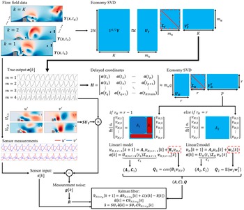
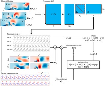
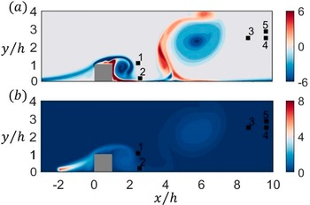
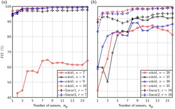


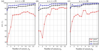


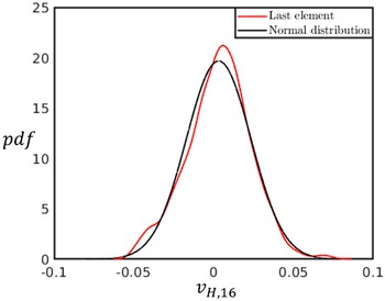

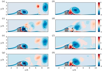


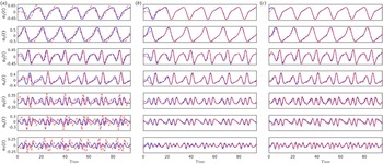


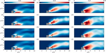


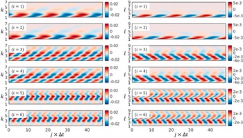


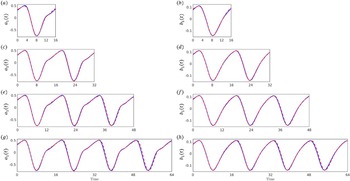


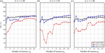


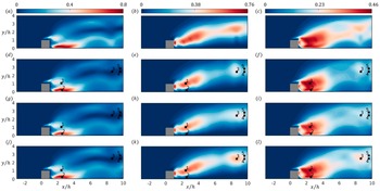


 Open access


Comments
No Comments have been published for this article.