2.2.1. Physical setting

There are many data fields that any model must use as boundary conditions to describe the physical setting of the ice sheet. The particular data fields of Greenland and Antarctica used as standards for the SeaRISE experiments are listed in Table 1, along with the source of each dataset. These datasets can be found at http://websrv.cs.umt.edu/isis/index.php/Data. Many of these datasets are leveraged off the effort of the Community Ice Sheet Model (CISM) that supplies gridded data associated with both the Greenland and Antarctic ice sheets (http://websrv.cs.umt.edu/isis/index.php/Main_Page).

Table 1. Datasets provided for use in initializing and running all SeaRISE experiments. Sources of each dataset are given. Data files and more details about them can be found at http://websrv.cs.umt.edu/isis/index.php/Data

SeaRISE’s desire for up-to-date versions of these parameter fields contributed to a broad effort to improve them with the most recent observations. Glaciologists around the world, some not directly involved in SeaRISE, contributed their most current data so that SeaRISE models could work with the best datasets. The Antarctic bed elevation was updated by a prerelease version of the updated BEDMAP dataset (courtesy of H. Pritchard) that included detailed new airborne radar data and new bathymetry in some offshore areas. This was further improved, as part of a separate modeling effort, by removing some unrealistic gridding artifacts, and the revised more ‘model-friendly’ data provided to SeaRISE modelers (Reference Le Brocq, Payne and VieliLe Brocq and others, 2010). In Greenland, the SeaRISE database includes new compilations of the bed topography that incorporate the subglacial troughs of Jakobshavn Isbræ as well as Helheim, Kangerdlussuaq and Petermann glaciers based on new radar data collected by the Center for Remote Sensing of Ice Sheets (CReSIS) and NASA’s IceBridge mission by employing an algorithm that maintains a deep trough even when that trough is narrower than the 5 km grid spacing (Reference Herzfeld, Wallin, Leuschen and PlummerHerzfeld and others, 2011). Use of better-defined outlet glacier troughs improves the realization of the surface flow field (Reference Herzfeld, Fastook, Greve, McDonald, Wallin and ChenHerzfeld and others, 2012).

2.2.2. Initialization (spin-up and tuning)

SeaRISE models initialize by ‘spinning up’, by ‘tuning’ or by a combination of the two. Both methods are designed to minimize differences between modeled and observed ice-sheet velocities and thickness distributions. These differences are created because required model parameters have inaccuracies caused by measurement errors, interpolations of sparsely sampled data, temporal mismatching and other sources. The initialized states often contain transients, i.e. the modeled ice sheet continues to evolve without any change in prescribed climates. As the model runs, these adjustments gradually decrease as the geometry, stress, temperature and motion fields approach equilibrium, but they can mask or influence the ice-sheet changes caused by a specific experiment’s prescriptions. All models express this effect to some degree, so, as described below, the impacts of any projected environmental change are calculated as a difference from an experiment where modern climate conditions are held constant.

‘Spin-up’ initialization refers to running the model through one or more glacial/interglacial cycles to reach internal consistency. It requires climatic information over hundreds of thousands of years. For SeaRISE models using this initialization approach, datasets of temperature derived from the ice cores were used: a 125 ka record from the GRIP ice core for Greenland and a 405 ka record from the Vostok ice core for Antarctica.

Initialization by ‘tuning’ refers to selecting a particular data field (or fields) as a target(s) and adjusting the independent variables of the model to come acceptably close (i.e. within a specified mismatch tolerance) to this target. Generally, geometry and environmental parameters are specified and the calculated velocity field is tuned through lubrication or strain enhancement factors to match the surface velocity (or balance velocity) field. Once tuned, these tuning parameters are usually held constant. Details of specific models are given in Table 2 and Appendix A.

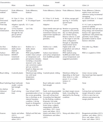
Table 2. Characteristics of models used in SeaRISE (additional capabilities of some models may not be indicated here if not used in SeaRISE experiments; details in Appendix A)

Table 2. Continued.

A goal of both types of initialization is to have the model output match reality in as many characteristics as possible at the time the experiment runs commence. The characteristics that are used as targets to match for SeaRISE models are the shape of the ice sheet (usually surface elevations or ice thickness over a static bed) and its surface flow field (see Reference NowickiNowicki and others, in press a, Reference Nowickib, for these spatial comparisons). Rates of change of either, or both, of these fields have been used in other modeling exercises but are not used by SeaRISE models. Whether ‘spinning up’ or ‘tuning’, SeaRISE set 1 January 2004 as the starting time of all experiments.

2.2.3. Experiments

As mentioned above, coupling of realistically dynamic ice-sheet models to predictive climate models is at a very early stage, and most ice-sheet models are only beginning to include poorly understood processes that are primarily responsible for recently observed dramatic flow accelerations/decelerations and rapid ice-thickness increases/decreases. Forcing ice-sheet models with environmental conditions computed by independent climate models may not provide credible projections of ice-sheet response if those ice-sheet models contain unrealistic dynamics. The modeling community continues to work toward the goal of ice-sheet models with improved dynamics fully coupled to global climate models, but its realization is many years away.

In light of this situation, SeaRISE designed a set of experiments wherein the effect of the environment is prescribed as a common forcing to each ice-sheet model. In basic terms, the environment interacts with the ice sheet on either its upper or lower boundary or at its perimeter. This holistic view drove the definition of the experiments where a change experienced by the ice sheet was imposed at one or more of these interfaces. The need to formulate standardized experiments, applicable to all or most models, strongly influenced their simple form. It is certainly possible to contemplate experiments that capture more realistic climatic and glaciological scenarios than those used in the SeaRISE experiments. In fact, SeaRISE participants considered many forms of such scenarios but rejected experiments that could not be consistently implemented for the majority of models, to preserve the project’s strength of using multiple models. In so doing, SeaRISE sacrifices some real-world complexity for the sake of increasing the number of models running each experiment. As such, these experiments represent more an attempt to measure ice-sheet sensitivity to specific forcing conditions rather than a coupled interaction of the ice sheet with the global climate. Most experiments ran 500 years into the future, thus covering the 200 year time focus of the next IPCC assessment report. The upper surface forcing uses calculated changes in atmospheric temperature and precipitation from the IPCC Fourth Assessment Report; the basal forcing amplifies basal sliding; and the perimeter forcing prescribes the melt rate beneath floating ice shelves. More details of each are given below when the specific experiment conditions and results are presented.

5.1.1. Surface climate experiment

The first set of external forcing experiments prescribes a set of changing climate conditions at the upper surface of the ice sheet. Changes in surface air temperature and precipitation were calculated by many global climate models for a number of climate scenarios included in AR4 of the IPCC and made available to the research community. The A1B scenario attempts to simulate rapid economic growth in a more integrated world with a balanced emphasis on all energy sources (Reference SolomonSolomon and others, 2007). It increases atmospheric CO₂ at slightly less than half the rate of the more fossil-fuel intensive A1F1 scenario. The calculated temperature and precipitation values of the A1B scenario for 18 models were combined into a time series of their monthly mean values and made available to SeaRISE (personal communication from T. Bracegirdle, 2009).

The IPCC model runs began in calendar year 1998 and lasted 100 years. SeaRISE runs begin in calendar year 2004, 6 years later, so these A1B fields apply for the first 94 years of SeaRISE model runs. The SeaRISE project reprojected these averaged A1B outputs onto the SeaRISE grids for Greenland and Antarctica and converted them to anomaly fields of temperature and precipitation for use in the SeaRISE climate-sensitivity experiments. These were then applied to whatever scheme each model used to calculate its grid of surface mass-balance values. Most, but not all, models used some form of ‘positive degree-day’ (PDD) scheme (see Table 2), but even these could vary in necessary scaling parameters, such as lapse rate. The ISSM and CISM-2 models used a simplified surface mass-balance scheme that did not discriminate between solid and liquid precipitation. This simplification would tend to overestimate mass accumulation, reducing mass loss.

Figure 2 illustrates the temporal pattern of these anomalies averaged over the entire Greenland or Antarctic ice sheet. The mean values in 2004 for Greenland are −18.63°C and 0.36 m w.e. a⁻¹ and for Antarctica are −35.53°C and 0.16 m a⁻¹. As expected in a warming climate, both temperature and precipitation increase.

Fig. 2. Anomalies of surface temperature and precipitation averaged over the Greenland and Antarctic ice sheets derived from 18 climate models submitted to the IPCC AR4 running the A1B forcing scenario.

These AR4-A1B scenario-based anomalies form the basis of the climate-forcing experiments. Prescribing them directly defines the first of these experiments (designated C1). Because the IPCC model runs were limited to 100 years and SeaRISE has a later starting date, these anomaly values could be applied for only 94 years. From year 95 to the end of the 500 year simulation, the conditions during year 94 are repeated. The final 6 years of Figure 2 illustrates the beginning of this extensive period of steady climate.

The two additional climate-sensitivity experiments (C2 and C3) amplify these temperature and climate anomalies by an additional 50% and 100%, respectively, i.e. C2 amplifies the A1B forcing by a factor of 1.5 and C3 prescribes temperature and precipitation anomalies twice as large as the A1B forcing.

Figure 3 presents the change in VAF of the SeaRISE model simulations of the C1, C2 and C3 experiments differenced from the control run to remove unrelated adjustments associated with initialization (as discussed earlier). There is a large spread in the response magnitudes, but all models project a decreasing VAF at all times in each experiment. For reference, a loss of 4.0 × 10¹⁴ m³ of ice (above flotation) equates to a 1 m rise in mean global sea level, and all plots (except Fig. 1) use a consistent VAF unit of 10¹⁴ m³. The IcIES and PISM models lose the most ice, reaching this 1 m sea-level contribution ∼350 years after the simulation begins for the doubled A1B scenario (C3). The ISSM model loses the least ice (for the models run for the full 500 years) and projects a sea-level contribution of only 8.5 cm after 500 years. The CISM-2 model was only run for 200 years, but projects losses less than half that of the ISSM model.

Fig. 3. Results of climate sensitivity experiments for the Greenland ice sheet. Upper panels show calculated change in VAF for the triplet of cases where prescribed temperature and precipitation changes are taken from the A1B scenarios of the IPCC AR4: left, C1, 100% of A1B changes applied; middle, C2, 150% of A1B changes applied; right, C3, 200% of A1B changes applied. The calculated Average includes AIF1a but ignores AIF2a. Lower panels illustrate the sensitivity of VAF change for the same experiments versus the amplification of the applied A1B climate changes at 100, 200 and 500 years after the simulation start. See Table 2 and Appendix A for descriptions of the various models. Note: all ice volume change plots in this paper use a consistent unit of 10¹⁴ m³ to facilitate comparisons between plots.

The relative behaviors of the models for each climate experiment are similar. The two models with the least VAF loss (ISSM and CISM-2) are exceptional in not using a PDD scheme to calculate surface melt (Table 2) and it is likely that their inclusion of rain in the surface mass accumulation underestimates the VAF loss. All other models use the prescribed precipitation anomalies in combination with some reference accumulation field and a calculation of surface melting using a PDD scheme driven by the prescribed temperature anomalies to determine the surface mass balance. However, the specific parameters used to translate the temperature change to a melt rate vary between models; this is the likely primary source of the spread of VAF change between models.

The rate of VAF loss increases for all models during the first 94 years, when the magnitude of these changes continues to increase (see Fig. 2). Afterward, the climate changes remain constant (at the final year-94 values) and each model transitions to a more gradual rate of ice loss that slowly decreases. It is important to emphasize that this implies that if the prescribed climate conditions continued to warm, as is the case in most models that project changes beyond 100 years for any realistic emissions scenario, then the projected rates of ice loss would be considerably larger than the cases presented here.

The comparison of model response to the A1B amplification factor (lower panels of Fig. 3) indicates a nearly linear response for those models with the smaller responses (CISM-2, ISSM and UMISM), but a nonlinear response for the larger responding models (IcIES and PISM). These response characteristics do not change significantly throughout the 500 year run. The linearity of the VAF change on the A1B amplification factor was examined statistically for every model at 100, 200 and 500 years. Indeed, CISM-2, ISSM and UMISM have R ² values of 0.999 or higher at 100 years, while the lowest R ² value of 0.88 occurred for the AIF1a model at 500 years. In general, the R ² values for any model gradually decreased with time. This final trend toward slightly less linearity is captured in the R ² values of the models’ average sensitivity that decreases from 0.95 to 0.93 to 0.91 at 100, 200 and 500 years, respectively.

The 100 year change in ice volume expected from the increase in precipitation (Fig. 2) is an increase of 3.7 × 10¹² m³, a relatively small volume given the calculated volumes of ice lost. All models lose ice volume during this time, so the combination of increased melting and increased discharge clearly outweighs the volume gained through increased accumulation. For these experiments, the lost volume can be due to either melting, a direct result of warmer temperatures at a given elevation or an indirect result of surfaces lowered to warmer elevations, or increased discharge, driven by increased surface slopes generated by the altered surface mass-balance pattern. To discern the relative magnitudes of these mass loss effects, surface mass balance (SMB) is calculated at each time-step for each model as the area integral over all gridcells that contain ice at that time. Discharge flux is calculated for each model as the difference between total volume change and the time-specific areal integral of surface mass balance. These SMB and discharge values for the C1 (1×A1B) experiments are then differenced from the control experiment values to produce anomalies of both SMB and discharge, and then the ratio of discharge flux anomaly to the total surface mass-balance anomaly is calculated and plotted in Figure 4.

Fig. 4. Ratio of discharge flux anomaly to surface mass-balance anomaly for the C1 (1×A1B) climate experiment of the Greenland ice sheet. Anomalies are calculated by differencing discharge flux and surface mass-balance values from the respective control experiments. For comparison, the equivalent ratios for the C3 (2×A1B) experiment for the IcIES and ISSM models are also shown as short-dashed lines.

This ratio has several diagnostic characteristics. Positive surface mass-balance anomalies add mass to the ice sheet relative to the control case while positive discharge is taken here as representing mass loss (i.e. increased discharge) relative to the control. In all the experiments considered here, the change in surface mass balance imposes a net mass loss on the ice sheet (compared to the control experiments), so the SMB anomaly is always negative and the interpretation of positive or negative ratios in Figure 4 is unambiguous. Positive anomaly ratios indicate ice is being added by changes in discharge flux (i.e. discharge flux is less in the experiment than in the control run) while it is removed by changes in surface mass balance. The relative contribution of discharge flux anomaly to SMB anomaly is larger the larger the ratio. For a ratio of unity, the two contributions are equal and the ice-sheet volume does not differ from the control run. Negative ratios indicate ice is being lost by changes in both the discharge flux and surface mass balance relative to the control run. The fact that the anomaly ratio never exceeds unity is consistent with the characteristic illustrated in Figure 3 that VAF always decreases for every model.

During the initial 94 year period when temperatures and precipitation are increasing (Fig. 2), the models exhibit a variety of behaviors; IcIES is the only model that generates an anomaly ratio lower than −1, indicating an increase in discharge flux anomaly exceeding the decrease in SMB anomaly, but many models exhibit negative ratios that signal increasing discharge flux relative to the control. Midway through this initial 94 year period, the ratio for each model is on a persistent trajectory toward a rather steady positive value that is preserved for the last few centuries of the experiment.

Figure 4 also contains the results of the C3 (2×A1B) case for the ISSM and IcIES models, representing the minimum and the maximum VAF responses, respectively (Fig. 3). Other models fall between these two end cases. There is very little difference in the ratios of the C1 and C3 cases for ISSM. On the other hand, the maximally responsive IcIES model exhibits a considerable difference, with anomaly ratios for the C3 case much lower than the ratios for the C1 experiment in the later centuries, indicating the equilibration to the larger climate changes takes much longer before the discharge flux adjusts to balance the lower SMB.

5.1.2. Basal sliding experiment

Sudden and large changes in ice flow velocity have been observed (e.g. Reference Rignot and KanagaratnamRignot and Kanagaratnam, 2006; Reference Howat, Smith, Joughin and ScambosHowat and others, 2008). These changes are inferred to be the result of changes in basal sliding likely caused by changes in the subglacial hydrologic environment (e.g. Reference Joughin, Tulaczyk, Fahnestock and KwokJoughin and others, 1996; Reference Zwally, Abdalati, Herring, Larson, Saba and SteffenZwally and others, 2002; Reference Joughin, Das, King, Smith, Howat and MoonJoughin and others, 2008). Their effect on the overall mass balance of the ice sheet is significant and, in some catchments, dominates the rate of volume change (Reference Howat, Smith, Joughin and ScambosHowat and others, 2008). Many active field studies are underway, but a process-level understanding is probably many years away.

This lack of understanding makes it difficult to incorporate these processes into current ice-sheet models, but the undisputed importance of basal sliding in regulating ice-sheet discharge through outlet glaciers forces all viable ice-sheet models to incorporate some means of calculating sometimes large basal sliding rates. Most models include a lubrication factor; however, changing this by a uniform value, say by halving its value, does not always result in a direct doubling of sliding velocity if solution of the sliding velocity involves non-local stresses

The experiment approach taken is to prescribe an increase of the sliding speed by a uniform factor. A trio of sliding experiments set the sliding speed amplification factors as 2×, 2.5× and 3× for experiments S1, S2 and S3, respectively. Models that employ only local stresses to calculate the basal sliding velocity (IcIES, UMISM, SICOPOLIS and AIF) will maintain this enhanced sliding ratio, but those that use a more complex relationship utilizing both local and regional stresses (e.g. ISSM, PISM, Elmer/Ice and CISM-2) will experience sliding ratios that vary from the prescribed ratio; however, the deviations are generally not large. Figure 5 illustrates the results of model runs for this sliding experiment applied to Greenland.

Fig. 5. Results of basal sliding sensitivity experiments for the Greenland ice sheet. Upper panels show calculated change of VAF for the triplet of cases where basal sliding was increased by a constant factor: left, S1, 2×; middle, S2, 2.5×; right, S3, 3×. Lower panels illustrate the sensitivity of ice loss versus the basal sliding amplification factor at 100, 200 and 500 years after the simulation start. The calculated Average includes AIF1a but ignores AIF2a.

As with the previous set of (climate) experiments, there is a wide range of responses across the different models, but, overall, response magnitudes are not as large as for the set of climate experiments. All models show a gradually decreasing rate of VAF loss over time. The two versions of the AIF model predict larger ice losses when the basal sliding is an exponential function of the basal stress (version AIF1a) as compared to the linear function (AIF2a). The rough response character of the UMISM model is due to details of its treatment of retreat of the ice edge across gridpoints. The largest response is predicted by Elmer/Ice, the only SeaRISE model that incorporates full-Stokes dynamics (i.e. including bridging stresses in addition to longitudinal, lateral and vertical shear), but this model was only run for 200 years and the nature of the model’s internal composition resulted in sliding amplifications larger than specified. The shorter duration of Elmer/Ice and CISM-2 runs causes the kink at 200 years in the model-Average line in Figure 5. ISSM, using a higher-order set of equations (i.e. including longitudinal, vertical-shear and lateral-shear stresses), predicts the largest ice losses beyond 300 years.

The eight-model average response for experiment S1 at 100 years is a VAF loss of 2.73 × 10¹⁴ m³ which converts to an equivalent sea-level rise of 6.8 cm. This is comparable to the estimate of a 9.3 cm sea-level contribution by Reference Pfeffer, Harper and O’NeelPfeffer and others (2008) (table 3 and supplementary online material) when the discharge of 33 outlet glaciers was doubled. Their calculation included total volume lost, while ours is limited to the VAF, but, as mentioned earlier, the differences between total volume lost and VAF losses is small for Greenland.

Table 3. Global sea-level increase (cm) projected by SeaRISE models for each experiment at 100, 200 and 500 years since model initial time of 1 January 2004

In a manner similar to the climate experiments, the lower panels of Figure 5 show that the response sensitivity to the amplification of basal sliding after 100 years is more linear the smaller the response, tending toward a slightly nonlinear sensitivity for models with larger responses. At 100 years, the R ₂ values of linear fits of VAF loss sensitivity to the sliding amplification factor are all 0.99 or above except for Elmer/Ice (R ² = 0.98). At 200 years, only Elmer/Ice has a perceptible nonlinear sensitivity (although the R ² value is still 0.99) and at 500 years (without Elmer/Ice) all models retain R ² values above 0.98, demonstrating the strong linear sensitivity of VAF loss to the basal sliding amplification factor.

5.1.3. Ice-shelf melting experiment

The observed spatial pattern of recent ice-sheet changes has been interpreted as suggesting that increased melting at the underside of the fringing ice shelves and floating tongues of outlet glaciers is a key trigger of these changes (Reference Payne, Vieli, Shepherd, Wingham and RignotPayne and others, 2004; Reference Shepherd, Wingham and RignotShepherd and others, 2004; Reference Holland, Thomas, de Young, Ribergaard and LyberthHolland and others, 2008; Reference Joughin, Smith, Howat, Scambos and MoonJoughin and others, 2010). Again, very few whole ice-sheet models incorporate an oceanographic component enabling ocean/ice interaction in a fully coupled manner. Nevertheless, the importance of this interaction led SeaRISE to generate a third set of experiments to gauge the sensitivity of the ice sheets to basal melt rates beneath floating ice.

As with basal sliding calculations, model variation constrained the realism in how this type of experiment could be implemented. PISM has no floating ice at the end of its Greenland spin-up, and melting was not imposed on the tidewater margin of the outlet glaciers, so it was unable to provide meaningful results for this experiment. For similar reasons, Elmer/Ice and CISM-2 were not able to perform the ice-shelf melting experiments. Of the remaining models, only one (ISSM) included ice shelves, but the boundary between the grounded and floating ice remains fixed; the others (IcIES, SICOPOLIS, UMISM and AIF) opt to ignore any ice that floats and apply the basal melt rates at the ocean boundary of grounded ice. The concentration of the prescribed melt rate at the grounding line is a reasonable approximation given the inference that basal melt rates are generally highest near the grounding lines (Reference Williams, Grosfeld, Warner, Gerdes and DetermannWilliams and others, 2001; Reference Payne, Holland, Shepherd, Rutt, Jenkins and JoughinPayne and others, 2007). The three SeaRISE experiments in this category set the submarine melt rate at uniform values of 2, 20 and 200 m a⁻¹ for experiments M1, M2 and M3, respectively. The results of these experiments (again minus the effects of the control runs) are shown in Figure 6.

Fig. 6. Results of ocean melting sensitivity experiments for the Greenland ice sheet. Upper panels show calculated ice loss for the triplet of cases where ocean melting was set to constant values: left, M1, 2 m a⁻¹; middle, M2, 20 m a⁻¹; right, M3, 200 m a⁻¹. Lower panels illustrate the sensitivity of ice loss vs the three different melt rates at 100, 200 and 500 years after the simulation start. The calculated Average includes only AIF1a and ignores AIF1b, 2a and 2b.

The range of projected ice loss for these basal melt experiments is larger than for either the climate or basal sliding experiment suites, but much of the variation can be explained by the manner in which the basal melt rates were applied. The most responsive models in all three experiments are the 1b and 2b versions of the AIF model which apply the melt rate along the entire ice-sheet perimeter. This is clearly so unrealistic that these results are not included in the calculated Average. Despite the extreme nature of this assumption, they are useful when interpreted in tandem with the ‘a’ scenarios of the AIF model as bracketing the magnitude of Greenland’s ocean/ice interaction. The other useful pair of end points is the UMISM and ISSM models. The ISSM model includes ice shelves, but imposes the melt rate only at the front and maintains that front position until melting has removed all the ice there, only then retreating the ice front to the next gridpoint upstream. No melting is ever imposed to initially grounded ice, so no further melting occurs once the ice margin retreats beyond this boundary, severely limiting the ice loss for this suite of experiments. UMISM includes the dynamic effect of ice shelves by imposing a back-stress on the grounded ice according to theoretical formulations (Reference ThomasThomas, 1973) and a large thinning rate at the grounding line according to Reference WeertmanWeertman (1974). This thinning rate leads to rapid inland erosion of the ice sheet along coastal fjords drawing down the ice within the catchments of marine-based outlet glaciers. The results from the other models fall between the two extremes set by both the AIF ‘a’ vs ‘b’ versions, ISSM and UMISM. It is possible that the VAF loss for all models is exaggerated by the fact that the 5 km grid resolution effectively sets a too-large minimum width for many narrow fjords, causing excessive ice loss. Despite the significant approximations these models use to treat this difficult boundary, they are among the best models available at present, and their combined results may be the best approximation of the sensitivity of the ice sheet to basal ice-shelf melting.

An additional insight provided by the extreme case of 200 m a⁻¹ is that it provides a trajectory of decreasing VAF that helps determine the ice sheet’s ultimate vulnerability to oceanic erosion. Because ice loss is continuing even after 500 years, the ocean’s effect on the ice sheet is not short-lived. Even after the floating edge of the ice sheet is removed, increased drainage of ice into the ocean will continue for centuries. Extrapolating the Average trajectory many centuries beyond the end of the 500 year experiments, the eventual volume of ice above flotation lost is likely at least 2 × 10¹⁴ m³, or 50 cm of globally averaged sea level.

The widely ranging nature of model responses to the strength of melt rate is also expressed in the sensitivity plots of Figure 6. The VAF changes at 100, 200 and 500 years are plotted on a log scale of the imposed melt rate, making the strength of a linear relation difficult to visualize. At 100 years, IcIES and SICOPOLIS have R ²>0.99; AIF1a and 2a have linear fits with R ² near 0.9, decreasing to near 0.7 for UMISM and ISSM. By 500 years, IcIES and SICOPOLIS maintain their linear character with R ²>0.99; AIF1a and 2a have decreased to the overall minimum R ² values of 0.36 and 0.47, respectively, while UMISM and ISSM have R ₂ values of 0.58 and 0.74, respectively. The sublinear sensitivity of UMISM (Fig. 6) is probably due to the absence of additional ice available to be removed in the extreme (M3) experiment that was not already removed in the intermediate (M2) experiment.

5.1.4. Combination experiment

Each of the above experiments isolates a particular forcing type at prescribed values to measure the sensitivity of the modeled ice sheet to that single forcing. In reality, however, multiple forcings are expected to act simultaneously and it cannot be assumed that these separate sensitivities are additive in determining the total sensitivity to a combination of environmental changes. To examine this subject, a combination experiment was specified which simultaneously imposes the 1×A1B climate change (C1) with the 2× sliding velocity changes (S1) for Greenland. No additional forcing related to the floating-ice melting experiment suite was included, because the implementation of this forcing varied the most across all models.

The results of this combination experiment, labeled C1S1, are shown in Figure 7a. The temporal pattern noted in the C1 experiment, of an increasing rate of ice volume loss over the first 94 years, followed by a gradually decreasing rate of ice loss, is repeated for nearly all models, but is more subdued, presumably because the S1 experiment lacked a transition at year 94. The only exception is the Elmer/Ice model that fails to show a transition at year 94 in the combination experiment, but Figures 3 and 5 show this model’s response to the S1 basal sliding forcing is more than four times stronger than its response to the C1 climate forcing, so this absence of a change in the trend of VAF loss at 94 years is not surprising.

Fig. 7. Results of experiment for Greenland combining the C1 and S1 forcings. (a) Projected change in VAF; (b) the ratio of the VAF loss for the C1S1 combination run divided by the sum of the VAF losses for the C1 and S1 experiments.

The issue of how well the sum of the two individual responses matches the response when the two forcings are prescribed in the same experiment is illustrated in Figure 7b. This plot shows the ratio of the VAF lost in the combination experiment to the sum of the VAF lost separately in the C1 and S1 experiments. In all cases, this ratio is close to unity. This is true whether the model is more sensitive to the climate experiment than the sliding experiment (like PISM and IcIES) or the reverse (like Elmer/Ice and SICOPOLIS). Some models exhibit ratio values less than 1, indicating the combination run experienced less VAF loss than the sum of the C1 and S1 runs. This is likely due to the fact that some parcels of ice were lost in both the C1 and S1 runs but could only be lost once in the combination run. Other models exhibit ratios greater than 1, indicating an amplified response of the combination experiment where one type of forcing increases the response to the second forcing. One example of how this might manifest is that the A1B climate induces a steeper surface slope that increases basal shear stress and, thus, sliding velocity, which is then amplified by the S1 forcing conditions of doubled basal sliding and delivers more ice either to lower elevations, where it is melted, or to the margins, where it calves into the ocean. These ratios are not constant in time, but are generally stable, lying within +5% of unity. PISM is the only model whose ratio continues to increase over the latter half of the experiment, but even it begins to stabilize in the last 150 years. The discovery that linear combinations of individual forcings closely approximate the response of an experiment that applies these forcings simultaneously is significant and is explored further below.

5.1.5. Summary

Ten experiments spanning a wide range of prescribed environmental changes have been run by many models that simulate the dynamics of the Greenland ice sheet. In general, the calculated responses illustrate similar behavior but with a range of response magnitudes. Figure 8 includes the model-Average response from each experiment on a common scale to better compare the relative response magnitudes to the different types and magnitudes of forcing. The smallest changes are produced by the M1 (2 m a⁻¹) basal melting experiment. The more modest forcings of climate (C1) and basal sliding (S1) produce similar temporal patterns of VAF loss, with their combination (C1S1) doubling the net losses of either individually.

Fig. 8. Results of average response for models for each Greenland experiment. Each suite of experiments is shown in a common color, with the mildest, intermediate and extreme experiments represented by a solid, dashed and dotted line, respectively. A kink appears in the climate, sliding and combination results because the Elmer/Ice and CISM-2 runs only lasted 200 years. There is no kink in the melt experiments; neither Elmer/Ice nor CISM-2 ran the melting experiments.

The largest range of model-Average response occurs for the climate experiment trio, with C3 (2×A1B) producing the largest VAF losses, although the most extreme melt experiment M3 (200 m a⁻¹) produces the largest initial VAF losses. The suite of experiments with the smallest range of response is that which varied the amplification of basal sliding; however, the full magnitude of this sensitivity may be limited by the models’ abilities to adequately represent the basal sliding in narrow outlet glacier fjords.

These results suggest some fundamental characteristics of the Greenland ice sheet’s volumetric response to environmental changes. The fastest response can be driven by a sudden and large change to the basal melt rate at the ocean/ice interface; however, the intense initial response lasts only a few decades as the most vulnerable ice is removed, after which the rate of ice loss decreases markedly. Changes in climate (here represented by surface temperature and precipitation changes) can also have a large effect on ice-volume loss, but these losses are achieved through a sustained adjustment of the ice sheet to the altered climate that lasts centuries (and even millennia). The range of climate changes covered in these experiments is arguably more realistic than either the range of basal sliding or ice-shelf melting experiments. To be more realistic, the enhanced sliding may need to be localized to apply more strongly near the outlet glaciers; however, our results do compare well with those of Reference Pfeffer, Harper and O’NeelPfeffer and others (2008), as discussed earlier. Association of basal sliding with surface melt also might improve realism, yet observations of surface lake drainage and ice-flow response underscore the as-yet mysterious nature of basal sliding dynamics (Reference DasDas and others, 2008; Reference Joughin, Das, King, Smith, Howat and MoonJoughin and others, 2008). More promising is the result that despite the relatively large changes in basal sliding imposed, the range of ice-sheet response is limited. Similar model improvements are required for better simulation of the effects of ice-shelf melt rates on the ice sheet.

5.2.1. Surface climate experiment

There is no change to the nature of climate-forcing experiments: C1, C2 and C3 refer to the ensemble mean AR4 A1B changes in temperature and precipitation being imposed for 94 years with amplification factors of 1, 1.5 and 2, respectively, and being held at the year-94 values for the remainder of the 500 year run (Section 5.1.1). The results of the six Antarctic models running these experiments are shown in Figure 9.

Fig. 9. Change of VAF for the climate sensitivity experiments of the Antarctic ice sheet. Upper panels show calculated VAF change for the triplet of cases where prescribed temperature and precipitation changes are taken from the A1B scenarios of the IPCC AR4: left, C1, 100% of A1B changes applied; middle, C2, 150% of A1B changes applied; right, C3, 200% of A1B changes applied. Lower panels illustrate the sensitivity of VAF change for the same experiments vs the amplification of the applied climate changes at 100, 200 and 500 years after the simulation start. Orange circles indicate the VAF change resulting only from the applied change in precipitation at 100, 200 and 500 years. See Table 2 and Appendix A for descriptions of the various models.

As with the Greenland experiments, there is a range of model responses. However, in the case of Antarctica, this range includes projections of increasing VAF, as well as VAF loss, although even for those models that project an overall increase in VAF, there is an initial loss of VAF in the first few decades. Antarctica’s ice-sheet area is ten times that of Greenland and the mean temperature is lower, so, unlike in the case of Greenland, increased precipitation has a larger integral effect that is not necessarily offset by rising temperatures increasing both the amount and extent of surface melting.

The additional volume derived exclusively from the increased precipitation can be calculated and is included in Figure 9 as orange circles. Over the first 100 years this additional volume is 1.33 × 10¹³ m³, a significant amount relative to the total changes predicted by the 1×A1B experiment (C1). The ISSM, AIF and Potsdam models predict a VAF change very close to this amount during the first 100 years; it is only in the later centuries that the dynamic response to the climate changes begins to offset an increasing proportion of this additional volume. (A cautionary note is warranted: because only the VAF is reported here, volume loss on ice shelves and much of the ice lost within deep marine basins, both of which are substantially more extensive in Antarctica than in Greenland, are not included; thus, there may be net ice-sheet volume loss even as VAF increases. Because the ice shelves are at the margins where many of the changes are strongest and first felt, while the deeper marine basins are affected later, it is reasonable to expect a more complex response evolution to the Antarctic experiments than shown in these figures that provide only VAF values; see Reference NowickiNowicki and others, in press a, Reference Nowickib, for more spatial details.)

The behavior of the other models is more varied: the PennState3D model increases VAF for two centuries before reversing to a decreasing VAF trend. The UMISM model shows only a very brief increase in VAF and then a decrease, and the SICOPOLIS model produces a more continuously decreasing VAF. This variety implies a complex combination of adjustments including not only the increased precipitation, but melting at the margins and the dynamic adjustments involving not only geometric changes, but interaction of the grounded ice with the ice shelves. The model-Average gradually and monotonically gains VAF.

The temporal pattern of adjustment to these changes, although varied by model, remains consistent for any model regardless of the strength of the climate forcing, i.e. all three panels in the upper row are nearly identical although the magnitude of the response increases with the strength of the forcing. The lower panels of Figure 9 suggest a high degree of linearity of the modeled VAF change to the magnitude of the prescribed forcing. A linear fit to each of these sensitivity plots bears this out: the R ² of fits to the AIF, Potsdam, UMISM and ISSM results are always >0.99. The R ² for the SICOPOLIS model increases from 0.56 at 100 years to 0.89 at 500 years, while the R ² for the PennState3D model decreases from 0.90 at 100 years to 0.80 at 500 years.

5.2.2. Basal sliding experiment

As in Greenland, the Antarctic ice sheet is drained by many large outlet glaciers with high rates of basal sliding, so the same suite of experiments is used to study the sensitivity of the Antarctic ice sheet to a uniform increase of basal sliding as was used for the Greenland experiments, i.e. the sliding velocity is amplified by 2, 2.5 and 3 for experiments S1, S2 and S3, respectively. It is important to repeat the caveat that not all models calculate sliding velocity in a way that ensures that sliding is enhanced by precisely these amplification factors. Those Antarctic models that do not are Potsdam and ISSM. As an example of the range of sliding amplifications that resulted, for experiment S2 (doubled sliding), ISSM produced sliding velocities that were very close to the desired doubling for most of the ice sheet, but the ratio of altered sliding speed to non-altered sliding deviated from a low of 1.7 to a high of 2.3.

While many of the Antarctic outlet glaciers and ice streams are larger than their Greenland counterparts, so are the total ice-covered area and ice volume. To counter the increased computational demands of the larger domain, the Antarctic models typically use a coarser spatial resolution that is often twice the grid dimension used in Greenland, so the limitations encountered with being able to spatially resolve the dynamic response of outlet glaciers are just as severe. This constraint will only be overcome with finer spatial meshes, nested grids and/or the application of regional models (e.g. Parizek and others, in press).

Figure 10 shows the results from the suite of basal sliding enhancement experiments for Antarctica. In this case, all models lose ice volume above flotation. The temporal pattern of loss among the models is similar while the magnitude of VAF loss increases with sliding amplification. Most models exhibit a decreasing rate of loss with time. The ISSM model stands out as losing VAF at a very nearly constant rate for the entire experiment, thus diverging from the other models at an increasing rate over the latter half of the simulation.

Fig. 10. Results of change in VAF for the basal sliding sensitivity experiments of the Antarctic ice sheet. Upper panels show calculated VAF loss for the triplet of cases where basal sliding was increased by a constant factor: left, S1, 2×; middle, S2, 2.5×; right, S3, 3×. Lower panels illustrate the sensitivity of VAF loss vs the basal sliding amplification factor at 100, 200 and 500 years after the simulation start.

The sensitivity of VAF change can be approximated with a least-squares linear fit with R ² values above 0.92 for all models at all three epochs shown in Figure 10 except for the UMISM model. UMISM shows a consistent reverse sensitivity. This might be due to the locations where ice is being lost: as deep marine basins empty, the initial thinning counts as VAF loss, while once the ice thickness reaches the flotation thickness, subsequent ice loss will not add to the values shown in Figure 10. Furthermore, initial thinning and flattening of the ice sheet reduces the local driving stress and therefore outflow, thereby contributing to UMISM’s reversed sensitivity. SICOPOLIS’s nonlinear sensitivities are not as strong, and overall the model-Average sensitivity has an R ² of 0.98 for all times shown in Figure 10.

5.2.3. Ice-shelf melting experiment

The largest observed changes in Antarctic mass loss are associated with changes in its fringing ice shelves (e.g. Reference Scambos, Bohlander, Shuman and SkvarcaScambos and others, 2004; Reference Shepherd, Wingham and RignotShepherd and others, 2004; Reference Pritchard, Ligtenberg, Fricker, Vaughan, Van den Broeke and PadmanPritchard and others, 2012). Thus, this suite of experiments aimed at examining the possible sensitivity of the Antarctic ice sheet to basal melt of floating ice is particularly germane. Again, repeating the Greenland experiments, the three experiments in this suite set the bottom melt rate for floating ice at uniform values of 2, 20 and 200 m a⁻¹. Figure 11 shows the results of the experiments.

Fig. 11. Results of change in VAF for the ocean melting sensitivity experiments of the Antarctic ice sheet. Upper panels show calculated VAF loss for the triplet of cases where ocean melting was set to constant values: left, M1, 2 m a⁻¹; middle, M2, 20 m a⁻¹; right, M3, 200 m a⁻¹. Lower panels illustrate the sensitivity of VAF loss vs the three different melt rates at 100, 200 and 500 years after the simulation start.

As discussed earlier (Section 5.1.3. and shown in Table 2), there is a variety of approaches to how the ice shelves are treated in the models. Of the Antarctic models, SICOPOLIS, PennState3D and Potsdam include ice shelves. AIF and UMISM do not include ice shelves, instead applying the melt rate at the grounding line, but UMISM does incorporate both a back-stress and a longitudinal thinning rate at the grounding line to include dynamic effects of the ice shelf. Figure 11 shows that, despite these differences, all models lose VAF when the basal melt of floating ice is increased, even though the direct loss of ice-shelf mass does not appear in the plotted VAF values. Arguably, at 100 and 200 years the scatter among models is less than the same times for the Greenland ice-sheet models (Fig. 6) despite the much larger size of the Antarctic ice sheet. However, unlike the other experiment results for either ice sheet, the relative responses of the models vary significantly more among these three basal melting experiments. For the mildest melt case (M1), the PennState3D model reacts most strongly, while the AIF, SICOPOLIS and UMISM models form a very tight cluster. For the intermediate melt case (M2), the UMISM model is generally consistent with the PennState3D model while the Potsdam and AIF models are also consistent with each other. Finally, in the extreme melt case (M3), the UMISM model produces much higher VAF losses than any other model, and consistent pairs of models are less apparent.

The large experiment-to-experiment variability is understandable given the knowledge that large volumes of floating ice shelves are being rapidly removed along with the evacuation of extensive deep marine basins in the M2 and M3 experiments. As one example of how this affects the results shown in Figure 11, the seemingly modest increase in VAF lost for the PennState3D model from the M2 to the M3 experiment is caused by the fact that most of the marine-based West Antarctic ice sheet is already lost in the M2 experiment; higher melt rates also remove this same ice but only a relatively small amount of additional ice in East Antarctica, an ice sheet less vulnerable to ice-shelf loss. By contrast, the UMISM model, because it applies the prescribed melt rates to the edge of the grounded ice, can erode the edge of the East Antarctic ice sheet, and the very large VAF losses for its M3 experiment reflect the loss of ice in deep marine basins there.

Because only changes in the volume above flotation are reported, the results are influenced by how each model handles the migration of the grounding line. The Penn-State3D model is the only one that fully employs the transitional stress treatment of Reference SchoofSchoof (2007), yet the relative agreement of the models suggests that the details of grounding line migration may be less important than developing means to accurately determine basal melt rates beneath the ice shelves.

The sensitivity diagrams (Fig. 11, lower panels) emphasize the extreme VAF lost in many of the models for the largest basal melt rates. The linearity of the fits is difficult to discern from the log scale. At 100 years, the UMISM, Potsdam and AIF models have R ² values of 0.99 or higher, SICOPOLIS is lower with R ² = 0.81, and R ² for PennState3D is 0.70. These relative positions are approximately retained at 500 years, with USISM and Potsdam remaining above 0.99, but the other values have decreased to 0.79, 0.67 and 0.43 for AIF, SICOPOLIS and PennState3D, respectively.

5.2.4. Combination experiments

For the Antarctic, three combination experiments are defined. Each included the A1B climate forcing without amplification (C1). The first experiment added 2 m a⁻¹ basal melting of ice-shelf ice (M1) to the climate forcing. The second experiment added doubled basal sliding (S1) to the climate forcing (identical to the Greenland combination run). The final combination run added both doubled sliding (S1) and a more ablative 20 m a⁻¹ ice-shelf basal melt (M2) to the A1B forcing. The labels assigned to each experiment (C1M1, C1S1 and C1S1M2) indicate the forcing scenarios that were combined.

The results of these combination experiments are shown in Figure 12 in which we plot the temporal records of VAF change as well as the ratio of the VAF change from the combination run to the sum of VAF changes for the separate components making up the combination. All combination experiments show progressive VAF losses for all models.

Fig. 12. Results of the three combination experiments of the Antarctic ice sheet: left, A1B climate forcing (C1) combined with 2 m a⁻¹ ice-shelf basal melt rate (M1); middle, A1B climate (C1) combined with doubled sliding (S1); right, the triple combination of A1B climate (C1), doubled sliding (S1) and 20 m a⁻¹ ice-shelf basal melting (M2). Upper plots show calculated change in VAF while the lower plots show the ratio of these VAF losses for the combination run divided by the sum of the VAF losses for the individual component runs.

In the first experiment (C1M1) the modest melt rate is sufficient to cause net VAF loss for the AIF model, but does not eliminate the Potsdam model’s VAF growth in the first two and a half centuries predicted for the C1 experiment alone. M1 forces a stronger response than C1 for most models, and the results of this combination experiment are close to the sum of C1 and M1, i.e. the ratio of the combination to the sum of the individual runs is close to unity, with this tendency toward unity being particularly strong later in the runs. The Potsdam model shows considerable temporal variability of the VAF ratio, probably because the timing of regional ice loss varies between the individual runs and the combination experiment. UMISM and, to a lesser degree, SICOPOLIS also show some strong temporal variability of this ratio during the first few decades.

The second combination experiment (C1S1) combines doubled basal sliding (S1) with the A1B climate changes (C1). All models again persistently lose VAF. The spread of VAF loss across models is almost identical to that of the C1M1 combination experiment, but the rates of VAF loss for most models decrease with time, rather than increase as in the C1M1 experiment. The ratios of the combination response to the sum of the individual experiments show temporal variability for some models but with smaller magnitudes than in the C1M1 experiment. Some models have ratio values consistently less than unity, and fewer models converge on unity. A ratio less than unity indicates a weaker combined response than the sum of the individual responses. The tendency of an increasing ratio for the PennState3D model tends to offset the decreasing tendency of the ratio for the SICOPOLIS model, producing an Average result that remains relatively stable.

The third combination experiment (C1S1M2) adds the intermediate ice-shelf basal melt rate of 20 m a⁻¹ (M2) to both the doubled basal sliding (S1) and A1B climate changes (C1). The responses among all models are noticeably more consistent than in the other combined experiments, with all producing significant VAF losses at a rate that decreases with time. Considered individually, the melting produces the largest response of these three forcings, and even when combined with the S1 and C1 forcings all models show VAF losses that are very similar to the M2 case alone (Fig. 11, middle top panel). The SICOPOLIS model exhibits the largest difference between this combination experiment and the M2 experiment, so it is not surprising that the ratio values of the combination results to the linear sum of the individual experiments for this model are largest (Fig. 12, lower right panel). The temporal patterns of this ratio show a larger VAF loss in the combination run initially which in the SICOPOLIS and AIF models persists for the entire 500 years, but for the UMISM and PennState3D models this larger response is shorter-lived. The Potsdam model exhibits the opposite tendency: a ratio less than unity early in the experiment, growing to values above unity and increasing as time increases. Ratios above unity could well be due to enhanced sliding delivering more ice to the ice shelves where it is rapidly removed through the higher prescribed melt rates. Such an evolution is seen in regional SeaRISE results for Thwaites Glacier (Parizek and others, in press).

The overall conclusion of these three combination experiments is that these forcings produce little, if any, enhancement of VAF loss when they are applied simultaneously. Only in the final experiment (C1S1M2) do the ratios in the SICOPOLIS, Potsdam and AIF models persist well above unity; the other two models (UMISM and PennState3D) display no such enhancement. Indeed, the ratio of these latter models is less than unity, as is SICOPOLIS for the second combination experiment (C1S1) and many models in the first combination experiment (C1M1).

5.2.5. Summary

The temporal changes in ice volume above flotation averaged across all the models for each experiment are plotted on a common scale in Figure 13 to assess the relative responses. There are many differences compared to Greenland (Fig. 8), with the largest arguably being that the climate-forcing experiments all cause the model-Average response for Antarctica to be an increase in the VAF. The average growth, however, is less than the average VAF loss for Greenland under similar forcing.

Fig. 13. Results of model-Average VAF change for all Antarctic experiments. Each suite of experiments is shown in a common color, with the mildest, intermediate and extreme experiments represented by a solid, dashed and dotted line, respectively. The average value of the M3 experiments is −34.5 × 10¹⁴ m³ at 500 years.

For Antarctica, the climate-forcing experiments produce the weakest response, slightly negative in the early decades, reversing to slight VAF gain throughout the remainder of the 500 years. The strongest response is to experiments prescribing the intermediate and extreme increase to the basal melting of ice shelves. For some models without explicit ice shelves, the increased melt rate is imposed at the edge of ice sitting in the ocean. The VAF losses for these strongest response experiments vastly exceed those calculated for the Greenland ice sheet. This is not surprising given the large areal extent of Antarctic ice shelves into which most major outlets discharge. Because the VAF is not affected by loss of ice shelves and less affected by the loss of ice sitting in deep marine basins, it is the inland propagation of thinning triggered and driven by these large melt rates that generates the large losses of VAF.

The magnitudes of changes in VAF for the sliding amplification experiments lie between the average gains of the climate experiments and losses of the melting experiments and are roughly three times larger than those for the sliding experiments for Greenland (Fig. 8).

The VAF lost in the melting and sliding experiments is so much larger than the growth of the climate experiments that net VAF loss is predicted in each of the three combination experiments. Figure 13 strongly suggests that this would be true had even the most extreme of the climate scenarios (C3:2×A1B) been used.

The fact that the responses of single-forcing experiments provide a close approximation to the response of the associated combination experiment was discussed in Section 5.2.4 and illustrated in Figure 12. This similarity also holds for the model-Average responses and can be seen in Figure 13: for example, by noting that temporal pattern of increasing ice loss for C1S1M2 in Figure 13 lies beneath the M2 curve by an amount very nearly equal to the sum of the S1 and C1 curves.

6.2.1. Climate conditions

The connection between the RCPs and the SeaRISE forcings is made through atmospheric temperature and IPCC AR4 scenarios. SeaRISE developed its climate-forcing experiments (C1, C2 and C3) from the A1B scenario of the IPCC AR4 (see Section 5.1.1). The AR4 scenario A2 is more extreme than A1B and most similar to RCP8.5 of the new scenarios, so scenario A2 is used as a proxy for RCP8.5. Based on the IPCC models of the AR4, by 2100 both the Arctic and Antarctic warm ∼50% more in the A2 scenario than in the A1B scenario. Thus, we take the first-century SeaRISE forcing for the R8 experiment as 1.5×A1B (the beginning of the C2 experiment). For the second century, Figure 14 indicates the radiative forcing increase for 2100–2200 is about half of the increase from 2000 to 2100. We chose to repeat the 1.5×A1B forcing through this century (rather than reduce it to 1/2×1.5×A1B) to capture some of the delayed warming from the first century’s radiative input that will occur during the second century. For the final three centuries of the 500 year run, RCP8.5 is flat (Fig. 14), but modest delayed warming from the second century’s radiative forcing increase is included by gradually increasing the temperature another modest increment.

For Greenland, the mean temperature increase in A1B over the final 10 years is 3.5°C (Fig. 2), so this final SeaRISE experiment imposes a 5.25°C increase in temperature in the first century, another 5.25°C increase in the second century, concluding with a final 0.75°C increase over the final 300 years for a total of 11.25°C. The temporal profile of the warming for the R8 experiment is illustrated in Figure 14, superimposed on the RCP8.5 profile of radiative forcing. It is also worth noting that Figure 14 shows that experiment C1 roughly approximates RCP6, with only a slight underestimate of forcing after 2100.

For Antarctica, the mean temperature increase in A1B is 2.29°C over the final 10 years (Fig. 2), so a 3.4°C increase in temperature (i.e. 1.5×A1B) is imposed in the first century of experiment R8, followed by another 3.4°C increase in the second century. The final 300 years of the experiment includes an additional temperature increase of 0.5°C: less than the gradual 0.75°C applied to Greenland but consistent with Antarctica’s reduced temperature increases during the first two centuries. The resulting total temperature increase for Antarctica is 7.4°C.

Amplification factors to apply to the A1B record of temperatures (Fig. 2) were calculated to prescribe this forcing for all SeaRISE models. The same amplification factors were used to modify the A1B precipitation values for the R8 experiment.

6.2.2. Basal sliding conditions

Changes in basal sliding are also expected to occur as part of the RCP8.5 scenario because there is an observed link between changes in surface meltwater penetrating the Greenland ice sheet and ice flow speed (Reference Zwally, Abdalati, Herring, Larson, Saba and SteffenZwally and others, 2002; Reference Joughin, Das, King, Smith, Howat and MoonJoughin and others, 2008). A quantifiable relationship between surface changes and basal speed, however, is not firmly established. In advance of a time when global climate model output can prescribe such changes in basal sliding, a rather ad hoc forcing is used drawing from the nature of the basal sliding sensitivity experiments already completed and described earlier. Basal sliding for Greenland is prescribed by setting the sliding amplification to a factor of 1.5, i.e. halfway between the control experiment (CC) and the doubled-sliding experiment (S1). This amplification remains constant for the entire R8 experiment.

For Antarctica, the basal sliding prescription is more complex. No sliding amplification is applied for the first century to incorporate the observation that there is, as yet, no warming-triggered acceleration of Antarctic outlet glaciers. After 100 years, the sliding is increased linearly at a rate of 20% of its original value per century, but only in the coastal regions because enhanced sliding due to melting from higher temperatures is expected to occur there first. Thus, at the coast, the amplification factor remains at unity for 100 years and eventually rises to 1.8 after 500 years. Inland, the sliding amplification factor decreases linearly as a function of surface elevation such that no sliding enhancement is applied above 1200 m elevation. The 1200 m threshold is derived by applying the maximum warming of the climate forcing (7.4°C; see above) to a summer lapse rate of −0.692°C per 100 m elevation (Reference Huybrechts and de WoldeHuybrechts and de Wolde, 1999).

6.2.3. Ice-shelf basal melting

Finally, ice-shelf basal melting forcings for the R8 experiment are specified. These are tied to temperature change using Reference Rignot and JacobsRignot and Jacobs’ (2002) relation of 10 m a⁻¹°C⁻¹ melt. An early modeling result of the future warming of circum-Antarctic waters predicts a 3°C increase (77% of the global mean) in the cavity temperatures of the Amundsen Sea within 80 years for the RCP8.5 scenario (Reference Winkelmann, Levermann, Frieler and MartinWinkelmann and others, 2012). Adding two decades of delay, because time is required for increased air temperatures to warm the upper mixed layer and/or drive increased upwelling of deep water onto the continental shelf, and converting to basal melt rate suggests melt rates might increase by 30 m a⁻¹ by the end of a century. The R8 experiment prescribed a linear increase in basal melt rates from an initial value of zero (i.e. the control run values) to 30 m a⁻¹ at the end of the first century. Because temperatures continue to rise in the R8 experiment, this linear rate continues for an additional century, reaching 60 m a⁻¹ by 2200. After 2200, temperatures still rise, but more gradually, causing an additional 10 m a⁻¹ melt extending over the next 300 years to reach a total of 70 m a⁻¹ by the end of the 500 year run. These conditions are applied only to the Amundsen Sea (90–120° W) and the Amery Ice Shelf (60–75° E), not to the Weddell and Ross Seas where the very large Ronne and Ross Ice Shelves buttress large reservoirs of grounded ice.

For Greenland, the temperature increases are larger than for Antarctica, but the impact of the ocean/ice interaction might be lessened by the limited extent and thickness of Greenland ice shelves and the effect might not reach all outlets. Without a simple quantitative guide to follow, the melting increases are prescribed to mirror those in the Antarctic, but without any longitudinal limits.

6.2.4. Results

The results of the R8 experiment for both the Greenland and Antarctic ice sheets are shown in Figure 15; Table 4 presents the global mean sea-level equivalents for the end of the first, second and fifth centuries of the experiment. Considering Greenland first, all models project a decrease in the ice volume above flotation. The smallest VAF loss comes from the ISSM model, a model that has ice shelves but applies the melt rate only to the calving front and does not allow melting of ice initially grounded (Table 2). At the other extreme, the UMISM model does not have ice shelves and applies the melting directly to at the grounded edge of submarine ice and predicts the most rapid loss of VAF. To evaluate the impact of the UMISM model’s approach, this experiment was run separately with the UMISM but without any melting applied; its predictions are similar to the ISSM model (dotted red line in Fig. 15) but are not included in the computed Average or Table 4. Results for the IcIES, SICOPOLIS and AIF models lie between these two other models for the first 200 years and display a similar evolution, with a rapid transition to increasing VAF loss in the middle of the second century. No change in the prescribed forcing occurs at this time, so the cause likely is a delayed response to earlier forcing. The Elmer/Ice model, which also does not include melting (and thus is not included in either the computed Average curve or Table 4), agrees well with this final model trio through its abbreviated 200 year run, suggesting that the cause of this delayed response is not melting, but rather either the climate or basal sliding forcing. Because the doubled basal sliding experiment (S1, Fig. 5) did not exhibit this type of response, the cause of the increasing rate of VAF loss is most likely the prescribed climate forcing.

Fig. 15. Model predictions of change in VAF for the R8 combination experiment for the Greenland (left) and Antarctic (right) ice sheets. Two cases for the UMISM Greenland model are included: one with all forcings and one where basal melting changes were not applied. Dotted lines represent model results where basal melt changes were not included. None of the dotted results are included in the Average.

Table 4. Projections of ice-sheet contributions to global mean sea level (m) from the R8 experiment at 100, 200 and 500 years in the future. Models that do not include all three forcings (specified in the text) are not included

Table 4 reflects the widening spread with time of the model projections expressed as sea-level equivalent. A mean contribution to increased sea level of 22.3 cm from ice loss in Greenland is projected after 100 years. The singularly large VAF loss predicted by the UMISM model at 100 years is responsible for the relatively high maximum value at that epoch; all other models are tightly clustered about a slightly smaller value of 11.4 cm. By 200 years, the UMISM model’s predictions are more in line with the other models, most of which have begun to dramatically increase their loss of VAF, so that with a very similar spread, the mean sea-level contribution has increased to 53.2 cm. At 200 years, the pace of climate forcing and the rate at which melt rates increase both reduce considerably. Following this transition, the UMISM model markedly decreases its rate of VAF loss; however the IcIES, AIF and SICOPOLIS models do not respond similarly, maintaining relatively high rates of VAF loss for the remaining three centuries. By the end of the experiment at 500 years, the spread has grown to a sea-level equivalent of nearly 4 m, bounded by the unresponsive ISSM and very responsive IcIES models. The mean loss of VAF at the experiment’s conclusion is >2 m of sea-level equivalent. We repeat the caveat that these estimates of sea-level change are in addition to either any ongoing rates of change or any delayed changes caused by changes occurring prior to the 1 January 2004 start of the R8 experiments.

For Antarctica, the model projections define VAF changes that are broadly similar in magnitude and range to Greenland, but there are important differences. The R8 climate changes in Antarctica encourage ice-sheet growth, delaying the eventual increase in VAF losses driven by the increased ice-shelf melting and the delayed increase in basal sliding. A universal caveat in interpreting the Antarctic results is that because we have demonstrated (Fig. 13) that melt is the strongest of the three environmental forcings for the Antarctic ice sheet, the validity of the Antarctic ice sheet’s near-term contribution to future sea level depends very much on an accurate assessment of how basal melting beneath the ice sheets will evolve in the next few decades. We have linked this forcing to the radiative foundation of the RCP 8.5 scenario, but without fully coupled climate models capable of extending their reach to include the intrusion of circumpolar deep water onto the Antarctic continental shelf, the timing and magnitude of our basal melting link to RCP 8.5 remains uncertain.

The UMISM and ISSM models in this experiment do not include basal melting beneath ice shelves, so (as with the models that do not include all forcing components for Greenland) dotted lines are used to represent the results of these models in Figure 15 and their results are not included in either the computed model-Average or in Table 4. The first century’s changes of gradually increasing temperatures, increasing precipitation and sub-ice-shelf melting cause only modest changes of VAF for all the models with a mean contribution to sea-level rise of 8.1 cm. A contributing factor to the modest average VAF loss is the slow response of the Potsdam model. Stronger VAF losses by the PennState3D and SICOPOLIS models begin early in the second century and are maintained through the remainder of the experiment.

By the end of 200 years, losses of VAF intensify and the mean contribution to sea level increases to 26.7 cm. Beyond 200 years, the Potsdam model begins to parallel the VAF losses of the PennState3D model, with both eventually exceeding the VAF losses calculated by SICOPOLIS. The AIF model never matches the VAF losses of these other three models. At the end of the experiment, the mean predicted contribution to sea level at 500 years is an increase of 1.505 m), with a wide range of more than 2 m (due mainly to the low VAF losses of the AIF model).