

Notation


Introduction
Reference RöthlisbergerRöthlisberger (1972) and Reference ShreveShreve (1972) were the first to describe the physics of steady water flow through ice-walled conduits of circular cross-section. Although these theories, identical in their essence, have been instrumental in shaping understanding of the subglacial water system, the assumption of steady flow imposes serious limitations. For valley glaciers, which are subjected to strong diurnal meltwater forcing during the summer months, the theory cannot explain many observed features of subglacial water-pressure records. For glacier outburst floods, or “jökulhlaups”, which result from the unstable growth of one or more englacial or subglacial meltwater conduits that tap a reservoir of stored water, the steady-flow assumption is impossibly restrictive. Reference MathewsMathews (1973) and Reference BjörnssonBjörnsson (1974) addressed this short-coming and identified the essential physics of subglacial out-burst floods, laying the foundation for a landmark paper by Reference NyeNye (1976). In the Nye theory the effects of lake temperature are ignored and several untested assumptions are made: a simplified form of heat transfer is postulated and water flow is assumed to be driven by the fluid potential gradient averaged over the length of the conduit. Reference ClarkeClarke (1982) modified the Nye theory to account for the effects of lake temperature and reservoir geometry and used the extended theory to simulate discharge hydrographs for a variety of ancient and modern floods (Reference Clarke and MathewsClarke and Mathews, 1981; Reference ClarkeClarke, 1982; Reference Clarke, Mathews and PackClarke and others, 1984). A key assumption of the papers by Clarke and co-authors is that outburst floods are controlled by conditions at a single point along the conduit, a “seal” which acts as a flow-restricting bottleneck and must be located sufficiently close to the reservoir that the water temperature is effectively that of the reservoir. Reference BjörnssonBjörnsson (1992) used this theory to obtain simulated hydrographs for a number of Icelandic outburst floods and found that the approach “yields moderately good simulations for jökulhlaups from Grímsvötn”, Iceland. For many cases the bottleneck assumption seems plausible, but it is easy to imagine situations where it is suspect. A leading objective of the present contribution is to assess the validity of bottleneck models.
Rather than resort to simplifying assumptions about the existence and location of a flow bottleneck, Reference SpringSpring (1980) and Reference Spring and HutterSpring and Hutter (1981, Reference Spring and Hutter1982) developed a complete mathematical description of the temporally evolving water velocity, discharge, temperature and cross-sectional area over the entire length of the conduit. Although their formulation is impressively complete, close reading of Reference SpringSpring (1980) and Reference Spring and HutterSpring and Hutter (1981) makes it clear that efforts to obtain numerical solutions of the full system of equations met with limited success and the authors were obliged to make major simplifying assumptions in order to obtain results. Their statement that the “numerical solution … required long computing times” (Reference Spring and HutterSpring and Hutter, 1981) strongly suggests that numerical stiffness was the underlying source of difficulty.
Recent work on outburst flood hydraulics has followed divergent paths. Reference Walder and CostaWalder and Costa (1996) focused on the hazard aspect and considered a breach drainage release mechanism. Reference Fowler and NgFowler and Ng (1996) and Reference NgNg (1998) introduced a substantial innovation by considering the flood conduit to be floored by deformable sediment, and Reference FowlerFowler (1999) concentrated attention on the conditions for flood release from the Grímsvötn reservoir. Reference Raymond and NolanRaymond and Nolan (2000) developed a new theory, analogous to that of Nye and Clarke, to describe outburst floods by overtopping of the ice dam. Copious references on outburst flooding can be found in a comprehensive review byReference Tweed and RussellTweed and Russell (1999).
Model
Geometry and water balance
The geometry of the outburst flood model is summarized in Figure 1. I assume a Cartesian coordinate system with x and y corresponding to easting and northing coordinates relative to some arbitrary geographical origin and z as the vertical distance above some elevation datum (e.g. sea level).The elevation of the bed surface is Z b(x, y) and that of the glacier surface is Z i(x, y). A lake with water level Z w(t) is impounded by the glacier, and A(Z w) is the lake area as a function of elevation (which I shall refer to as the hypsometric function). A spatially fixed drainage path, passing through or beneath the glacier, is assumed to connect the conduit inlet to a subaerial outlet. Downflow distance along this path is denoted s, where s = 0 at the inlet and s = l 0 at the outlet. The geographical coordinates of the drainage path are described by the three functions [X k(s), Y k(s), Z k(s)]. In practice, the path is determined by specifying a table of N values for the triplets [X k] j , [Y k] j and [Z k] j , where j = 1…N and the functions X k(s), Y k(s) and Z k(s) are generated by piecewise-linear interpolation. I have confirmed that the modelling results are not greatly affected by the spatial sampling interval along the flow path, provided that the major topographic features are satisfactorily resolved. Although the path end-points at [[X k]1, [Y k]1, [Z k]1] and [[X k] N , [Y k] N , [Z k] N ] are part of the initial specification, the path length l 0 must be calculated after-the-fact by numerical integration over s, e.g. by summation over

If Z k = Z b the path is subglacial, but this is not an essential requirement. For the models considered in this study, the drainage routing will be assumed to follow a straight line connecting the map positions of the inlet and outlet; thus only contribution to conduit tortuosity is from elevation excursions along the path.
Model geometry. (a) Schematic diagram of the bed topography, glacier and ice-dammed lake.The conduit is indicated by a dashed line and follows a partly subglacial and partly englacial route.The seal is assumed to be located at the point of maximum ice thickness. (b) An ice-walled conduit having circular cross-section. (c) An ice-roofed and bed-floored conduit having semicircular cross-section.

Until recently, most theoretical treatments of subglacial conduits have followed the assumption of Reference RöthlisbergerRöthlisberger (1972) and Reference ShreveShreve (1972) that conduits have a circular cross-section. Reference Hooke, Laumann and KohlerHooke and others (1990) proposed a modification of the Röthlisberger theory to allow for non-circular channels having a small height/width aspect ratio. Reference NgNg (1998) developed this idea in greater detail and employed it in his outburst flood model, but calculating the creep closure rate of wide channels is not straightforward. In the present work, the conduit is assumed to have two possible cross-sectional geometries, circular or semicircular, so that for a water-saturated conduit the wetted perimeter and cross-sectional area are given by
where R is the conduit radius.The hydraulic radius, defined as the ratio of the channel cross-sectional area to the wetted perimeter, is
For subsequent use, I shall also define the “melting perimeter” of the conduit as that part of the conduit perimeter that is ice-walled and subject to melting:
Water level in the lake is determined by a balance of inflow Q in from the surrounding environment and discharge Q through the drainage conduit so that
When Q in > Q the level rises, either indefinitely or until an alternative drainage path is encountered; the elevation of this spillway is denoted Z spill. If Q in < Q the water level falls and, if it reaches the elevationof the conduit inlet Z k(0), drainage through the conduit becomes supply-limited and Q = Q in.
Hydraulics and thermodynamics
The model of Spring and Hutter is described in a thesis by Reference SpringSpring (1980) and two research papers (Reference Spring and HutterSpring and Hutter 1981, Reference Spring and Hutter1982). Regrettably the thesis and Reference Spring and HutterSpring and Hutter (1981) contain typographical errors that can only be clarified by referring to the lengthy and challenging paper by Reference Spring and HutterSpring and Hutter (1982). Rather than retrace this work I shall summarize its essence, making some minor notational changes and adding several new features. Written as state evolution equations, the balance equations for water mass, ice mass, linear momentum and internal energy are respectively

where
The foregoing system of equations can be readily solved using the numerical method of lines (e.g. Reference SchiesserSchiesser, 1991) and I shall gladly provide MATLAB scripts to anyone interested in extending this work. Justifications for Equations (7) and (8) are presented in Appendix A, and those for Equations (15) and (20) are in Appendix B. Note that in the notation for Darcy–Weisbach and Manning roughness I have attempted to be explicit about the roughness of a single material (e.g. f R), the roughness of particular materials such as ice and bed (e.g. f i and f b) and the perimeter-averaged roughness for a conduit walled by several different materials (e.g. 〈f R〉).
Equation (7) differs in a crucial way from the corresponding expression used by Reference SpringSpring (1980) and Reference Spring and HutterSpring and Hutter (1981, Reference Spring and Hutter1982)
In their formulation, the interaction of Equations (8) and (21) gave rise to the problem of numerical stiffness which plagued their modelling efforts. Replacing Equation (21) by Equation (7) is the key step that renders the numerical system tractable. In effect, this transformation allows the fluid to be slightly compressible and reduces numerical stiffness (Appendix A). Although I use physical reasoning to justify the introduction of the parameter β into the Spring–Hutter equations, the results are insensitive to the assigned value of β over several orders of magnitude and it can be properly regarded as a parameter of the numerical analysis rather than a genuine physical constant. Whereas the tabulated compressibility of water is β = 4.5 × 10⁻¹⁰ Pa−1, I have found that setting β = 10−7 Pa−1 yields much faster integrations with no apparent effect on the results.
Together Equations (7) and (8) imply that the conduit is water-saturated over its entire length and throughout the time interval of interest. Clearly this cannot be the case in the final moments of floods that terminate by complete drainage of their reservoir. Even during the flood, openchannel flow conditions may develop near the tunnel exit so that for modelling purposes the effective conduit length l 0 is somewhat less than the path length from the lake to the exit point. However, the length discrepancy is expected to be small and unlikely to have a noticeable effect on the simulation results. Equation (8) governing conduit growth is based on simplifying assumptions that do not have general validity. When effective pressure is negative (water pressure exceeds the ice overburden pressure) it is assumed that creep processes enlarge the conduit. This is the simplest assumption because it assumes there is no exchange of water between the conduit and its surroundings, but it eliminates the possibility of water leaking from the conduit to join a subglacial or englacial drainage network. Unusual outburst phenomena such as the propagation of subglacial flood waves and explosive release of water (Reference JóhannessonJóhannesson, 2002; Reference BjörnssonBjörnsson, 2003) strongly suggest that flood water can be distributed areally over the bed rather than confined to a simple conduit. A further assumption associated with Equation (8) is that the conduit geometry does not change with time so that, for example, an initially semicircular conduit remains semicircular. Simplicity is the only justification for this assumption.
Reference NgNg (1998) covers similar ground but makes different assumptions in solving a system of equations comparable to Equations (21), (8), (9) and (10). A scaling analysis is employed to simplify the equations which are then solved using a time-stepping finite-difference method. It is possible that our two approaches would lead to essentially identical results, but our aims differ and it is not possible to confirm this point.
Initial conditions
The initial conditions for the simulation are taken as Z w(0) = Z init, T w(s, 0) = −c T ρ i g[ Z i(s) − Z k(s)] (water temperature is at the pressure-melting point), S(s, 0) = S init (constant over the entire length of the initial leakage path),φ(s, 0) = ρ w g [Z w(0) − s Z w(0) − Z k(l 0)]l 0], p w(s,.0) = φ(s, 0) − ρ w gZ k(s) and
The boundary conditions are T w(0, t) = T lake and p w(l 0 , t) = 0 with a boundary condition at p w(0, t) enforced by assuming ∂p w(0, t) = ∂t = ρ w gdZ w/dt. Although the initial conditions on v, p w and T w are only rough approximations, the main issue in choosing initial conditions is to provide an acceptably smooth launch for the numerical integration. Poorly chosen initial conditions will cause the integrator to fail, but any reasonable assignment that avoids this outcome is acceptable because the system quickly loses any memory of a rough start. Note that by assuming the existence of an initial leakage path (S(s, 0) = S init) Iavoidthe interesting but complicated issue of how the flood is initiated. However, it is not necessarily the case that a small initial conduit will enlarge with time and produce an outburst flood; a conduit that cannot be sustained will slowly seal itself.
Recalibration of Flow Resistance
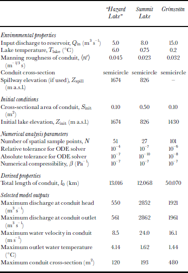
In this section, I apply the modified Spring–Hutter formulation to the problem of simulating outburst floods for the comparatively well-studied cases of “Hazard Lake”, Yukon, Canada, Summit Lake, British Columbia, Canada, and the Grímsvötn reservoir within Vatnajökull ice cap in Iceland. The common physical constants of the models are given in Table 1, and model-specific parameters of the three reference models are listed in Table 2.

The question of whether to adopt the Manning or the Darcy–Weisbach roughness description is not a major issue for most natural flows because the range of discharge for a given river or conduit is unlikely to vary over many orders of magnitude. For outburst floods, however, the decision is important. The relationships between the two descriptions are
and from Equation (23) it is clear that for an assumed constant value of f R the Manning roughness increases as the hydraulic radius increases. Thus the predicted roughness of large conduits is greater than that for small conduits. Hydrologists claim the opposite and would, in fact, assert that even when a constant Manning roughness is assumed (which according to Equation (24) would lead to decreasing Darcy–Weisbach roughness with increasing hydraulic radius) the roughness for large conduits and for high discharge rates is overestimated (e.g. Reference DingmanDingman,1984, p.145). A desirable characteristic of the roughness description is that numerical values of the roughness parameterization do not vary with the scale of the flood. Although neither description satisfies this requirement, the Manning description comes closer to this ideal and is therefore my preferred choice.
“Hazard Lake” flood models
The 1978 flood from glacier-dammed “Hazard Lake” is among the best-studied outbursts and motivated the development of a bottleneck model (Reference ClarkeClarke, 1982) based on a modification of Nye’s theory (Reference NyeNye, 1976). The geometry of the reservoir is very well determined and the geometry of the 13 km flood path through or beneath Steele Glacier is reasonably well constrained. Figure 2a shows the measured hypsometric function (Reference ClarkeClarke, 1982, table 2) for the lake, and Figure 2b summarizes the assumed geometry of the ice surface, bed topography and subglacial flood path (ABC). The elevation of the lake surface and outlet (C) correspond to measured values, as does the distance between the inlet (A) and outlet. The representation of the ice surface for Steele Glacier is taken to be simple but consistent with the 1978 ice topography. There are no measurements of ice thickness, so I have taken the elevation of the seal (B) and the ice thickness above the seal to correspond to those assumed in Reference ClarkeClarke (1982). Lake temperature was not measured in 1978, so water temperature measurements taken in summer 1979 were substituted. The discharge hydrograph for the 1978 flood was calculated by numerical differentiation of the record of lake level vs time and then applying the known hypsometric function of the lake. From the calculated hydrograph, the maximum flood discharge was estimated to be approximately 640 m3 s−1.
Geometry and discharge for “Hazard Lake” outburst floods. (a) Hypsometric function for lake (Reference ClarkeClarke, 1982). (b) Geometry of glacier and subglacial flood routing. (c) Simulated discharge hydrographs. Curve A uses the model and parameters of Reference ClarkeClarke (1982), and the remaining curves are simulated using the present model and data from Tables 1 and 2 (except when otherwise indicated). Curve B is for a circular conduit with Manning roughness of n′ = 0.06 m−1/3 s; curve C is for a semicircular conduit having a perimeter-averaged Manning roughness of 〈n′〉 = 0.045 m−1/3 s and corresponds to the reference model of Table 2; curve D is for a circular conduit and Darcy–Weisbach roughness of fR = 0.20; curve E is for a semicircular conduit and perimeter-averaged Darcy–Weisbach roughness of 〈fR〉 = 0.12.The curves have been time-shifted relative to each other in order to improve their clarity.The slope discontinuity at peak discharge occurs because the flood is terminated by complete drainage of the lake.

Figure 2c shows simulated discharge hydrographs for the 1978 flood. Curve A is the hydrograph calculated in Reference ClarkeClarke (1982) using the bottleneck model and parameters listed in Reference ClarkeClarke (1982, table 3); the Manning roughness for this model is n ′ = 0.105 m−1/3 s and the conduit geometry is circular. The remaining curves were calculated using the Spring–Hutter model as described in the previous section. Curve B is for a circular conduit having a Manning roughness of n ′ = 0.06 m−1/3 s, while curve C corresponds to the “Hazard” reference model of Table 2 and is for a semicircular conduit with a perimeter-averaged Manning roughness of 〈n ′〉 = 0.045 m−1/3 s. (I use angular brackets to draw attention to the fact that the Manning roughness represents a perimeter-averaged value that allows for differing roughnesses of ice and bed. For a circular ice-walled conduit the perimeter-averaged roughness and the conventional Manning roughness n ′ are identical.) Similarly, curves D and E are for a circular conduit with Darcy–Weisbach roughness f R = 0.20 and a semicircular conduit with perimeter-averaged Darcy–Weisbach roughness 〈f R〉 = 0.12, respectively. Despite differences in the modelling assumptions, all the curves are essentially identical. The assumed Manning roughness for the bottleneck model (A) is greater than that for the corresponding Spring–Hutter model (B), and models that assume a semicircular conduit require less flow resistance than those that assume a circular conduit. Although I have expressed a preference for the Manning roughness description, both the Darcy–Weisbach and Manning descriptions are capable of providing visually acceptable hydrographs.
Summit Lake flood model
Figure 3 presents the geometrical assumptions and discharge hydrographs for the model of the 1967 outburst flood from Summit Lake. The hypsometric data (Fig. 3a) are from Reference Clarke and MathewsClarke and Mathews (1981, table 1), and the assumed glacier geometry (Fig. 3b) is consistent with topographic maps and seismic soundings by Reference DoellDoell (1963). Water discharge into the lake was estimated as Q in = 8 m3 s−1 (Reference Clarke and MathewsClarke and Mathews, 1981, p.1456). Lake temperature, measured in 1968, was taken to be 0.75°C (Reference GilbertGilbert, 1969). Discharge hydrographs are presented in Figure 3c. Curve A corresponds to the hydrograph obtained by Reference Clarke and MathewsClarke and Mathews (1981) using a bottleneck model and closely matches the observed hydrograph (see Reference Clarke and MathewsClarke and Mathews, 1981, fig. 3). Curve B presents the results of a Spring–Hutter simulation using the geometric data of Figure 3 and other data from Tables 1 and 2. Although the two curves are virtually identical, the assumed values of Manning roughness differ substantially, being n ′ = 0.12 m−1/3 s for the bottleneck model and 〈n ′〉 = 0.023 m−1/3 s in the present study. Rather than being surprisingly high, as for the bottleneck model, the flow resistance for the Spring–Hutter model is surprisingly low, though not unacceptably low. Instead of assuming a low value for 〈n ′〉 it would be possible to accept a larger value and postulate that the lake temperature exceeded the assumed value of 0.75°C.
Geometry and discharge for Summit Lake outburst floods. (a) Hypsometric function for lake (Reference Clarke and MathewsClarke and Mathews, 1981, table 1). (b) Assumed geometry of glacier and subglacial flood routing. (c) Smooth curve that closely fits the observed discharge hydrograph (A) compared to simulated hydrograph (B). The slope discontinuity at peak discharge occurs because the flood is terminated by complete drainage of the lake.

Grímsvötn flood model
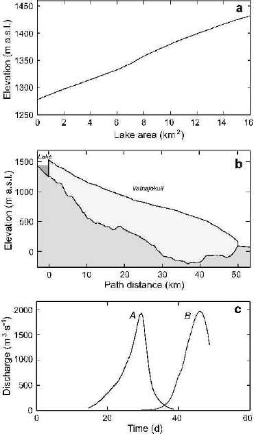
Outburst floods from Grímsvötn have been the most influential in terms of their stimulus to science and prompted the seminal contributions of Reference BjörnssonBjörnsson (1974, Reference Björnsson1988) and Reference NyeNye (1976). I shall take the 1986 outburst flood as the reference flood for Grímsvötn. Though one of the lesser floods, it is well constrained by observations. Figure 4a and b summarize the geometrical data for the lake (Reference BjörnssonBjörnsson, 1992, fig. 2), glacier and subglacial routing (Reference BjörnssonBjörnsson, 2003, fig. 8). Other model input data are given inTables 1 and 2. The lake temperature, taken to be 0.2°C, is based on 1991 measurements (Reference BjörnssonBjörnsson, 1992, p.102), and the water input to the reservoir is Q in = 15 m3 s−1, consistent with estimates by Reference BjörnssonBjörnsson (1988, p.78).
Geometry and discharge for Grímsvötn 1986 outburst flood. (a) Hypsometric function for lake (Reference BjörnssonBjörnsson, 1992, fig. 2). (b) Geometry of glacier and subglacial flood routing (Reference BjörnssonBjörnsson, 1974, fig. 14). (c) Observed (A) and simulated (B) discharge hydrographs.The flood is terminated by complete drainage of the reservoir.
Discharge hydrographs are presented in Figure 4c. Curve A corresponds to the observed hydrograph (Reference BjörnssonBjörnsson,1992, fig. 4) and curve B to the hydrograph simulated using the Spring–Hutter model. A semicircular conduit having a perimeter-averaged Manning roughness of 〈n ′〉 = 0.032 m−1/3 s was assumed. Reference BjörnssonBjörnsson (1992, fig. 9) used a bottleneck model to calculate a similar hydrograph but assumed a roughness of n ′ = 0.08 m−1/3 s.
Results
A common feature of the recalibrated flood models for “Hazard Lake”, Summit Lake and Grímsvötn is that reasonable fits between simulated and observed hydrographs can only be obtained if one assumes that the flow resistance is substantially lower than that used for bottleneck models. In part this can be explained by the assumption of a semicircular rock-floored conduit, but even if a circular ice-walled conduit is assumed it is necessary to accept lower values of flow resistance than for bottleneck models. It can be shown that the significant discrepancy between earlier work and the present study results from shortcomings of the Reference NyeNye (1976) postulate concerning the effectiveness of heat transfer from the conduit to the ice walls (Appendix C). To my knowledge, the Nye postulate has not previously been tested and the apparent failure of this postulate is an important new result. In this section I shall examine additional features of the recalibrated reference models and expose some short-comings of bottleneck models. Note that in all cases t = 0 days signifies the time at which plotting begins. The actual simulations began at substantially earlier times, but the plots focus on the flood itself rather than the slow onset.
Thermal evolution and exit temperature of water
Figure 5 summarizes the spatial and temporal evolution of water temperature for the three reference floods. Temperature curves (labelled lines and left abscissa) are presented for nominal down-flow distances of 0 (the conduit inlet), 0.2l 0, 0.4l 0, 0.6l 0, 0.8l 0 and l 0 (the conduit outlet); discharge hydrographs (dashed curves and right abscissa) are included for reference. Note that the time axis has been arbitrarily shifted so that t = 0 days does not necessarily correspond to the start time for the simulation. Initially the growth of the drainage conduit is extremely slow and, although the magnitude of discharge through the small initial leakage path is small, it is nevertheless sufficient to affect the water temperature in the conduit.
Temporal and spatial evolution of water temperature for outburst flood simulations. Simulated discharge hydrographs (dashed lines) are included for reference. Labelled curves correspond to different down-flow distances relative to the length l0 of the flood path so that 0 corresponds to the conduit inlet and 1 to the outlet. Time zero represents the time at which plotting is initiated but not the actual time at which the simulation was begun. (a) “Hazard Lake” outburst. (b) Summit Lake outburst. (c) Grímsvötn outburst.

Figure 5a shows results for the “Hazard Lake” outburst. Lake temperature was taken to be 6.0°C (Table 2), so the curve for s = 0 does not vary from this value. Near t = 0 days the temperature at s = 0.2l 0 already reflects the influx of warm lake water and has risen from its initial temperature (taken as the pressure-melting temperature of ice) to around 3°C. As the flood progresses, the influence of warm water from the lake is projected farther down the conduit, and at the flood peak the temperature of water exiting the conduit is 4.1°C, indicating that at this stage of the flood the advective transport of heat greatly exceeds the loss by melting of the conduit walls.
In contrast, the Summit Lake outburst simulation (Fig. 5b) illustrates the effects of a comparatively cold water reservoir. The lake temperature is 0.75°C as indicated by the curve for s = 0. At t = 0 days the water temperature at s = 0.2 l 0 is substantially colder than the lake but nonetheless above the melting temperature of ice. Farther down-flow the temperatures are below 0°C but above or near the pressure-melting temperature at these locations. As the flood progresses, the temperature along the conduit increases until at around 2.5 days the water temperature in the conduit everywhere exceeds the lake temperature. This additional warming is caused by viscous dissipation in the conduit. At this stage of the flood, the water temperature increases with down-flow distance, the exact opposite of the situation for the “Hazard Lake” flood. The maximum water temperature during the flood occurs at the conduit exit and equals 1.6°C, substantially above the lake temperature.
The Grímsvötn outburst simulation (Fig. 5c) has clear similarities with that for Summit Lake, although the temperature curves have more character. Again the lake temperature is only slightly above the melting temperature, and viscous dissipation is important in enabling the flood to develop. By t = 6 days the water temperature in the drainage conduit is everywhere above the lake temperature even though the flood is only beginning to enter its rapid growth phase. As with the simulated outburst for Summit Lake, maximum water temperature occurs at the conduit outlet. The predicted maximum water temperature is 1.4°C, in contrast to the assumed lake temperature of 0.2°C. In fact such a high outlet temperature has not been observed and this suggests some shortcomings that I shall discuss subsequently.
Evolution of fluid potential gradient and effective pressure
The Spring–Hutter model permits detailed examination of the evolution of water pressure and potential energy gradient as an outburst flood progresses. Of special interest is the spatial position of flow constrictions in the drainage conduit and whether these constrictions remain fixed in space or migrate as the flood progresses. A fundamental assumption ofthe Nye model is that the fluid potential gradient ∂ϕ/∂s is reasonably well approximated by its length-averaged value 〈∂ϕ/∂s〉, whereas a fundamental assumption of bottleneck models is that the seal is the dominant flow constriction at all stages of an outburst flood. These assumptions cannot be tested without resorting to a more comprehensive model such as that of Spring and Hutter. To test the Nye assumption and to identify regions of flow constriction, I evaluate the spatial gradient of the hydraulic potential ϕ = p w + ρ w gZ k and seek regions where −∂ϕ/∂s is greatest or, equivalently, where ∂ϕ/∂s is least. Letting s * denote the instantaneous value of s at which −∂ϕ/∂s is maximum, one can plot s *(t); and this locates the down-flow position of the bottleneck as the flood progresses. A more detailed picture of flow constrictions is obtained by plotting ∂ϕ(s, t)/∂s over the course of the flood. For the Nye assumption to be valid, the potential energy gradient should vary with time but not with distance along the conduit. A second matter of interest is the effective pressure p e = p i − p w, which is diagnostic of whether water pressure exceeds the ice flotation pressure. As shall be shown, the water pressure in the conduit can greatly exceed the ice overburden pressure, and this has implications for the dispersal of water along the ice–bed interface, hydraulic fracturing of the ice walls and the escape of water by artesian outflow to the glacier surface.
“Hazard Lake” model results
Figure 6 shows the temporal evolution of fluid potential gradient and effective pressure for the “Hazard Lake” reference model. The spatial location of the dominant flow constriction (dashed line and right abscissa) and the flood hydrograph (solid line and left abscissa) are plotted in Figure 6a. Interestingly, the flow constriction is located at the glacier terminus (s * = 13 km) throughout the observation interval, and at no time is the flow constriction located at the “seal” defined by the maximum ice thickness (s seal = 1 km in Fig. 2b). Apparentlythe sensible heatof lake water is sufficient to overcome flow constrictions near the inlet and it is the lower temperature of water near the glacier terminus that maintains a constriction at the outlet. Although the seal may have played a role in controlling the onset of the flood, it does not serve as the controlling flow constriction once the flood has started to develop.
Temporal and spatial evolution of effective pressure and flow constriction for “Hazard Lake”outburst simulation. (a) Simulated discharge hydrograph (solid line and left abscissa) and down-flow distance of the flow “bottleneck”as a function of time (dashed line and right abscissa). (b) Spatio-temporal evolution of fluid potential gradient ∂φ(s, t) = ∂s. Contours are not labelled, but dark shading corresponds to regions where potential energy dissipation is concentrated, hence regions where flow is restricted. (c) Spatio-temporal evolution of effective pressure pe(s, t) in conduit. Negative values of effective pressure correspond to water pressures exceeding the ice flotation pressure. (Contours are in units of MPa.)

Figure 6b shows the pattern of fluid potential gradient associated with the “Hazard Lake” outburst simulation. The contours have not been labelled because it is the pattern, rather than the actual magnitudes, that commands interest. Dark shading corresponds to regions where potential energy dissipation is concentrated, and it is clear that this is greatest in the lower reaches of the drainage conduit and decreases monotonically toward the lake. The fact that the fluid potential gradient varies spatially as well as temporally indicates that the Nye assumption is not satisfied. The putative “seal” at s seal = 1 km seems irrelevant to this pattern.
The simulated distribution of effective pressure during the “Hazard Lake” outburst is given in Figure 6c with contours labelled in MPa. The 0 MPa contour separates the region of ice flotation (negative effective pressure) from that where ice pressure exceeds water pressure. Note that water pressure exceeds the ice flotation pressure over virtually the entire length of the conduit for the entire observation interval and that, over the middle section of the conduit, water pressure exceeds ice overburden pressure by at least 1 MPa for the first 2.3 days of the observation window. When reckoned in terms of the equivalent water level, this corresponds to a water column >100 m above the flotation level and would be sufficient to drive water to the surface of Steele Glacier if cracks or other water paths existed.
Summit Lake model results
A similar analysis of the Summit Lake outburst simulation produces a more interesting story (Fig. 7). Figure 7a shows the position of the dominant flow constriction as a function of time (dashed line and right abscissa) with the flood hydrograph included for reference (solid line and left abscissa). During the early development of the flood the flow constriction is located at the glacier terminus (s * = 12 km in Fig. 3b), but at around t = 2.5 days the constriction migrates up-glacier, first in a regular fashion but then in a discontinuous jump from s* ≈ 8 km to the conduit inlet at s * = 0 km. The up-flow migration of the flow constriction appears to be associated with the evolving thermal conditions in the drainage conduit (Fig. 5b). At around t = 2.5 days the water temperature at the conduit exit begins to exceed the lake temperature so that concentrated viscous dissipation near the conduit exit is no longer required to overcome creep closure by ice pressure.
Same as Figure 6, but for Summit Lake outburst simulation.

Figure 7b shows the pattern of the fluid potential gradient and clarifies the nature of the previously noted jump in s *. Dark shading indicates regions where potential energy dissipation is concentrated, and the overplotted dashed line indicates the migration of the flow constriction, as also plotted in Figure 7a. Note that during the early stages of the flood, potential energy dissipation is concentrated in the lower reaches of the conduit, and during the rapid growth phase of the flood the potential energy dissipation is concentrated near the conduit inlet. The jump in s * is clearly related to the morphology of the surface ∂φ(s, t)/∂s. As for the “Hazard Lake” simulation, the Nye assumption clearly fails.
Figure 7c shows the distribution of effective pressure in the conduit as the flood progresses. The contours are labelled in MPa and the zero contour is clearly indicated. Water pressure exceeds the ice flotation pressure only in the earliest stages of the flood, and the overpressure never exceeds 0.6 MPa.
Grímsvötn model results
For the Grímsvötn flood simulation the flow constriction shows behaviour similar to that found in the Summit Lake simulation. In the early stages of the flood, the flow constriction is located near, though not at, the conduit outlet (s * ≈ 44 km), but, as the flood begins to accelerate, the flow constriction first jumps to the conduit outlet and then at around 5.5 days jumps up-flow to the conduit inlet where it remains until the flood terminates (Fig. 8a). An examination of the contour diagram for ∂φ(s, t)/∂s (Fig. 8b) indicates that the spatial pattern of the fluid potential gradient is complex, presumably because of the complex bed topography assumed for this model (Fig. 4b), and it is evident that the Nye assumption is not satisfied. The effective pressure distribution (Fig. 8c) is also complicated for this model. Superflotation pressures only obtain during the early development of the flood and cease to exist after t = 6.5 days.
Same as Figure 6, but for Grímsvötn outburst simulation.

Influence of “seal” position on peak discharge
If it could be demonstrated that bottleneck simulations and Spring–Hutter simulations yielded essentially similar results, even if they required different calibrations for flow resistance, one could dispense with the unnecessary complication of the Spring–Hutter model. The following numerical experiments demonstrate that this is not the case. Bottleneck models reduce the geometric description of the flood path to the following essentials: input elevation Z k (0), output elevation Z k(l 0), seal elevation Z k(s seal) and ice surface elevation at the seal Z i(s seal). There is a further implicit assumption that the seal is near the lake so that s seal → 0. Figure 9 shows five different glacier geometries that have identical values of Z k(0), Z k (l 0), Z k(s seal) and Z i(s seal) and differ only in the value of s seal which varies from 1 km (ice geometry A) to 12 km (ice geometry E) for a 20 km long drainage conduit. For each geometry Z k(0) = 500 m a.s.l., Z k(l0) = 0 m a.s.l., Z k(s seal) = 0 m a.s.l. and Z i(s seal) = 800 m a.s.l. The conduit is assumed to be semicircular with a perimeter-averaged Manning roughness of 〈n ′〉 = 0.04 m−1/3 s for all runs. Figure 10 presents a suite of simulated flood hydrographs corresponding to each of the assumed glacier geometries and lake temperatures of 0.5°C (Fig. 10a), 2.0°C (Fig. 10b) and 6.0°C (Fig. 10c). For every case there is a systematic decrease in peak discharge magnitude as the distance between the lake and seal is increased. The effect is most pronounced when the lake temperature is low (Fig. 10a), and least pronounced when it is high (Fig. 10c). Examining Figure 10c, one could argue that the influence of seal location is not sufficiently pronounced to justify the added complexity of Spring–Hutter models, but this is clearly not the case for Figure 10a. Thus, in general, it appears that it is necessary to employ Spring–Hutter modelling before one can decide whether bottleneck models are an acceptable simplification.
Five simple glacier geometries having identical values for inlet and outlet elevation and ice thickness at the “seal”. For geometry A the location of maximum surface elevation and minimum bed elevation are each labelled A, and similarly for the remaining four geometries. For geometry A the seal is closest to the lake, and for geometry E it is farthest down-flow.

Effect of water temperature and routing geometry on simulated discharge hydrographs. A–E refer to the subglacial routings associated with glacier illustrated in Figure 9. (a) Lake temperature 0.5°C. (b) Lake temperature 2.0°C. (c) Lake temperature 6.0°C.

Discussion and Conclusions
Much attention could be devoted to the issue of calibrating the flood models, i.e. finding proper assignments of loosely constrained parameters such as the hydraulic roughness of the conduit. In the present work, I have only attempted to seek rough calibrations because the available data do not justify a more ambitious attack. For example, lake temperature data and outburst flood data are rarely collected simultaneously and thus there is an ambiguous association between the assumed value for T lake and a given outburst flood. Errors in T lake affect the predicted flood magnitude and thus can give rise to false calibrations of hydraulic roughness. As already mentioned, the temperature of “Hazard Lake” was taken in 1979, whereas the flood was measured in 1978; that for Summit Lake was measured in 1968 but the flood was monitored in 1969; for Grímsvötn the measurements were taken in 1991 and are applied to the 1986 flood. Present models also assume an isothermal lake, whereas reported measurements (e.g. Reference GilbertGilbert, 1969; Reference BjörnssonBjörnsson, 1992) indicate that the lakes, unsurprisingly, have a thermal structure which could affect the detailed form of the outburst hydrograph. One hopes that the ongoing study of outburst floods from Hidden Creek Lake, Alaska, U.S.A. (Anderson and others, in press), will yield the comprehensive data that will allow these outstanding problems to be addressed.
The predicted temperature of water exiting the conduit at the flood climax (Fig. 5) is substantially higher than the temperature suggested by observations. For example, Reference RistRist (1955) reported a water exit temperature of 0.05°C for the 1954 outburst from Grímsvötn, whereas the reference model for the 1986 outburst (Table 2) predicts a temperature of 1.44°C. Reference BjörnssonBjörnsson (1992, p.104) has considered this problem of the models and states:
The actual heat transfer by flowing water during jökulhlaups is more effective than accounted for by Reference Spring and HutterSpring and Hutter’s (1981) model for simulation of drainage (as pointed out by Reference NyeNye (1976)). The empirical heat transfer equation may be wrong at the high Reynolds numbers in the jökulhlaups. On the other hand, melting of ice may not be restricted to the walls, because ice needles, eroded by debris and sand from the walls, mix with the water.
I have explored the consequences of replacing Equation (19) (Reference McAdamsMcAdams, 1954) by alternative expressions (Reference Bird, Stewart and LightfootBird and others, 1960) and found little to distinguish them. If the problem is associated with the heat-transfer empiricism, then existing formulas are either inappropriately used or badly wrong. One possible source of difficulty (personal communication from N. F. Humphrey, 1991) is that conventional heat-transfer formulas, which assume warm water entering a pipe, may not apply to the situation of a fluid heated by viscous dissipation in its frictional boundary layer. This concern warrants further study. Björnsson’s second explanation, that outburst flood waters are a dilute suspension of ice crystals, also strikes me as plausible. This possibility should be vigorously explored, from both an observational and theoretical perspective. It would not be challenging to extend the Spring–Hutter work by adding a balance equation for suspended ice crystals that would include an ice production term associated with mechanical abrasion of the ice walls and a mass-loss term associated with melting of the crystals.
The predicted jumps in bottleneck position (Figs 7 and 8) and the associated rapid rearrangements of conduit pressure are extremely interesting. It is possible that such rapid structural adjustments can produce unexpected features in discharge hydrographs that have been previously attributed to additional phenomena such as tunnel collapse.
Superflotation water pressures are predicted for all three reference models. Excess water pressure would be expected to drive water out of the conduit and along the ice–bed interface, creating the possibility of tapping into pre-existing subglacial drainage paths. An observable consequence of such behaviour would be the formation of more than one drainage outlet for a single flood. Reference BjörnssonBjörnsson (1998) notes that for large outbursts from Grímsvötn as many as 10–15 highcapacity drainage tunnels can develop. From this perspective, it is interesting that for all three models the water pressure is highest during the flood onset and decreases as the flood peak is reached. High-capacity outlets can only exist if they are formed early. If water pressure greatly exceeds the ice pressure then an englacial crack system can develop by hydrofracturing. If water pressure (expressed as hydraulic head) exceeds the ice thickness, water can be routed from the drainage conduit to the glacier surface following a system of existing or newly created cracks, as observed for Grímsvötn floods (Reference BjörnssonBjörnsson, 1998). Evidence for both ice fracturing and supraglacial water routing is especially well documented for the huge outburst of November 1996 (Reference Roberts, Russell, Tweed and KnudsenRoberts and others, 2000;Reference Waller, Russell, van Dijk and KnudsenWaller and others, 2001; Björnsson, 2002; Reference JóhannessonJóhannesson, 2002).
The main conclusions of this study are the following:
-
1. With a minor adjustment of the governing equations, the Spring–Hutter formulation can be rendered into a system of equations that is straightforward to solve using the numerical method of lines. Recast in this manner, it provides a powerful tool for detailed examination of the hydraulics and thermodynamics of outburst floods.
-
2. A recalibration of the Manning roughness for outburst floods using the Spring–Hutter model indicates that previous estimates of flow resistance are unreasonably high. The cause of this discrepancy can be traced to the Reference NyeNye (1976) postulate that dT w/dt = 0 along the drainage conduit. All previous work using bottleneck models is based on this assumption and thus seriously flawed. The new estimates of channel roughness, though provisional, are consistent with the Manning roughness of natural streams and rivers. Additional work remains to be done in improving the calibration of these models, but better observational data are required before substantial progress can be made.
-
3. Careful observations of outlet temperature, preferably as a function of time, are lacking, but the Spring–Hutter model, together with earlier work, appears to overestimate the temperature of water exiting the subglacial drainage conduit. It is possible that empirical formulas for heat exchange at the conduit walls are incorrect or inappropriate, but the importance of mechanical abrasion as a process for enlarging ice-walled conduits needs investigation. Even a small amount of abrasion could have a substantial influence on water temperature.
-
4. The Spring–Hutter model predicts that superflotation water pressures can develop in the drainage conduit, in qualitative agreement with field observations. Excess pressure is greatest at early stages of the outburst and decreases as the flood progresses.
-
5. The fluid potential gradient along the conduit is not well represented by its value averaged over the length of the conduit.
-
6. Bottleneck models are unable to capture many important features of outburst flooding, and the basic assumption of bottleneck models, that a spatially fixed flow-controlling seal exists close to the water reservoir, is not generally satisfied. Flow constrictions appear to be highly mobile during the course of an outburst flood, and for some floods the dominant flow constriction is located near the tunnel outlet for much of the flood duration.
What is the prospect for using simulation models to predict glacier flood hazards? It is doubtful that the simple bottleneck models can be reinstated, but this is not necessarily a discouraging outcome. The main justification for bottleneck models was that they were simple to implement, whereas Spring–Hutter models, primarily because of computational challenges, were not. This is no longer the case. Furthermore, Spring–Hutter models have a superior physical basis and, although they seem to require more detailed information about the glacier surface and bed topography, they can perform adequately when such information is sketchy.
Acknowledgements
This paper is a contribution to the Climate System History and Dynamics program that is jointly sponsored by the Natural Sciences and Engineering Research Council of Canada (NSERC) and the Meteorological Service of Canada. I am extremely grateful to the Killam Canada Council Fellowship Program and the University of British Columbia for financial support during a research leave at the Scott Polar Research Institute, Cambridge, U.K., and to the Director and staff of the Institute for their hospitality. H. Björnsson gave me a much treasured copy of his monumental dr. philos. thesis monograph on the Hydrology of ice caps in volcanic regions. Belatedly (by more than two decades), I would like to thank U. Spring and K. Hutter for their pathbreaking work on this subject. Their monumental paper in the International Journal of Engineering Science is in a class of its own and has been unjustly neglected. Finally, I thank S. P. Anderson, F. S. L. Ng, C. F. Raymond and Scientific Editor J. S. Walder for helpful criticisms.
Appendix A
Numerical Stiffness
Waves of compression in rigid tubes
The problem of numerical stiffness arises because the system of conservation equations upon which the Spring–Hutter formulation is based admits wave-like solutions as well as the desired solution for water flow. Such waves might be associated with a distensible conduit containing an incompressible fluid or a rigid-walled conduit containing a compressible fluid. In the former case, the speed of pressure waves is ![]() , where ρ is the fluid density and γ is a coefficient of distensibility (the fractional change in conduit cross-sectional area with pressure); in the latter case, the wave speed is
, where ρ is the fluid density and γ is a coefficient of distensibility (the fractional change in conduit cross-sectional area with pressure); in the latter case, the wave speed is ![]() , where β is the coefficient of compressibility (the fractional change in fluid density with pressure). The case of a distensible conduit containing a compressible fluid is also physically realistic but adds nothing worthwhile to our analysis. Note that for an incompressible fluid in a non-distensible conduit β = 0 and γ = 0 and the speed both of waves of distension and of waves of compression becomes infinite. The challenge of resolving fast-travelling waves while simultaneously calculating the much slower motion of the fluid itself underlies the numerical stiffness of the Spring–Hutter equations. To avoid these difficulties it is necessary to introduce a degree of fluid compressibility or conduit distensibility so that the associated pressure waves are slowed. I have explored both approaches to suppressing stiffness and believe that introducing fluid compressibility yields the strategy that is the more straightforward conceptually and computationally.
, where β is the coefficient of compressibility (the fractional change in fluid density with pressure). The case of a distensible conduit containing a compressible fluid is also physically realistic but adds nothing worthwhile to our analysis. Note that for an incompressible fluid in a non-distensible conduit β = 0 and γ = 0 and the speed both of waves of distension and of waves of compression becomes infinite. The challenge of resolving fast-travelling waves while simultaneously calculating the much slower motion of the fluid itself underlies the numerical stiffness of the Spring–Hutter equations. To avoid these difficulties it is necessary to introduce a degree of fluid compressibility or conduit distensibility so that the associated pressure waves are slowed. I have explored both approaches to suppressing stiffness and believe that introducing fluid compressibility yields the strategy that is the more straightforward conceptually and computationally.
First I shall demonstrate the existence of a wave of compression in the fluid. The melting terms will be dropped for this preliminary analysis. Consider a slow-flowing or static compressible fluid of density ρ w in a rigid walled conduit. The tube is oriented so that the distance coordinate s is alignedwiththe axis of the tube and the tube will be viewed as essentially straight. From conservation of mass
and the momentum-balance equation (neglecting wall friction) is
With specific reference to water-filled conduits, I adopt the following definitions:
Assuming that the advection terms v∂ρ w/∂s and v∂v/∂s can be neglected and that the pressure effect on density is small, Equations (A1) and (A2) can be approximated as
Taking the t derivative of Equation (A8) and the s derivative of Equation (A9) and eliminating ∂2 v/∂s∂t gives
which has the form of a wave equation for a pressure disturbance propagating at speed ![]() . A similar analysis (e.g. Reference LighthillLighthill, 1978, p. 92–94; Reference PedleyPedley, 1980, p.73) can be applied to demonstrate the existence of waves of distension in elastic tubes containing incompressible fluids.
. A similar analysis (e.g. Reference LighthillLighthill, 1978, p. 92–94; Reference PedleyPedley, 1980, p.73) can be applied to demonstrate the existence of waves of distension in elastic tubes containing incompressible fluids.
Strategy 1: compressible fluid
Turning to the Spring–Hutter equations, I introduce a slight fluid compressibility so that the mass-balance equation is written
which, assuming that v∂ρ w/∂s ≪ ∂ρ w/∂t, I approximate as
and using Equation (A7) write
The slight effect of compressibility on the momentum- and energy-balance equations is neglected so that the complete system of equations is


Strategy 2: distensible conduit
An alternative strategy for reducing numerical stiffness is to assume that water is incompressible but the conduit is distensible so that Equation (A15) becomes
where the final term expresses the effect of distensibility and follows from the definition (A6) and
where ∂S ′/∂t is the rate of change of cross-sectional area that results from conduit distension. Rearranging Equation (A18) and making appropriate changes to the continuity equation gives
to replace Equations (A14) and (A15). As previously, the momentum- and energy-balance expressions are unaffected.
I have explored the merits of the alternative strategies for reducing numerical stiffness and conclude that strategy 1 is the superior one because it yields accurate solutions with integration times that are substantially less than those for strategy 2.
Appendix B
Generalization to Non-Circular Conduits
Flow resistance of semicircular conduits
Semicircular conduits are assumed to be ice-roofed and bed-floored. The Darcy–Weisbach roughness of ice will be denoted fi and that for bed material fb. Turbulent discharge in a conduit is driven by a potential energy gradient acting over the conduit cross-section so that S(−∂φ/∂s) is the force per unit length of conduit that drives fluid motion.This force is resisted by the wall stress τ 0 acting over the wetted perimeter of the conduit P w, so that force balance requires
For turbulent flow in a conduit having a single roughness value of f R the wall stress is given by the standard relation
For conduits having a mixed perimeter of ice and bed material, the wall stress acting on the ice roof can differ from that acting on the bed floor so that locally
and
where P i is the ice contact perimeter, P b is the bed contact perimeter, P w = P i + P b and τ 0 can be regarded as the perimeter-averaged wall stress. From Equations (B2–B5) it follows that for mixed-perimeter conduits
where
For a semicircular bed-floored conduit, P i = πR, P b = 2R, P w = (π + 2)R and
Using the Manning roughness description, an expression equivalent to Equation (B7) is obtained by applying the conversion formula
to Equation (B7) to obtain

which for a semicircular bed-floored conduit gives

Generalization of mass- and heat-transfer relations
To generalize from circular conduits to non-circular ones, I follow the standard approach of replacing D (the diameter of a circular conduit) with D = 4R H, where the hydraulic radius is taken as R H = S/P w where P w is the conduit perimeter. (Because I assume that the conduit is completely water-saturated, the distinction between the perimeter and the wetted perimeter is unnecessary.) For a circular cross-section R H = D = 4, as required, and for a semicircular cross-section R H = πD = 4(π + 2). In terms of the hydraulic radius, the Reynolds number is written
The heat flux from the conduit to its walls is governed by an expression of the form q = hΔT, where h is an empirical heat-transfer coefficient and ΔT is the temperature difference between the fluid and the conduit walls. The expression h = 0.023 Pr2/5 Re4/5 K w /D, extracted from Reference McAdamsMcAdams (1954), has been the most widely adopted for glaciological calculations; similar empiricisms can be found in Reference Bird, Stewart and LightfootBird and others (1960). Following the prescription D = 4R H and accepting the McAdams equation for h gives
The mass rate of melting per unit area of conduit surface is simply ![]() , where L is the latent heat of melting and the mass rate of melting per unit length of conduit is
, where L is the latent heat of melting and the mass rate of melting per unit length of conduit is ![]() whereP
m isthe melting perimeterofthe conduit. For a circular ice-walled conduit P
m = πD, but for a semicircular rock-floored conduit P
m = 1/2πD. To summarize,
whereP
m isthe melting perimeterofthe conduit. For a circular ice-walled conduit P
m = πD, but for a semicircular rock-floored conduit P
m = 1/2πD. To summarize,
Appendix C
Examination of Nye Heat-Transfer Assumption
The heat-transfer analysis of Reference NyeNye (1976) is based on the postulate that the material derivative of water temperature dT
w/dt = ∂T
w/∂t + v∂T
w/∂s vanishes along the flow path. Applying this condition to Equation (10) and making the approximation that ![]() gives
gives
for the melting rate. Reference ClarkeClarke (1982) accepted this assumption and added the effect of lake temperature to obtain an expression equivalent to
where Nu = 0.023 Pr2/5 Re4/5 if the Reference McAdamsMcAdams (1954) formula is accepted. The implication of both Equations (C1) and (C2) is that frictional energy release is directly converted to melting of the ice walls, whereas in the Spring–Hutter formulation

implying that released frictional energy leads to an increase in water temperature which in turn leads to melting. Because it is not possible to examine the effects of the Nye assumption without stepping beyond the limitations of the Nye theory, the assumption has never been closely scrutinized. To do so I must distort the physics of the Spring–Hutter formulation by treating frictional energy and sensible heat as having separable effects. Frictionally generated energy is converted to melt, whereas sensible heat of water is transferred to the conduit walls at a rate predicted by the empirical heat-transfer formula. Thus Equations (C3) and (C4) are modified to give

Substituting the above for Equations (10) and (20) in the Spring–Hutter formulation and repeating the simulations for “Hazard Lake”, Summit Lake and the 1986 Grímsvötn flood, I find that simulations performed using bottleneck models (which of necessity employ the Nye heat-transfer assumption) and Spring–Hutter simulations are in good agreement and that the predicted flood magnitude is much larger than predictions based on the correctly implemented Spring–Hutter equations. In order to force the observed and predicted peak discharges to agree, it is necessary to increase the roughness of the conduit. Because the Nye postulate overestimates the rate of heat transfer to the ice walls, it also overestimates the cross-sectional area of the conduit which in turn yields an excessively high discharge rate. The very high values of Manning roughness inferred by Reference NyeNye (1976) and confirmed by subsequent studies using bottleneck models (e.g. Reference ClarkeClarke, 1982; Reference BjörnssonBjörnsson, 1992) result from shortcomings of the Nye heat-transfer postulate.


