


1. Introduction
The Greenland Ice Sheet (GrIS) lost mass at a rate of 286 ± 20 Gt a−1 in 2010–2018, of which 44% was due to discharge from tidewater glaciers (Mouginot and others, Reference Mouginot2019). Such glaciers drain 88% of the GrIS (Rignot and Mouginot, Reference Rignot and Mouginot2012), making their dynamical behaviour an important target of study when assessing the current and future state of the GrIS. With annual contributions approaching 1 mm a−1 to sea-level rise (IPCC, 2019), the GrIS has changed significantly from a stable mass-balance state 40 years ago (Mouginot and others, Reference Mouginot2019). Hence, predicting the future behaviour of the GrIS and the ensuing change in sea level is only becoming more urgent.
However, Greenlandic tidewater glaciers present a challenging environment, leaving many important processes poorly understood. The thickness (typically several hundreds of metres or more) and speed (often several kilometres a year) of these glaciers make access to the basal environment very difficult. Only a couple of studies have reported direct borehole observations of the base from such glaciers (Lüthi and others, Reference Lüthi, Funk, Iken, Gogineni and Truffer2002; Doyle and others, Reference Doyle2018) and studies of their subglacial hydrology (e.g. Sole and others, Reference Sole2011; Schild and others, Reference Schild, Hawley and Morriss2016; Vallot and others, Reference Vallot2017) and basal conditions (e.g. Hofstede and others, Reference Hofstede2018; Booth and others, Reference Booth2020) are far fewer in number than on land-terminating portions of the ice sheet (e.g. Sole and others, Reference Sole2013; Tedstone and others, Reference Tedstone2013, Reference Tedstone2015; Davison and others, Reference Davison, Sole, Livingstone, Cowton and Nienow2019; Williams and others, Reference Williams, Gourmelen and Nienow2020). This means characterisation of the physical basal properties and subglacial hydrology of Greenlandic tidewater glaciers is very limited. At the same time, observations of behaviour and morphology at the calving front are also limited, both in Greenland and globally, due to the dangerous and inaccessible nature of this environment, meaning calving and submarine-melt processes are also poorly constrained by the available data. Recent work has started to improve this paucity (e.g. Jackson and others, Reference Jackson2017, Reference Jackson2019; Cassotto and others, Reference Cassotto2018; Sutherland and others, Reference Sutherland2019; Vallot and others, Reference Vallot2019; Xie and others, Reference Xie, Dixon, Holland, Voytenko and Vaňková2019), particularly with regards to observations of meltwater plumes at the calving front (e.g. Jackson and others, Reference Jackson2017, Reference Jackson2019; Jouvet and others, Reference Jouvet2018; Slater and others, Reference Slater2018; Hewitt, Reference Hewitt2020), but, overall, many aspects of tidewater glaciers remain under-observed and poorly characterised.
Computer modelling provides an avenue for ameliorating this lack of direct observations and for predicting the future behaviour of Greenland's tidewater glaciers, but the complexity of these systems has made it difficult to implement realistic fully coupled models. Simulating calving is particularly challenging, as the development of a simple calving law, if one is achievable, remains elusive (Benn and others, Reference Benn, Cowton, Todd and Luckman2017; Benn and Åström, Reference Benn and Åström2018), requiring the use of computationally expensive 3D models to reproduce calving with a degree of realism without calibration or tuning (Todd and others, Reference Todd2018, Reference Todd, Christoffersen, Zwinger, Råback and Benn2019). Introducing and coupling subglacial hydrology and meltwater plumes, perhaps the two most important additional and under-observed sets of processes, to such models adds a further layer of computational complexity, meaning that attempts to simulate the full tidewater-glacier system have hitherto only studied selected processes in an uncoupled manner in order to keep the computation time within reasonable limits (Vallot and others, Reference Vallot2018). Such models are also difficult to validate, owing to the number and variety of input datasets meaning that finding a fully independent validation dataset is not necessarily straightforward.
This study presents fully coupled simulations of ice flow, calving, subglacial hydrology and convective meltwater plumes within the 3D, full-Stokes Elmer/Ice modelling suite, with application to Sermeq Kujalleq (Store Glacier; henceforth referred to simply as Store) in west Greenland. With a two-way coupling between ice velocity and basal effective pressure, as well as the impact of meltwater plumes on terminus dynamics, the coupled models capture the primary glaciological processes that control tidewater glacier behaviour, revealing the complex coupled nature of the glacier's interaction with evolving hydrological systems as well as with the ocean.
2. Data and methods
The study site (Section 2.1), model set-up (Section 2.2) and overall modelling procedure (Section 2.3) are described below. Details are included on how the individual model components are coupled within the overall framework of Elmer/Ice (Gagliardini and others, Reference Gagliardini2013) and how the model was spun up.
2.1. Study site
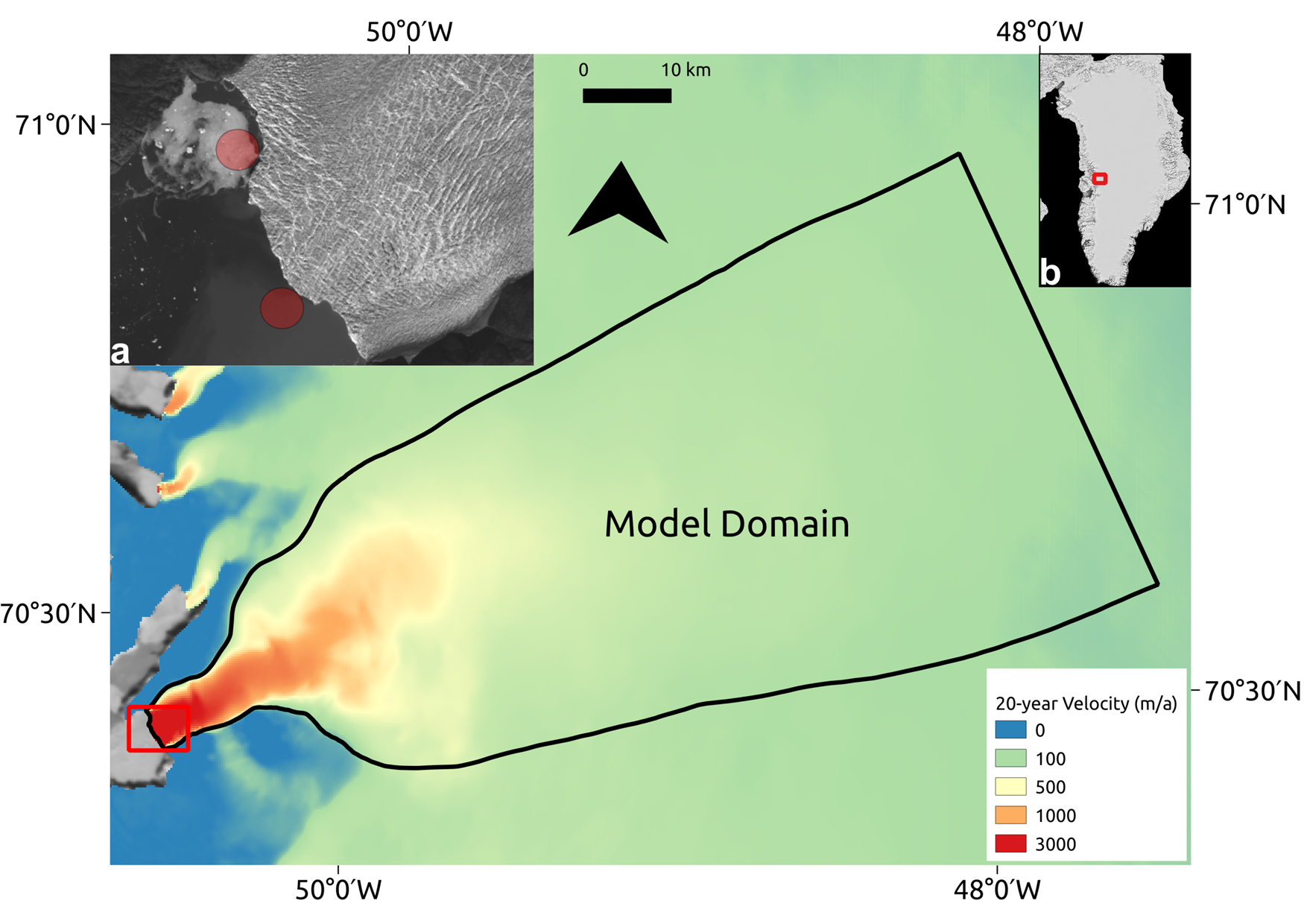
Sermeq Kujalleq (or Store), which is one of the largest tidewater outlet glaciers on the west coast of Greenland (70.4°N, 50.55°W), flows into Ikerasak Fjord (Ikerasaup Sullua) at the southern end of the Uummannaq Fjord system (Fig. 1). The calving front is 5 km wide, with surface velocities of ~6 km a−1 (Joughin and others, Reference Joughin, Smith and Howat2018). The terminus is pinned between narrow fjord walls and a sill on the sea floor, making the terminus position relatively stable despite the trunk of the glacier flowing through a deep trough extending to nearly 1000 m below sea level (Rignot and others, Reference Rignot, Fenty, Xu, Cai and Kemp2015). With no observed retreat since 1985 (Catania and others, Reference Catania2018), the glacier represents a stable Greenland outlet glacier and is an ideal target for modelling studies aiming to understand the ‘natural’ state of a tidewater glacier. Store could, however, retreat rapidly, should increasing melt force the terminus backwards from its current pinning point (Catania and others, Reference Catania2018).
Model domain of Store (main image). Background shows the 20-year velocity average (1995–2015) from the MEaSUREs dataset (Joughin and others Reference Joughin, Smith, Howat and Scambos2016; Joughin and others, Reference Joughin, Smith and Howat2018). Inset (a) shows a zoomed-in view of the terminus (red rectangle in main image). Red circles show approximate areas of observed surfacing plumes. Background shows Landsat view of Store (from 22/07/2016). Inset (b) shows Store's location (red rectangle) in Greenland. Background image from MODIS.
2.2. Model set-up
In this study, we use the open-source, 3D, full-Stokes Elmer/Ice modelling suite (Gagliardini and others, Reference Gagliardini2013), which includes the GlaDS hydrological model (Werder and others, Reference Werder, Hewitt, Schoof and Flowers2013). The work builds on Cook and others (Reference Cook, Christoffersen, Todd, Slater and Chauché2020) who used GlaDS and a 1D plume model to investigate subglacial hydrology and plume-induced frontal melting at Store, with only unidirectional coupling with the overlying ice (so hydrology affects dynamics, but not vice versa). We build on that study by the addition of the calving model detailed in Todd and others (Reference Todd2018) and the implementation of two-way coupling between the overlying ice and the subglacial hydrology. Hence, our model effectively couples ice flow not only with evolving hydrological drainage systems, but also with convective plumes driven by the subglacial fresh water discharge, which leads to undercutting of the terminus and calving. As such, our coupled models provide unique insight to the coupling between all the interacting components of a tidewater glacier system and an evolving glacier geometry. We model the years 2012 and 2017 as in our previous work on this subject (Cook and others, Reference Cook, Christoffersen, Todd, Slater and Chauché2020).
2.2.1. Ice flow and calving model
This study uses the calving implementation of Elmer/Ice as described by Todd and others (Reference Todd2018, Reference Todd, Christoffersen, Zwinger, Råback and Benn2019). The model domain captures the catchment of Store, with the upstream limit defined as the 100 m a−1 velocity contour (110 km inland) and a boundary condition specifying the observed velocity there as imposed inflow. A no-slip condition is imposed on the lateral boundaries, which capture the two sides of the catchment. To allow a better and more realistic representation of glacier flow near the terminus, we apply a Glen enhancement factor of 6.0 along observed shear margins on the lower trunk where ice flows into the sea (Chudley and others, Reference Chudley2021). This equates to a doubling of ice deformability (Placidi and others, Reference Placidi, Greve, Seddik and Faria2010), which, lacking data, is a reasonable assumption given the observed high strain rates. We also impose a sea-water pressure condition on the calving front and its base.
The glacier terminus is allowed to float where the ice thickness is small enough to permit it, which makes the simulation of the grounding line more realistic than in our previous study (Cook and others, Reference Cook, Christoffersen, Todd, Slater and Chauché2020). The addition of this process also means that three free surfaces are present and allowed to evolve throughout each simulation. The upper free surface is subject to a surface mass-balance accumulation flux (which may be negative, representing ablation) boundary condition, varying daily to provide realistic mass forcing for the model. This is taken from RACMO 2.3p2 data provided daily with a 1 km spatial resolution (van Wessem and others, Reference van Wessem2018). The bottom free surface consists of any parts of the glacier terminus that have become ungrounded, and to which a seasonally varying basal melt rate of 2.3 m d−1 in winter and 4.2 m d−1 in summer is applied, following Todd and others (Reference Todd2018).
We also apply an ice mélange forcing as back pressure to the calving front between 1 February and the first day of ice-free conditions, which was 29 May in 2012 and 8 July in 2017. The back-stress provided by the mélange is applied with a constant value of 45 kPa over a thickness of 75 m, which follows the intermediate forcing scenario described by Todd and others (Reference Todd, Christoffersen, Zwinger, Råback and Benn2019) and is in good agreement with the back-stress estimated by Walter and others (Reference Walter2012) at Store.
The ice mesh was refined to reach the maximum resolution of 100 m near the calving front, coarsening gradually to 2 km beyond 20 km inland. In contrast to the set up used previously by Cook and others (Reference Cook, Christoffersen, Todd, Slater and Chauché2020), the frontal free surface in this study is allowed to evolve, given variations in ice flux and calving events, which occur when surface crevasses and basal crevasses penetrate the full ice thickness in an arch that intersects the front of the glacier in two places and thereby forms a detachable iceberg. In contrast to previous work with this calving model (Todd and others, Reference Todd2018, Reference Todd, Christoffersen, Zwinger, Råback and Benn2019), we also force the model with physical estimates of frontal melt rates derived from the implementation of a convective plume model as described below.
2.2.2. Subglacial hydrology
Store's subglacial hydrology is modelled using the GlaDS (Glacier Drainage System) module within Elmer/Ice (Gagliardini and Werder, Reference Gagliardini and Werder2018). Full details of the model are available in Werder and others (Reference Werder, Hewitt, Schoof and Flowers2013), and its implementation in this context is detailed in Cook and others (Reference Cook, Christoffersen, Todd, Slater and Chauché2020). GlaDS simulates an inefficient sheet drainage layer and an efficient channelised network, allowing the drainage to evolve as meltwater inputs change. Switching between the two types of drainage is triggered by localised concentrations of water in the sheet.
GlaDS is run on a separate 2D mesh distinct from the 3D ice flow mesh, but replicating its footprint. This allows a finer GlaDS mesh resolution, starting at 100 m in the lowermost 20 km of the domain and coarsening to 2 km only in the uppermost portion of the domain, beyond 100 km from the front. In terms of boundary conditions, channels are not allowed to form along any of the boundaries of the hydrology mesh domain and no water flow is assumed or permitted to occur across the lateral or inflow boundaries. The hydraulic potential (ϕ) is set to 0 at the grounding line, where the calving front is at flotation, following Eqns (1) and (2):


where ρ w is the density of water at the grounding line (i.e. of seawater in this case), g is the gravitational constant, Z is the elevation with respect to sea level, P w is the basal water pressure, and Z sl = 0 is sea level. We neglect here the difference in density between fresh water and seawater as a simplifying assumption. Note also that this boundary condition applies specifically to the grounding line, not the rest of the model domain.
Boundary conditions are also applied to all fjord-connected ungrounded areas, setting all hydrological variables to zero, as water that reaches these areas has left the grounded subglacial hydrological system that GlaDS models and entered the fjord. Basal water pressure, however, is set equal to Eqn (2) to reflect the hydrostatic pressure at that depth.
Input to GlaDS is calculated at each mesh node from surface runoff derived by RACMO 2.3p2 (van Wessem and others, Reference van Wessem2018) and basal melt, which is calculated in the model from the basal heat budget. The inclusion of basal melt means that an active hydrological system with channels exists all-year-round near the terminus, which is a realistic initial representation of the subglacial hydrology of Store given high rates of subglacial discharge observed even in winter months (Chauché and others, Reference Chauché2014).
The parameters for GlaDS (Table 1) are identical to those used previously in studies of Greenland subglacial hydrology (Gagliardini and Werder, Reference Gagliardini and Werder2018; Cook and others, Reference Cook, Christoffersen, Todd, Slater and Chauché2020). With sensitivity explored in those studies as well as in the original work by Werder and others (Reference Werder, Hewitt, Schoof and Flowers2013), we consider further sensitivity analysis beyond the scope of this study.
Parameters used in GlaDS model for all model runs in this study

2.2.3. Plume model
The plume model is based on buoyant plume theory (Jenkins, Reference Jenkins2011; Slater and others, Reference Slater, Goldberg, Nienow and Cowton2016). The model simulates a continuous sheet-style ‘line’ plume across the width of the calving front, split into continuous segments centred on each grounding-line node on the ice mesh, as described by Cook and others (Reference Cook, Christoffersen, Todd, Slater and Chauché2020). This plume geometry is supported by the limited observational data available for tidewater glaciers (Fried and others, Reference Fried2015; Jackson and others, Reference Jackson2017). Where the calving front is ungrounded, we apply the plumes with the same discharge as at the grounding line, thereby assuming that the discharge is unaffected by the floating portion of the terminus. This simplification ignores mixing of waters, which may occur in the cavity.
The input to the plume model is provided by subglacial discharge derived as the sum of channel and sheet discharge from GlaDS at each grounding-line node on the hydrology mesh. The resulting plume-induced melt rates are then applied to the frontal boundary of the ice mesh. Winter and summer data on oceanographic conditions (temperature and salinity) in the fjord are taken from conductivity-temperature-depth casts made near the calving front as described previously (Cook and others, Reference Cook, Christoffersen, Todd, Slater and Chauché2020) (see also their Fig. 2).
2.2.4. Model coupling
As a unique feature of this work, we implement full two-way couplings between (i) ice flow and hydrological systems, (ii) subglacial discharge and calving and (iii) changes in the frontal geometry, which influence ice flow when icebergs break off. This advanced coupling is achieved in three steps. Firstly, we apply plume-induced melt rates as a forcing to the terminus of the glacier, which influences its geometry and velocity due to undercutting. Secondly, the modelled basal water pressure is used to predict the opening of basal crevasses, which play a major role in the model's calving mechanism, as described previously (Todd and others, Reference Todd2018). Thirdly, a Coulomb-type sliding law (Gagliardini and others, Reference Gagliardini, Cohen, Råback and Zwinger2007) is implemented to link ice velocities to the effective pressures in the hydrological system:

where

and

where S is a constant equal to the maximum bed slope of the glacier (here set to 0.9); N is the effective pressure; u b is the basal velocity; n is a constant, typically equal to three (this is the constant from Glen's flow law), the value used here; q is a constant, typically equal to one, as used here; and A s is the sliding coefficient. The value of this coefficient was tuned to provide the best match to observed velocities (the 20-year average velocity product from MEaSUREs shown in Fig. 1) as part of Step 5 of the spin-up process (see below), being set to 9 × 10⁴ m Pa−3 a−1 beneath the terminus and up to 15 km inland, increasing to 9 × 10⁵ m Pa−3 a−1 beyond 25 km inland, with a linear transition between the two values between 15 and 25 km inland. Sensitivity analysis suggested, however, that the velocity at the terminus of the glacier was relatively insensitive to the value of A s, as all runs eventually converged towards the same velocity for a wide range of coefficients (not shown).
The model time step was set to 0.1 d, with the GlaDS and plume models running every time step. The less-rapidly changing variables on the ice mesh, including determination of calving events and the Stokes and ice-temperature solutions, were only computed every day (i.e. every 10 time steps) in order to reduce the computation time.
2.3. Modelling procedure
2.3.1. Model relaxation
Given the complexity of the fully coupled model, relaxation was undertaken in several phases to allow individual model components to relax before running a fully coupled relaxation as the final step. The workflow was:
• Step 1: Steady-state simulation to obtain a converged temperature-velocity field.
• Step 2: Steady-state inversion from the results of Step 1 to obtain values for the friction coefficient at the base of the glacier.
• Step 3: Transient simulation lasting 10 years where the geometry of the ice was allowed to evolve, using the basal friction field from Step 2. No hydrology, no plumes and no calving.
• Step 4: Transient simulation lasting 1 year to initialise the subglacial hydrology, using the geometry obtained from Step 3 and the friction field obtained from Step 2 to provide a constant ice velocity. GlaDS is turned on, but not coupled to the overlying ice. Basal water system contains basally produced meltwater only. No calving.
• Step 5: Transient simulation lasting 4 years, using the hydrological system obtained from Step 4 and the geometry from Step 3 to relax the coupled hydrology-plumes-ice system. No calving.
• Step 6: Transient simulation lasting 30 years with all model components present and coupled to allow relaxation of the entire system. Calving is turned on.
2.3.2. Model experiments
The relaxation procedure described above was used as the basis for two 1-year experiments, aiming to replicate the behaviour of Store in 2012 (a high-runoff year with 3.2 km3 of total runoff) and 2017 (a low-runoff year, 1.3 km3 of runoff). Both runs were started from the end of the last year of relaxation (the end of Step 6), so any differences between the two runs can be ascribed to the contrasting forcing imposed by runoff, with the assumption that runoff is delivered to the bed in the gridcell below which it was produced. The latter is justified on the basis of supraglacial stream networks developing only to a limited extent on Store due to its undulating and crevassed surface. In the lower-altitude areas below 1000 m elevation, which is where the majority of runoff is produced, meltwater is stored in lakes or water-filled crevasses, both of which drains regularly through hydro-fracture (Chudley and others, Reference Chudley2021). The small distances over which surface meltwater is transported at a higher elevation is dwarfed by the length of subglacial drainage paths (see, e.g. Chudley and others (Reference Chudley, Christoffersen, Doyle, Abellan and Snooke2019), where large crevasse fields are documented 30 km inland on Store and the longest recorded supraglacial stream is 3 km in length).
3. Results
This section summarises the key simulation results. Section 3.1 presents results related to the subglacial hydrology of Store, which differ from Cook and others (Reference Cook, Christoffersen, Todd, Slater and Chauché2020) in that there is a two-way coupling of hydrology and the flow of ice above. Section 3.2 deals with the calving activity, which is influenced by plume melting and also has a two-way coupling with the simulated ice flow in the model.
3.1. Subglacial hydrology and ice flow
3.1.1 Channel formation and ice flow response downstream of site S30
A key feature of the fully coupled model is the coupling between ice flow and basal drainage in an evolving tidewater glacier system, shown by the interaction between ice velocity, basal water pressure and the degree of channelisation of the subglacial drainage system. In the region immediately downstream of site S30 (Fig. 3c), where basal water pressure has been observed (Doyle and others, Reference Doyle2018), ice velocity varies between 620 and 670 m a−1 in the period leading up to the 2012 melt season (Fig. 2a) and there is no channelisation in the absence of surface melting (Fig. 2b). As surface melt begins at the end of May, basal water pressure in this region rapidly increases to 7.4 MPa or 90% of ice overburden (average ice thickness in the model in this region is 915 m) in the first week of June. This is a significant increase from earlier spring values of 5.2–5.3 MPa (64% of ice overburden). However, this change does not immediately influence the ice velocity as melt levels are still low (<0.2 × 10⁸ m3 d−1, <10 m d−1 locally). Velocity thus begins a slow increase, reaching 630 m a−1, as the additional water is absorbed by an increase in sheet thickness to 0.115 m. A second peak in basal water pressure is then reached on 19 June following a broad peak in runoff at 0.5 × 10⁸ m3 d−1 (0.05 m d−1 locally), with pressure reaching 7.5 MPa, leading to velocity reaching 650 m a−1, before declining to 640 m a−1, as most of the water is again absorbed by a further increase in sheet thickness, to 0.16 m (from 0.11 m; a small drop from 0.115 m having occurred in the meantime). Channels also begin to form at this time, but remain small (1.4 m2 in cross-sectional area on average on 19 June) and have limited influence as the water sheet remains the main drainage pathway.
Coupled hydrology and ice flow downstream of site S30 in the model domain in May–September 2012 (left; a–c) and May–September 2017 (right; d–f) (location is shown in red box in Fig. 3c). Figure (a) shows mean basal water pressure and mean 3 d smoothed velocity for summer 2012; figure (b) shows mean sheet thickness and mean channel cross-sectional area as proxies for the development of the inefficient and efficient drainage systems, respectively, for summer 2012. Figure (c) shows input to the subglacial hydrological system from RACMO 2.3p2 surface runoff data for Store as a whole and the local average melt rate for summer 2012. Figures (d–f) show the same as (a–c), but for summer 2017. Note how variable the velocity response is to a given water-pressure change based on the degree of channelisation and sheet capacity in the subglacial drainage model. Also note different channel area axis on (e) compared to (b). Labels refer to basal water pressure peaks in the text.

Modelled subglacial channel networks at Store in 2012 and 2017. The cyan line shows the grounding line. Figure (a) shows the channel extent on 31 March 2012; (b) shows the channel extent one month before peak channelisation; and (c) shows the peak channel extent in 2012 (achieved on 15 July). The red box shows the location of Figure 2 and the red dot shows site S30, where basal water pressure records are reported by Doyle and others (Reference Doyle2018). Figure (d) shows the channel extent on 31 March 2017; (e) shows the channel extent one month before peak channelisation; and (f) shows the peak channel extent in 2017 (achieved on 4 August). Panels (a) and (d) are also representative of the channel network present at the end of their respective simulations. Note how much more extensive the subglacial drainage network is in 2012 compared to 2017, and how rapidly channels grow in the month preceding peak channelisation.

Continued and higher surface runoff, producing a much sharper melt peak of 1.0 × 10⁸ m3 d−1 (0.1 m d−1 locally), leads to a third peak in basal water pressure, of 7.5 MPa, on 12 July. Some of this is accommodated in the water sheet, which grows to a thickness of 0.13 m, but the higher level of runoff compared to the previous peak then exceeds the drainage capacity of the inefficient sheet drainage system. Combined with widespread surface melting having progressed to higher elevations and there being therefore fewer longitudinal constraints on ice flow, this means that there is a greater velocity response (a peak of 750 m a−1) to the increased basal water pressure. This expansion of the inefficient sheet drainage system also allows substantial channel growth, with the average cross-sectional area now exceeding 7 m2, though channel growth occurs too late to mitigate the initial velocity response to the increased basal water pressure in the sheet. However, channelisation then leads to rapid drainage of the excess water in the sheet, with sheet thickness dropping to 0.07 m in the third week of July and the beginning of a declining trend in basal water pressure. The channels also show some decay, with the average cross-sectional area falling to 5 m2 at the same point.
Two further water-pressure peaks then occur later in the melt season, one at the end of July (27) and one at the start of August (5) (the first peaking at 7.5 MPa, the second at 7.2 MPa). The first peak, on 27 July (from 0.9 × 10⁸ m3 d−1 of runoff; 0.09 m d−1 locally), leads to a rapid rise in sheet thickness to 0.11 m downstream of site S30 and an increase in average channel cross-sectional area to 8 m2, after which the sheet thickness reduces to 0.075 m (Fig. 2). Therefore, velocity responds strongly to this first peak, reaching a seasonal maximum of 900 m a−1, from which it rapidly drops to under 650 m a−1. The second pressure peak just over a week later, on 5 August (from 0.8 × 10⁸ m3 d−1; 0.08 m d−1 locally), however, despite being of similar magnitude to the first, occasions a weaker velocity response (velocities stay below 670 m a−1) and a smaller sheet-thickness peak (0.10 m). Instead, the average cross-sectional area of the channels rises rapidly to its seasonal high point of 10.5 m2, leading to efficient evacuation of the excess water and explaining the reduced velocity response. Following this, sheet thickness drops to its lowest level of the summer, reaching 0.039 m (i.e. nearly returning to its pre-melt-season value) a further week later, on 13 August. Basal water pressure downstream of site S30 also hits a minimum of 5.4 MPa at this time as channel growth reduces pressure in the subglacial drainage system. A final water-pressure peak (7.5 MPa) on 16 August then produces a very limited velocity response, as both the sheet and the channelised system have sufficient spare capacity to accommodate the excess water from a much smaller melt peak (0.4 × 10⁸ m3 d−1, 0.04 m d−1 locally). The general mechanism behind this is (see, e.g. Sharp and others, Reference Sharp1993; Mair and others, Reference Mair2003; Willis and others, Reference Willis, Lawson, Owens, Jacobel and Autridge2009): initial runoff rapidly fills up the inefficient drainage system (the sheet in the model), leading to a large velocity response as the excess water cannot drain, and also encouraging the growth of larger channels. Once the latter reach a sufficient size, they are able to drain the bed efficiently, leading to water being lost from the sheet into these channels and reducing the velocity response to renewed water-input and -pressure peaks. This example also shows the importance of the degree of channelisation in controlling the model's behaviour, which will be further explored in the discussion (Section 4).
Summer 2017 shows how this coupling reacts in a situation where extensive channelisation never occurs because runoff is too low. The pronounced reduction in surface runoff, with virtually no melt between 30 June and 6 July (Fig. 2f), almost completely resets the nascent expansion of the subglacial drainage network downstream of site S30 where sheet thickness drops to 0.04 m from a high of 0.11 m on 28 June, coming close to the pre-melt-season value of 0.025 m, while channels almost completely close up and basal water pressure falls to 5.2 MPa from a peak of 6.5 MPa on 26 June (Fig. 2e). Subsequent increases in runoff are therefore mostly accommodated within the sheet, whose thickness never exceeds 0.14 m. There is consequently little channel growth, with channel area remaining flat at 1.3–1.4 m2 for over a month from 16 July to 26 August, and very little velocity response to changing basal water pressures (Fig. 2d). The only exception to this is the surface-melt spike on 30 August, which produces the highest basal water pressure of the summer (7.6 MPa) on 31 August, leading to velocity peaking at 770 m a−1. Runoff locally on the 30th is 0.04 m d−1, making this peak comparable to 16 August surface-melt peak in 2012. In 2012, this peak produced virtually no velocity response, however, as the channel area was three times larger, allowing the water to be evacuated efficiently. In 2017, the stunted channel network was less efficient, leading to the stronger velocity response. This reinforces the importance of the degree of channelisation in controlling the behaviour of the modelled ice.
3.1.2 Channel extent
It is clear that the higher runoff in 2012 (3.2 × 10⁹ m3 in total) compared to 2017 (1.3 × 10⁹ m3) leads to the development of a more extensive subglacial system consisting of larger, higher-discharge channels. The peak channelised area is reached on 15 July 2012 (8% of the model domain) and 4 August 2017 (5%). At this peak, channels over 1 m2 in area within a clear arborescent system reach 41 km inland in 2012 and 29 km in 2017 (Figs 3c, f). Median channel cross-sectional area at this peak extent in 2017 is 30% lower than in 2012, and all other variables point in the same direction: median channel flux is 46% lower, and the channelised area is 43% lower. In addition to this clearly larger channelised system in 2012, the mean sheet thickness in 2017 is 13% lower, and the mean sheet discharge is 64% lower; yet, the mean effective pressure is only 3% higher than in 2012, indicating that the expanded system in 2012 is still not sufficiently channelised overall to produce a truly efficient drainage system with low basal water pressures, despite the existence of large meltwater inputs. Key hydrological quantities for both simulations are shown in Table 2.
Summary of hydrological conditions and melt in 2012 and 2017

The channel, sheet and pressure statistics are taken from the final time step across the entire model domain (columns marked ‘End’) or the time step where maximum Area Channelised was reached (columns marked ‘Peak’ – this occurred on 15 July for 2012 and 4 August for 2017); the pressure statistics include the effect of both channels and the sheet. The plume statistics are taken from the calving front across all time steps. ‘Area Channelised’ refers to the percentage of the possible channel segments occupied by channels. Channel statistics exclude channels smaller than 1 m2 in cross-sectional area; the median is also preferred for channels as a small number of much larger and more active channels bias the mean. ‘Mean maximum plume melt rate’ is the mean of the daily maxima in plume melt rates across the whole length of the simulation.
Despite this difference in peak channelised extent in 2012 and 2017, the subglacial hydrological system returns to a near-identical state and extent at the end of each simulation (Fig. 3), with remaining channels confined to the lower 5 km of the glacier terminus (Figs 3a, d). The similarity of the sheet and pressure variables between the two years suggests the hydrological systems in each year are rapidly converging towards a comparable state.
3.1.3 Subglacial discharge and plumes
The subglacial hydrological system discharges into the fjord, leading to the creation of upwelling plumes of fresh glacial meltwater that drive melting of the submerged portion of the terminus in our model. The greater surface-melt input in 2012 explains why the mean plume melt rate is 22% lower in 2017, while the mean of the daily maxima in plume melt rates is 12% lower, leading to the total volume of plume melting in 2017 being 27% lower than in 2012. Considering the location and distribution of plume melting at the front, 2012 (Fig. 4a) shows two very clear sites of plume activity that remain stationary over the length of the simulation. The primary region is on the southern side of the terminus, including three main plumes, with a secondary region containing only one plume on the northern side. There is comparatively little activity elsewhere along the submerged ice front. In 2017 (Fig. 4b), the distribution of plume activity is much more uniform; the northern plume is still visible, but the southern one has disappeared. Melt undercutting is therefore much more evenly distributed in 2017, even if actual melt rates are higher in 2012 (0.34 m d−1 compared to 0.27 m d−1 on average; see Table 2), but with a much greater degree of spatial heterogeneity.
Heat map of plume activity in (a) 2012 and (b) 2017 simulations. Areas with a value of 1 show the highest mean plume melt rates across the entire length of the model run (note therefore that the index values are relative to each individual simulation – see Table 2 for total melt for each simulation – and should not be taken as showing similar levels of melt between simulations); areas with a value of 0 show no plume activity at any point. North is to the left and south to the right. Note logarithmic scale and how 2017 shows uniform plume activity along the entire ice front, whereas plumes are fixed at specific locations in 2012. Compare to Figure 10 in Cook and others (Reference Cook, Christoffersen, Todd, Slater and Chauché2020).

As a comparison to plume melting, basal melt from friction across the entire 4400 km2 area of the model domain (Fig. 1) is similar in both years, with short-lived speed-up events and variations in sliding too small to substantially change the annual meltwater production at the bed. Basal melt therefore remains a little below 106 m3 d−1. It is notable that plume melting is at or above basal melt in terms of volume, despite occurring purely on the 2 km2 surface area of the submerged portion of the calving front, showing the powerful nature of plume melting and ice–ocean interactions. In the melt season in 2012, plume melting increases by nearly an order of magnitude, staying above 3 × 10⁶ m3 d−1 for nearly all of June to August, and repeatedly peaking at 8 × 10⁶ m3 d−1 in June and July. In 2017, though, this summer increase is smaller, with a single peak at 5 × 10⁶ m3 d−1 on 29 July and melt quantities otherwise at or below 3 × 10⁶ m3 d−1. Conversely, the subsequent decline in plume melting back towards the 106 m3 d−1 level as winter returns is much less evident in 2017 than 2012, with plume melt rates maintaining a higher level through to the end of the year. Outside of this general seasonal pattern of more plume melt in summer and less in winter, however, there is little relationship between runoff and plume melt, with peaks and troughs in the former not necessarily leading to similar features in the latter. The relationship between all these factors, and how they compare to previous modelling of Store (Cook and others, Reference Cook, Christoffersen, Todd, Slater and Chauché2020), will be discussed further in Section 4 (Fig. 5).
Time series of melt quantities in (a) 2012 and (b) 2017. The blue line shows runoff input to the hydrological system; the grey line shows input to the system from melting at the ice–bed interface; the red line shows melting caused by plumes at the calving front; and the dotted black line shows the percentage of the subglacial hydrological system occupied by channels >1 m2 in area as a proxy for evolution of the system (right axis). Note how basal melt is largely constant while plume melting shows some seasonality.

3.1.4 Basal conditions in the whole domain and at the terminus
As the key driver of the evolution of the subglacial hydrological system, runoff is also the key determinant of domain-averaged basal water pressure (Fig. 6), with correlation coefficient (r) = 0.75 between daily meltwater input and domain-averaged daily basal water pressure for 2012 and r = 0.61 for 2017. Basal water pressure shows a similar general pattern to channelisation (Fig. 5; compare with Fig. 6): a minimum of 6.7 MPa (81% of ice overburden; coincidentally, the average ice thickness across the entire domain is also 915 m, the same as in the ice thickness in the smaller inland region considered specifically in Fig. 2) in March–April before the melt season. As runoff sets in and surface water is routed to the bed, basal water pressures increase suddenly, with peaks reaching 8.2 MPa (99% of overburden) in 2012 and 9.2 MPa (112%) in 2017. The latter produces a negative effective pressure in the model, which, from an ice dynamics point of view, is treated as zero friction, i.e. there is no additional hydraulic jacking or uplift caused by these modelled high water pressures. However, a subsequent gradual decline in the final quarter of the year reduces basal water pressures to below 7.0 MPa (85%). In 2012 (Fig. 6a), there is a declining trend in basal water pressure in the whole domain, from the end of May to mid-August, before increasing again through to the end of September, after which it enters the late-year general decline. In 2017 (Fig. 6b), though, there is an upward trend in basal water pressure throughout the summer melt season until mid-August, with a very short downward trend for the second half of August, before two late surface-melt spikes push pressures up again in September, leading to a general decline from October onwards. Additionally, 2017 exhibits a greater water-pressure response to these late-melt-season injections of runoff than in 2012, with values fluctuating by as much as 2 MPa over the course of just 4 d.
Runoff (blue line) and domain-averaged basal water pressure (purple line) in (a) 2012 and (b) 2017 at Store. Notice how basal water pressure is closely linked to the runoff input.

Basal water pressure, in turn, is one of the main factors controlling the ice velocity inland. This relationship is less clear at the terminus, owing to the greater importance of lateral, as opposed to basal, friction in determining flow. Since the domain-averaged basal water pressure does not necessarily dictate the ice velocity at the terminus (Fig. 7), we also consider variations in basal water pressure strictly beneath the terminus region (Fig. 7). The maximum ice overburden pressure in this region is 11.8 MPa, owing to the very deep trough immediately behind the terminus; consequently, the average basal water pressure is dominated by the high basal water pressure values found in this trough. An average basal water pressure of 10 MPa is therefore broadly equivalent to 100% of ice overburden. In 2012, basal water pressures decrease from 9 MPa at the end of May to 6 MPa at the end of September, mirroring the drop in terminus velocity. In 2017, we find basal water pressures in this near-terminus region to vary very little, remaining at 10 MPa.
Average terminus velocity (green line), domain-averaged basal water pressure (dashed purple line) and near-terminus basal water pressure (solid purple line) at Store in (a) 2012 and (b) 2017. The near-terminus basal water pressure is the average basal water pressure at the bed between 4 and 10 km inland of the terminus, to remove any variations associated with (un)grounding of the front.

3.2. Ice flow and calving
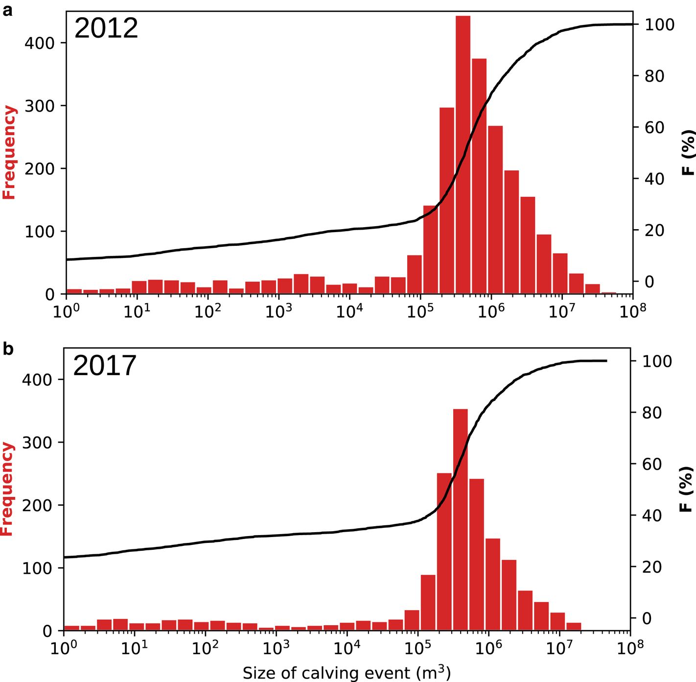
The modelled calving behaviour at Store is seen in Figure 8, which shows that the distribution of icebergs by size in both years is quite similar, with a distinct modal peak in the 3–5 × 10⁵ m3 range. Our model produces 2571 calving events larger than the cut-off size of 1 m3 in 2012 and 1677 similar events in 2017, with a mean size of 1.8 × 10⁶ and 1.1 × 10⁶ m3, respectively. Of these events, 53% (2012) and 59% (2017) are of a size of 105–106 m3, representing 13 and 24% of total calving volume loss, respectively. The largest events (>106 m3) account for 29 and 22% of the total number of events in 2012 and 2017, although a much larger fraction in terms of volume: 87 and 76%, respectively.
Histograms (red bars) and cumulative distribution functions (black line) of modelled calving events at Store by size in (a) 2012 and (b) 2017. Note similar distribution in both years.
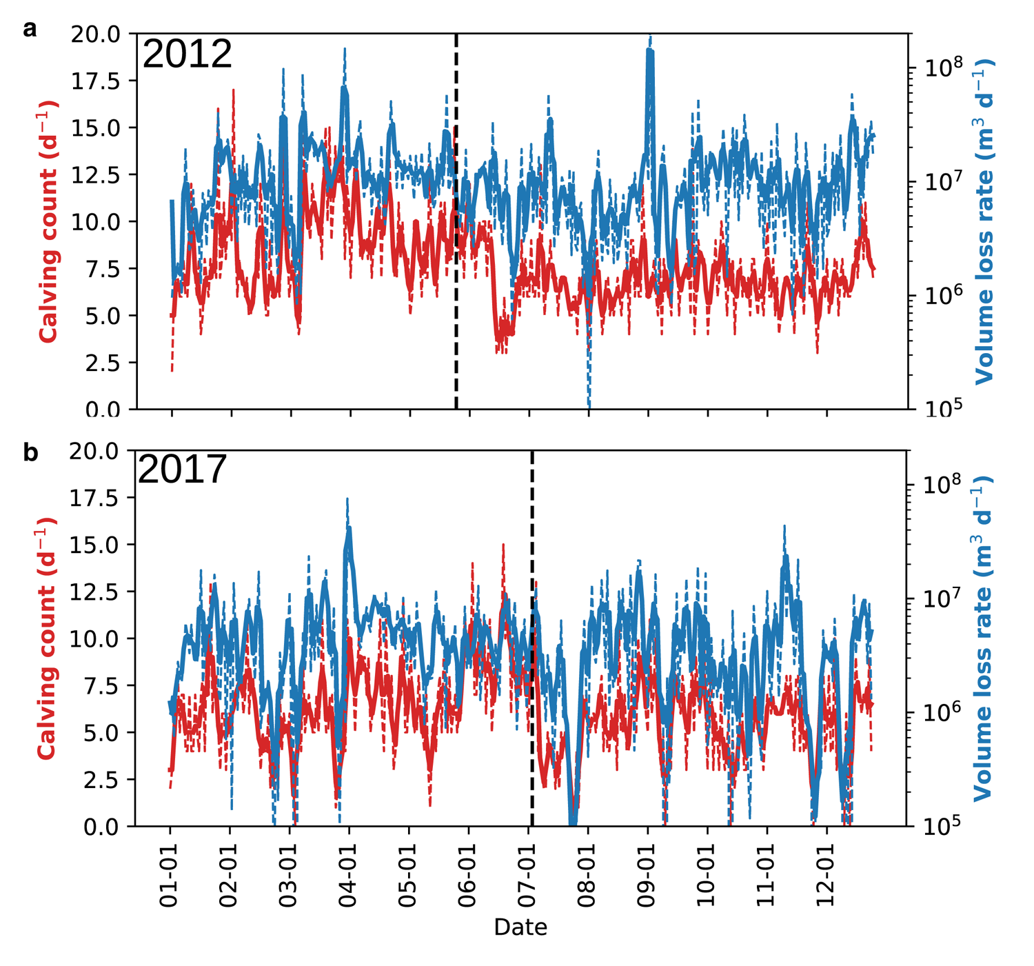
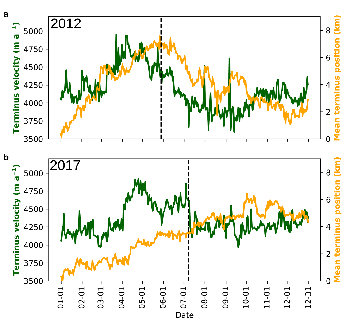
Both 2012 and 2017 show large day-to-day variability in their modelled calving behaviour. However, there is a similar temporal trend in both years (Fig. 9): variable calving at rates of between 5 and 15 events per day in the first part of the year, which drops noticeably to below 5 events per day in the early summer. This is defined as the second week of June in 2012 and the first week of July in 2017. In 2017 (Fig. 9b), this drop coincides with the observed and modelled break-up of the proglacial mélange on 8 July, but, in 2012 (Fig. 9a), it occurs about 3 weeks after the modelled mélange break-up. In 2012, velocity drops from 4300 to 4100 m a−1; in 2017, the drop is from 4600 to 4200 m a−1 (Fig. 10). The controls on this are considered in Section 4. This interplay of velocity and calving also influences the terminus position (Fig. 10) – both years show advance in the terminus through to modelled mélange break-up. In 2012, the modelled terminus advances several kilometres until 29 May, after which it retreats as both velocity and calving rates decline. In 2017, the terminus advances at a slower rate throughout summer and the retreat starts in September. While calving activity drops to ~5 events per day on average when the melt season starts, both years show a return in activity, with ~10 events per day on average in the late summer (July in 2012; August in 2017). Velocity continues to decline in this period in 2012, reaching a minimum of 3700 m a−1 in the first week of September. The terminus consequently retreats to a position only 1 km advanced from that at the start of the simulation, reaching this minimum at the end of November. In 2017, the velocity remains unchanged at ~4200 m a−1 with no further decline, which accounts for the less-marked drop in calving rates that year and the stable terminus position throughout autumn. By the end of the year, however, both simulations show an upwards trend in calving activity, moving back towards 10–15 events per day, which can be linked to the upwards trend in velocity occurring at the same time. In both years, the ice velocity increases to ~4250 m a−1 which is similar to the initialised velocity in each run. As such, in 2012, a small re-advance is seen in December, with the terminus returning to the 3 km mark. In 2017, however, the uptick is smaller and the terminus remains at its autumnal position around the 4 km threshold.
Time series of modelled calving at Store for (a) 2012 and (b) 2017. Red lines show the rate of calving event occurrences per day; blue lines show the volume loss rate per day. The solid lines show the 3 d moving average; the dotted lines show the actual daily totals. Vertical black lines show the timing of mélange break-up. The large volume peak in panel (a) is the result of several large calving events happening to coincide, rather than one anomalously large event.
Average terminus velocity (green line) and position (yellow line) at Store in (a) 2012 and (b) 2017. Note how higher velocities are associated with a lagged terminus advance and lower ones with a lagged retreat.
4. Discussion
This section discusses the results presented in the previous section. Section 4.1 deals with the behaviour of the fully coupled model. Section 4.2 then considers model limitations, particularly with regard to a comparison between modelled and observed calving at Store.
4.1. Fully coupled model behaviour at Store
A highly variable calving activity, with significant day-by-day and week-by-week differences in both 2012 and 2017, is a unique feature of our fully coupled model (Fig. 9). Our results provide theoretical insights into the complex nature of the interaction between ice flow, terminus position, basal hydrology, plume melting and calving. The characteristic features in our model may thus inform causal relationships and behaviour, which have so far not been modelled as directly or explicitly as we do in this study. Our findings therefore provide a quantitative framework for interpreting or inferring processes and mechanisms that control marine-terminating glaciers.
The key factor within the subglacial hydrological system that controls velocity, and therefore also calving, is the extent of channelisation (Fig. 2). As noted in Section 3.1, our 2012 simulation shows a declining trend in basal water pressure in the first part of the melt season (Fig. 6), from May to mid-August, suggesting that the modelled degree of channelisation is sufficient to begin the transition to a widespread efficient drainage system at Store, as has been theorised to occur elsewhere in Greenland (Sole and others, Reference Sole2011; Sundal and others, Reference Sundal2011; Tedstone and others, Reference Tedstone2015; Davison and others, Reference Davison, Sole, Livingstone, Cowton and Nienow2019). However, the basal water pressure still remains higher than in winter (Table 2). In 2017, by contrast, the decline in basal water pressures is more limited (Fig. 6), because channel growth and the extent of channelisation are much reduced (Table 2, Fig. 3, cf. Fig. 2). This limited channelisation also explains why surface-melt spikes in September 2017 produce a much larger response in basal water pressure than in 2012 – the channelised system in both years has started to decay by this point (Fig. 5), but the more-developed 2012 system remains better able to accommodate higher melt inputs and consequently dampens the basal water pressure fluctuations.
Considering the model's performance against observations, the modelled 2017 situation in September has some similarities to the observed behaviour at the western margin of the GrIS in response to a week of warm, wet weather in late August–early September 2011, when unusually high surface runoff (from melt and precipitation) led to basal water pressure exceeding ice overburden pressure (reaching 101%) at site R13 in a borehole 13 km inland from the margin (Doyle and others, Reference Doyle2015). In our model, the domain-averaged basal water pressure reaches 112% of ice overburden pressure very briefly in September 2017, but is otherwise in the 80–99% range.
Comparing model and observations more specifically in a localised area (the area downstream of S30, shown in Figs 2, 3), we see that the model's coupling produces a realistic behaviour in velocity terms in 2012, given that GPS records of ice flow at site S30 have shown significant speed-up events in which ice flow transiently increases from average flow speeds of 630–650 m a−1 to >1000 m a−1 over the course of intense melt events lasting a few days (Doyle and others, Reference Doyle2018). Our model reproduces similar short-lived peaks in velocity (Fig. 2). Our model also reproduced basal water pressures close to the overburden pressure as observed during summer months in this region: Doyle and others (Reference Doyle2018) report basal water pressures of 92–97% of the ice overburden in July and August, which is similar to our modelled basal water pressure peaks of 91–92% of ice overburden during summer. Prior to the onset of melt, the basal water pressures in the model are considerably lower (≈5.5 MPa or 65% of ice overburden, Fig. 2); however, this may stem from model initialisation or an absence of distributed basal drainage, which exists at this time in reality. Our modelled hydrological system is therefore qualitatively consistent with the predominantly inefficient drainage inferred from borehole observations at site S30 (Doyle and others, Reference Doyle2018), which is located in-between two major subglacial drainage pathways and therefore outside the main channelised network (Cook and others, Reference Cook, Christoffersen, Todd, Slater and Chauché2020). However, our model indicates that the region immediately downstream of S30 (Fig. 2) sees more channel growth than the S30 borehole site itself (see Fig. 3 for location). Overall our model clearly shows that channelised basal drainage systems can form beneath Store, and we therefore suggest that tidewater glaciers generally may be able to develop similar systems.
This channelisation control on velocity is confined to the region where the channelised network waxes and wanes seasonally, which means it excludes the terminus region (<10 km from calving front), where channels exist continuously year-round, as well as the interior region (>40 km inland of the calving front), where channels physically cannot form. According to our model, the terminus should contain large channels with cross-sectional areas on the order of hundreds of square metres or more in summer (Figs 3a, d) and persisting throughout winter (Table 2). Hence, channelisation extends inland, starting from the terminus region when runoff first sets in, which occurred early (April) in 2012 and much later (June) in 2017. The corresponding terminus velocity peak (Fig. 7) is mainly a response to pressurisation when these winter channels start to receive runoff (Fig. 6a), although there is also a contribution from higher driving stresses due to winter accumulation thickening the terminus. Inland, however, where the channel network is not present year-round, the modelled velocity variations are predominantly a response to channelisation (Fig. 2). As runoff then increases into summer, however, the terminus velocity declines as the channel network develops and becomes increasingly efficient (Fig. 3), with modelled velocity reaching a minimum in September. As the channelised system subsequently decays, velocity increases through to the end of the year, reflecting the return of a higher-pressure, more distributed system. This matches up with the Type 3 behaviour (midsummer slowdown with a winter rebound in velocity) and posited cause described by Moon and others (Reference Moon2014), which they observe at Store in 2012, providing further validation of the fully coupled model's ability in replicating Store's behaviour.
The pattern of terminus velocity in 2017, however (Fig. 7b), is more reminiscent of Type 2 behaviour (stable velocity from late summer through to early spring, with an early-summer velocity peak) according to the classification of Moon and others (Reference Moon2014). In this simulation, we obtain an early-melt-season (June) velocity peak at the onset of runoff (Fig. 6b), before a return to lower velocities, similar to the pre-melt velocity, unlike in 2012, where summer velocity drops below the start-of-year values (Fig. 7a). The reduced model channelisation in 2017 (compared to 2012) explains this – the initial runoff expands the channels beneath the terminus enough to manage the increased quantities of melt, but subsequent runoff is not enough to build a truly efficient channelised drainage system, meaning the subglacial environment, even at the terminus, remains in an intermediate, partly-channelised state that maintains higher basal water pressures (Fig. 7) and therefore also higher ice velocities. Our simulations of ice flow therefore explain the observed heterogeneous nature of tidewater-glacier behaviour, both temporally and spatially (Csatho and others, Reference Csatho2014; Moon and others, Reference Moon2014). This feature of our model is consistent with recent observations showing tidewater glaciers that have switched from one apparent type to another or even display both traits simultaneously (Vijay and others, Reference Vijay, Khan, Kusk, Solgaard, Moon and Bjørk2019).
However, in both 2012 and 2017, we model an increased average basal water pressure across the model domain in summer, so, even when the modelled hydrology becomes efficient in 2012, the model domain, as a whole, is experiencing higher basal water pressures compared to the preceding winter. This is due to surface melt extending inland to regions where channel development is suppressed (Figs 3c, f) owing to the low surface slope, evolving thickness and velocity of the ice (Dow and others, Reference Dow, Kulessa, Rutt, Doyle and Hubbard2014). This feature of our model may explain why previous studies have observed interannual increases in ice flow in the interior of the GrIS (Doyle and others, Reference Doyle2014), while flow at lower elevations in the same land-terminating catchment in western Greenland slowed down (van de Wal and others, Reference van de Wal2008; Tedstone and others, Reference Tedstone2015) due to the easier formation of channels under thinner ice. The absence of detectable slowdown in this land-terminating region, when looking specifically at winter velocities (Joughin and others, Reference Joughin, Smith and Howat2018), shows that decadal slowdown is almost exclusively a result of peak channelisation in late summer. Our model of a marine-terminating glacier shows that subglacial channels that grow larger than 1 m2 typically close up over the course of <1 week when runoff ceases and that they generally vanish in winter, with the exception of the terminus region. The model also shows that the state of the subglacial drainage system at the end of each simulation is nearly identical (Figs 3a, d; Table 2), despite large differences in the size and configuration of channels during the preceding summer seasons. This shows that a significant enlargement of the channelised system during the record-high-melt year of 2012 did not increase the basal drainage efficiency of the subsequent winter. This suggests that fast-flowing tidewater glaciers like Store do not possess the long-lasting channels hypothesised to stabilise the land-terminating ice margin (Sole and others, Reference Sole2013; Tedstone and others, Reference Tedstone2015). Our model also does not support the hypothesis of large-scale dewatering of the bed lasting into winter owing to channel formation in summer (Hoffman and others, Reference Hoffman2016). This is both due to reduced channelisation and the reduced importance of basal friction (as opposed to lateral friction) in controlling ice motion.
This study shows that the channels beneath Store may have extended 41 km inland in 2012, which is less than the 55 km reported previously when the GLaDS model was not coupled with the flow of ice (Cook and others, Reference Cook, Christoffersen, Todd, Slater and Chauché2020), though the extent for 2017 is nearly identical (29 compared to 30 km). The more restricted inland extent of the channelised system in 2012 in this study is due to the coupling between the hydrology and ice flow allowing the higher basal water pressures under the thicker ice inland to feed back into higher ice velocity, generating localised thickening as ice velocities downstream drop, increasing channel closure rates and consequently suppressing channel formation. Higher velocities inland caused by higher basal water pressure also lead to greater rates of cavity opening in the model, increasing water storage in the sheet, further reducing channel growth. Cavity closing is also suppressed by the lower effective pressure (Werder and others, Reference Werder, Hewitt, Schoof and Flowers2013). The same processes operate in 2017, but there is less of an effect because there is a smaller meltwater input to grow channels, especially in the interior far inland. These results show that ice flow is a critical component of the basal hydrological system and that previous work based on hydrological modelling alone (Banwell and others, Reference Banwell, Willis and Arnold2013, Reference Banwell, Hewitt, Willis and Arnold2016; de Fleurian and others, Reference de Fleurian2016; Cook and others, Reference Cook, Christoffersen, Todd, Slater and Chauché2020) may have over-predicted the ability of channels to form and the extent to which channelised networks grow. Otherwise, however, from a purely hydrological point of view, there is remarkable agreement between the subglacial system modelled in our previous work (Cook and others, Reference Cook, Christoffersen, Todd, Slater and Chauché2020) and the one modelled in this study. This suggests uncoupled hydrological models may give a sufficiently accurate representation of subglacial hydrology under thinner, marginal ice, but lack the processes necessary for accurate modelling under thicker ice inland.
As the foregoing discussion makes clear, the fully coupled model is successful in producing realistic hydrology–velocity coupling and behaviour at Store. This then has an impact on calving at the terminus. Our results show that mélange break-up in our model is not the primary driver of the modelled change in calving rates, but that this change is being largely controlled by runoff and the development of the subglacial hydrological system. This does not mean mélange break-up has no effect on calving, but the fully coupled model results show that hydrology-driven velocity changes at the terminus can be equally, or more, important. This hydrological control was not captured in previous models of Store, either because hydrology was not a model feature (Morlighem and others, Reference Morlighem2016; Todd and others, Reference Todd2018, Reference Todd, Christoffersen, Zwinger, Råback and Benn2019) or because hydrology was not coupled to ice flow (Cook and others, Reference Cook, Christoffersen, Todd, Slater and Chauché2020). We note, however, that mélange buttressing is applied with a back-stress of 45 kPa over a thickness of 75 m in this study, which is consistent with estimates by Walter and others (Reference Walter2012) for Store, although lower than the values of 120 kPa and 140 m used by Todd and others (Reference Todd2018) based on a UAV study of the mélange at the terminus. This difference in model set-up explains why our model shows a more subdued response to mélange formation and break-up compared to previous work (Todd and others, Reference Todd2018), and we would expect mélange buttressing to make a larger contribution to the seasonal characteristics of Store if its back-stress is higher than the values we have assumed here. With a more detailed study of the effect of mélange being beyond the scope of this study, we refer to previous work in which the sensitivity of calving to variation in mélange back-stress was explored, including values similar to those used here (Todd and others, Reference Todd, Christoffersen, Zwinger, Råback and Benn2019).
Whereas previous work posited a link between plume melting and calving at Store (Todd and others, Reference Todd2018, Reference Todd, Christoffersen, Zwinger, Råback and Benn2019), we find the hydrology-induced changes in terminus velocity to exert a stronger control on calving when plumes are modelled physically. This finding stems from the implementation of subglacial hydrology and buoyant meltwater plumes, which makes ice velocities in the model subject to variations in basal drainage efficiency and terminus undercutting controlled by the subglacial discharge. However, it is possible to link plume activity to individual calving events in the model, as shown in Figure 11. This displays two examples of plume activity on the northern side of the calving front. The first example (Figs 11a–e) shows the removal of a small promontory during 28–31 March 2012. The winter discharge from basal melt forms a relatively strong plume with melt rates of 2 m d−1 in the vicinity of the promontory, weakening it over several days and leading to eventual calving. The second example (Figs 11f–j) shows similar behaviour at the same part of the calving front, with stronger plumes (melt rates over 3 m d−1), occurring between 15 and 18 July 2012. This sequence of events is consistent with plume-triggered calving at tidewater-glacier termini (Benn and others, Reference Benn, Cowton, Todd and Luckman2017), allowing us to be confident that the fully coupled model is indeed reproducing realistic tidewater-glacier behaviour. A real equivalent occurring at the approximate same location at Store is shown with time-lapse photographs in Figure 12.
Examples of plume-calving interaction in the 2012 simulation. Figure (a) shows the modelled terminus of Store on 28 March. The red box indicates the area of interest, zoomed in and centred on for a day-by-day view in (b–e) – see how a promontory has calved off. Figure (f) shows a second example of this process happening in summer, with day-by-day views in (g–j). Note higher plume melt rates in and around the promontory that calves.

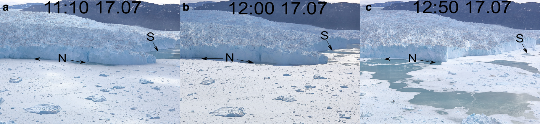
Example of observed surfacing plumes and promontory collapse at the terminus of Store from 17 July 2017. Figure (a) shows terminus at 11:10; (b) at 12:00; and (c) at 12:50. The arrows marked ‘N’ and ‘S’ denote plumes surfacing in the northern and southern plume hotspots, respectively; in panel (c) the southern plumes are much less visible and the two separate northern plumes have joined up. Photo is taken from northern side of fjord looking southwards. Photo credit: A. Abellan.
Considering calving-front plumes further, a notable finding here is that the distribution of plume melt across the terminus is far more uniform in 2017 than in 2012 (Fig. 4). This key feature in our simulations reflects the impact of reduced channelisation at the terminus, with fewer and smaller channels forming ephemeral points of discharge along the terminus in 2017. Maximum melt rates in 2012 are higher, and their impact is localised and much more concentrated; whereas the lower melt rates present in 2017 are evenly spread across the calving front. This general pattern corroborates well with Slater and others (Reference Slater, Nienow, Cowton, Goldberg and Sole2015); however, we model overall higher total melt (by 28%) from the more channelised situation in 2012 compared to the more distributed case in 2017. Given total runoff is nearly three times higher in 2012 (3.2 × 10⁹ m3) than in 2017 (1.3 × 10⁹ m3), this indicates that the increased localisation of higher melt rates does have a powerful mitigating effect on total direct melt from plumes (though not on calving caused by melt-induced destabilisation of the front). However, this is insufficient to completely balance the impact of these higher melt rates. This, combined with the fact that we model 53% more calving events in 2012 than 2017, tends to support the argument made by Todd and others (Reference Todd, Christoffersen, Zwinger, Råback and Benn2019) that higher localised plume melt rates driven by channel discharge are more important in promoting calving and affecting glacier termini than lower, but more widespread, diffuse-drainage-driven melt rates.
The locations of plumes in our model are consistent with observations. In 2012 (Fig. 4a), our model produces two sites with distinct plume activity, or plume hotspots: one on the northern side of the terminus and one on the southern side, that line up well with the observations of surfacing plume activity at Store (Figs 1, 12). In 2017, the northern plume remains a hotspot for submarine melt, but the southern plume is smaller and less stationary, changing location (Fig. 4b). This shows that the modelled subglacial drainage network has a relatively fixed northern discharge outlet and a more mobile southern discharge outlet.
The plume melt rates found in this study reach maximum values of 14 m d−1. While these maximum rates are similar in magnitude to the ice velocity of ~16 m d−1 at the terminus of Store, the seasonal mean values of the daily maximum melt rates are below 5 m d−1 in both years (Table 2). While plume melting may not be a major determinant of terminus position of fast-flowing outlets like Store (Benn and others, Reference Benn, Cowton, Todd and Luckman2017; Cowton and others, Reference Cowton, Todd and Benn2019), it is worth pointing out that higher plume melt coincides with the cessation of terminus advance and, in some cases, terminus retreat in our model (Figs 5, 10).
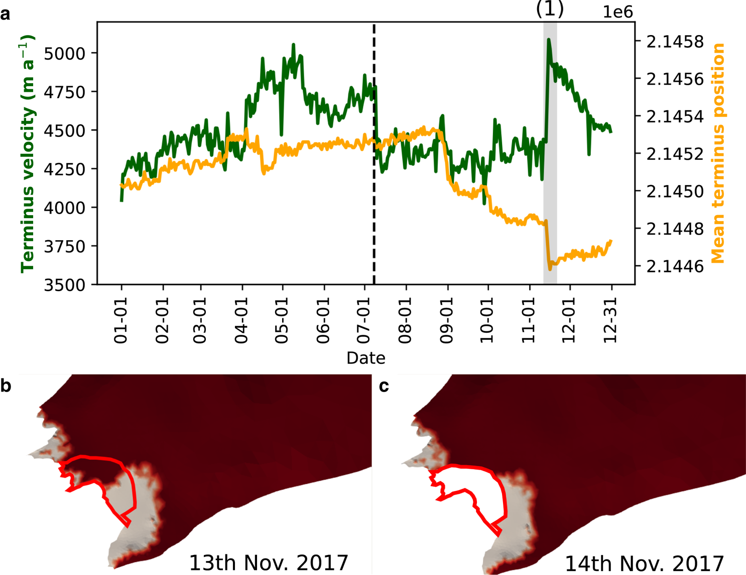
To investigate this further and to test a hypothesis on model limitations (see Section 4.2), we ran two additional simulations identical to those presented in Section 3, except for a quadrupling of the plume melt rate and of the melt rate imposed on the base of the floating ice. Terminus advance is reduced in both years, but particularly in 2017, which begins to exhibit an overall annual terminus retreat (Fig. 13a), lending support to the idea that plume melt rates in excess of terminus velocity can exert a major control on terminus position (Cowton and others, Reference Cowton, Todd and Benn2019). This terminus retreat also allows the model to exhibit a velocity response to calving events (Fig. 13), which is not seen in the previous simulations. Two very large calving events occur in the enhanced melt simulation for 2017: one in late August and the other in mid-November. The first removes only floating ice and henceforth produces only a minor velocity response; the second, however, removes a large area of grounded ice from the centre of the front and this causes the average terminus velocity to increase by over 600 m a−1, the after-effects of which last for over a month until mid-December. It is expected that large calving events involving grounded ice should produce a velocity response (e.g. Benn and others, Reference Benn, Cowton, Todd and Luckman2017) owing to the loss of basal resistance and the resulting steeper surface gradients at the terminus, and this result shows that this behaviour is well-reproduced by our model. As this event only happens near the end of the simulation, it is difficult to draw any conclusions about the effects of such calving on a longer timescale, but it is an indication that marine-terminating glaciers can be sensitive to calving induced by submarine melting.
Calving-velocity response at Store. Figure (a) shows the average terminus velocity and position for 2017 in the quadruple-melt simulation (compare to Fig. 10b). The large calving event (labelled (1)) and associated terminus velocity response are marked by the grey bars in (a). Figures (b) and (c) show the terminus of Store before and after the main constituent of event (1). The calving event is outlined in red. Grounded ice is dark red, ungrounded ice is grey. Note how event (1) removes both floating and grounded ice.
4.2. Comparison to observations and limitations
In this study, we modelled 113 calving events between 5 and 27 July 2017, which is a period during which calving was observed with a terrestrial radar interferometer (TRI) installed at Store (see Cook and others (Reference Cook, Christoffersen, Truffer, Chudley and Abellán2021) for full details of this method). Of these modelled events, 86 were greater than the minimum detectable size of 4000 m3 and the mean size of these events was 730 000 m3. This model characteristic is broadly consistent with the observed mean calving volume of 48 428 m3 which represents only the subaerial fraction of calved ice, which is ~1/10 of the total at Store because the ice has reached floatation at the terminus. While we cannot compare these observations directly with our model because the TRI instrument only captured calving in the northernmost embayment of the terminus, the full-thickness icebergs produced by our model are in overall good agreement with the largest calving events observed in the northern embayment. Our model also captures an increase in these large calving events immediately after mélange break-up, which is similar to observations (Cook and others, Reference Cook, Christoffersen, Truffer, Chudley and Abellán2021).
However, the frequency of modelled calving events is almost two orders of magnitude smaller than the observed number of events, which was 8026 (Cook and others, Reference Cook, Christoffersen, Truffer, Chudley and Abellán2021). With a full-thickness calving criterion, our model cannot reproduce the numerous small calving events (<50 000 m3 in volume) that represent two-thirds of the total observed calving at Store (Cook and others, Reference Cook, Christoffersen, Truffer, Chudley and Abellán2021). As such, our model lacks the processes that cause frequent, small-scale calving, including slabs of ice that topple or fall off when pre-existing fractures weaken the subaerial part of the terminus (Mallalieu and others, Reference Mallalieu, Carrivick, Quincey and Smith2020). Hence, our study shows that a more refined calving criterion is needed to fully capture the range of icebergs produced by calving at major tidewater glacier margins such as Store. Future work may include damaged ice or crevasse ‘memory’, which would allow models to replicate the effects of pre-existing weaknesses on calving.
We also note that the terminus in our model advances more persistently than observed with the TRI and in satellite images. This advance may also limit modelled calving events compared to observations and it is suppressed in our model only when calving is enhanced by quadrupling the plume melt rates. While this may be due to model limitations, it is also possible that submarine melting in reality occurs at higher rates than plume theory predicts, either due to limitations in plume theory (Slater and others, Reference Slater, Goldberg, Nienow and Cowton2016) or because ambient circulation in fjords plays a role, a factor which is currently excluded. T Figure 11 grows a floating ice tongue in the southern part of the terminus (Fig. 11). This floating tongue is supported by observations showing the southern half of the terminus to be afloat (Todd and others, Reference Todd2018); however, the floating tongue in our model is larger than observed. This suggests the model is overestimating the stability of floating ice, possibly for the same reason the terminus advances. One possibility for this is a lack of representation of small calving events, as discussed above.
As a final point, we note that our modelled terminus flows at maximum velocities of 5000 m a−1, which is a little less than observed (≈6000 m a−1). This slower terminus may reflect inadequacies in the underlying slip law, or a failure of the model to fully resolve the small-scale changes and complex basal environment near the terminus.
5. Conclusion
We find that the fully coupled model of Store generally reproduces the characteristic features that describe this glacier, with all model components interacting successfully. Comparison to available observational data shows that the model is capable of reproducing, among others, observed patterns of major calving, terminus velocity and basal water pressures in borehole records. We also demonstrate the high temporal variability of calving activity when the latter is influenced by plume-induced submarine melt. However, our model further makes clear that the terminus velocity of Store is the main synoptic control on calving, because of the strong topographic control on terminus position at this glacier.
The model predicts channelised drainage systems extending 5 km inland all-year-round due to drainage of meltwater produced at the base by frictional heat predominantly. In summer, the channelised drainage system extends up to 29 km inland in a cold year (2017), and 41 km inland in a warm year (2012), which is less extensive compared to earlier work in which the hydrological model was not coupled with ice flow. Our work therefore shows that ice flow influences the storage capacity of the distributed system as well as the ability of channels to form under thick ice in the interior of the ice sheet. However, under thinner, marginal ice, our hydrological results in this study are similar to those obtained with the previous uncoupled model, which suggests simpler models may be sufficiently accurate in such areas.
We additionally show that higher meltwater inputs lead to more channelised drainage at the terminus, and more active plumes with higher melt rates that can have a greater impact on terminus stability and calving. In 2012, when runoff was exceptionally high, we posit that a truly efficient channelised drainage system was present beneath Store, which led to a late-summer slowdown of the terminus, a dynamic response not modelled in 2017. This contrast in behaviour may explain why marine-terminating glaciers elsewhere in Greenland have been observed to seemingly switch from one dominant type linked to an oceanic control through calving to another dominant type linked to atmospheric control through hydrology. However, subglacial water pressures still increased inland in 2012, pointing to the potential for velocity declines at the terminus to be countered by velocity increases farther inland and upstream.
Overall, we show the spatially variable nature of the coupled ice-hydrology system and its importance in determining the behaviour of the terminus and thus calving. The fully coupled nature of the model allows us to also demonstrate the likely lack of any hydrological or ice-dynamic memory at Store, with both years showing very similar glacier states at the end of the runs.
Acknowledgements
The research was supported by the European Research Council under the European Union's Horizon 2020 Research and Innovation Programme. The work is an output from grant agreement 683043 (RESPONDER). S.J.C. also acknowledges financial assistance in the form of a studentship (NE/L002507/1) from the Natural Environment Research Council. The authors thank Marion Bougamont, Tom Cowton, Donald Slater, Antonio Abellán and Thomas Zwinger for productive discussions, as well as Olivier Gagliardini and Peter Råback for support with numerical modelling and Brice Noël who provided the RACMO data, and Nolwenn Chauché who provided the data for the ambient conditions in the fjord. S.J.C. would also like to thank Fabien Gillet-Chaulet for giving him time to work on the preparation of the manuscript. DEMs provided by the Polar Geospatial Center under NSF-OPP awards 1043681, 1559691 and 1542736.


 Open access