

Introduction
Topographic maps of the landscape hidden below the polar seas and the ice cover of Greenland and Antarctica (Fig. 1) are fundamental to our understanding of the tectonic and geomorphological processes that shape the Earth in these regions. They are also fundamental to our ability to understand the past, present and future behaviour of the ice sheets within the coupled ice–ocean–atmosphere system. Several large compilations of topographic survey data have recently been published and many of the earlier blanks on the map have, to some extent, been filled.
Global bathymetry and surface topography, excluding the ice sheets, updated with Bedmap2 (Fretwell et al. Reference Fretwell, Pritchard and Vaughan2013) and the new Greenland compilation (Bamber et al. Reference Bamber, Griggs, Hurkmans, Dowdeswell, Gogineni, Howat, Mouginot, Paden, Palmer, Rignot and Steinhage2013).

For Antarctica, Bedmap2 (http://www.antarctica.ac.uk//bas_research/our_research/az/bedmap2/) consists of a digital elevation model of the continent’s surface and the subice and submarine bed south of 60°S, plus a seamless grid of ice thickness for the ice sheets and floating ice shelves. It is constructed from satellite and airborne altimetry and the entire archive of Southern Ocean bathymetry and available Antarctic ice thickness measurements collected since the beginning of the scientific era. For ice thickness, 25 million measurements were used, almost all coming from airborne radar surveys. Bedmap2 provides much improved estimates of ice sheet volume and potential sea level contribution and, perhaps most strikingly, our first view of a recognizable landscape of troughs, valleys and mountain ranges, the last continental landscape on Earth to be mapped.
For both Antarctica and Greenland, survey data have been won at considerable expense over the last few decades by ground, airborne and shipborne teams from many nations working in difficult conditions with different goals. This variety of survey goals over time has led to a varied patchwork of measurements from densely sampled, regular grids on a local scale to widely spaced point samples along single survey lines thousands of kilometres long. In Greenland, for example, nearly 300 000 line-kilometres of airborne survey have been flown since 2000, with a particular focus on the detailed mapping of major outlet glacier troughs (Bamber et al. Reference Bamber, Griggs, Hurkmans, Dowdeswell, Gogineni, Howat, Mouginot, Paden, Palmer, Rignot and Steinhage2013). In Antarctica, the hidden landscape remains significantly less well mapped than the surface of the moon and the subglacial topography in many areas is not known well enough to constrain models needed to predict the ice sheet’s future.
Now is a good time to examine how well surveyed the polar regions are, to think about how well such datasets meet the needs of the polar science and related communities, and to consider not just where the biggest blanks remain, but where the greatest need for new data lies. This short overview will address two questions with a focus on Antarctica: i) How well do we know the hidden polar landscapes? And, ii) where should future surveys target to be of greatest use to science?
How well do we know the hidden polar landscapes?
Bedmap2 (Fretwell et al. Reference Fretwell, Pritchard and Vaughan2013) and a new Greenland compilation (Bamber et al. Reference Bamber, Griggs, Hurkmans, Dowdeswell, Gogineni, Howat, Mouginot, Paden, Palmer, Rignot and Steinhage2013) provide grids of bathymetry and ice sheet bed topography at 1 km spacing, interpolated from surveys that typically have very dense along-track sampling (of order 10–100 m) but large distances between tracks (of order 1–100 km, exceeding 200 km in places). The cross-track spacing is markedly non-uniform, thus substantial areas of ocean and ice sheets remain unsurveyed. There are, for example, two large areas of East Antarctica totalling c. 500 000 km2 that have no direct bed measurements. Figure 2 shows the global distribution and density of available bathymetric/ice-bed survey data, highlighting the paucity of data in the southern hemisphere relative to the north, and in Antarctica relative to Greenland. Where Antarctica is surveyed, very few areas have more than one 1-km cell with a measurement in any 20 x 20 km square. Figure 3 shows that within and around Antarctica, the Weddell Sea and the coastal fringe of Wilkes Land are particularly poorly mapped, as are substantial portions of the ice sheet interior, but also striking is the paucity or absence of bathymetry data for the cavities below the ice shelves.
Distribution and density of global bathymetric and ice sheet bed elevation data from published Bedmap2, IBCSO (Arndt et al. Reference Arndt, Schenke, Jakobsson, Nitsche, Buys, Goleby, Rebesco, Bohoyo, Hong, Black, Greku, Udintsev, Barrios, Reynoso-Peralta, Taisei and Wigley2013), IBCAO (Jakobsson et al. Reference Jakobsson, Mayer and Coakley2012), GEBCO (IOC et al. 2003) and Greenland bed elevation datasets. Colours show the number of 1 km grid cells within a 20 km square that contain a measurement of sea- or ice-bed elevation.

Published bed elevation data around Antarctica (Bedmap2, IBCSO and GEBCO datasets). Colours show the number of 1 km grid cells within a 20 km square that contain a measurement of sea- or ice-bed elevation. While some parts of the Southern Ocean are well sampled, sampling of the sea floor elevation below the ice shelves is universally poor. Most have no direct measurements of the sub-ice-shelf cavity.

A focus in recent years on surveying the grounded margins of both ice sheets means that the best-surveyed areas now broadly resolve the more extreme relief found around ice stream and outlet glacier troughs. However, particularly in these areas, thick, fast-flowing ice that is crevassed at the surface and warm at the base remains challenging for radar surveys trying to image the bed. In some cases, particularly with older surveys, areas that have been crossed by survey flights consistently have gaps in the data over the thickest or most crevassed ice (Figs 4 & 5a) because the radar signals used to sound the ice thickness have been attenuated by water in warm ice near the glacier bed, or scattered by surface crevasses (Robin et al. Reference Robin, Evans and Bailey1969). Furthermore, the gridding and interpolation used to generate a continuous surface from such heterogeneous data also introduce artefacts where by failing to capture the fine detail present along survey lines and interpolating over gaps in the data (Fig. 5b & c). These two issues lead to misrepresentation of the bed topography even directly under survey lines and particularly affect the steep-sided, deep glacier troughs with high ice flux that are critical in controlling ice sheet mass balance.
Successfully detected bed elevations from airborne radar surveys (black dots) overlaid on ice flow rates for Bindschadler Ice Stream, Antarctica (Rignot et al. Reference Rignot, Mouginot and Scheuchl2011). The apparent breaks in the survey tracks indicate where the radar systematically failed to detect the bed through the crevassed shear margins, visible in Radarsat imagery (inset).

a. Successfully detected bed elevations from airborne radar surveys overlaid on ice flow rates for Smith Glacier, Antarctica (Rignot et al. Reference Rignot, Mouginot and Scheuchl2011). b. & c. Bed elevation profiles from the two radar survey lines in black in a. The black lines show the full-resolution results, which are continuous except for a data gap in the bottom of the deep trough in c. The blue line shows the Bedmap2 elevations gridded from these data. The detailed form of bed troughs is lost in the gridding process, and interpolation across the data gap may have introduced a bias in bed elevation here.

Where should future surveys target to be of greatest scientific value?
Topographic grids, such as Bedmap2, have several potential uses and each use may have different requirements in terms of resolution and coverage. Numerical models that aim to predict ice sheet flow may require, for example, ice sheet-wide coverage with great detail in bed topography where the flux of ice is large and where the form of the bed is a major control on flow rate, such as in ice stream troughs as they approach the coast, but they may be rather insensitive to substantial relief in the slow-flowing interior (e.g. Durand et al. Reference Durand, Gagliardini, Favier, Zwinger and Le Meur2011). Ice sheet models that aim to reconstruct advance and retreat over glacial cycles, or are used to study ocean circulation at the ice–ocean interface, may require detailed mapping through the sub-ice-shelf cavities and farther out onto the continental shelf (e.g. Pollard & DeConto Reference Pollard and DeConto2009). However, models of subglacial hydrology may require the greatest resolution along water flow paths that stretch far inland (e.g. Carter & Fricker Reference Carter and Fricker2012). The scientific case for new surveys and new topographic grids may not correlate with the filling of obvious blanks in the current map.
Method
To outline the scientific requirements for a future bed map, a survey of Antarctic environmental scientists was conducted. Respondents were asked to describe the broad theme of their research and their requirements for improved topographic data in terms of grid resolution, spatial extent and location (Appendix A). A selection of prominent researchers in the themes of glaciology, oceanography, geology, geomorphology, hydrology, ice core science, glacial isostatic adjustment (GIA) and biology was contacted directly for the survey. These researchers were identified by searching recent publications and by seeking recommendations from others in the respective fields. Researchers were chosen regardless of location; 15 nationalities currently working in 12 countries (UK, USA, Germany, New Zealand, Australia, France, Belgium, Norway, Canada, Japan, Brazil and Denmark).
Methods were employed to avoid bias towards glaciology (author’s field) but it is possible that those in the same field were more likely to respond to the questionnaire. To further counter the risk of bias, the survey was sent to a much larger pool of stakeholders on the community Cryolist mailing service (cryolist.org). Cryolist is ‘an email distribution list for those interested in snow, ice and all things frozen’ that has 1460 subscribers based in at least 36 countries.
Seventy-five expert responses were received (Appendix B), some addressing more than one theme. Figure 6 shows the number of responses in each theme. The majority of responses were from the glaciology, oceanography, geomorphology and geology themes, hence the results are somewhat skewed towards these. However, the Cryolist polling opened up the survey to the broader community of Antarctic researchers; seven responses were from the Cryolist solicitation. The relatively low response from other themes suggests a lower level of interest in new Antarctic bed data.
Responses to the Bedgap survey by research theme (80 from 75 respondents).

The goal of the survey was to establish the demand for new Antarctic bed data (spatial distribution, extent and resolution) and not to assign scientific priorities to the demand, which is beyond the scope of this study. Therefore, the results are presented with no weighting towards any theme other than the simplest metric, the number of responses received.
For each theme, the data requirements are mapped to show their spatial distribution, required resolution (high (1–5 km) or very high (<1 km), medium (5–10 km) or low (>10 km)) and number of responses. The motivation for these requirements, as reported in the surveys, is also described.
Glaciology
In the glaciology theme, demand for improved data is dominated by high (1–5 km spacing) to very high- (<1 km) resolution survey of the lower reaches of fast-flowing ice streams, and the ice-stream/ice-shelf grounding zone (Figs 7 & 8). In most cases, this demand corresponds with areas that have previously been surveyed but at lower sampling density (Fig. 3), and reflects a mismatch between the available data and the requirements of a new generation of ice sheet models that seek to represent all of the relevant stresses affecting fast ice flow and the transition to a frictionless environment as ice goes afloat (e.g. Schoof Reference Schoof2007, Durand et al. Reference Durand, Gagliardini, Favier, Zwinger and Le Meur2011), especially in areas of rapid contemporary change (Pritchard et al. Reference Pritchard, Arthern, Vaughan and Edwards2009). Bed features on the sub-kilometre scale can affect the delicate balance of forces in this environment, and the spatial resolution of complex basal topography is a critical factor in the performance of 3-dimensional, full-Stokes ice stream models (Olga Sergienko, personal communication August 2013). Furthermore, subtle bed features may provide sites for ice shelf regrounding or stabilization of a migrating grounding line. In general, such modelling requires bed and ice thickness data at least at a resolution similar to the ice thickness H, and as fine as H/2 or H/3 under ice streams, though this implies that the resolution does not need to be constant everywhere. Several respondents also requested topographic data at the full along-track sampling frequency (tens of metres) of radar surveys in order to characterize bed roughness in the greatest possible detail.
Glaciology responses by resolution class (35 from 30 respondents).

Glaciology priority areas for high- (1–5 km) and very-high-resolution (<1 km) surveying. AS=Amundsen Sea embayment, EAIS=East Antarctic Ice Sheet, F=Filchner Ice Shelf.

Previously neglected priority areas include the lower ice streams flowing into the Filchner Ice Shelf (major outlets of the East Antarctic Ice Sheet (EAIS) that could be affected by future changes to this shelf; Hellmer et al. Reference Hellmer, Kauker, Timmermann, Determann and Rae2012, Ross et al. Reference Ross, Bingham, Corr, Ferraccioli, Jordan, Le Brocq, Rippin, Young, Blankenship and Siegert2012), the glaciers feeding the Shackleton Ice Shelf, and the continental shelf and little known sub-ice-shelf cavities of the Amundsen Sea embayment (Fig. 8). Additionally, detailed studies of stress-transition areas other than the grounding zone, such as ice divides, ice streaming onset zones and shear margins, would benefit from very high-resolution topographic data because high-stress gradients over short distances are critical here (Martín et al. Reference Martín, Hindmarsh and Navarro2006).
Complementing this demand for high-resolution data is a need for low- to medium-resolution survey (5 km and upwards) over major, hitherto neglected regions in the interior (Fig. 9), particularly over the two ‘poles of ignorance’ previously identified (Fretwell et al. Reference Fretwell, Pritchard and Vaughan2013). This map highlights the perceived need for even basic mapping of much of the Recovery Glacier catchment, with one of the largest and deepest troughs in Antarctica penetrating deep into the East Antarctic interior, and the sub-ice-shelf topography of the Filchner and Ronne ice shelves. Additionally, ice sheet mass balance calculations based on differencing snow accumulation from ice flux to the sea require an ice thickness profile along the full length of the grounding line; uncertain thicknesses contribute significantly to uncertainty in mass balance and, hence, Antarctic sea level contribution (Rignot et al. Reference Rignot, Mouginot and Scheuchl2011).
Glaciology priority areas for medium- (5–10 km) and low-resolution (>10 km) surveying. PI=poles of ignorance, RG=Recovery Glacier, RN=Ronne Ice Shelf.

Oceanography
In the oceanography theme, the greatest need for improved bathymetric data is in the sub-ice shelf cavities and troughs cutting the continental shelf of coastal West Antarctica, plus the Thiel Trough/Filchner Ice Shelf, Totten Glacier and the Larsen C Ice Shelf (Figs 10 & 11); areas of contemporary or predicted rapid ice shelf and glacier change (Hellmer et al. Reference Hellmer, Kauker, Timmermann, Determann and Rae2012, Pritchard et al. Reference Pritchard, Ligtenberg, Fricker, Vaughan, van den Broeke and Padman2012). There is also notable interest in the Ross Ice Shelf cavity.
Oceanography priority areas for high- (1–5 km) and very-high-resolution (<1 km) surveying. The underlying topography is shown in greyscale to highlight the continental shelf break fringing Antarctica. AS=Amundsen Sea, F=Filchner Ice Shelf, L=Larsen C Ice Shelf, R=Ross Ice Shelf, T=Totten Glacier, TT=Thiel Trough, WAIS=West Antarctic Ice Sheet.

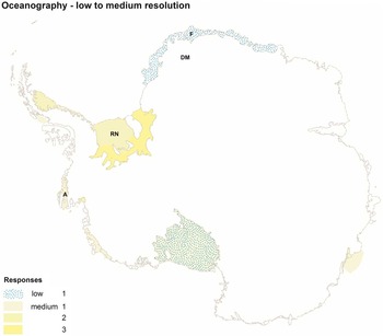
Oceanography priority areas for medium- (5–10 km) and low-resolution (>10 km) surveying. A=Abbot Ice Shelf, DM=Dronning Maud Land, F=Fimbul Ice Shelf, RN=Ronne Ice Shelf.
High and very high-resolution mapping (e.g. swath bathymetry) is in particular demand in the Amundsen Sea embayment, where there is evidence for the incursion of relatively warm and dense circumpolar deep water from offshore of the continental shelf break that flows down glacially-scoured troughs and comes into contact with the thick ice shelves of major West Antarctic glaciers (Jenkins et al. Reference Jenkins, Dutrieux, Jacobs, McPhail, Perrett, Webb and White2010). This is probably the driver of ongoing rapid West Antarctic deglaciation, which is the primary source of Antarctica’s contribution to sea level rise (Pritchard et al. Reference Pritchard, Ligtenberg, Fricker, Vaughan, van den Broeke and Padman2012, Shepherd et al. Reference Shepherd, Ivins and Geruo2012). The arrival and transport of dense, warm water on the continental shelf of the Amundsen Sea and elsewhere is controlled by sills and troughs in the bathymetry, and to understand the transport of this warm water along troughs, ocean models need to resolve mesoscale eddies with a radius of deformation of c. 4.5 km, requiring bathymetric mapping at c. 1–1.5 km. Very detailed mapping at the continental shelf break and landwards is therefore required to predict the future ocean forcing of ice sheet retreat, explaining the demand for extensive higher resolution data (Fig. 12).
Oceanography responses by resolution class (23 from 20 respondents).

Along the coastal fringe of Dronning Maud Land, the continental shelf is narrow and Warm Deep Water lies nearby, though the amount beneath the ice shelves is highly uncertain and only the Fimbul Ice Shelf has detailed sub-ice-shelf bathymetry; even reconnaissance-level data would be valuable along this coast. Other ice shelves with large melt uncertainty in a recent circum-Antarctic melt assessment (Rignot et al. Reference Rignot, Jacobs, Mouginot and Scheuchl2013) include the Larsen C, Ronne, Abbot and western Ross ice shelves, motivating the need for improved survey data at these sites (Figs 10 & 11).
Geology and geomorphology
In the geomorphology theme, the demand is universally for high or very high-resolution mapping, with this demand strongly concentrated on the grounding zones and continental shelves offshore of major glaciers, particularly in coastal West Antarctica. A very high resolution (e.g. from swath bathymetry) is required primarily in order to resolve palaeo-ice sheet bed features that indicate ice flow rate and direction, bed properties, hydrology and former grounding line positions, particularly for the West Antarctic Ice Sheet (WAIS) as it retreated back from its last glacial maximum extent to its current state, a process that may be analogous to present and future retreat (e.g. Graham et al. Reference Graham, Larter, Gohl, Dowdeswell, Hillenbrand, Smith, Evans, Kuhn and Deen2010). Such bed features tend to be concentrated in ice stream-scoured troughs and thus the target areas in Fig. 13 are relatively small. The same features can be observed under today’s ice streams, revealing the link between ice flow behaviour and basal geomorphology (Smith et al. Reference Smith, Murray, Nicholls, Makinson, Aoalgeirsdóttir, Behar and Vaughan2007, King et al. Reference King, Hindmarsh and Stokes2009), but such process-based studies into subglacial landform development have been done only very locally on three ice streams. Further priority targets are identified over grounded ice in Fig. 13.
Geology and geomorphology priority areas. The underlying topography is shown in greyscale to highlight the continental shelf break fringing Antarctica. A=Aurora subglacial basin, E=Ellsworth Mountains, G=Gamburtsev Subglacial Highlands, H=Heritage Mountains, MB=Marie Byrd Land, MF=Moller/Foundation region, PE=Princess Elizabeth Land, S=Shackleton Mountains, V=Vostok highlands, W=West Antarctic Rift System.

Another application for detailed landscape mapping arises along the margins of the Ellsworth, Shackleton and Heritage mountain ranges of West Antarctica (Fig. 13), where geological studies suggest that a similar ice cover has persisted over several glacial-interglacial cycles, but detailed subglacial mapping down to the corrie-scale is needed to understand whether this history is representative of broader ice sheet glaciation or local alpine glaciation.
In the geology theme, further surveying is motivated by the desire to understand better the major tectonic boundaries and rift systems of Antarctica, such as the East Antarctic–West Antarctic boundary in the poorly mapped Moller/Foundation region, the boundary between the deep Aurora subglacial basin (A) and the Vostok highlands (V), the almost unknown Princess Elizabeth and Marie Byrd lands, and the northward extension of the West Antarctic Rift System (Fig. 13). These features are important in, for example, reconstructing supercontinent evolution, investigating long-term ice sheet stability by looking at the landscape links between East and West Antarctica, studying volcano–ice interactions (Corr & Vaughan Reference Corr and Vaughan2008), and studying the role that rifts play in steering and controlling the interplay between grounded ice streams and offshore ocean currents (Bingham et al. Reference Bingham, Ferraccioli, King, Larter, Pritchard, Smith and Vaughan2012). Additionally, detailed survey of mountainous landscapes in the East Antarctic interior (circular, pink regions in Fig. 13) are needed to understand better Pleistocene ice sheet inception and evolution. Similar mapping over the Gamburtsev Subglacial Highlands resolved a preserved alpine landscape of valleys and corries believed to have held the first Antarctic glaciers and to have formed the original core of the present ice sheet (Bo et al. Reference Bo, Siegert, Mudd, Sugden, Fujita, Cui, Jiang, Tang and Li2009).
Hydrology, ice cores, biology and glacial isostatic adjustment
Ice core research requires reconnaissance surveying at medium resolution, focussing on smaller areas at high and very high resolution over domes A, C, F, the West Antarctic divide between the Weddell and Amundsen sea coasts and the crest of the Antarctic Peninsula (Fig. 14), in order to identify sites with deep, old ice that does not experience complex flow or basal melt.
Hydrology, ice cores, biology and glacial isostatic adjustment (GIA) priority areas. The underlying topography is shown in greyscale to highlight the continental shelf break fringing Antarctica. AP=Antarctic Peninsula, DF=dome F, DA=dome A, DC=dome C, RL=Recovery Lakes, SC=Siple Coast, W=Weddell Sea.

Hydrological survey is required at least at reconnaissance resolution over the Recovery Lakes area and at higher resolutions on other ice streams, ranging over spatial scales of entire hydrological basins down to individual channels. Particular gaps currently exist between the pole and the Filchner Ice Shelf, and on the Siple Coast where a very active hydrological system has been observed (Smith et al. Reference Smith, Fricker, Joughin and Tulaczyk2009, Carter & Fricker Reference Carter and Fricker2012), and where radical changes in ice stream flow result from switching of subglacial water drainage paths (Conway et al. Reference Conway, Catania, Raymond, Gades, Scambos and Engelhardt2002).
For studies of biodiversity, biogeography, deep-sea biology and evolutionary history, benthic surveys require lower resolution bathymetry over large areas to identify zones suitable for using fishing equipment, followed by detailed (swath) survey to plan specific sampling profiles. Such studies can also provide evidence of ice sheet history, where formerly open seaways may have provided pathways for species dispersal reflected in contemporary ecosystems (Vaughan et al. Reference Vaughan, Barnes, Fretwell and Bingham2011).
Models of GIA of the Earth in response to ice sheet loading/unloading can be used to infer past ice sheet mass, and rates and patterns of deglaciation; however, past ice sheet extent is poorly constrained in GIA models, particularly along the EAIS margin offshore of the major outlet glaciers. Very high-resolution mapping is needed here for geomorphological interpretation of ice sheet retreat. Furthermore, GIA models are now being coupled to ice sheet models because GIA and gravitational feedbacks can play an important stabilizing role at retreating grounding lines (Gomez et al. Reference Gomez, Mitrovica, Huybers and Clark2010). Marginal ice loss triggers local crustal rebound and gravitational decrease, both factors cause a relative sea level fall locally, which has a positive impact on ice sheet effective pressure and, hence, basal drag. This acts to stabilize marginal retreat, but such modelling, as for ice sheet models alone, requires high-resolution topographic data for the grounding zone and continental shelf.
Cumulative bed topography requirements
Figure 15 shows the combined coverage of bed topography requirements, the sum of responses in all themes. The greatest demand, and requested by all themes except ice cores and geology, is for the lower reaches of Pine Island and Thwaites glaciers in the Amundsen Sea embayment of West Antarctica, already among the best sampled areas in the continent (Fig. 3). Also highlighted here, and common to most themes, is a demand for more data in the Thiel Trough/Filchner Ice Shelf, several areas near the landward margin of the Ronne Ice Shelf in the Weddell Sea sector and a selection of sub-ice-shelf cavities. In particular, the grounding zone junction between ice streams and ice shelves is a priority for oceanographers, glaciologists and geomorphologists. Inland, the poles of ignorance around the Recovery/Support Force glaciers and in Princess Elizabeth Land seaward of the Gamburtsev Mountains (Fig. 9) are prominently of high priority to both the glaciology and geology communities.
The cumulative demand (number of responses) for improved Antarctic bed mapping across all themes. P=Pine Island Glaciers, TH=Thwaites Glacier, TT=Thiel Trough, F=Filchner Ice Sheet, RN=Ronne Ice Shelf, P=poles of ignorance.

What is currently achievable?
Over the grounded ice sheet, bed topography is typically mapped by airborne radar on aircraft operated from Antarctic stations or field camps, or by long-range aircraft based in southern South America. Conducting extensive airborne surveys in the Antarctic deep field is challenging, particularly given the short flying season and the cost of transporting fuel to field depots. As an example, two recent, detailed and large-scale airborne radar surveys operating from remote field camps surveyed boxes of c. 1000 x 200 km and 800 x 600 km respectively in a season, at a line spacing ranging from 5–50 km. This involved surveying 120 000 and 78 500 line-kilometres, respectively, at a (full economic) cost of $50–$100 per kilometre. Although technically and logistically feasible, increasing the resolution to c. 1 km-line spacing over an equivalent area would multiply the flying time and distance by at least five times. Therefore, with current technology, the requirements for improved survey of the grounded ice sheet are achievable but at high cost. Airborne swath radar is being developed that will yield very high-resolution bed mapping along and across track, but the relatively narrow swaths would not overcome the need for closely spaced flight lines.
In the Southern Ocean and neighbouring seas, swath bathymetry frequently delivers very high-resolution (<1 km) data, though notable gaps remain, particularly in the Weddell, Ross and southern Bellingshausen seas, and over the continental shelf of East Antarctica south of Australia (Figs 2 & 3). The Weddell Sea is particularly prone to extensive and prolonged sea ice cover, consistently restricting ship access, and many other continental shelf sea areas are frequently inaccessible due to sea ice and are prone to iceberg hazards (Holland & Kwok Reference Holland and Kwok2012). Therefore, the required improvement in ocean bathymetry is technically feasible but logistically difficult and may take a considerable time to achieve through opportunistic visits in favourable conditions.
The most challenging survey goal is to provide bathymetric mapping of the ice shelf cavities at resolutions of order 1 km, many of which are entirely uncharted (Fig. 3). They can be sounded point-by-point by over-snow active seismic surveys but this is typically too slow to yield more than reconnaissance-level mapping (Determann et al. Reference Determann, Thyssen and Engelhardt1988), even provided that travel over the ice shelf surface is possible, and this is not the case for most fast-flowing ice shelves. Indirect methods are available (e.g. airborne gravimetry (Tinto & Bell Reference Tinto and Bell2011) and analysis of tide model-observation misfit (Hemer et al. Reference Hemer, Hunter and Coleman2006)) but these may be prone to bias (Brisbourne et al. Reference Brisbourne, Smith, King, Nicholls, Holland and Makinson2013) and cannot yield the resolutions required by most respondents to this survey.
The sole alternative at present is multibeam sonar sounding by autonomous underwater vehicles (AUVs) that travel under the ice shelf (Jenkins et al. Reference Jenkins, Dutrieux, Jacobs, McPhail, Perrett, Webb and White2010). The vehicle used in this pioneering study, Autosub3, has a maximum range of 400 km and travels at up to 6 km hour-1. It was deployed up to 60 km under Pine Island Ice Shelf and mapped a 510 km long, 200–300 m wide swath in 94 hours at sea. Ship operating costs in such areas are particularly high, and in this instance, the equivalent line-survey cost would appear to be at least ten times that of the deep field airborne surveys. With this range and assuming ship access to the ice shelf front for deployment of the AUV, all smaller shelf cavities are accessible but only the outer third of the Ross and Ronne–Filchner ice shelves, and the outer half of the Amery Ice Shelf could be reached. Ocean currents and navigation hazards may also significantly limit the potential AUV range. However, new AUVs with much greater endurance have recently been developed and will soon be deployed. From this, we can say that the required sub-ice-shelf bathymetric data coverage and resolution will probably be feasible, but will be more expensive than for surveys of either grounded ice or open ocean bed topography.
Conclusions
The distribution of survey data for the Greenland and Antarctic ice sheets and neighbouring seas shows that Antarctic topography is considerably less well sampled than that in the Arctic, and there remain large areas that are uncharted. Furthermore, even where surveys have been conducted, radar sounding has frequently failed over the deepest glacial troughs and on crevassed shear margins, leaving gaps in topographic data over some of the most glaciologically important areas.
The large gaps in existing topographic data coverage are areas unknown to science and could potentially generate considerable demand for detailed research. Therefore, these must be seen as important targets at least for reconnaissance scale sounding of the bed. However, a survey of 75 experts in Antarctic environmental science (with the majority from the fields of glaciology and oceanography) shows that the most obvious gaps are not necessarily perceived as the immediate priority areas for future survey. Among glaciologists, for example, there is considerable demand for even higher resolution mapping of certain previously surveyed key areas, particularly in the lower reaches of fast-flowing ice streams, and above all in the Amundsen Sea embayment of West Antarctica. This demand stems primarily from the needs of advanced ice sheet models to resolve in detail the three-dimensional stress fields around ice stream grounding zones, which are critical to reproducing large observed changes in ice flux and, hence, ice sheet contributions to sea level change. Concern about potential future melting of the Filchner Ice Shelf has also stimulated a demand for mapping at various resolutions of its previously neglected tributary ice streams. Given existing technology and logistic infrastructure, the data requirements over grounded ice could, in principle, be met by airborne radar survey.
Among oceanographers, demand is strongest for higher resolution data on the continental shelf (including ice shelf cavities) in the Amundsen Sea embayment and, to a lesser degree, the Filchner Ice Shelf and the sea floor adjacent to Totten Glacier in East Antarctica. This is motivated primarily by a need to resolve the topographic features that control ocean circulation at the ice–ocean interface, particularly the arrival of warm waters at depth that increase ice shelf melt. Similarly, geomorphologists universally identified a need for high or very high-resolution data over relatively small areas of current or previous fast glacier flow. This is motivated by the goal of identifying landforms associated with such fast flow, and in particular, of mapping the history of ice sheet behaviour of advance and retreat over the continental shelf through previous glacial cycles, a goal echoed by those attempting to improve GIA and couple GIA-ice sheet models. Detailed mapping of the continental shelf by shipborne swath bathymetry is feasible but greatly constrained by extensive and unpredictable sea ice cover. Mapping of ice-shelf cavities is particularly challenging and expensive but, with the development of new AUVs, may soon be feasible at high resolution for all ice shelves.
For hydrologists and ice core researchers, precisely targeted, detailed surveys are needed to, respectively, resolve and avoid water at the bed, though these should be guided by preliminary, lower resolution reconnaissance, an approach similar to that required by marine biologists studying continental shelf ecosystems. Lower resolution reconnaissance is also suited to the wide ranging surveys required to flesh out the picture of supercontinent formation and breakup, rifting, mountain building and ice sheet inception of interest to a number of geologists in this survey.
To conclude, the known requirements for Antarctic topographic data of all of the science themes addressed here are not fully met by the presently available data. These unmet demands are hindering progress in, for example, predicting the dynamic response of the ice sheet to ocean forcing and, hence, our understanding of how the Antarctic ice sheet will respond to a warming world. However, the required data coverage and resolution could be achieved in the open ocean and over grounded ice, and may soon be achievable under even the largest ice shelves if improved AUVs successfully penetrate the deep sub-ice-shelf cavities.
Acknowledgements
I would like to thank the 75 contributors to the Bedgap survey, and also Professor David Sugden and an anonymous reviewer for their supportive and constructive comments on this manuscript.
Appendix A. Bedgap questionnaire
Your name:
Thinking about future priorities for Antarctic survey, I’d like to ask about your highest-priority requirements for a bedmap-type product of subglacial and submarine topography. Very detailed surveying everywhere would be nice but of course in practice we need to think about targeted campaigns.
Specifically, I’d like to ask about the resolution, the spatial extent and the location of where you would like to see improved surveying.
For example, if you are interested in ice stream grounding line processes, your priority may be for very fine detail in a zone close to the Thwaites Glacier grounding line or, for broader studies, perhaps somewhat improved detail for all Antarctic grounding zones. In geomorphology, the priority may be for an improved survey of a subglacial mountain range that resolves valley and cirque features. Oceanographers may prioritize sub-ice-shelf cavities or troughs in the continental shelf. Ice corers may want to target the deepest basins at relatively low resolution.
1) In terms of bed topography, what sampling does your work require? i.e. how detailed does the topographic grid need to be to capture the features important to your research? Please give a value in km (e.g. 0.1 km, 2 km, 10 km, etc.).
2) Approximately what size of area would you need these data over? This doesn’t need to be an exact measure, it could be a rough box e.g. 20 x 20 km, 100 x 100 km, or 500 x 1000 km.
3) Where would you put this survey? To answer this, you can either centre it on a latitude/longitude coordinate or define it by a recognized geographical name so I could work out where to put it on a map. Here are some examples:
-
i) Seas or sea areas: Weddell Sea continental shelf, Weddell Sea deep ocean.
-
ii) Sub-ice-shelves: Wilkins, or a grouping such as eastern Antarctic Peninsula shelves.
-
iii) Ice streams/glaciers: lower Thwaites Glacier, or a grouping e.g. Siple Coast Ice Streams.
-
iv) Interior: Recovery Lakes, Wilhelm II Land.
4) What is the theme of your research? e.g. ice stream dynamics, ice shelf oceanography, subglacial hydrology, geomorphology, ice cores.
Appendix B. Contributors to the Bedgap survey


 Open access