

Mathematical Symbols

1. Introduction
Over the past decade, the concept of a deformable glacier bed has fuelled innumerable investigations particularly with respect to its role in basal sliding (e.g. Reference KambKamb, 1991; Reference Blake, Clarke and GérinBlake and others, 1992; Reference Iverson, Hanson, Hooke and JanssonIverson and others, 1995; Reference Engelhardt and KambEngelhardt and Kamb, 1998), subglacial water drainage (e.g. Reference Walder and FowlerWalder and Fowler, 1994), sediment transport (e.g. Reference AlleyAlley, 1991; Reference BoultonBoulton, 1996) and landform development (e.g. Reference Boyce and EylesBoyce and Eyles, 1991; Reference HindmarshHindmarsh, 1998a, b). An interesting question which arises is this: How is the basal traction distributed under a glacier? To answer this requires a knowledge of the spatial extent of basal ice that is in contact with the bed. The contact interface can support stresses. For a soft bed, storage or transport of water can occur where the ice and till have separated, as well as by percolation within the till (and subsequent advection); deformation of till may also contribute to glacier motion. Hence, contact regions have critical dynamical and hydrological implications. The difficulty lies in describing how their nature and distribution vary with time. Given that these may be spatially variable, determination by field measurement may require a large number of sampling points (e.g. boreholes); yet theories that are constructed to focus measurements and aid their interpretation have been conspicuously few.
Evolution of the regions of contact between ice and till is the net result of various processes. For instance, the ice–till interface may recede (in terms of areal coverage) when bed sediments are eroded by an expanding subglacial drainage system. But generally, the interface itself is in continual motion as the two materials deform. This occurs in response to the heterogeneous stress distribution at the glacier bed, induced, for example, by the presence of subglacial channels. Our aim in this paper is to calculate such motion.
Even in the simplest case, the proposed calculation is difficult because it requires simultaneous solution of flow problems in both the ice and the sediment. (They cannot be solved independently.) This is further complicated by the rheologies involved. Thus, in this preliminary work, we shall make several assumptions to facilitate our analysis; these concern especially the detailed mechanical and hydraulic behaviour of till. This approach should not alarm experimentalists, however, as the emphasis is not on any definite numerical predictions, but on properties of the coupled deformation of ice and till that deserve further attention, especially with sliding and drainage theories in mind. Indeed, we argue that coupled deformation should not be neglected in the dynamical description of glaciers overlying a soft bed.
2. Background
2.1. Basal sliding
A classic description of the extent of ice–bed contact is encountered in the theory of basal sliding over a hard bed with non-uniform topography (Reference FowlerFowler, 1987; Reference KambKamb, 1987). Here, consideration is given also to the water flow that occurs in the resulting system of linked cavities (Reference WalderWalder, 1986; Reference KambKamb, 1987). The proportion of decoupled area (cavities) is controlled by the rates of sliding, melting (due to dissipative heating) and deformation closure of the ice. This ratio is important because it determines the partitioning of normal/shear stresses acting at the bed.
The current investigation provides a constituent for a soft-bed extension of the theory, in which relevant processes include ice and till deformation, as well as melting (of ice) and erosion (of sediment) in the decoupled region. Till sliding (relative motion at the ice–till interface) is also possible, but its effect is excluded here. In this paper, only deformation is investigated. The decoupled region may correspond to a locally thickened water film, a subglacial cavity or a water channel, but distinction between these is not necessary in the present context. We shall refer to it as the “channel” or “channel–cavity” in the following. Basic inputs for calculating deformation include the overburden stress due to the ice above, and drainage parameters for this channel–cavity, which we shall take as prescribed.
2.2. Subglacial water transport
Several authors have sought ice-deformation rates near subglacial channels, motivated by the need to describe subglacial drainage regulation. The elementary theory considers a balance between the velocities of melting and creep closure at the channel walls (Reference RöthlisbergerRöthlisberger, 1972; Reference NyeNye, 1976). A soft bed introduces new factors when determining the analogous theory, since deformation, erosion and deposition of sediment presumably have at least some effect on channel form and network configuration.
Extensive till deposits of the order of decimetres or more in thickness have been inferred at a number of locations beneath contemporary glaciers and ice sheets (e.g. Reference Alley, Blankenship, Bentley and RooneyAlley and others, 1986; Reference Rooney, Blankenship, Alley and BentleyRooney and others, 1987; Reference Blake, Clarke and GérinBlake and others, 1992; Reference Murray and PorterMurray and Porter, 1994; Reference Iverson, Hanson, Hooke and JanssonIverson and others, 1995). Drainage can provide an efficient mechanism whereby till sediments are evacuated. Specifically, if drainage is predominantly channelized, then the sediments can interact with water flow through uptake as bedload and suspended load. Channels tend to enlarge as a result, but in the case where the till is water-saturated and subjected to an overburden stress higher than the channel flow pressure, this would be opposed by the inward creep of sediments into the channels.
Since drainage network survival depends on the maintenance of individual pathways, the counterbalance described above, namely, that between creep deformation, which causes closure, and fluvial erosion, which causes opening, provides a plausible starting-point for analyzing soft-bed channelized drainage. (This is additional to the melting vs closure competition in the ice.) This idea was first introduced by Reference Boulton and HindmarshBoulton and Hindmarsh (1987), and subsequent modelling by Reference Walder and FowlerWalder and Fowler (1994) examined the properties of steady flow, where an exact balance is assumed. In their proposed theory, sediment creep motion is a prerequisite for steady drainage to occur; the closure velocity controls the cross-sectional shape of the “canals”, and hence their drainage characteristics. These results have since been supplanted by those of Reference NgNg (2000). However, he showed that a knowledge of till deformation is still required for describing the sediment budget and drainage organization, particularly in the downstream direction of the canals. This conclusion would be unaltered in a time-averaged description of drainage over soft bed which attempts to capture the irregular nature of flow-path formation and evolution — such as that suggested by Reference HindmarshHindmarsh (1997). Some quantification of overall deformation rates is therefore necessary.
2.3. Determining deformation rates
Previous calculations of ice/till deformation adjacent to subglacial conduits illustrate well the effect of non-linear rheology. These include the following:
-
(i) Reference NyeNye’s (1953) derivation, based on Glen’s law, which considered the creep of ice near a (long) cylindrical conduit.
-
(ii) Reference AlleyAlley’s (1992) model of the behaviour of deformable till adjacent to a subglacial channel. He showed that sediment flow with a Coulomb–Bingham rheology would be limited to a narrow zone by the channel margins, and that this process leads to pinch-out of the till over bedrock.
-
(iii) Reference Walder and FowlerWalder and Fowler’s (1994) canal model, which employed modified forms of Nye’s result for both ice and till. Their full derivation of the closure velocity of a till channel, assuming a Boulton–Hindmarsh type rheology for the sediment (see section 3), is reported by Reference Fowler and WalderFowler and Walder (1993).
This brings us to the main point of the paper. None of these models, which consider ice and till flow independently, can describe coupled deformation of both materials. The adopted description for each material has been derived on the basis that the other material was either stationary or absent altogether, but this is not generally the case. This poses a significant problem when building consistent sliding and drainage theories for a soft bed. Herein, we present a pilot investigation of the coupled deformation. Most crucially, we allow the interface outside the channel–cavity to be freely mobile. In mathematical terms, such mobility can be accounted for by applying continuity conditions for stress and velocity across the interface.
With the ice, sediment and channel, it is necessary to consider a more realistic geometry than has been analyzed in (i) to (iii). But given additional rheological complications, it seems reasonable to begin the modelling with the bare essentials. A simple situation is where the principal ice-flow direction (and also the channel axis) is “out-of-paper”, which allows us to formulate plane flow equations in two dimensions. The channel is assumed to have high aspect ratio, i.e. it is wide and low. The deforming thickness of till is prescribed. Also, we assume the simplest workable models of rheology, at least initially. While these would obviously limit the applicability of our model, extensive computation is avoided. And although this arrangement is by no means general, it provides a basis for extension, particularly to the three-dimensional problem.
Rheology-related issues are covered in section 3. The investigation then consists of two parts. First (in section 4), we solve a mathematical model that describes linear coupled flow, taking constant (effective) values for ice and till viscosities. This exercise is informative, because the till viscosity is particularly sensitive to till type and basal (e.g. drainage) conditions and lies in a range that spans many orders of magnitude, even though each viscosity value (for ice or till) may vary spatially. Therefore, our initial interest is not in their precise values but in their ratio. If typical ice and till viscosities are η I and η T, respectively, then the resulting deformation is examined for η I ∼ η T, and for the asymptotic limits associated with η I ≪ η T and η I ≫ η T. We also consider the effect of varying the depth of the deforming-till layer.
Next (in section 5), an assessment is made of the effect of spatially varying viscosity, specifically that of the till, despite uncertainties in modelling its rheology (as will be explained in section 3). We do this by analyzing a steady-state creep model based on Reference Fowler and WalderFowler and Walder’s (1993) formulation for non-linear viscosity till. We use the interfacial stresses/velocities derived in section 4 to represent the general form of the boundary conditions. This model allows us to explore in more detail sediment hydraulics and mechanics near the margins of the channel–cavity. Our deductions will primarily be based on the results of scaling analysis.
Finally (in section 6), our results and their implications are discussed, and we indicate directions for further research and extensions. We should point out that, although the close connection of this work with subglacial drainage will soon become evident, no attempt is made here to promote any particular drainage theory.
3. Modelling till Rheology
Ice is usually treated as a non-linear viscous fluid (obeying Glen’s law, for instance), but the analogous model for till has been rather controversial and demands attention. The current debate focuses on whether a viscous or plastic description is more appropriate (Reference HindmarshHindmarsh, 1997).
The realization that fast ice flow may be caused by a deforming substrate is based on the premise that subglacial till, like other granular materials, undergoes irreversible deformation once a yield stress (τ
c) is exceeded. To describe the subsequent motion, a constitutive relation between stress τ (≥ τ
c) and strain rate
![]() has often been adopted. Some modellers proposed a viscous rheological law of the formFootnote
*
has often been adopted. Some modellers proposed a viscous rheological law of the formFootnote
*
where N is the effective stress in the till (overburden pressure minus pore-water pressure), and a and b are empirically determined constants. The yield stress depends on N also, via the Coulomb expression
where c 0 is cohesion (usually negligible) and ϕ 0 is the internal friction angle of the sediment. When τ > τ c, Equation (1) implies a stress-dependent viscosity given by
The modelled till viscosity then decreases as effective stress decreases.
According to Equation (3), “low” values of a and b (specifically, a ≈ 1 and b ≈ 0) would lead to an approximately constant value of η. The resulting, mildly non-linear, viscous behaviour was much popularized after Boulton and Hindmarsh’s (1987) measurements under Breiðamerkurjökull in Iceland, where they obtained a = 1.33, b = 1.8 and A T = 3 × 10⁻⁵ Pa b −a s−1 as best-fit parameters to the equation
(a special case of Equation (1)). Their yield stress was found to be negligible as compared to the range of applied stress (τ c ≈ 0).
In contrast, laboratory experiments on till samples have indicated a highly non-linear behaviour under deformation, with measured values of τ close to τ
c over a large range of
![]() (Reference KambKamb, 1991; Reference Hooke, Hanson, Iverson, Jansson and FischerHooke and others, 1997; Reference Iverson, Hooyer and BakerIverson and others, 1998). This is in broad agreement with results from geotechnical testing of similar materials, where it is common to express the weak dependence of stress (in geotechnical terms, the “residual” stress) on strain rate by writing
(Reference KambKamb, 1991; Reference Hooke, Hanson, Iverson, Jansson and FischerHooke and others, 1997; Reference Iverson, Hooyer and BakerIverson and others, 1998). This is in broad agreement with results from geotechnical testing of similar materials, where it is common to express the weak dependence of stress (in geotechnical terms, the “residual” stress) on strain rate by writing

(e.g. Reference KambKamb, 1991, equation (5); Reference MitchellMitchell, 1993, fig. 14.15). Here, τ
0 (≳ τ
c) is the stress at the reference strain rate
![]() , and typical values of k
0 are found to be large, 10 ≲ k
0 ≲ 60 (Reference Hooke, Hanson, Iverson, Jansson and FischerHooke and others, 1997).
, and typical values of k
0 are found to be large, 10 ≲ k
0 ≲ 60 (Reference Hooke, Hanson, Iverson, Jansson and FischerHooke and others, 1997).
The weak dependence represented by Equation (5) suggests a plastic “idealization” associated with a particular limit of Equation (5) (as k
0 → ∞): that τ = τ
c at failure, independent of strain rate
![]() . For this reason the validity of Equation (4) has been challenged. (Another factor is the reliability of Boulton and Hindmarsh’s data. See Reference Hooke, Hanson, Iverson, Jansson and FischerHooke and others (1997) and Reference Iverson, Hooyer and BakerIverson and others (1998) for discussions.)
. For this reason the validity of Equation (4) has been challenged. (Another factor is the reliability of Boulton and Hindmarsh’s data. See Reference Hooke, Hanson, Iverson, Jansson and FischerHooke and others (1997) and Reference Iverson, Hooyer and BakerIverson and others (1998) for discussions.)
In this connection, two notions are relevant to our forthcoming analysis. First, we demonstrate that Equation (4), in the form as given, can in fact be used to approximate Equation (5), for large k 0. We follow Reference Fowler, Maltman, Hubbard and HambreyFowler (2000), rewriting the latter equation as

and then putting
(we have used Equation (2)). Since τ 0 ≳ τ c, c 0 ≪ τ 0, it follows that Δτ ≪ τ 0, τ 0 ≈ N tan ϕ 0, and thus (approximately) Equation (6) becomes

On comparing with Equation (4), we obtain a = b = k 0 (≫1). Therefore, a highly non-linear rheology may be accommodated by Equation (4) by means of large and equal a and b values (Reference Fowler, Maltman, Hubbard and HambreyFowler, 2000). This provides the principal motivation for section 5: Reference Fowler and WalderFowler and Walder’s (1993) formulation, which is based on Equation (4), at least contains some facility for understanding the effect of very non-linear (“nearplastic”) till rheology.
The second notion concerns till rheology in three dimensions. Neither of Equations (4) and (5) provides a complete description. Specifically, previous measurements focus on motion under simple shear, but they have not been extended to flow behaviour within the plane perpendicular to the shearing direction. (In our model, this shearing direction is in the principal direction of ice flow.) If the downstream driving stress of the glacier is such that the yield stress has already been attained, then the till would actively deform to some depth. In the perpendicular plane, however, the viscosity of the deforming till, η T, is not well known. It certainly does not have to be the same as that value downstream, though we can suppose that it would again depend on local shear-stress/effective-stress conditions (cf. Equation (3)).
Despite the lack of experimental data for till, it is possible to extract some useful information about the coupled deformation. We can consider what happens if the till is generally much stiffer or much softer than the ice, or if they have similar stiffnesses; and in doing so, we may plausibly ignore spatial variations of η T and η I by assuming that they are constants. Therefore, in section 4, a dimensionless parameter β = η T/η I is introduced, and we investigate the limiting behaviour of model solutions for (i) β ≫ 1, (ii) β ∼ 1 and (iii) β ≪ 1. The first case corresponds essentially to a “hard-bed” scenario, whereas the last corresponds to an extremely “runny” till. Due to uncertainties in rheology, it is at present difficult to determine which case is the most typical for subglacial environments. For example, Reference PatersonPaterson (1994, table 8.2) quoted till-viscosity estimates of 108 to 1012 Pa s, inferred from field observations. Conservative use of Glen’s law (using η I = (A I τ n−1)−1, and let us take τ < 3 bar, with n = 3, A I ≲ 10−23 Pa−3 s−1) gives an ice viscosity of > 1012 Pa s, so this would seem to suggest β ≲ 1. However, the inferred range for till here refers to the principal ice-flow direction, and also it takes no account of till sliding, nor the effect of local drainage conditions, which may result in a much stiffer (more viscous) till within the perpendicular plane. This is the reason for our general approach. In principle, a more formal (but tentative) analysis may be achieved if we make certain assumptions about till rheology and adopt a tensor formulation based on Equation (4). This is examined in section 5.
4. Coupled Ice–Till Deformation
Consider the cross-sectional view in Figure 1, which shows a channel–cavity of half-width l and depth h overlying subglacial till. x and y, respectively, are the horizontal and vertical coordinates. The channel contains water at pressure p c, and it is taken to be long and “shallow” (with h ≪ 1) such that effectively its roof and bed may be taken to lie on y = 0. The channel axis is co-aligned with the principal ice flow, z direction (out of page). We assume that the till has already yielded to some depth as a result of high basal shear stress (exceeding τ c) in this direction.
Definition diagram for the problem of coupled ice–till deformation. Principal ice flow occurs in the z direction (out of page). Dotted line denotes yield boundary in the till.

Due to an overburden stress in the ice p i far away (on y = 0), where typically p i > p c, both the ice and the till deform so as to close up the cavity. We assume that the mobilized till depth, d, is prescribed, and that it is constant (see section 5.1 for discussion). Our analysis is concerned with flow in the x–y plane only.
4.1. The linear model
Standard equations to describe steady, “slow” viscous flow (since the Reynolds number ≪ 1 here) are


where (u, v) denotes vector flow velocity, the σ’s denote components of the stress tensor, ρ is the material density and g is gravitational acceleration. On specifying the appropriate density value ρ = ρ I or ρ T, Equations (9) and (10), which describe conservation of mass and momentum, respectively, are applicable in the ice (y ≥ 0) or in the till (−d ≤ y ≤ 0). Under a linear rheology, constitutive relations supplementing these equations are

where η is the effective viscosity, and p = −(σxx + σyy )/2 denotes the flow pressure. As is the case for density, we take η = η I and η T in the ice and in the till accordingly.
There are six unknown functions (u, v, p and the σ’s) of position. The model Equations (9–11) constitute an elliptic problem, the solution of which requires the prescription of two (traction and/or velocity) boundary conditions around the domain. In this case, suitable conditions are

Condition (ii)1 derives from the fact that water within the channel can exert a normal stress only.
![]() represents the jump across y = 0, and thus (ii)2 ensures stress/velocity continuity across the ice–till interface (we assume no slip). This second condition is responsible for the coupling between ice-flow and sediment flow. Together with (ii)1, it gives rise to mixed boundary conditions on y = 0.
represents the jump across y = 0, and thus (ii)2 ensures stress/velocity continuity across the ice–till interface (we assume no slip). This second condition is responsible for the coupling between ice-flow and sediment flow. Together with (ii)1, it gives rise to mixed boundary conditions on y = 0.
The momentum equations may be expressed in an alternative form by substituting for the stresses in Equations (10); we find

where ∇2 is the Laplace operator (= ∂ 2/∂x 2 + ∂ 2/∂y 2). This pair of equations provides a quadrature for determining the flow pressure p(x, y).
Scaled model
It is useful at this point to non-dimensionalize the model, for which a natural length scale is l, and an obvious stress (and pressure) scale to use is the difference p i – p c. For convenience, let us first subtract the “glacio-static” component from the normal stresses, by making the change of variables

(We introduce p′ and q′ in order to distinguish between pressure variables in the ice and in the till.) If we now define

where
then the dimensionless model corresponding to Equations (9) and (11–13) becomes (after dropping the asterisks)


with the supplementary relations
and boundary conditions

(We have used the subscripts x and y to represent the partial derivatives ∂/∂x and ∂/∂y) In Equation (16), [ ] denotes “the scale of”, and N c (a constant) is the effective channel pressure commonly referred to in drainage theories. Note, in addition, that we have chosen a velocity scale based on ice viscosity, rather than on till viscosity.
The two parameters appearing in this model are
of which the first, a relative viscosity ratio, has already been mentioned. γ is an aspect ratio which accounts for the depth of the deforming-till layer. Specifically, γ ≫ 1 and γ ≪ 1 correspond respectively to the “deep-till” and “shallow-till” scenarios shown in Figure 2. (Alternatively, one can think of these situations as arising from differently sized subglacial cavities for a given deforming-till depth.) In the rest of this section, we seek analytic solutions to Equations (17), (18) and (21), imposing the stress boundary conditions through the use of Equations (19) and (20). Parametric limits of β and γ are then investigated.
Two limiting scenarios of problem geometry: (a) “deep” till, with d ≫ l, γ ≪ 1, (b) “shallow” till, with d ≪ l, γ ≪ 1.

4.2. Fourier transform solutions
Since the model is linear, we can proceed by taking Fourier transforms, in this case in the x direction. But first, it is use-ful to introduce two separate stream functions ψ and ω for the ice and till, respectively; we let

The stream functions thus satisfy mass conservation (Equations (17)1 and (18)1) automatically, and their values are defined to within an arbitrary constant of integration. By symmetry, x = 0 must represent a streamline in both domains. Without loss of generality, we therefore put ψ(0, y) = ω(0, y) = 0. It is easy to deduce that ψ and ω are then odd functions of x. (On the other hand, p and q are even functions.)
By substituting for u and v in terms of the stream functions and cross-differentiating Equations (17)2,3 and (18)2,3, the model reduces to
where also we have
The boundary conditions are unchanged, and the supplementary stress relations become


We now take the Fourier transform of Equations (24–26), using the usual transform pair definition

(see, e.g., Reference LighthillLighthill, 1958). The wavenumber λ is taken to be real. If we define Ψ, Ω, Π and K (functions of λ and y), respectively, as the transforms of ψ, ω, p and q (which are functions of x and y), then the transformed model is


where also we have

Solution of Equations (30) and (31), subject to the two restrictions in Equation (32), is algebraically involving but straightforward. If, in addition, we observe the vanishing stress conditions at the far field (Equation (21) 1 implies that Ψ, Π → 0 as y→ +∞), then the general solutions are

Here, C 1…C 6 are functions of λ yet to be determined by satisfying the other boundary conditions. Once Ψ, Π, Ω and K are known, their inverse counterparts may be obtained by using Equation (29) 2, and then all the velocities and stresses may be determined via Equations (23), (27) and (28).
Application of boundary conditions
The boundary conditions require that inverse transforms of various linear combinations of Ψ, Π, Ω and K adopt certain values at the boundaries. For instance, the first condition in Equation (21-ii) (for σyy ) requires that

In this regard, it is useful to exploit the following property: that given λ, x ∊ R, the Fourier transform of an even (odd) function is also even (odd). Then it is simple to deduce that Ψ and Ω are odd functions, and Π and K even functions (of λ). Moreover, we can rewrite the inverse Equation (29) 2 in terms of “cosine” and “sine” transforms, i.e.

which requires only the “λ ≥ 0” portion of the function F. Taking the previous example, we rewrite Equation (34) as

which, on further substitution from the solutions in Equation (33), reduces to
The same treatment is now applied to other boundary conditions in Equations (21-ii) and (21-iv) (in the order as given). We obtain, for 0 ≤ x < 1:
for x > 1:
and
(The conditions in Equation (21-iii) are automatically consistent with the solutions which we derive later.) Evidently, Equations (37–44) provide ten constraints between the six unknowns C 1…C 6. This is actually the correct number, for the first eight relations account for transformed values on only part of the x axes (either on 0 ≤ x < 1, or x > 1). Indeed, for this reason the determination of C 1…C 6 becomes problematic.
Problem reduction
Equations (43) and (44) allow us to eliminate (any) two of the unknown “C functions”. The relations in Equations (37–42) may be manipulated in two ways to enable further simplification. We can establish (i) by combining Equations (37) and (40), and (ii) by evaluating (38)2 − β × (38)1, then combining with Equation (39), that for all x ≥ 0:

and hence that
It is now possible to express the problem in terms of two unknowns only. We choose to eliminate all except C 1 and C 2. (This involves a lot of algebra.) On discarding used equations amongst (37–44), we then find, for 0 ≤ x < 1:

for x > 1:

in which the weighting coefficients (functions of λ) are
and

In arriving at this result, it was necessary to express C 3 + C 5 and C 4 + C 6 in terms of C 1 and C 2. These combinations, together with other ones used later, are given in Appendix I(a).
Dual integral equations
The problem now boils down to solving Equations (48) and (49), given β and γ. These equations constitute a pair of dual integral equations for the functions (λC 1 – C 2) and (λC 1), from which C 3…C 6, and hence all the stresses and velocities of the deformation, maybe calculated. For completeness, we have derived all the relevant velocity/stress formulae and listed them in Appendix I(b).
Dual integral equations commonly arise from contact problems (e.g. in classical elasticity) involving mixed boundary conditions, as is the current case. An early description of their solutions is due to Reference TranterTranter (1956). We adopted the method given by Reference Erdogan and BaharErdogan and Bahar (1964) who had specifically studied problems with trigonometric kernels. (The details are too lengthy to report here) We found

where H 1(λ) and H 2(λ) are, respectively, the even and odd Neumann series

In these expansions, Ji , i = 1, 2, … are Bessel functions of the first kind (see Reference Abramowitz and StegunAbramowitz and Stegun, 1965), and the coefficients αn (for n = 1, 2, …) are given by solving the (infinite set of) simultaneous equations

where

and

(Note that Lm , n ≡ Ln , m .) The constants Lm , n are readily calculated by numerical integration, but since there is an infinite number of equations in (54) (for the infinite number of α’s), computationally it is possible only to solve the approximate problem, where the Neumann expansions have been truncated. Equation (54) may then be written as a (finite-sized) matrix equation for the α’s, which is easily invertible. Generally, an decays as n increases, and thus the computed α values converge rapidly as more terms in the series expansions are retained (and then the corresponding matrix size is increased). In the results that follow, we found that truncating fourth and higher terms in both expansions generally leads to sufficient accuracy. (Thus, in this case we calculated α 1 … α 6 by approximating Equation (54) as a 6-by-6 matrix equation.)
4.3. Analysis and results
Numerical procedure
To briefly summarize, once the α values have been determined, the functions (λC 1 – C 2) and (λC 1), and also the combinations C 3 – C 5, C 3 + C 5, C 6 – C 4, C 6 + C 4 (see Equations (A1–A5)) may be evaluated. We may then obtain all the velocities and stresses by computing the transforms in Equations (A6–A15) (see Appendix I). An efficient way of performing this is to use the fast Fourier transform (FFT) algorithm.
Note that we have actually derived an analytic solution, even though it takes an integral form that requires numerical evaluation. Naturally, β and γ appear in the solution, specifically via the coefficient functions bij , cij , and also in the relations in Appendix I. In this section, model solutions are investigated for various values of these parameters.
Case I: β = γ = 1 (the control)
In general, analytic approximations cannot be made when β, γ ∼ 1. We put β = γ = 1 as example. Computed results for the dimensionless flow velocity vector (u, v), stresses σxx , σyy , σxy , and pressure p for both materials are given in Figures 3–5. In these “quiver” plots, each arrow takes the direction of the vector quantity being shown, with its length directly proportional to the size of the vector. Thus, Figure 3 shows the actual flow field and intensity of deformation. In Figures 5 and 5, the pairings (σxx , σyy ) and (σxy , p (or q)) are used simply to show results concisely. (Remember that these variables denote normalized stress deviations from their glacio-static values.) We include the characteristic length, stress and velocity scales in the figure captions.
“Quiver” plots of dimensionless flow velocities u and v in ice (top) and till (bottom) for the parameter values β = γ = 1. Each arrow shows the velocity vector at the location of the arrowhead; the ruler applies to both domains. Characteristic length and velocity scales used in the non-dimensionalization are, respectively, l (for x, y) and N c l/η I (for u v), where N c = p i – p c .

“Quiver” plots of the dimensionless stresses σxx and σyy in ice (top) and till (bottom), for β = γ = 1. The ruler applies to both domains. Characteristic length and stress scales are l and N c , respectively. Plus sign marks the location of stress singularity.

“Quiver” plots of the dimensionless stresses σxy and pressure p or q (= (σxx + σyy)/2) in ice (top) and till (bottom), for β = γ = 1. The ruler applies to both domains. Characteristic length and stress scales are l and N c , respectively. Plus sign marks the location of stress singularity.

As expected, the general pattern of deformation is such that there is flow towards the channel–cavity (|x| < 1, y = 0). Orders of magnitude for ice and till velocities are comparable in this case (∼ 0.5N c l/η I), and there is stress concentration close to the channel, especially near the margins (±1, 0) where the stresses become singular.
In Figure 6, we plot specifically the flow velocities and contact stresses on y = 0 as functions of x. In |x| > 1, these functions take the same values in the ice and in the till because of the imposed velocity/stress coupling. Just outside the channel, the ice–till interface generally subsides during the creep motion (v < 0; see Fig. 6a). This is consistent with conservation of mass for the till, which requires that (for a net sediment transfer towards the channel)

Computed results for the dimensionless velocities and contact stresses on y = 0. (a) Vertical velocity v in ice (solid line) and till (dotted line); (b) horizontal velocity u in ice (solid line) and till (dotted line); (c) normal stress σyy (solid line) and shear stress σxy (dash-dotted line). The stress functions apply for both ice and till because of the continuity and boundary conditions on y = 0. Characteristic length, velocity and stress scales are l, N c l/η I and N c , respectively.

In the long term, the subsidence may lead to “pinch-out” of the till layer, as envisaged by Reference AlleyAlley (1992), if the channel (and its pressure) is being maintained by continuous removal of the relocated sediment.
We note, however, that although v(±1, 0) < 0, v(x, 0) actually becomes slightly positive further away from the channel before decaying (not shown in Fig. 6a). This (small) uplift is due to the stress concentration, which induces sediment flow to the far field as well as towards the channel. Horizontal velocities at the interface are also non-zero, and in particular u(−1, 0) > 0, u(1, 0) < 0; therefore, a result of the deformation is that the ice–till contact area increases (Fig. 6b).
Figure 6c (for σyy ) can be understood in terms of force balance in the y direction, which requires that (in dimensionless terms)

Essentially, in order to support the ice above, the vertical force deficit in |x| < 1 (water in the channel exerts a stress −p c on the ice, but p c < p i) has to be compensated by elevated normal stresses at the interface outside. The stress singularity at (±1, 0) has been verified to be of 1/square-root type. (It is therefore integrable.) All of our results are consistent with conditions (57) and (58).
Case II: γ ≫1 (deep till)
If the deforming till layer is “deep” (d ≫ l; see Fig. 2a), an approximate solution may be derived by taking the limit as γ → ∞. We have b 11, b 22 → −(1 + 1/β), b 12, b 21 → 0, and so

(by Equations (51) and (56)). It may then be shown that

(see details in Appendix II). In this case, Fourier inversions for the velocities and stresses on y = 0 take the form of standard integrals. Using the formulae in Appendix I, we obtain

Therefore, at very large deforming-till depth, closure velocity distributions within the channel (v(|x| < 1, y = 0)) tend towards ellipsoidal functions of x (see also Fig. 10a and b, shown later). Motion of the ice–till interface vanishes also. (The sediment flux must therefore originate from the far field.) The relations in Equation (61) are leading-order terms in the asymptotic expansions of the model solutions (in powers of 1/γ).
Cases III and IV: β ≫ 1, or γ ≪ 1 (hard bed)
If the till is very stiff (η
T ≫ η
I) and/or very thin (d ≪ l), we essentially recover a “hard’’-bed situation. Taking the limit as β → ∞, or γ → 0, we obtain b
11, b
22 → −1, b
12, b
21 → 0. It follows that (by using the same method as before)
![]() , αn
= 0 for n > 1, and λC
1 (= C
2) is again given by Equation (60), so that in the ice the results in Equations (61)1, (61)2 and (61)3 apply as before. (Then the till is either motionless or absent.) It is thus interesting to note that in these cases (where η
T ≫ η
I, and/or d ≪ l), the ice motion is essentially identical to that if it were underlain by an infinitely deep till of any viscosity (d ≪ l).
, αn
= 0 for n > 1, and λC
1 (= C
2) is again given by Equation (60), so that in the ice the results in Equations (61)1, (61)2 and (61)3 apply as before. (Then the till is either motionless or absent.) It is thus interesting to note that in these cases (where η
T ≫ η
I, and/or d ≪ l), the ice motion is essentially identical to that if it were underlain by an infinitely deep till of any viscosity (d ≪ l).
To illustrate, we give two numerical examples for: (i) large β, and (ii) γ small but non-zero. Figure 7 shows the computed velocities with β = 10, γ = 1. The ice velocities are similar to those in Figure 3, but a stiff till means that sediment velocities are suppressed (much less than the ice velocities) and thus the ice–till interface subsides and extends slowly. In fact, the closure velocity in the ice here already approaches its limiting ellipsoidal distribution (see Fig. 10a later).
Dimensionless flow velocities (u, v)for β = 10, γ = 1. Note the different rulers used in the ice (top) and till (bottom) domains. Characteristic length and velocity scales are l and N c l/η I , respectively.

Figure 8 shows what happens in the till when β = 1, γ = 0. 1. (The ice velocities are again similar to those in Figures 3 and 7, in y ≥ 0.) We show specifically till deformation near the (lefthand) channel margin. Most of it is localized to within a distance of O(γ) (i.e. order of the till thickness) from x = −1. The till velocities are suppressed because d is small (cf. Fig. 3, lower panel), and they decay rapidly away from the margin both inside and outside the channel. Interestingly, this calculation reveals a dividing streamline located outside the margin (shown dotted in Fig. 8) that separates the till motion into two “cells” Sediment in either cell cannot cross the streamline. In fact, the dividing streamline is always present (except for the special cases β or γ → ∞, or γ = 0). This requires a value x d (< −1) to exist such that

(In this case x d ≈ −1.1; see Fig. 8.) But since, as we remarked, v(x, 0) switches sign in x < −1 and it decays rapidly away from the channel, condition (62) is always satisfied.
Dimensionless velocities (u, v) in the till for β = 1, γ = 0.1, near the left-hand margin of the channel x = −1. Characteristic length and velocity scales are l and N c l/η I , respectively, xd marks the start of the dividing streamline (dotted curve) which separates the flow here into two “cells”.

Case V: β ≪ 1
Finally, we consider the situation where the till is much weaker than the ice (η T ≪η I). It is possible to perform a detailed perturbation analysis based on the limit β → 0. This is not necessary here, however; it is sufficient to examine the dependence of the solutions on β (in an asymptotic sense). Careful analysis of the integral in Equation (55) (with c ij given via Equations (50), (51) and (56)) shows that as β → 0, we have L 1,1 = O(β 2/3), whereas Lm , n ∼ β for m, n ≠ 1, and therefore αn , H 1, H 2 ∼ β −2/3. It follows that both λC 1 – C 2 and C 2 ∼ β 1/3 (because bij ∼ β −1). The relations in Appendix I now imply that the ice velocity and stresses everywhere would vanish (as β 1/3), whereas the till velocities ∼ β −2/3, so they would “blow up” as β → 0. In other words, the till velocities would become infinitely large if the till viscosity η T were to vanish. For small values of η T(≪ η I), very large till velocities would be predicted by the model.
The singular behaviour as β → 0 may be anticipated if we imagine the lowering of a “rigid” ice–till interface, corresponding to η I → ∞. Since our domain has an infinite span in the x direction, any non-zero velocity at the interface (i.e. v(y = 0) < 0) would result in an infinite sediment flux towards the channel. However, we suppose that even if β were very small, the assumption of infinite span will not be realistic in practice, and ultimately the sediment flux would be limited by, say, finite horizontal spacing between channel–cavities under the glacier.
To demonstrate the effect of a small but non-zero value of β, let us put β = 0.1, γ = 1. Figure 9 shows the computed velocities. On comparison with Figure 3, we can see (as predicted) the elevated till velocities and rate of subsidence at the interface, while the region of subsidence also becomes more extensive. (It becomes infinite if β → 0.) The dividing streamline in this case occurs far away from the channel, with −4 ≲ x d ≲ −3.5.
Dimensionless flow velocities (u, v) for β = 0.1, γ = 1. The ruler applies to both ice (top) and till (bottom) domains. Characteristic length and velocity scales are l and N c l/η I , respectively.

To summarize the preceding results, we plot the interfacial velocities v I(x, 0), v T(x, 0), u T(x, 0) and the normal contact stress σyy (x, 0) in Figure 10 (showing only portions in x ≤ 0), for the cases (I) β = γ = 1, which is our control, (III) β = 10, γ = 1, (IV) β = 1, γ = 0.1, and (V) β = 0.1, γ = 1. We see that stress concentration at the margin is always present. The general effect of decreasing the value of γ is to reduce till velocities (and till flux into the channel) and the rate of subsidence of the interface. On the other hand, reducing β has the opposite effect, and it also increases the lateral extent of the subsidence. Generally we have u(−1, 0) > 0 (except when β, γ → ∞, or γ = 0), so a net “stretching” of the interface takes place, i.e. the channel closes laterally. We discuss the implications of these results in section 6.
Dimensionless ice/till velocities and normal contact stresses on y = 0, for the four parametric cases (I) β = γ = 1, (III) β = 10, γ = 1, (IV) β = 1, γ = 0.1, and (V) β = 0.1, γ = 1. (a) Vertical ice velocity vI, (b) vertical till velocity vT, (c) horizontal till velocity uT, (d) normal stress σyy. Characteristic length, velocity and stress scales are l, N c l/η I and N c , respectively. As the problem is symmetrical about the y axis, only results in x < 0 are shown.

5. Extension for Compressible-Permeable Till
Hitherto, a till with constant viscosity and density has been assumed to enable a most basic analysis of coupled deformation. We now examine how spatial variation of η T might more realistically arise from interaction between the mechanical and hydraulic behaviour of the till.
We do this by adopting the model proposed by Reference Fowler and WalderFowler and Walder (1993). There are several reasons for this choice. Their model is amenable to a continuum formulation. It is capable of describing non-linear dependence of η T on the stress state within the till, based on Equation (4). And as such, it is also sufficiently general, for, as we demonstrated earlier, Equation (4) can approximate a “near-plastic” till rheology. We must, however, note that the various assumptions behind this model still await experimental validation; therefore, the results here are best viewed as tentative extensions of those in section 4 and should be treated with caution. Given such reservation, it seems logical to avoid full numerical solution but emphasize the qualitative aspects of the problem. This we shall achieve via a scaling analysis.
5.1. Model formulation
Let us refer to the set-up as before, in Figure 1; but here we focus on what happens in y ≤ 0 only, and we assume, more realistically, that the till is saturated and conducts pore water at pressure p w, varying with position. As mentioned in section 3, p w is a surrogate of the effective stress N, which is assumed to play an important role in controlling till viscosity. Determination of till velocity thus requires also that the water-pressure distribution p w(x, y) be calculated.
Percolation of water within the till is caused by spatial variations of p w, as described by Darcy’s law. However, it is also modified as the till deforms, since water is advected by sediment motion and the till may dilate or compact. Hence, there is a complicated coupling between the problems of till deformation and water drainage. In the following, we build up a mathematical description of these processes with the goal of identifying their relative roles in the deformation.
As can be expected, N will appear as a key variable in describing the flow of both sediment and water. By definition
where P is the overburden pressure in the till. This is not the same as p i, which is the stress that the ice–till interface must support (on average) in order to balance the weight of the ice above. Instead, P describes the isotropic stress state at any position (i.e. it is a function of x and y). Its tensor definition is given later.
Depth of deforming till
To facilitate discussion, we begin with the scenario where N generally increases with depth (in the minus y direction), leading to a similar trend in the yield stress τc via Equation (2), i.e. the till becomes progressively stronger at depth. This is the case if basal meltwater percolates downward through the till to an aquifer below. Given a sufficiently large basal shear stress τ b to cause yielding, deformation would therefore occur within the upper layer of the till (the “A-horizon”, where τ c ≤ τ b; see Reference Boulton and HindmarshBoulton and Hindmarsh, 1987). The deforming thickness d depends on many factors, including sediment porosity and density, the basal melt rate and also the interfacial water pressure (see, e.g., Reference HindmarshHindmarsh, 1997; Equation (1)).
The situation is more complicated when a channel–cavity is present. Non-uniform pressure distribution in its vicinity would distort the yield boundary, so that d varies in the x direction. Strictly speaking, then, d(x) has to be determined as part of the solution of a more general problem, as a free boundary. But a first assumption would be that this boundary is essentially horizontal. Although this is not the general case, it is not an unreasonable starting-point because (i) d would be approximately constant far from the channel if one assumes that the uniform scenario (discussed in the last paragraph) prevails there, and (ii) below the channel both the shear stress of deformation and the effective stress would diminish (this is consistent with our results later), such that there is partial cancellation of these opposing controls on d. In the model that follows, we therefore prescribe a constant value of d (as in section 4). Obviously, the more advanced problem of determining the yield boundary is worth investigating, but this necessitates speculation of drainage conditions beneath the till, which rather detracts from our present purpose.
Till rheology in tensor form
We now extend Equation (4) to describe more general deformation of a compressible two-phase medium, following Reference Fowler and WalderFowler and Walder (1993). First, let us define the stress tensor σij
and strain-rate tensor
![]() for the “bulk” till (sediment and water), where
for the “bulk” till (sediment and water), where

and u = (u
1, u
2, u
3) = (u, v, w) is the till velocity vector. The usual tensor notation is assumed, with indices i,j (and, later, k) taking the values 1, 2 and 3. (x
1, x
2, x
3) = (x, y, z) denotes position in the till. We also introduce
![]() , given by
, given by
which is the part of the stress transmitted by the sediment only. (δij = 1 for i = j, δij = 0 for i ≠ j) It is this quantity that causes flow, consolidation and swelling of the till.
Since
![]() derives from subtracting pore-water pressure (compressive) from the bulk stress, it is in fact an effective stress tensor, i.e. an extension of N (see Reference ClarkeClarke,1987, equation (16)). Indeed, by defining N and P formally via
derives from subtracting pore-water pressure (compressive) from the bulk stress, it is in fact an effective stress tensor, i.e. an extension of N (see Reference ClarkeClarke,1987, equation (16)). Indeed, by defining N and P formally via
and then summing Footnote * the normal components of Equation (65), we recover Equation (63). As mentioned earlier, P is the average compressive stress within the till.
To relate the stresses and strain rates, Reference Fowler and WalderFowler and Walder (1993) assumed that there is an isotropic, apparent till viscosity given by
(based on
![]() in Equation (4)). A suitable constitutive relation in three dimensions is then
in Equation (4)). A suitable constitutive relation in three dimensions is then
where τij is the deviatoric stress tensor, i.e.
The last term in Equation (68) has to be included because the till is compressible:
![]() ; the preceding factor 1/3 ensures that τ
kk
sums to zero. Also, τ in Equation (67) is now interpreted as the second stress invariant, i.e.
; the preceding factor 1/3 ensures that τ
kk
sums to zero. Also, τ in Equation (67) is now interpreted as the second stress invariant, i.e.

By using Equations (65) and (66)2, Equation (69) reduces more simply to
Equations (64), (67), (68), (70) and (71) constitute our rheology description.
Mass and momentum conservation
Let U = (U, V, W) be the water flow velocity relative to the till matrix, and let g be vector gravity. Darcy’s law may be written as
where p w and μ w are, respectively, the density and viscosity of water. The till permeability k T depends mainly on composition, with a wide range of values from 10−19 m2 (clay-rich) to 10−13 m2 (coarse gravel) (Reference Freeze and CherryFreeze and Cherry, 1979, table 2.2); we therefore take it as prescribed. The porosity ϕ appears in Equation (72) because U is a linear velocity (averaged over pore spaces within the till) rather than the Darcy flux (which is ϕ U). Moreover, ϕ decreases with N. Empirical data suggest that approximately
(derived from Reference ClarkeClarke (1987), equation (35)), where κ is a compression index; typically, κ ∼ 0.1 (Reference Fowler and WalderFowler and Walder, 1993). Next, mass conservation for each phase requires that

where we have ignored internal comminution and losses due to washing out of fines. The momentum equation for the till is

where ρ T is the bulk till density, given by
(ρ s is the density of till solids).
Two-dimensional model
On applying the plane flow condition ∂/∂z = 0, the deviatoric stress components given by Equations (68) and (64) are

Under the pseudo-steady approximation ∂/∂t ≈ 0, Equations (70), (72), (74) and (75) then lead, respectively, to


and

Equations (80) are alternative forms for mass conservation: (80)1 is the sum of (74)1 and (74)2, while (80)2 has been derived by using (74)2, (80)1 and (73).
Equations (63), (67), (73), (76) and (78–81) complete our model for describing coupled deformation/percolation. The principal variables of interest are (u, v, w) and N; the domain is − d ≤ y ≤ 0. (Note that if the till viscosity was constant, i.e. a = 1, b = 0, and Darcy flow could be neglected, i.e. U = V = 0, then Equations (80)1 and (81)1,2 would simplify to our Stokes flow model for till in section 4.1.)
We impose the following boundary conditions: (i) a static stress field far from the channel (thus deformation vanishes there also), (ii) a far-field pore-water pressure p ∞ (< p i) on y = 0, (iii) no relative sliding or through-flow of water at the ice–till interface and the yield boundary,Footnote * (iv) a constant channel pressure p c as before (the shear stress exerted by water flow on the till is negligible), and (v) in the z direction, a constant basal shear stress τ b at the ice–till interface. We also assume that the normal/shear stresses and velocities u and v at the ice–till interface are given, and that they take the general forms as found in section 4, i.e. v, σ 22 < 0, u × sgn(x) < 0, σ 12 × sgn(x) > 0 close to the channel, and u, v, σ 12 → 0, σ 22 → −P i as |x| → ∞. Summarizing then, we have:


Here, the first three boundaries have been labelled L, L′ and B for ease of identification later.
Remember in section 4, we showed that the interfacial normal stress (σ 22(x, 0)) “blows up” at the channel margins for a wide range of parameter values. This stress singularity seems to be counter-intuitive, but is not disastrous as long as it is integrable over length, such that the force involved is finite (see section 4.3). We suppose it is indicative of the need to incorporate extra physics (in this case, probably thermodynamics) locally near the channel margins, which in reality would prevent the stress from becoming unbounded there; possible mechanisms, not addressed here, include lowering of the melting point of ice and/or regelation penetration of ice into till (Reference Iverson and SemmensIverson and Semmens, 1995). But at the least, such prediction of singular stress provides a reasonable basis for assuming elevated stresses near the channel margins, in terms of posing boundary conditions for the current nonlinear problem.
5.2. Non-dimensionalization
The model may be non-dimensionalized by choosing the length scales [x] = l, [y] = γl, together with other assignments shown in Table 1, where γ is defined as before, by Equation (22) 2. (It is chosen to affect the desired depth scale.) We non-dimensionalize the vertical velocities v and V by using γ[u] and γ[U], respectively, as scales, so as to balance flux terms in Equation (80) 1.
Characteristic scales for the variables appearing in the dimensionless model of section 5.2. ([ ] denotes “the scale of”)

By choosing the relations

the dimensionless model equations are


The boundary conditions reduce to


where
and the parameters are

Here, N ∞ (positive) is the dimensionless far-field effective stress; Λ (∝k T/[η]−1) is permeability/deformability ratio; and as we shall see, δ plays a part in controlling the (isotropic) till viscosity η T. The effect of these parameters will be described in section 5.3.
If we use the constants listed at the beginning of the paper, together with k T = 10−19 (clay) to 10−13 m2 (gravel), κ ∼ 0.1 (Reference Fowler and WalderFowler and Walder, 1993), and prescribe the nominal values [η] = 1010 Pa s, l = 1 m, [N] = 1 bar, τ b = 1 bar, then the last three of Equations (86) give
and the dimensionless parameters are
(so that κΛ ≈ 10−6 to 1). We assigned a mid-range estimate of [η] from Reference PatersonPaterson (1994)rather than specific values of A T, a and b because of the uncertainties mentioned in section 3. In this way, the possibility of non-linear rheology and variation of η T is still retained in the model by way of Equation (87) 2. (We shall suppose that a ≥ 1, b ≥ 0.)The point is that the parameters r, α and δ would typically be of order unity, whereas Λ can vary widely depending on the nature of the till (which determines k T and [η]), and to some extent on the channel size being investigated. In particular, fine-grained subglacial till will generally have low permeability, leading to Λ (and κΛ) ≪ 1; this is true even if l is decreased to 0.1 m.
Finally, the principal basal shear stress τ b enters the model via boundary condition (83)1 and the parameter δ in Equation (97) 3. Since a typical range for τ c is 10–100 kPa (see Reference PatersonPaterson, 1994, table 8.1), with the chosen value for τ b, we may assume that the requirement τ b ≥ τ c has already been satisfied. In this connection, it is generally inferred that the deforming depth d does not exceed several decimetres (Reference Alley, Maltman, Hubbard and HambreyAlley, 2000; and as example, see Reference Engelhardt and KambEngelhardt and Kamb, 1998). Therefore, unless small channels (where l ≲ 0.1 m) are specifically considered, we may anticipate that γ < 1. In the next section, we focus on channels/cavities with a span of 1 m or greater, and hence the case γ ≪ 1 will be analyzed.
5.3. Analysis: “shallow” till
Putting γ ≪ 1 facilitates a low-order approximation of the model, which may be written as follows:


and


where N = P – p w. We assume a ≥ 1, b ≥ 0.
These equations have been derived by perturbation expansion of Equations (87–91) in the limit as γ → 0. (We have substituted for ϕU and ϕV in Equation (90) in terms of N and P using Equations (89) and (87)1.) Without solving them, it is possible to infer the general characteristics of the solutions.
To leading order in γ, Equations (100)2 and (102)1 for the unknowns n and U decouple readily from the rest; the boundary conditions become

In the following, we consider solutions in x < 0 only, because of symmetry of the problem.
Velocity field
Equations (103) describe how the till is being deformed, and Equation (103) 1 in particular defines the problem for u(x, y). However, the till viscosity, determined implicitly via Equations (100)1 and (101), depends also on w and N; on eliminating τ, we obtain

Thus (to leading order), η T locally is controlled by both the principal shear deformation and the effective stress.
We first discuss what happens outside the channel. In x < −1, the leading-order solution of Equation (105) satisfying the boundary condition η
T
wy
= 1on L′ is just
![]() , whereby Equation (107) shows that η
T = N
b (and hence wy
= N
−b). To O(γ) accuracy, Equations (102)2 and (103)2 imply that both the pore-water and overburden pressures are approximately static. Specifically as γ → 0, p
w, P (and hence N) become functions of x only, so then Equation (103)
1 reduces, at leading order, to
, whereby Equation (107) shows that η
T = N
b (and hence wy
= N
−b). To O(γ) accuracy, Equations (102)2 and (103)2 imply that both the pore-water and overburden pressures are approximately static. Specifically as γ → 0, p
w, P (and hence N) become functions of x only, so then Equation (103)
1 reduces, at leading order, to

This equation can be integrated straightforwardly using the boundary conditions u = 0 on B and the known value of u on L, giving a parabolic velocity profile at each value of x (see Fig. 11b). As we can see from Equation (108), here the flow is driven by the overburden pressure gradient, with N modulating the local viscosity. In dimensionless terms, σ 22 = −P + 2γ 2 η T(2vy – ux )/3 ≈ − P. We showed in section 4.3 that generally, σ 22 → −P i as x → −∞, and σ 22 exhibits a negative singular behaviour at the margin x = −1. (In addition, we shall see that N has to decrease from its far-field value N∞ to zero on L.) Therefore, dP/dx (which is positive in x < −1) would increase markedly as we approach x = −1 from the outside, and the model predicts sediment flow away from the channel, with the velocity decaying as we move towards the far field.
Schematic diagram showing structure of the dimensionless solutions to the till-deformation–percolation problem near the lefthand channel margin, at leading-order accuracy for γ ≪ 1. Boundary conditions at the channel–cavity (L, deeply shaded), ice–till interface (L′) and the lower deforming boundary (B) are given. Leading-order solutions are underlined. Regions of transition between the leading-order solutions are lightly shaded. (a) Velocity gradient ∂w/∂y. (b) Horizontal velocity field u(x, y); parabolic velocity profiles in x < –1 are given. (c) Effective stress distribution N(x, y) for a “low-permeability till” where Λ/γ4 ≪ 1. (d) The inferred coupled flow field/stress field for Λ/γ4 ≪ 1. Solid arrowed curves denote streamlines of the deformation. (xd, 0) denotes the start of the dividing streamline.
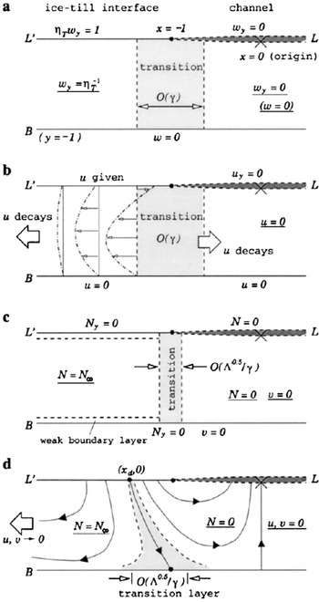
On the other hand, we have P ≫ P i just outside the channel, P = p c just inside, and thus at the margin (x = −1) itself, dP/dx is undefined. This induces a large sediment flow there into the channel. We can also approximately solve Equations (103)1 and (105) inside the channel. In −1< x < 0, sensible leading-order solutions are w = u = 0 (η T vanishes also). Thus, sediment-flow velocities at the margin must decay as we move inside the channel.
The velocity field u is therefore quite complicated: till deforms away from the neighbourhood of x = −1 both into the channel and to the far field (Fig. 11b). The sign change in u must be accompanied by a dividing streamline adjoining L′ and B (cf. section 4.3). Across the margin, an abrupt switch occurs between the leading-order solutions (for both u and w) in x < −1 and −1 < x < 0. How are these achieved? So far, our derivation has neglected x derivatives, specifically the terms γ 2 ∂(η T ux )/∂x and γ 2 ∂(η T ux )/∂x appearing in Equations (103)1 and (105). As u and w fluctuate rapidly near the margin, these terms become important and the leading-order approximations break down. Roughly speaking, this happens within a distanceFootnote * of O(γ) from the margin (corresponding to a width of the order of the till thickness). In this transition region, the discontinuities are smoothed out. We show these results schematically in Figure 11a and b. (Mathematically, the equations which describe the transition region constitute what is known as an “inner” problem. Solution of this is not attempted here.)
In summary, we expect the creep flow to be concentrated in the neighbourhood of (±1, 0), mainly due to the contact stress singularity, but also because of till viscosity reduction there as N is reduced from N
∞. Within the transition region, Equation (107)
1 shows that reduction in η
T is further enhanced by the flow itself, since (1 – a)/2a < 0, and the term
![]() will become significant. Here, the size of S helps determine the importance of ∂u/∂y as compared to ∂w/∂y (which represents τ
12) in this reduction. We consider N(x, y) next.
will become significant. Here, the size of S helps determine the importance of ∂u/∂y as compared to ∂w/∂y (which represents τ
12) in this reduction. We consider N(x, y) next.
Effective stress and permeability limits
Let us say γ = 0.1, then with the current scales we obtain

But generally this ratio can fall within an even greater range, since we have taken only nominal values for k T, [η], l and γ. (Remember Λ ∝k T/[η]−1 l 2) Specifically, Λ/γ 4 can be small or large, depending on the till composition. As we now demonstrate, the end limits of this parameter allow decoupling of the deformation and percolation problems, associated with different approximations of Equations (104).
Equations (104)1 and (104)2 describe, respectively, mass conservation and convective diffusion of N, and have the boundary conditions (i) v = 0 on B, (ii) V = 0, so that ∂N/∂y = O(γ) ≈ 0 on L′ and B, (iii) N → N ∞ as |x| → ∞, and (iv) N = 0 on L. If Λ/γ 4 ≪ 1, then they simplify to
which indicate an essentially constant density till, with the effective stress N advected (and preserved) along streamlines. Since Λ is a measure of permeability relative to deform-ability, Λ/γ 4 ≪ 1 refers to a subglacial till in which Darcy drainage is relatively inefficient. Then, pore water is simply carried along with the bulk deformation, and compaction/dilation may be neglected; this is consistent with the two results in Equation (110). For convenience, we designate such till as a “low-permeability till”, even though Equation (110) in principle applies also to a highly deformable till.
More specifically, Equation (110) is a singular approximation which breaks down near L ′ and B, and also where N changes rapidly in the x direction, because it neglects the high derivatives Nxx , Nyy and Pxx . However, boundary layers for N will be “weak”, for it is Ny (and not N) that is prescribed; see boundary condition (ii) above. Consequently, the general distribution of N(x, y) may be inferred using its boundary values and the flow structure (u, v).
The solution for u has already been described. v is determined by solving Equation (110)
1 given u. In −1 < x < 0, u = 0, we find at leading-order accuracy v = 0 (since v = 0 on B), and N = 0 (using N = 0 on L, and the fact that at leading order N is a function of x only). On the other hand, the leading-order solution in x < −1 is simply N = N
∞, since the sediment here flows toward x → −∞, and as we found earlier, N is preserved along streamlines. Thus, there is again a transition from outside the channel to the inside: N has to switch from N
∞ to zero. This takes place in a transition layer in which the neglected x derivatives (representing diffusion) become important, and N and P change rapidly. By suitable rescaling of the x coordinate in Equation (104), one can deduce that the transition region has a width of
![]() . (Thus this is inside the transition region for velocity, as
. (Thus this is inside the transition region for velocity, as
![]() . These results are shown in Figure 11c. More precisely, we speculate that this effective stress transition would take place close to the dividing streamline which we mentioned earlier, since, as discussed in section 4.3, it separates the till flow into two cells. This is sketched in Figure 11d.
. These results are shown in Figure 11c. More precisely, we speculate that this effective stress transition would take place close to the dividing streamline which we mentioned earlier, since, as discussed in section 4.3, it separates the till flow into two cells. This is sketched in Figure 11d.
Finally, we consider the “high-permeability” (or low-deformability) case Λ/γ4 ≫ 1. The corresponding approximation indicates that the till is diffusion-dominant, i.e. advection of N is negligible. Equation (104) reduces approximately to Poisson’s equation,
which is now independent of till velocities (cf. Equation (110)). Solution of this equation provides a smooth transition of width O(γ) between the leading-order solutions at the channel bed (N = 0) and far from the channel (N = N ∞). (This transition takes place near x = −1 and does not depend on the position of the dividing streamline.)
Remembering that our width scale is l, the cases Λ/γ
4 ≪ 1 and Λ/γ
4 ≫ 1, respectively, give (dimensional) transition widths of
![]() and O(d). The former width is much less than d, whereas the latter is independent of till properties. If Λ/γ
4 ∼ 1, there is full coupling between deformation and percolation, and little information may be deduced; numerical solution is then necessary.
and O(d). The former width is much less than d, whereas the latter is independent of till properties. If Λ/γ
4 ∼ 1, there is full coupling between deformation and percolation, and little information may be deduced; numerical solution is then necessary.
6. Discussions
In this paper, two models of deformation near a subglacial channel–cavity have been analyzed in an attempt to identify the potential implications of ice–till interfacial coupling for basal sliding and subglacial drainage/sediment-transport processes. Since these processes and the evolution of contact and decoupled regions are irrevocably interlinked, it has been necessary for us to make various restrictive assumptions and isolate the deformation part alone. We considered the specific scenario where the channel is aligned with the principal direction of ice flow and the till is deforming.
A non-zero positive value of effective channel pressure N c(= p i – p c) is found to have two related consequences. It induces ice and sediment to flow towards the channel–cavity, and it causes the ice–till interface to migrate via a combination of subsidence and extension just outside the channel (i.e. ±u(±l, 0) < 0, v(±l, 0) < 0). (The channel–cavity narrows as a result.) It is important to realize that our calculations are based on the pseudo-steady-flow approximation (in other words, force balance); therefore, having defined the problem geometry, our models produce “instantaneous” velocities in the ice and in the till regardless of how the problem geometry itself would then respond to other influences such as sliding and fluvial erosion. Nevertheless, our models are indicative of the general velocity dependence involved in the deformation.
The results in section 4 show that velocities in the till vary directly with the thickness of deformation, and inversely with till viscosity, so that “high” sediment flux can result for a “weak” till. To give crude examples, let us take A I ≈ 5 × 10⁻²⁴ Pa−3s−1, τ ∼ 1 bar, n = 3 for ice, so that η I = (A I τ n−l)−1 ∼ 2 × 10¹³ Pa s (≈ 6 bar a). Thus, if η I falls in the stiff end of the range 108 to 1012 Pa s, we may assume β ∼ 0.1. In this case, an order-of-magnitude estimate for the till closure velocity v T(x, 0) (i.e. in the vertical direction) and sediment flux (∼ v T × 2l) is, for d ≈ l (γ ≈ 1):

(see Fig. 9). (Here Q T is the sediment flux per unit downstream channel distance, and we have used γ = d/l to derive the bracketed term.) If we further suppose N c = 1 bar and l = 1 m, then Equation (112) gives v T ∼ 0.3 m a−1, Q T ∼ 0.6 m2 a−1, which are small indeed. However, reducing the value of η T (and hence β) can greatly increase the flow rates. Using the result in section 4.3 that v T ∝ β −2/3 for small β, a three orders of magnitude reduction of η T from 1012 to 109 Pa s would lead to v T ∼ 0.1 m d−1 and Q T ∼ 0.2 m2 d−1, for instance.
To complete the picture, we note that the deforming-till thickness may only be a fraction of the channel width. Say d = 0.1 m; then, on extrapolating similarly the results for “shallow till” (γ = 0.1, β = 1),

(see Fig. 8; note that Q T ∼ v T × 2d in this case), we obtain, for η T = 109 Pa s (i.e. β ∼ 10−4), v T ∼ 0.02 m d−1 and Q T ∼ 0.004 m2 d−1. The point is that, provided that the till viscosity is towards the low end of the spectrum, the predicted sediment flux can still be significant. This conclusion does not depend sensitively on the effective ice-viscosity value being used, since increasing η T would increase the denominators in Equations (112) and (113) but also reduce β, which has the opposite effect. For a given till viscosity, we have v T ∝ β 1/3. Hence, a factor of 103 increase in η T would reduce the velocities and fluxes by a factor of 10 only. (In addition, we may deduce from the bracketed terms in Equations (112) and (113) that for a given deforming depth d, a large channel (where γ ≪ 1) is a more efficient sediment collector than a small channel (where γ ≫ 1), if steady flow conditions were to prevail in the channel.)
Likewise, although the velocities of lateral migration of the contact margins (u(±l, 0)) are only a fraction of v T (see Figs 3 and 7–10), they may become relevant in a sliding theory that considers the basal stress distribution between contact and decoupled regions. This is particularly true if these two types of region occupy comparable areas, as may occur for a distributed system of subglacial channels or cavities. The actual migration velocities are likely to be higher than those predicted here, since marginal stress localization will soften the ice there (reduce η I), and for non-linear viscosity till, we showed also that there is further reduction of η I in the neighbourhood of the channel margins (section 5.3).
If a shallow deforming till is underlain immediately by bedrock, then subsidence of the ice–till interface may (eventually) lead to pinch-out of the till near the channel margins. Since ice–till and ice–bedrock interfaces are likely to exhibit quite different mechanical properties, this presents another mechanism whereby the nature of basal contact regions may be modified. Although the problem geometry changes continuously as the thinning process takes place, a rough estimate of the pinch-out time-scale (for η I = 1013 Pa s, η I = 109 Pa s, N c = 1 bar, l = 1 m, d = 0.1 m) based on extrapolating Equation (113) 1, is [t p ] = 20β 2/3 dη I/N c l ∼ 5d; the thinning can be quite rapid. On the other hand, if the sediment deposit was deep, a natural extension would be to incorporate a yield stress in the model, which leads to a free boundary problem. Besides being useful in verifying our assumption of constant deforming thickness, this may have interesting geomorphic consequence. The pinch-out process, together with downward migration of the yield boundary near a subglacial channel, may provide a mechanism for the formation of tunnel valleys, as first envisaged by Reference Boulton and HindmarshBoulton and Hindmarsh (1987).
The tendency for the system to increase the contact area between ice and till (and conversely, to decrease the channel area) may have implications for channelized drainage. Since our model does not consider the effect of fluvial processes on the till, it is not possible to say at present whether soft-bed channels can remain stable, and under what conditions they would do so. Conceivably, channels can persist if the timescale for coupled deformation is significantly longer than that for sediment erosion and deposition (see Reference NgNg, 2000). Even without resorting to elaborate drainage theories, however, we can see that till sediments relocated to within the channel will become susceptible to fluvial erosion. In this way, coupled deformation provides a transport mechanism which should not be neglected in sediment budget analysis.
Obviously, the foregoing inferences are somewhat limited by uncertainties in till rheology, especially by plausible values for (the range of) η I, a and b, and thus they are at best qualitative; but they do suggest that closer examination of coupled deformation is warranted. And more than anything else, our investigation points to the need for more detailed measurement of till rheology. Only then might it be possible to generate a quantitative theory that encompasses soft-bed sliding and drainage consistently.
Acknowledgements
I would like to thank R. Hindmarsh and S. Marshall for their comments on an earlier version of this paper, and N. Iverson, S. Tulaczyk and J. Walder for constructive and critical reviews. A. Fowler continues to provide great inspiration. This work is supported by a Junior Research Fellowship at St John’s College, University of Oxford.
Appendix I
(a) Combinations of C 3…C 6(λ)
Let us define
Manipulation of Equations (43), (44), (46) and (47) then leads to


(b) Formulae for the stress and velocities
The following results have been derived by applying the inverse Fourier transform in Equation (29) to the stress/velocity relations in Equations (23), (27) and (28), then substituting for Ψ, Π, Ω and Κ from Equation (33).
(i) Ice domain (y > 0)
(ii) Till domain (–γ < y < 0)
Define ch = cosh(yλ), and sh = sinh(yλ), then


Appendix II
The limit γ →∞
Given Equation (59), Equation (55) implies that Lm , n = 0 when m + n is odd, and that

when m + n is even. By applying the standard result (Reference Gradshteyn and RyzhikGradshteyn and Ryzhik, 1980, p.679)

we may further deduce that

and hence, by Equation (54), αn = 0 for n > 1, and

The result in Equation (60) now follows directly from Equations (52) and (53).


