


Introduction
Svalbard glacier mass loss has been considerable since the beginning of the 1900s (Nuth and others, Reference Nuth, Kohler, Aas, Brandt and Hagen2007; Möller and Kohler, Reference Möller and Kohler2018). Air temperature, the main driver of glacier mass balance, has risen by 2.6°C in the last century, with a rate of increase that has accelerated in the last ~50 years (Nordli and others, Reference Nordli, Przybylak, Ogilvie and Isaksen2014). Quantification of glacier melt in this period is important for understanding how glaciers have responded to prolonged warming, and to figure out how unique the recent climatic trend of the past century is, compared to previous warming events before the observational period. Inventories of glacier extents and area on Svalbard show a 13% decrease in ice cover since the end of the Little Ice Age (LIA; Martín-Moreno and others, Reference Martín-Moreno, Allende Álvarez and Hagen2017), a cold period spanning a few hundred years (Mann and others, Reference Mann2009). The end of this cold period on Svalbard featured overall glacier retreat, but the timing of this event is still unclear, as the lack of data inhibits a clear picture. However, maps and observations seem to suggest that the onset of retreat occurred sometime in the late 1800s (Liestøl, Reference Liestøl1988; Lefauconnier and Hagen, Reference Lefauconnier and Hagen1991; Svendsen and Mangerud, Reference Svendsen and Mangerud1997). Glacier surges occur more frequently on Svalbard than anywhere else in the world (Sevestre and Benn, Reference Sevestre and Benn2015). Surges are dynamic instabilities that result in dynamically driven advance and retreat phases, which complicate the relationship between climate change and the geometric response of individual glaciers (Yde and Paasche, Reference Yde and Paasche2010). The total Svalbard glacier area has nevertheless decreased by 7% over the last 30 years, indicating an accelerating retreat rate (Nuth and others, Reference Nuth2013).
While area change is an important parameter, and more readily quantifiable, changes in volume are most directly connected to the effects of climate change, and it is therefore especially valuable to estimate volume change, where possible. For Svalbard, this has recently been reconciled for 2000–2019 by combining glaciological with geodetic mass-balance data (Schuler and others, Reference Schuler2020). Other recent studies have used modern photogrammetry for calculating glacier volume change from aerial images taken on Svalbard in 1936 (Mertes and others, Reference Mertes, Gulley, Benn, Thompson and Nicholson2017; Midgley and Tonkin, Reference Midgley and Tonkin2017; Girod and others, Reference Girod, Nielsen, Couderette, Nuth and Kääb2018). In this study, photogrammetric reconstructions are performed even further back in time, to 1910 and 1911, to gain a better understanding of the timing and extent of post-LIA glacier retreat on Svalbard. Aldegondabreen is used as an example glacier, as its high temporal and spatial coverage of images gives a powerful example of what a more widespread use of archival photographs can deliver.
A number of photogrammetric surveying campaigns were carried out during the early 1900s, and the resultant photographs are now archived by the National Library of Norway. These surveys were carried out to create accurate and reliable topographic maps, which were used for research, and later, for territorial claims by Norway (Barr, Reference Barr and Isachsen2009). Surveying was initially performed mostly by theodolite, complemented by photogrammetry, but from the 1910s and onward, photographs became the predominant sources of information. This resulted in many glaciated areas being covered by tens or more photographs in the same year, and tens of thousands of photographs are now archived and available for scanning, with enough overlap to utilise modern photogrammetrical processing techniques for extracting accurate topographic data.
Study area
Aldegondabreen (77.97°N, 14.05°E) is a 2.6 km long terrestrial valley glacier in Grønfjorden on Svalbard, located 8 km from the Russian mining settlement of Barentsburg (Fig. 1). The mean annual air temperature and total annual precipitation in 1961–1990 at Barentsburg were − 6.1°C and 565 mm w.e. (water equivalent), respectively, with statistically significant positive trends for both parameters (Hanssen-Bauer and others, Reference Hanssen-Bauer2019). In the early 1900s, photographs show that Aldegondabreen was around 5 km long and terminated in the fjord, but it is today roughly half as long (Fig. 2). Today, it covers 5.7 km2, with an elevation range of 200–600 m a.s.l. Throughout its observational history, the glacier ice margin had little debris cover, making it easy to delineate changes in its length and areal extent. The glacier had an average thickness of 73 m in 1990, with temperate ice in its thicker southern half, overlain by a thick cold surface layer (Navarro and others, Reference Navarro2005). Unpublished radar data from 2017 by the University Centre in Svalbard show that the glacier still has a small temperate core, but it has drastically reduced in size. The geomorphology of the glacier's forefield suggests a more temperate regime in the past, as seen by the presence of flutes, roche moutonnées and striated clasts (Kirkebøen, Reference Kirkebøen2018). In 1864, a Swedish expedition noted extensive calving of a tidewater glacier in Grønfjorden (Dunér and others, Reference Dunér, Malmgren, Nordenskiöld and Qvennerstedt1867). Since Aldegondabreen was the only glacier terminating in the fjord, this indicates a much higher ice flux at that time. The glacier was retreating already in 1910, as evidenced by a smooth terrestrial terminus and a well-developed calving bay. The terrestrial forefield geomorphology and low-resolution soundings in the fjord by the Norwegian Mapping Authority suggests a slightly larger Neoglacial maximum than in 1910, maybe corresponding to the late 1800s LIA culmination or of a larger older extent. The characteristics of the glacier's rapid subsequent decline is interesting, as surge-indicative landforms exist in its forefield (Farnsworth and others, Reference Farnsworth, Ingólfsson, Retelle and Schomacker2016).
Study location on Svalbard (red rectangle) and the location of Longyearbyen (LYB), the main settlement on Svalbard (a). The surroundings of Aldegondabreen, showing the constructed GCPs used in the terrestrial, aerial, or both types of reconstructions (b). The locations of the used 1910/11 photographs are shown together with their orientations.

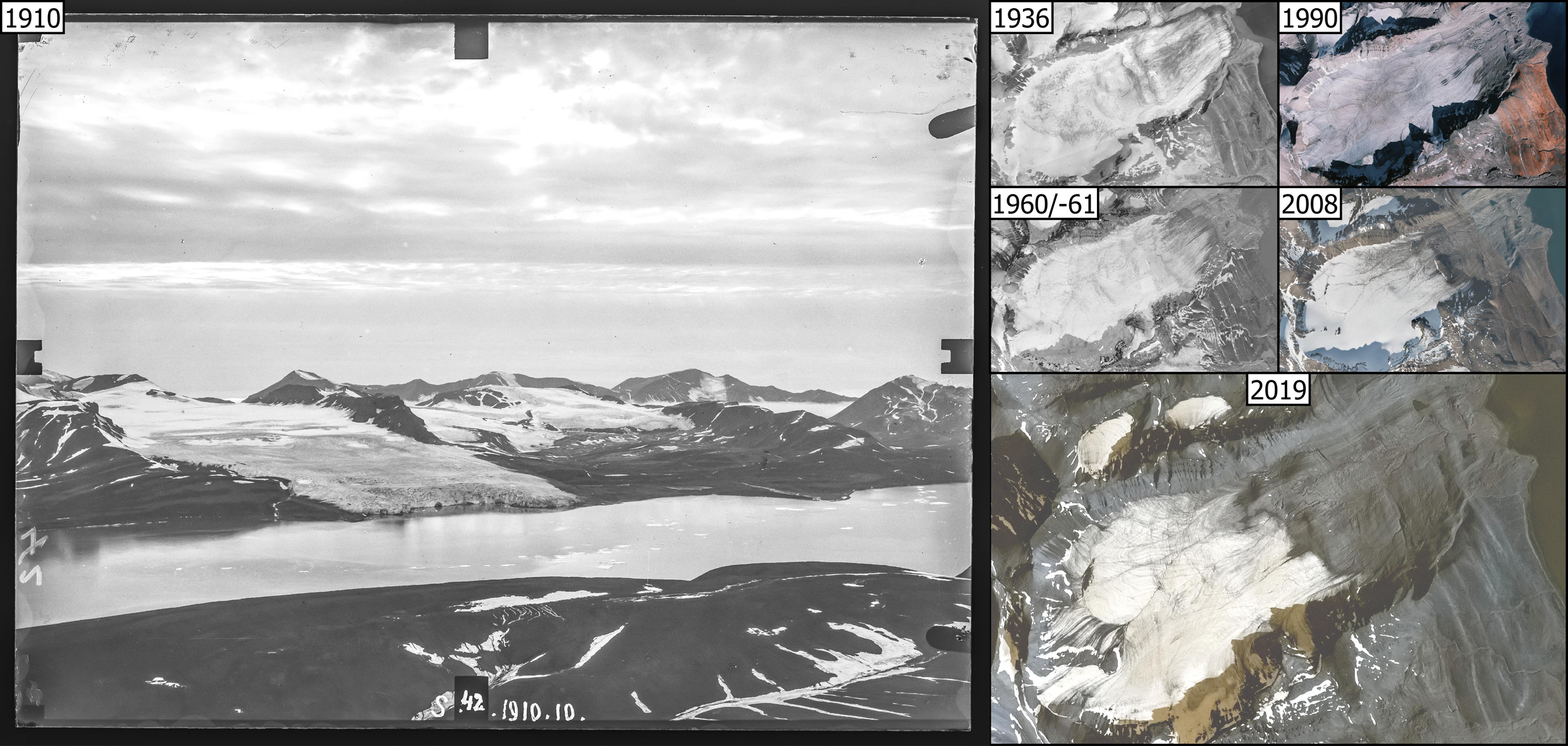
Example photograph for the 1910/11 reconstruction (left), taken from the opposite side of the fjord. The fiducial marks around the frame are used to align the photographs’ internal coordinate system. Orthomosaics (upper right) from the multiple aerial surveys performed by the NPI. A Planet satellite image (lower right) shows the 2019 state of the glacier.
Data and methods
Terrestrial photographs
A total of 17 photographs from 1910 and 1911 are known to cover Aldegondabreen (Figs 1 and 2). The 9 × 12 cm glass plate positives from 1910 and 1911 were scanned for the purpose of this study at 1600 dpi by the National Library of Norway, equating to approximately 42 megapixels for each image. They were preprocessed in Adobe Photoshop CC 2019 by applying noise reduction, sharpening and contrast enhancement filters using the same settings for each image.
Aerial photographs
Late-summer photographs from aerial surveys are available for Aldegondabreen in 1936, 1956, 1960, 1961, 1969, 1990 and 2008. The 1936 survey consists of images taken at an oblique (~ 30° from horizontal) angle, and the images in 1956 and later were taken vertically. The 1960 and 1961 surveys each covered only parts of Aldegondabreen, but taken together provide full coverage. The subsequent reconstruction was assigned a single time stamp since the photographs were obtained with only a year between them (Fig. 2). Variable snow cover was assumed to play a larger role than one year's variation in ice elevation, so this was considered a safe approach. The 2008 survey is already processed by the NPI, yielding a well georeferenced orthomosaic and a 5 m Digital Elevation Model (DEM; www.npolar.no), which was used here as a reference data set.
Other data
An ArcticDEM strip (scene id: WV02_20160702_1030010) derived from 2016 WorldView satellite imagery (Porter and others, Reference Porter2018) was used for modern elevation change, and was co-registered using the vertical difference of stable terrain (c.f. Rodrıguez and others, Reference Rodrıguez, Morris and Belz2006; Berthier and others, Reference Berthier2007; Howat and others, Reference Howat, Smith, Joughin and Scambos2008). In addition, a Planet satellite scene from 2019 was used for areal extent change (scene id: 20190803_062019_1_0f2b; Planet Team, 2019). To put the elevation change of Aldegondabreen in context, its mean thickness of 73 m in 1990 determined by Navarro and others (Reference Navarro2005) was used to determine the current and past ice thickness. These depth data are available through the Glacier Thickness Database 3.0 (GlaThiDa Consortium, 2019), and were used for visualisation of the glacier's profile. No error measure is given for the depth estimate, and is therefore only treated as a potential qualitative source of error.
Photogrammetry
Terrestrial and aerial surveys were processed in the photogrammetric suite Agisoft Metashape 1.5.0. The aerial photographs could be processed in a standard photogrammetric workflow and were processed using similar processing parameters (Table 1). The software employs structure-from-motion (SfM) photogrammetry, which enables the estimation of relative positions of photographs, as well as one or multiple camera models to correctly account for geometric distortions, yielding topographic information on the imaged terrain or object (Koenderink and van Doorn, Reference Koenderink and van Doorn1991; Snavely and others, Reference Snavely, Seitz and Szeliski2008; Westoby and others, Reference Westoby, Brasington, Glasser, Hambrey and Reynolds2012). This allows almost any image to be used, as long as the internal coordinate systems of the images are consistent, which is handled with fiducial marks in scanned imagery (Fig. 2). Similar studies of archival aerial images give examples of this potential (Koblet and others, Reference Koblet2010; Mölg and Bolch, Reference Mölg and Bolch2017; Vargo and others, Reference Vargo2017; Girod and others, Reference Girod, Nielsen, Couderette, Nuth and Kääb2018). The flexibility of Metashape allows both the aerial and terrestrial surveys to conveniently be done in the same framework, but limitations of this approach with the terrestrial photographs are discussed later.
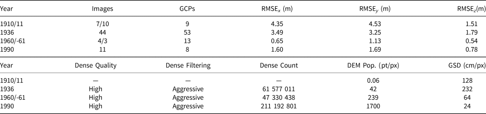
Properties of the photogrammetric reconstructions. The dense quality refers to the resolution of the MVS reconstruction in Metashape (‘high’ means that depth maps are generated at half the image resolution), dense filtering is the proprietary depth map filtering setting, and dense count refers to the resultant point cloud count. The 1910/11 reconstruction was based on manual triangulation, giving it a much lower resultant 20 × 20 m DEM population. The ground sampling distance (GSD) is the default orthomosaic resolution reported by Metashape.
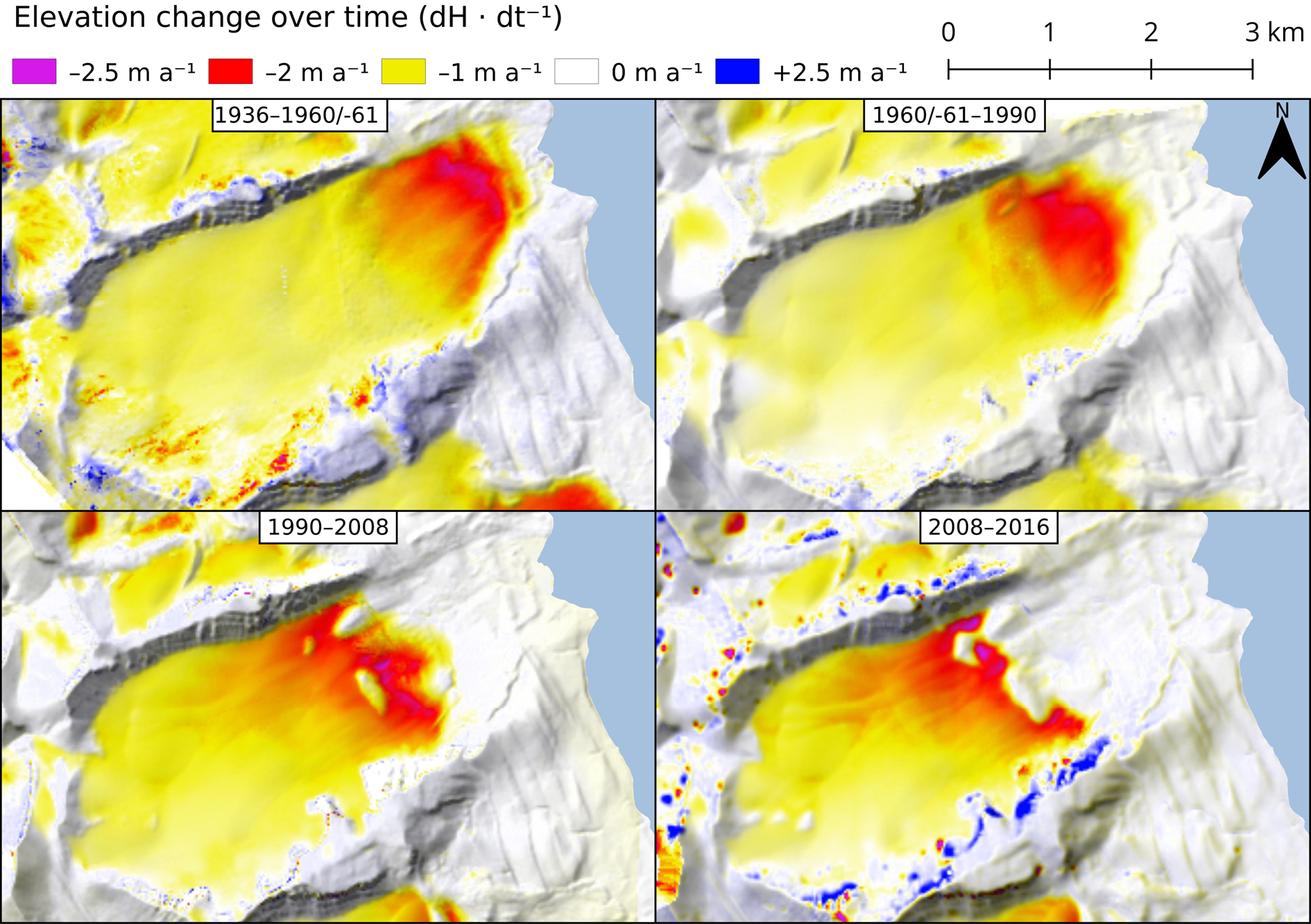
Point clouds, which are used to create Digital Elevation Models (DEMs), and orthomosaics, are the products of the photogrammetric processing in Metashape, and the DEMs and orthomosaics were analysed in QGIS 3.8.0 to determine the changes in size of Aldegondabreen. DEM gridding was performed in CloudCompare v.2.10.2 instead of Metashape, to enable equal gridding of 20 × 20 m DEMs for each survey. This simplified the subsequent analyses as the DEMs were exactly aligned, and no resampling (with possible inherent error) was needed to compare them. Elevation change was calculated by subtracting each consecutive DEM, and interpolating gaps in the DEM difference (dDEM) products using linear spatial interpolation (Fig. 3). Smaller gaps in the DEMs arose in the low-detail zones created by shadows, but this usually has a negligible impact on the overall result (McNabb and others, Reference McNabb, Nuth, Kääb and Girod2019). The dDEMs were cropped to the largest glacier extent in respective DEM pairs, and the mean thickness difference was multiplied by this area to yield the volume change. Elevation profiles, area and length variation (based on ten equally spaced parallel transects), calculated from the data, further helped to understand the glacier's changes.
Elevation change between the aerial image reconstructions. The background hillshade is from the latter year in the comparisons. Negative elevation change retained its order of magnitude (ca. –2 m/a), in spite of the glacier retreating to higher elevation.
Ground control points (GCPs) are normally needed for photogrammetric reconstructions, to georeference the images and allow comparisons between surveys (Smith and others, Reference Smith, Carrivick and Quincey2016). This is preferably done by collecting them in the field with a differential GNSS receiver (e.g. Rosnell and Honkavaara, Reference Rosnell and Honkavaara2012; James and others, Reference James, Robson and Smith2017). If this is not possible, a reference data set can be used to derive 3D-coordinates of boulders and other features in terrain assumed to be stable that can be seen in the historic images, which is advantageous with respect to quantity over quality, when compared to the field-based approach (e.g. Hong and others, Reference Hong, Jung and Won2006; Mertes and others, Reference Mertes, Gulley, Benn, Thompson and Nicholson2017; Girod and others, Reference Girod, Nielsen, Couderette, Nuth and Kääb2018). The dominant flora in the study area are Northern Woodrush and a multitude of mosses, which grow from less than one to a few decimetres in height (Elvebakk and Prestrud, Reference Elvebakk and Prestrud1996). Vegetation cover in the study area was therefore a good indicator of unchanging ground, and features were consequently sought with its presence. The 2008 orthomosaic and DEM, which together served as a reference model, was used to extract 65 unique GCPs spread around the study area (Fig. 1). The number of GCPs used for each survey, and their respective errors, are shown in Table 1.
Terrestrial photogrammetry
The 1910 and 1911 photographs of Aldegondabreen have a high degree of overlap, with up to 13 photographs covering one feature. In spite of this fact, manual input was needed to align them all, requiring considerable extra time and effort, and 102 manual tie points were added. Each manual tie point was defined in between 2 and 13 photographs (5 on average), with a mean pixel error of 2.95 px (equivalent to around 4 m in projected coordinates). The automatic alignment in Metashape gave poor results, with 2 801 tie points being identified in only 3 out of the 17 total photographs. This meant that each photograph could be aligned, but with a higher uncertainty than what would otherwise be possible. Attempts at dense reconstructions using the Multi-View Stereo (MVS) algorithm in Metashape were also too noisy to use, so only the manually triangulated points were considered reliable.
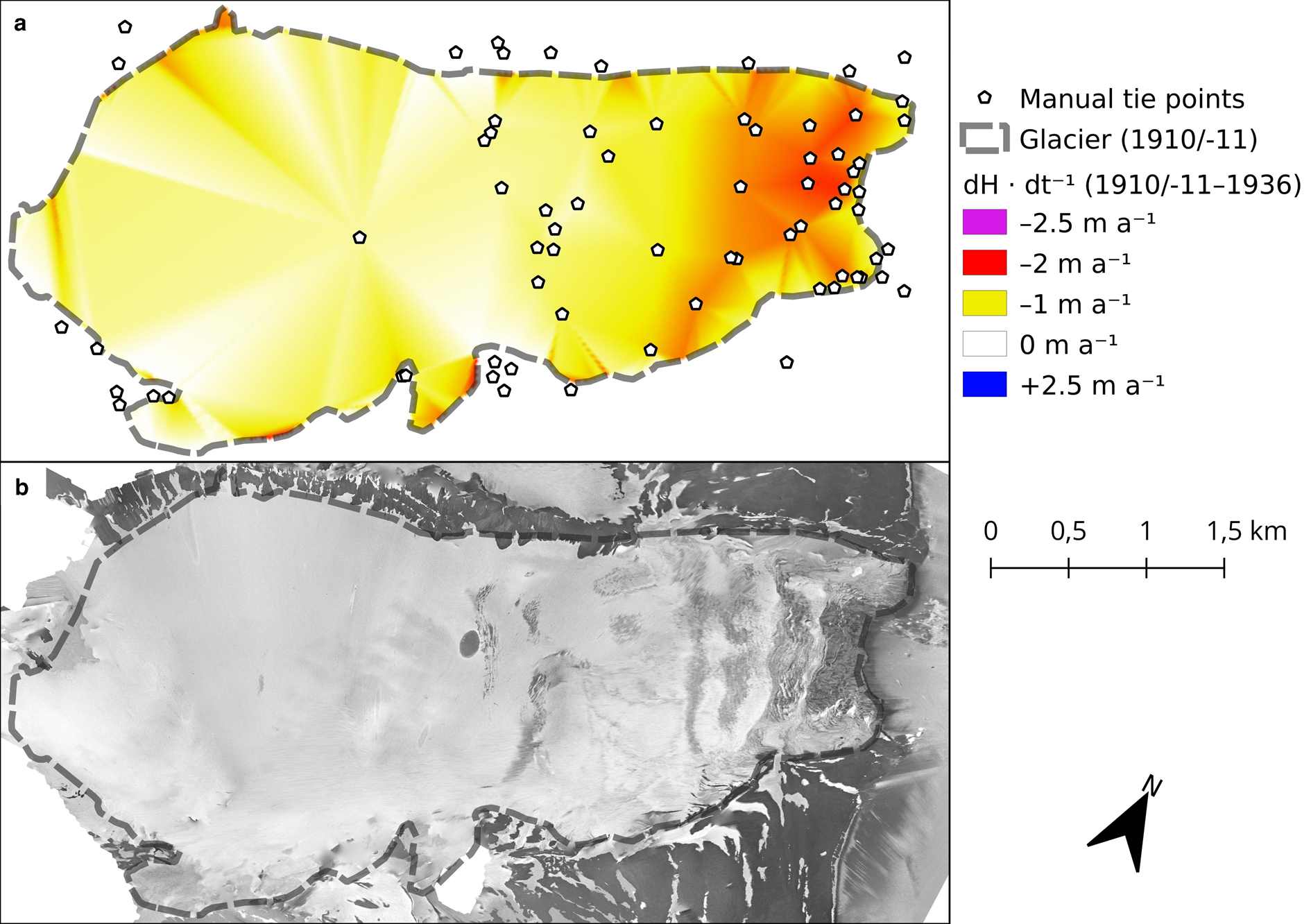
Due to the sparse nature of the viable topographic data, a more advanced interpolation methodology was needed to feasibly interpolate a 1910/11 surface DEM. Due to low detail in the snowy upper parts of the glacier, only one point was successfully triangulated using three images on the upper half of the glacier. The edge of the glacier was however easy to identify through the photographs and was therefore used as an additional indicator of the glacier's past size. The elevations of the 1910/11 boundary line on the rock wall was compared to the elevations of the 1936 boundary, and was used as additional point values, together with the traditionally triangulated points. The 1910/11 outline was made by projecting the outline drawn in each photograph onto the 2008 DEM, which was assumed to accurately represent the mountain side in 1910/11, to yield the 3D position of the boundary. Finally, elevation changes between 1910/11 and 1936 (Fig. 4) were interpolated, which is a statistically more accurate method than first interpolating and then differencing elevations values (McNabb and others, Reference McNabb, Nuth, Kääb and Girod2019). A 1910/11 DEM was constructed by subtracting the 1910/11–1936 elevation differences (dDEM) from the 1936 DEM. The surface thus inherits the general shape of the glacier in 1936, which is not unrealistic, but remains an untestable assumption of the methodology. However, significant changes in surface morphology usually do not occur in the absence of any surge-type behaviour. Since there is only a faint geomorphological inference for past surging (Farnsworth and others, Reference Farnsworth, Ingólfsson, Retelle and Schomacker2016), and no indication of a surge in the study period, assuming a constant shape seemed reasonable.
Elevation change between the terrestrial 1910/11 and aerial 1936 reconstruction, and the location of the constituent manual tie points, used together with the boundary difference to interpolate the dDEM (a). Orthomosaic from the 1910/11 reconstruction, draped on the resultant DEM (b).
Error assessment
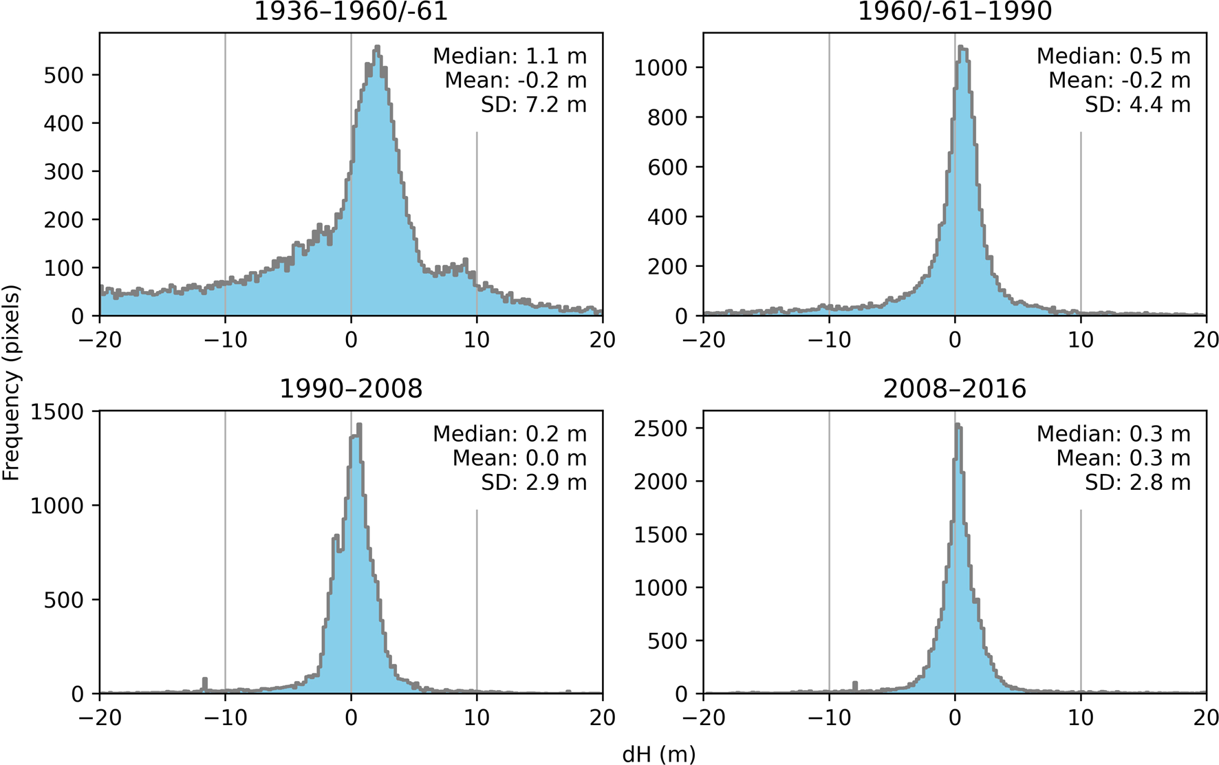
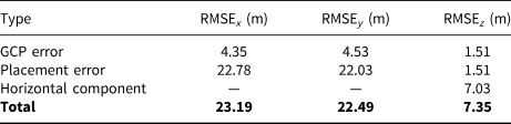
Elevation errors in photogrammetric reconstructions are typically characterised by the Root Mean Square (RMS) of the elevation differences between the estimated GCP positions and their corresponding reference position (e.g. Kääb, Reference Kääb2005; Koblet and others, Reference Koblet2010; Mertes and others, Reference Mertes, Gulley, Benn, Thompson and Nicholson2017; McNabb and others, Reference McNabb, Nuth, Kääb and Girod2019). This was used for the aerial image reconstructions, but additional error sources were expected to play a role in the terrestrial image reconstruction since the process was not performed in a well-established workflow. In addition to the GCP uncertainty, elevation data were extracted by manual triangulation, which produces fewer points and is therefore more prone to erroneous outliers affecting the final result. The triangulation uncertainty was assessed by evaluating the location variance when each available combination of image pairs was used to define it separately (c.f. Holmlund and Holmlund, Reference Holmlund and Holmlund2019): For each manual tie point, every unique combination of image pairs used to define it were tested, and the resulting position of the point was noted. The RMS of the deviation from the mean of each point was thus used to estimate the uncertainty. While only the vertical components of errors are traditionally used for vertical difference error, the horizontal uncertainty was assumed large enough to require consideration. The mean slope of the 1910/11 DEM was 12°, so the total horizontal error was multiplied by sin(12°) to approximate the vertical effect of the horizontal component, adding to the total vertical error of the reconstruction (Table 2). Since the 2016 ArcticDEM lacked an associated alignment error, the RMS of the residual error after registration to the 2008 DEM was used instead. Finally, the elevation differences between the aerial and satellite reconstructions on stable terrain (assumed from extensive vegetation) were calculated, to provide an additional error measure (Fig. 5). These differences were normally distributed around medians with lower magnitudes than the calculated vertical alignment root mean square errors (RMSE; Table 1), thus supporting that the initial error assessment is representative.
The median, mean and standard distribution (SD) of the offsets of stable terrain in the aerial and satellite data comparisons (see Fig. 3). The y-axes represent the number of 20 × 20 m pixels that occur in each bin (bin-width = 0.2 m).
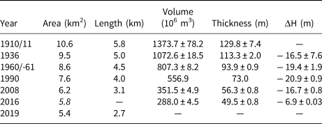
Variations in area, length, volume, thickness and elevation change for each year interval. The 2016 area was calculated by linear interpolation between the 2008 and 2019 values, to allow multiplication with the concurrent thickness
Results
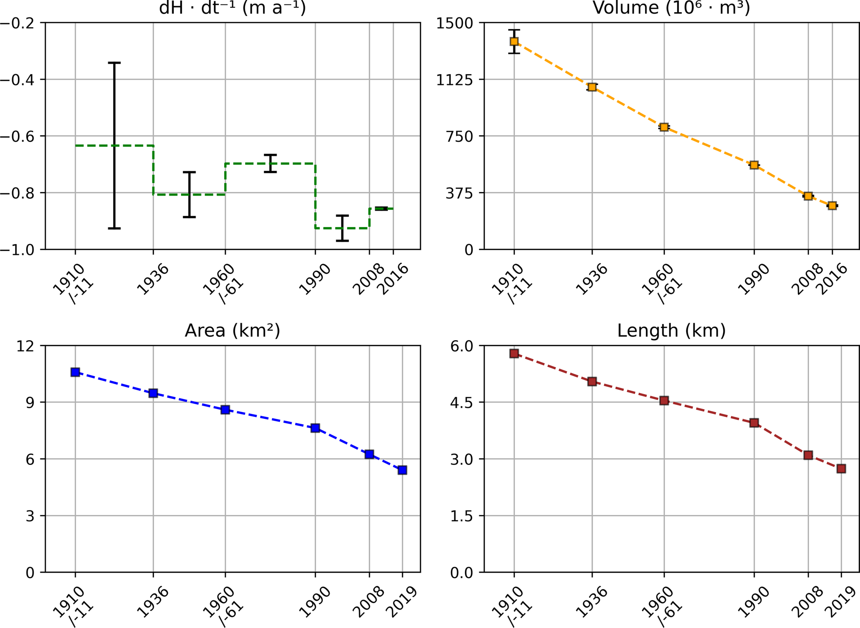
The reconstructions of Aldegondabreen show a $79\percnt \pm 6\percnt$ volume loss between 1910/11 and 2016 (Table 3). During the same time, it was roughly halved in area and length (Fig. 6). There was no clear change in the rate of volume loss between the studied years ($-10.1 \pm 1.6 \cdot 10^6\ {\rm m}^3\, {\rm a}^{-1}$
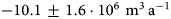 ), with a linear Pearson correlation coefficient of 0.9986, suggesting that the entire 1900s featured considerable ice loss. However, there is an accelerating rate of elevation loss, similar to other parts of Svalbard (Kohler and others, Reference Kohler2007; James and others, Reference James2012; Nuth and others, Reference Nuth, Schuler, Kohler, Altena and Hagen2012; Małecki, Reference Małecki2013, Reference Małecki2016). Since ~1990, a similar acceleration in area and length reduction is seen, although data with a higher temporal resolution would be preferable to say this with certainty (Fig. 7).
The variation in areal extent of Aldegondabreen since 1910/11, compared to its approximate Neoglacial maximum (a). The topographic profile is shown in Fig. 8. Equally spaced lines along the approximate glacier centreline were used to calculate the glacier's changing length (b).

Variation in size of Aldegondabreen, with the corresponding error in elevation change and volume (c.f. Table 3). The yearly elevation change (dH · dt −1) seems to indicate an acceleration, unlike the rate of volume loss. The rates of reduction in length and areal extent may have accelerated since 1990, but data with higher temporal resolution would be preferable to say this with certainty.
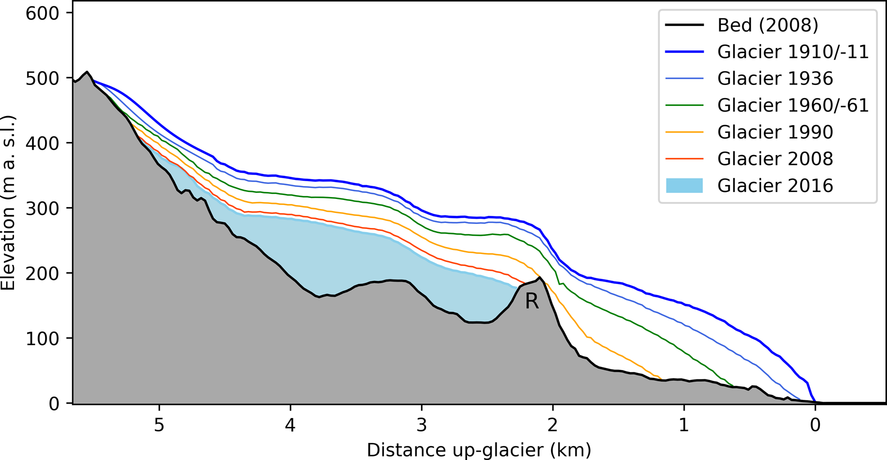
Elevation profile of Aldegondabreen, and its geometric changes over time. The main bedrock riegel (R) is clearly reflected in the reconstructed ice surfaces.
Aldegondabreen lost ice even in its uppermost elevations, unlike some higher elevation Svalbard glaciers, where remote sensing and modelling suggests that increased melt is counteracted by increased precipitation (and thus accumulation), yielding positive thickness change in the upper parts (Moholdt and others, Reference Moholdt, Nuth, Hagen and Kohler2010; van Pelt and others, Reference van Pelt2019). Additionally, surge-type glaciers often tend to show a thickening in the upper parts during quiescence, even as the overall mass balance may be negative (Nuttall and others, Reference Nuttall, Hagen and Dowdeswell1997; Melvold and Hagen, Reference Melvold and Hagen1998; Benn and others, Reference Benn2019; Nuth and others, Reference Nuth2019). This does not seem to be the case for Aldegondabreen; there is no clear indication of past surging, and its accumulation area is too low to take advantage of any positive mass change from the ongoing precipitation increase. Aldegondabreen, and other low-elevation glaciers like it, could only have remained unchanged in a much colder or wetter climate than that of the 1900s. Linear extrapolation of the volume loss suggests that Aldegondabreen will be almost non-existent by the 2040s.
Discussion
Few glacier reconstructions predating the 1936 aerial photography campaign have been performed on Svalbard. Topographic maps older than 1936 have been used to draw profiles or to calculate glacier extent (Liestøl, Reference Liestøl1969; Nuttall and others, Reference Nuttall, Hagen and Dowdeswell1997; Pälli and others, Reference Pälli, Moore, Jania and Glowacki2003; Flink and others, Reference Flink2015, Reference Flink, Hill, Noormets and Kirchner2018). However, the associated errors are large and sometimes difficult to quantify, although the workflow suggested by Weber and others (Reference Weber, Andreassen, Boston, Lovell and Kvarteig2020) may help in standardising these errors. Since no similar historic terrestrial reconstructions have been done on Svalbard before 1936, the results of this study lack a good comparison. It is however evident that this approach is more reliable than those using topographic maps, which often have large systematic errors that are difficult to quantify without a reference dataset (Lightfoot and Butler, Reference Lightfoot and Butler1987; Fisher and Tate, Reference Fisher and Tate2006; Surazakov and Aizen, Reference Surazakov and Aizen2006). Digitally reprocessing these archival photographs may mark a significant milestone in our understanding of the effects of climate change and glacier dynamics just at the end of the LIA.
The underlying topography of Aldegondabreen is complex, due to heavy tectonisation of the geological units in its surrounding (Dallmann, Reference Dallmann2007). This may impact the glacier's dynamics, and thus alter its reaction to climate change. A major bedrock riegel is present beneath the past surface of Aldegondabreen which most likely disturbed the ice flow (Fig 8). Large riegels can severely affect flow direction and speed, and will thus control how a glacier reacts to increased melt (Hooke, Reference Hooke1991; Hanson and others, Reference Hanson, Hooke and Grace1998; Holmlund and Holmlund, Reference Holmlund and Holmlund2019). In addition, ice buildup above such topographic controls, which act as barriers, can possibly lead to surges (Flowers and others, Reference Flowers, Roux, Pimentel and Schoof2011; Lovell and others, Reference Lovell, Carr and Stokes2018). Melt rates and dynamics of Aldegondabreen could have been affected by factors such as these in the past, but the results of this study offer no proof, neither for nor against this possibility. The best course of action is to reconstruct more glaciers in the same historic time-frame, which would help to determine whether the response of Aldegondabreen to 1900s century climate change is regionally representative.
This reconstruction shows that invaluable information can be extracted from such archival terrestrial photographs. However, the automatic processes of Agisoft Metashape were not suitable for more extensive reconstructions, due to the need for time-consuming manual processing, and yielded more sparsely distributed data than might normally be expected. Analyses of similar archival photographs might benefit from more comprehensive image preprocessing and from algorithms that are better suited for feature extraction from archival imagery. Image preprocessing can be automated by scoring the workflow using the amount or the quality of extracted features in an image, where more or better features indicate a better preprocessing workflow, and this approach is encouraged to develop further. Next, other feature detection algorithms than the built-in Scale Invariant Feature Transform (SIFT) implementation in Metashape may be better at extracting features from archival imagery. The potential of the current approach is nevertheless intriguing, as many other areas on Svalbard are covered by similar photographic material. Elevation change data from the early 1900s would yield complementary data to aid and augment the mass-balance model reconstructions afforded by century-scale meteorological reanalysis products (e.g. Möller and Kohler, Reference Möller and Kohler2018).
Conclusion
The aim of the study was to evaluate the possibility of using historic archival photographs on Svalbard to reconstruct the past shape and size of its glaciers. Photogrammetric analyses of oblique terrestrial photographs taken in 1910 and 1911 of Aldegondabreen, combined with data from aerial imagery and satellite data, yielded promising results, and point to the possibility of a more widespread application, since there are abundant photographs from the early 1900s in other regions of Svalbard. The reconstruction showed that there was a $79\percnt \pm 6\percnt$ reduction in volume, from $1373.7 \pm 78.2 \cdot 10^6\ {\rm m}^3$
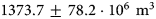 in 1910/11 to $288 \pm 4.5 \cdot 10^6\ {\rm m}^3$
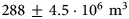 in 2016, together with an approximate halving in length and areal extent. The rate of volume change from 1910/11 to 2016 was largely constant, suggesting that the climate throughout the 1900s was unfavourable for the glacier. Over the same period, however, there was an acceleration in the rate of elevation change, most likely due to the concurrently warming air temperatures. A linear rate of volume change may be explained by an adapting geometry occurring synchronously with the temperature rise. Extrapolation of the rate of volume change suggests that the glacier may be almost non-existent within 30 years. Similar photographic material from the early 1900s exists in many other regions of Svalbard, and the potential of its use is shown here. Use of these in a larger extent with an improved processing workflow may yield invaluable information on the history, and future prospects, of glaciers that may not exist in the near future.
Acknowledgments
We thank Lena Håkansson for help with image acquisition and for supervision of the project. The Norwegian National Library and Norwegian Polar Institute are also acknowledged for their kind support in finding the historic images. We also thank Andrew Hodson, Anna Bøgh, Anna Schytt and Per Holmlund, as well as two anonymous reviewers, Jack Kohler and Emily Geyman for helpful contributions to the manuscript.


 Open access