


1. Introduction
The scale effects, predicted by the first generation of the R&D-based endogenous growth models (Romer, Reference Romer1990b; Aghion and Howitt, Reference Aghion and Howitt1992), posit a proportional relationship of growth rates of knowledge (technology) and real per capita GDP to the scale of research and development (R&D) activity. However, the lack of empirical support for scale effects across developed countries is established as a stylized fact. Jones (Reference Jones1995b) eloquently summarizes it by stating that the increasing trend of either R&D labor or real R&D expenditure bears no relation to TFP (total factor productivity) growth.Footnote 1
The theoretical and empirical conundrum of scale effects led theorists to develop two classes of second-generation R&D-based endogenous growth models: (i) semi-endogenous growth models (e.g., Jones, Reference Jones1995a; Kortum, Reference Kortum1997; Segerstrom, Reference Segerstrom1998), and (ii) fully-endogenous “Schumpeterian” growth models (henceforth Schumpeterian; e.g., Young, Reference Young1998; Dinopoulos and Thompson, Reference Dinopoulos and Thompson1998; Howitt, Reference Howitt1999). In semi-endogenous growth models, scale effects are primarily supply-side effects, while in fully-endogenous growth models, scale effects can arise from both the supply side and the demand side. These two classes of growth models eliminate scale effects through different mechanisms. Semi-endogenous models assume decreasing returns to knowledge stock, which weakens scale effects as the economy advances and accumulates knowledge. Fully endogenous growth models maintain constant returns to aggregate R&D, but they offset scale effects through two main mechanisms. First, R&D at the firm level faces diminishing returns, meaning that adding more researchers to a single firm does not lead to a proportional increase in technological progress, thereby weakening the direct link between population growth and innovation. In other words, each firm undertakes its own R&D instead of contributing to a shared knowledge pool, which would otherwise scale proportionally with population growth. Second, as population grows, the number of firms and product varieties expand, maintaining a competitive market where demand per firm does not systematically increase with population size. As more firms enter, competition increases, preventing any one firm from enjoying higher per-product demand or excess profitability, which, in turn, removes the incentive for population-driven R&D growth. Following these theoretical advances—namely, the advent of second-generation growth models—empirical scrutiny of scale effects has taken a back seat. The empirical literature has mainly concentrated on developed economies, comparing the two types of second-generation R&D-based growth models by testing either technology production functions or the models’ predictions.Footnote 2
We aim to contribute to the literature both empirically and theoretically. Empirically, we obtain valid estimates of scale parameters by appropriately measuring R&D scale and employing a suitable regression specification and estimator that address issues of unbalanced regression and potential spurious parameter estimates. Our novel empirical approach uncovers significant R&D scale effects in emerging countries, but finds them absent (i.e., insignificant) in OECD countries. Theoretically, in light of the markedly different results between the developed and emerging country panels, we propose an endogenous growth model that incorporates R&D labor and capital in a distinct manner. We then analyze the dynamics of scale effects, offering a theoretical framework that reconciles our empirical findings.
To provide context, most existing empirical assessments of scale effects use either labor input ( $Z$
) in the R&D sector or total R&D expenditure (
$Z$
) in the R&D sector or total R&D expenditure ( $R$
) as proxies for the scale of R&D. These studies typically compare the time-series properties of these proxies with the growth rates of technology (TFP) and/or per capita real GDP (e.g., Jones, Reference Jones1995a), analyzing the trends between variables measured in levels versus those measured in growth rates. Variables measured in growth rates are unequivocally stationary,
$R$
) as proxies for the scale of R&D. These studies typically compare the time-series properties of these proxies with the growth rates of technology (TFP) and/or per capita real GDP (e.g., Jones, Reference Jones1995a), analyzing the trends between variables measured in levels versus those measured in growth rates. Variables measured in growth rates are unequivocally stationary, $I(0)$
, while those measured in levels are non-stationary,
$I(0)$
, while those measured in levels are non-stationary, $I(1)$
, (see Section 2). As a result, they exhibit very different data patterns (trends), which led Jones (Reference Jones1995a) to conclude that scale effects are “counterfactual.” Although these data patterns are insightful, they still leave room for valid estimation and testing of scale parameters.
$I(1)$
, (see Section 2). As a result, they exhibit very different data patterns (trends), which led Jones (Reference Jones1995a) to conclude that scale effects are “counterfactual.” Although these data patterns are insightful, they still leave room for valid estimation and testing of scale parameters.
The scale of R&D activities encompasses two key components: the labor employed ( $Z$
) and the real capital expenditure incurred (
$Z$
) and the real capital expenditure incurred ( $E$
) in the R&D sector. A focus on
$E$
) in the R&D sector. A focus on $Z$
alone, as the scale variable, suffers from the problem of omitting a relevant variable (measure of R&D scale), namely,
$Z$
alone, as the scale variable, suffers from the problem of omitting a relevant variable (measure of R&D scale), namely, $E$
, and vice versa. The use of
$E$
, and vice versa. The use of $R$
as the scale measure captures both R&D labor and capital expenditures as a single aggregate measure, however, the downsides of employing the aggregate measure are (i) it does not allow for the potentially different effects (roles) of
$R$
as the scale measure captures both R&D labor and capital expenditures as a single aggregate measure, however, the downsides of employing the aggregate measure are (i) it does not allow for the potentially different effects (roles) of $Z$
and
$Z$
and $E$
—as two distinct components of the scale of R&D—on the growth rates of per capita real GDP and/or technology (TFP), and (ii) any attempt to estimate the scale parameters in a bivariate setting—by employing either
$E$
—as two distinct components of the scale of R&D—on the growth rates of per capita real GDP and/or technology (TFP), and (ii) any attempt to estimate the scale parameters in a bivariate setting—by employing either $R$
or
$R$
or $Z$
as the scale measure—is likely to suffer from the problem of unbalanced regression (non-standard distribution) and spurious parameter estimates. This is because the theory of scale effects associates
$Z$
as the scale measure—is likely to suffer from the problem of unbalanced regression (non-standard distribution) and spurious parameter estimates. This is because the theory of scale effects associates $I(0)$
dependent variables measured in growth rates with
$I(0)$
dependent variables measured in growth rates with $I(1)$
covariates measured in levels (scales of R&D), which gives rise to the problem of an unbalanced regression (relevant tests in Section 2). To our knowledge, this issue has not been formally addressed while testing the scale effects. We address this issue by incorporating both
$I(1)$
covariates measured in levels (scales of R&D), which gives rise to the problem of an unbalanced regression (relevant tests in Section 2). To our knowledge, this issue has not been formally addressed while testing the scale effects. We address this issue by incorporating both $Z$
and
$Z$
and $E$
as covariates in estimating the scale effects. Our trivariate approach not only captures the scale of R&D appropriately and distinctly but also resolves the issue of unbalanced regression and provides valid estimates of scale parameters, so long as the two scale variables (covariates) are mutually cointegrated, and this is what we find. Thus, our estimates of the scale effects are based on a more realistic measure of the scales of R&D than has been utilized hitherto, and on an estimation strategy that addresses the issue of non-standard distribution.
$E$
as covariates in estimating the scale effects. Our trivariate approach not only captures the scale of R&D appropriately and distinctly but also resolves the issue of unbalanced regression and provides valid estimates of scale parameters, so long as the two scale variables (covariates) are mutually cointegrated, and this is what we find. Thus, our estimates of the scale effects are based on a more realistic measure of the scales of R&D than has been utilized hitherto, and on an estimation strategy that addresses the issue of non-standard distribution.
We conduct separate but parallel estimates of the scale effects across developed (DE) and emerging (EME) country panels. The DE panel includes 19 OECD countries from 1960 to 2016, while the EME panel comprises 26 emerging economies from 1988 to 2016. Over the last three decades or so, EME countries have made significant headway in their R&D activities. Both the scales of R&D and of patenting activities have gone up significantly across EME countries, and, as is well known, they have also outperformed DE countries in terms of growth rates (see Luintel and Khan, Reference Luintel and Khan2017). Nonetheless, there is little doubt that EME countries are in growth transitions and are yet to mature. In this context, a parallel scrutiny of scale effects across DE and EME countries would be interesting from the perspectives of both the first- and the second-generation growth models. This is because if DE countries operate close to their long-run equilibrium, as is widely concurred, and if scale effects are indeed the phenomena associated with growth transitions, then one would expect to find evidence of scale effects across EME countries but not across DE countries. This is exactly what we find, which underpins both the first- and the second-generation of growth models. Our results from the DE panel are consistent with the core findings in the literature that scale effects are missing in these economies as they operate close to their long-run equilibrium. Likewise, the significance of scale effects across EME economies is also consistent with the view that these countries are in growth transitions.
Theoretically, we propose a semi-endogenous growth model that explains why scale effects are present during economic transition but disappear as economies approach their long-run equilibrium. To the best of our knowledge, no formal analysis has examined the dynamics of scale effects in an endogenous growth framework that treats R&D labor and R&D capital as distinct inputs in the production function, each serving different roles in the innovation process. Our model draws from Acemoglu (Reference Acemoglu1998) and is augmented by Jones’ (Reference Jones1995a) technology production function.Footnote 3
The frontier innovation that underpins scientific progress and contributes to the enhancement of final goods production is driven by R&D activity within a perfectly competitive research sector. This sector employs scientists and engineers—i.e., R&D labor—who initiate the discovery of new innovations. When a research firm innovates, it patents its discovery and becomes a monopolist of the new technology. Then, the monopolist translates/improves the new technology into a tangible form by embedding it in a device for a profit using R&D capital.Footnote 4 In our theoretical model, we treat R&D labor as the primary input driving breakthroughs in fundamental knowledge, which aligns with much of the existing literature (e.g., Romer, Reference Romer1990b; Jones, Reference Jones1995b; Ha and Howitt, Reference Ha and Howitt2007; Luintel and Khan, Reference Luintel and Khan2009). We model R&D capital as the key input for transforming basic innovations (knowledge) into tangible, device-embedded technologies—an approach consistent with recent findings by Growiec et al. (Reference Growiec, McAdam and Mućk2023), who emphasize the critical role of R&D capital in fostering innovation and potentially reversing the decline in U.S. “ideas TFP”.Footnote 5 Our theoretical construct seeks to capture the subtle differences between basic innovations and their subsequent progression into applied and experimental innovations, without explicitly modeling this transition. Research firms without the patent can conduct research in enhancing the technology and sell the outcome of their research to the firm possessing the patent.Footnote 6
We show that scale effects are a function of an economy’s position along its path to long-run equilibrium, and that they are non-monotonically related to the shares of new technologies, which are proportional to the growth rate of technology. We characterize developed economies as those having relatively small shares of new technologies due to their large accumulated knowledge stocks (the denominator of the share). Emerging economies, on the other hand, are characterized as having relatively large shares of new technologies due to their small accumulated knowledge stocks. Small shares of new technologies across DE countries imply small scale effects, whereas large shares across EME countries imply large scale effects, unless the latter are at the very early stage of development with little or no accumulated R&D capital stock. This characteristic is a fundamental aspect of semi-endogenous growth models, in which economies experience diminishing marginal returns to innovation capacity. As a result, scale effects diminish as the level of accumulated technology rises, aligning with the notion that innovation capacity becomes progressively less sensitive to additional technological accumulation over time.
Our model further shows that when the economy converges to its balanced growth path (BGP), the rate of economic growth is driven by the growth rates of aggregate employment and technological innovations. EME countries, being at a further distance from their BGP relative to DE economies, take longer to converge. We empirically evaluate the model’s long-run growth predictions by approximating technological innovations using the flow of patent filings—a widely used measure in the literature—and find that the results are largely consistent with the model’s predictions.
The rest of the paper is organized as follows. Section 2 presents empirical estimates of scale effects, Section 3 presents the endogenous growth model, and Section 4 tests the long-run predictions of the model. Section 5 concludes.
2. Estimates of scale effects
In this section, we discuss our sample and data, lay out our econometric model and estimation method, and report the parallel results of scale effects obtained from DE and EME country panels. We have an unbalanced panel of DE countries, which consists of 19 OECD countries with data on almost all relevant variables spanning the period 1965–2016. The exceptions are (i) the data on TFP which cover the period of 1965–2014, and (ii) the employment data for Austria and Denmark which span 1969–2016. The DE panel has a minimum of 950 to a maximum of 988 country years of data points spanning at least 50 years. Our EME country panel is also unbalanced, consisting of 26 countries with data points covering a minimum of 609 to a maximum of 719 country years, spanning a maximum of 29 (1988–2016) to a minimum of 23 (1994–2016) years. Of the 26 sample EME countries, three (Belarus, Cuba, and Pakistan) do not have data on TFP. Table A1 of Appendix A lists data sources and sample countries.
In principle, using adjusted measures of TFP such as those developed by Basu et al. (Reference Basu, Fernald and Kimball2006) would be preferable, as they better isolate technological progress by accounting for cyclical variations in factor utilization. However, constructing a reliable adjusted TFP series across the broad panel of emerging market economies in our sample is almost infeasible due to data limitations—in particular, the unavailability of consistent information on capital services, labor effort, and capacity utilization. Given these constraints, we rely on the TFP growth measure from the Penn World Table (PWT), primarily due to its broad coverage, cross-country consistency, and widespread use in empirical growth research.Footnote 7
Summary statistics for some of the key R&D variables for both country panels are reported in Table A2 of Appendix A. There is considerable heterogeneity in the growth rates of real per capita income, domestic patent filings, R&D and research intensities, and research productivity both within and across these country panels. Our panel of EME countries shows an average annual growth rate of 2.69% during the sample period. China records the highest average annual growth rate of 8.19% and the Russian Federation the lowest (0.006%). Likewise, the average annual growth rate is 2.05% across the DE panel: Ireland records the highest (3.80%) and Switzerland the lowest (1.16%). The average number of annual domestic patent filings is 26,594 in the DE panel which is 2.6 folds higher than in the EME panel (10,232). China is dominant in patent filings across the EME countries, and the USA is dominant across the DE countries. However, Chinese average annual domestic patent filings are 61% higher than those of the USA. Our empirical results, reported below, are robust to the exclusions of big and/or small countries from the panel. The sample average R&D intensity is 0.75% across EME countries, which is much lower than that of DE countries (1.69%). Singapore shows the highest R&D intensity of 1.90% across the EMEs, and Sweden across the DEs (2.54%). The average research intensity across EME countries is about two-thirds of the DE level. The average research productivity in DE countries is a lot higher (over 4 folds) than in EME countries. The USA shows quite a low proportion of R&D capital expenditure relative to its total R&D expenditure, which may reflect its mature R&D sector.
The theory of scale effects posits a proportional relationship of growth rates of productivity ( $TFP$
) and real per capita GDP (
$TFP$
) and real per capita GDP ( $x$
) to the level (scale) of R&D activity. Specifically, we estimate the average cross-country-time scale effects across EME and DE countries, as measured by the average cross-country and time semi-elasticities
$x$
) to the level (scale) of R&D activity. Specifically, we estimate the average cross-country-time scale effects across EME and DE countries, as measured by the average cross-country and time semi-elasticities $\varepsilon _{M ,Z} =\frac {1}{n T} \sum _{i}^{n}\sum _{t}^{T}\varepsilon _{M ,Z i ,t}$
and
$\varepsilon _{M ,Z} =\frac {1}{n T} \sum _{i}^{n}\sum _{t}^{T}\varepsilon _{M ,Z i ,t}$
and $\varepsilon _{M ,E} =\frac {1}{n T} \sum _{i}^{n}\sum _{t}^{T}\varepsilon _{M ,E_{i ,t}}$
for
$\varepsilon _{M ,E} =\frac {1}{n T} \sum _{i}^{n}\sum _{t}^{T}\varepsilon _{M ,E_{i ,t}}$
for $M \in \left \{x\text{ ; }TFP\right \}$
. To this end, we specify an auxiliary regression of the following form:
$M \in \left \{x\text{ ; }TFP\right \}$
. To this end, we specify an auxiliary regression of the following form:
 \begin{align} g_{M ,i ,t} & =\rho _{i} +\gamma _{t} +\varepsilon _{M ,Z} \ln Z_{i ,t} +\varepsilon _{M ,E} \ln E_{i ,t}\nonumber\\[2pt] & \quad + \sum _{j = -2}^{2}\eta _{j} \Delta \ln Z_{i ,t -j} +\sum _{j = -2}^{2}\mu _{j} \Delta \ln E_{i ,t -j} +e_{i ,t}\text{,} \end{align}
where $g_{M ,i ,t}$
is the growth rate of
$g_{M ,i ,t}$
is the growth rate of $M$
, for country
$M$
, for country $i$
at time
$i$
at time $t$
. Equation (1) is a fixed effects linear-log model in the Dynamic OLS (DOLS, Stock and Watson, Reference Stock and Watson1993) framework, where
$t$
. Equation (1) is a fixed effects linear-log model in the Dynamic OLS (DOLS, Stock and Watson, Reference Stock and Watson1993) framework, where $\rho _{i}$
captures the country-specific fixed effects and
$\rho _{i}$
captures the country-specific fixed effects and $\gamma _{t}$
captures the time effects. The scale effects relationship is between the dependent variable,
$\gamma _{t}$
captures the time effects. The scale effects relationship is between the dependent variable, $g_{M ,i ,t}$
, measured in growth rates, and the covariates,
$g_{M ,i ,t}$
, measured in growth rates, and the covariates, $Z_{i,t}$
and
$Z_{i,t}$
and $E_{i,t}$
, measured in log levels. Panel unit root tests confirm that growth rates of per capita real GDP,
$E_{i,t}$
, measured in log levels. Panel unit root tests confirm that growth rates of per capita real GDP, $g_{x,i,t}$
, and total factor productivity,
$g_{x,i,t}$
, and total factor productivity, $g_{TFP,i,t}$
, are
$g_{TFP,i,t}$
, are $I(0)$
, while scale variables,
$I(0)$
, while scale variables, $lnZ_{i,t}$
and
$lnZ_{i,t}$
and $lnE_{i,t}$
, are
$lnE_{i,t}$
, are $I(1)$
.Footnote
8
This very presence of stationary
$I(1)$
.Footnote
8
This very presence of stationary $I(0)$
dependent variable and non-stationary
$I(0)$
dependent variable and non-stationary $I(1)$
covariates may give rise to the problem of unbalanced regression while testing the scale effects.
$I(1)$
covariates may give rise to the problem of unbalanced regression while testing the scale effects.
Any estimation of scale effects through bivariate regressions which employs a single proxy of the scale of R&D—whether $lnZ$
or
$lnZ$
or $lnE$
or
$lnE$
or $lnR$
as they all are
$lnR$
as they all are $I(1)$
—suffers from the problem of an unbalanced regression and non-standard distribution because the regression residuals will be non-stationary. However, our specification is a trivariate one, and so long as the two
$I(1)$
—suffers from the problem of an unbalanced regression and non-standard distribution because the regression residuals will be non-stationary. However, our specification is a trivariate one, and so long as the two $I(1)$
covariates,
$I(1)$
covariates, $lnZ$
and
$lnZ$
and $lnE$
, are mutually cointegrated, they provide a sensible specification for the
$lnE$
, are mutually cointegrated, they provide a sensible specification for the $I(0)$
dependent variable by making the estimating equation balanced.Footnote
9
Our specification, therefore, has two clear advantages: (i) it provides valid estimates of scale parameters as
$I(0)$
dependent variable by making the estimating equation balanced.Footnote
9
Our specification, therefore, has two clear advantages: (i) it provides valid estimates of scale parameters as $lnZ$
and
$lnZ$
and $lnE$
are cointegrated, and (ii) the inclusion of both
$lnE$
are cointegrated, and (ii) the inclusion of both $lnZ$
and
$lnZ$
and $lnE$
captures the scale of R&D activities distinctly and more accurately. If the parameters of
$lnE$
captures the scale of R&D activities distinctly and more accurately. If the parameters of $lnZ_{i,t}$
and
$lnZ_{i,t}$
and $lnE_{i,t}$
are both positive and significant, this would support the presence of scale effects in both measures of R&D scale. Alternatively, a positive and significant coefficient on either
$lnE_{i,t}$
are both positive and significant, this would support the presence of scale effects in both measures of R&D scale. Alternatively, a positive and significant coefficient on either $lnZ_{i,t}$
or
$lnZ_{i,t}$
or $lnE_{i,t}$
alone would also indicate evidence of an R&D scale effect in the corresponding scale measure.
$lnE_{i,t}$
alone would also indicate evidence of an R&D scale effect in the corresponding scale measure.
The DOLS is a powerful and efficient estimator of a cointegrating relationship when the regression model contains a mixture of stationary and non-stationary variables. This approach augments the estimating equation by the suitably differenced leads and lags of non-stationary regressors, which eliminate endogeneity. Stock and Watson (Reference Stock and Watson1993) allow for covariates with different orders of integration—e.g., $I(0)$
,
$I(0)$
, $I(1)$
, and
$I(1)$
, and $I(2)$
—in the regression equation; however, they always maintain the dependent variable as
$I(2)$
—in the regression equation; however, they always maintain the dependent variable as $I(1)$
. Our dependent variable is stationary, therefore, our trivariate specification, which incorporates two mutually cointegrated regressors, is important for a valid estimation and inference of scale effects.
$I(1)$
. Our dependent variable is stationary, therefore, our trivariate specification, which incorporates two mutually cointegrated regressors, is important for a valid estimation and inference of scale effects.
Table 1 reports the estimates of scale parameters for the EME and DE country panels. The first two columns of results pertain to the full EME panel of 26 countries. Results from the full EME panel show significant scale effects under both measures of R&D scale, as both $lnZ$
and
$lnZ$
and $lnE$
appear positive and significant in explaining
$lnE$
appear positive and significant in explaining $g_{x,i,t}$
, and
$g_{x,i,t}$
, and $g_{TFP,i,t}$
. The estimated scale parameter of
$g_{TFP,i,t}$
. The estimated scale parameter of $lnZ$
is significant at 1% in explaining
$lnZ$
is significant at 1% in explaining $g_{x,i,t}$
while the scale parameter of
$g_{x,i,t}$
while the scale parameter of $lnE_{i,t}$
is significant at 10% or better. Likewise,
$lnE_{i,t}$
is significant at 10% or better. Likewise, $lnE$
appears significant at 1% in explaining
$lnE$
appears significant at 1% in explaining $g_{TFP,i,t}$
but
$g_{TFP,i,t}$
but $lnZ$
is significant at 10% or better. The Levin et al. (Reference Levin, Lin and Chu2002) t-tests (
$lnZ$
is significant at 10% or better. The Levin et al. (Reference Levin, Lin and Chu2002) t-tests ( $t_{llc}$
) reject the non-stationarity of the error correction term at a very high level of precision, confirming the estimated scale effect relationships for the EME panel are indeed cointegrated.
$t_{llc}$
) reject the non-stationarity of the error correction term at a very high level of precision, confirming the estimated scale effect relationships for the EME panel are indeed cointegrated.
Panel DOLS estimates of scale effects

Notes: Numbers in parentheses are standard errors, and those within curly braces are p-values of Wald tests under the null that the estimated coefficient is zero, which are ${\chi }^2$
(1).
${\chi }^2$
(1). $t_{llc}$
{p-value reported} are the Levin, Lin, and Chu (ibid.) t-test of the null of unit root in the panel error correction term (i.e., the null of non-cointegration of the estimated relationships). Since all parameter estimates of OECD panels are statistically insignificant, it makes no sense to conduct cointegration tests; hence, “N/A.” The second-order leads and lags are used for augmentations, and constant and linear trends are maintained as individual deterministic components. Belarus, Cuba, and Pakistan do not have data on
$t_{llc}$
{p-value reported} are the Levin, Lin, and Chu (ibid.) t-test of the null of unit root in the panel error correction term (i.e., the null of non-cointegration of the estimated relationships). Since all parameter estimates of OECD panels are statistically insignificant, it makes no sense to conduct cointegration tests; hence, “N/A.” The second-order leads and lags are used for augmentations, and constant and linear trends are maintained as individual deterministic components. Belarus, Cuba, and Pakistan do not have data on $g_{TFP}$
. N [OBS] denotes the number of countries [data points] used in each estimation after accounting for the leads and the lags. Numbers beyond three decimal places are reported as 3.5e-4 = 0.00035.
$g_{TFP}$
. N [OBS] denotes the number of countries [data points] used in each estimation after accounting for the leads and the lags. Numbers beyond three decimal places are reported as 3.5e-4 = 0.00035.
China and India are two major emerging countries, with China notably leading in R&D and patenting within the emerging world. To assess the robustness of our findings on significant scale effects in the EME panel, we exclude China and India from the sample and re-estimate the relationship. Results, reported in the middle two columns of Table 1, show a significant scale effect in $lnE$
while the coefficient of
$lnE$
while the coefficient of $lnZ$
is positively signed but imprecisely estimated. These results are consistent with the findings of Growiec et al. (Reference Growiec, McAdam and Mućk2023), albeit from a slightly different perspective, indicating that R&D capital demonstrates greater robustness than R&D labor in explaining productivity growth.Footnote
10
Although the exclusion of China and India represents a substantial change to the EME sample, the results continue to exhibit significant scale effects, underscoring the robustness of our findings.
$lnZ$
is positively signed but imprecisely estimated. These results are consistent with the findings of Growiec et al. (Reference Growiec, McAdam and Mućk2023), albeit from a slightly different perspective, indicating that R&D capital demonstrates greater robustness than R&D labor in explaining productivity growth.Footnote
10
Although the exclusion of China and India represents a substantial change to the EME sample, the results continue to exhibit significant scale effects, underscoring the robustness of our findings.
Likewise, to control for the potential influence of international knowledge spillovers on our scale effects estimates, we incorporate international spillover pools into the estimating equation. These are sourced from Luintel and Khan (Reference Luintel and Khan2017), who construct them using bilateral capital (machinery) import shares from 20 OECD countries as weights, and provide detailed documentation on their construction. Spillover data are available for 23 of the 26 emerging economies in our sample (excluding Cuba, Hong Kong, and South Africa) for the period 1988–2013. Consistent with the lagged nature of knowledge diffusion, a two-year lag is applied, following Mansfield (Reference Mansfield1985) and Caballero and Jaffe (Reference Caballero, Jaffe, Caballero and Jaffe1993). Despite a modest reduction in country coverage and data span, incorporating spillover pools continues to yield strong evidence in support of scale effects. The coefficient on $\ln E$
remains highly significant and positive for both real per capita output and TFP growth. Notably, the inclusion of spillovers reinforces the results obtained by excluding China and India, as the qualitative nature of the results remain while the magnitude of the parameter of
$\ln E$
remains highly significant and positive for both real per capita output and TFP growth. Notably, the inclusion of spillovers reinforces the results obtained by excluding China and India, as the qualitative nature of the results remain while the magnitude of the parameter of $\ln E$
increases noticeably.Footnote
11
In sharp contrast, as evidenced by the results in the last two columns of Table 1, the corresponding estimates of scale effects for the DE panel are entirely insignificant.Footnote
12
$\ln E$
increases noticeably.Footnote
11
In sharp contrast, as evidenced by the results in the last two columns of Table 1, the corresponding estimates of scale effects for the DE panel are entirely insignificant.Footnote
12
This difference in scale effects results between the EME and DE country panels is consistent with the view that scale effects are unlikely to exist amongst mature economies that are on or close to their BGP but may exist when economies are progressing through growth transitions, as may be the case for the emerging countries. Our findings vis-à-vis the industrialized countries are consistent with those of Jones (Reference Jones1995a, Reference Jonesb), despite our different empirical approach.Footnote 13
Interestingly, the estimated scale parameters show large scale effects of R&D on economic and productivity growth rates of emerging countries. Dependent variables are measured as proportions (i.e., 5% as 0.05) and covariates are measured in log levels, hence the reported parameters are semi-elasticities. To provide some perspective on the magnitudes of the scale effects, using the estimated scale parameters for the full EME sample, a 1% increase in Chinese R&D labor would lead to a 0.55% increase in the growth rate of per capita real GDP in China (point elasticity).Footnote
14
Likewise, a 1% increase in real R&D capital expenditure would increase the Chinese growth rate of per capita real GDP by 0.20%. Chinese average annual productivity growth has been 1.91% during the sample period. The scale effect parameter estimates imply point elasticity of Chinese TFP of above unity with respect to both $Z$
and
$Z$
and $E$
. Likewise, other emerging countries appear to benefit by increasing the scale of their R&D activities: countries experiencing lower growth rates are set to benefit more by expanding their R&D sectors.
$E$
. Likewise, other emerging countries appear to benefit by increasing the scale of their R&D activities: countries experiencing lower growth rates are set to benefit more by expanding their R&D sectors.
There is also a useful analogy to Schumpeterian models, which imply positive relationships between R&D intensity, technological change, and the growth rate of per capita output. Specifically, these models suggest that higher R&D intensity—here measured by increases in the quantities of inputs used in the R&D sector—leads to improved technologies and higher economic growth. Although the theoretical model we develop in the following section is semi-endogenous—in the sense that new ideas or innovations are exogenous—it nevertheless incorporates Schumpeterian elements, as these innovations take shape and become usable through R&D efforts.
3. Endogenous growth model
Our empirical results from the emerging countries panel show significant scale effects of R&D, using both R&D labor and R&D capital as measures of scale. In contrast, our results across developed countries suggest the absence of scale effects for both measures of scale. Existing growth models typically assume that R&D labor is the sole input into the R&D process (e.g., Romer, Reference Romer1990b; Jones, Reference Jones1995a; Ha and Howitt, Reference Ha and Howitt2007). However, we argue that this assumption may be overly simplistic, as our results highlight the importance of R&D capital expenditure alongside labor. We propose a new semi-endogenous growth model, building on Acemoglu’s (1998) framework and incorporating both R&D labor and R&D capital as key drivers of technological progress in analyzing the dynamics of scale effects. The structure of our model is similar to that of Acemoglu (Reference Acemoglu1998), while the evolution of technology is modeled along the lines of Jones (Reference Jones1995a, Reference Jonesb). Analyzing both R&D inputs—R&D labor and R&D capital— we offer a clearer understanding of how technological advancement affects growth and productivity in both developed and emerging economies. Specifically, our model reconciles the significant scale effects across emerging country panels and the insignificant scale effects across developed country panels. There is a continuum of infinitely-lived individuals, with identical intertemporally additive preferences defined over consumption. The marginal utility of consumption is assumed to be constant, which implies that the rate of time preference $r \gt 0$
is also the interest rate.
$r \gt 0$
is also the interest rate.
3.1. Production of final goods
Aggregate output, $Y$
, is produced by perfectly competitive firms, defined on the unit interval such that
$Y$
, is produced by perfectly competitive firms, defined on the unit interval such that $Y =\int _{0}^{1}y (i) d i$
, where
$Y =\int _{0}^{1}y (i) d i$
, where $y (i)$
denotes the output produced by firm
$y (i)$
denotes the output produced by firm $i$
. The price of the final output is the numeraire. Output for firm
$i$
. The price of the final output is the numeraire. Output for firm $i$
is produced using neutral technology
$i$
is produced using neutral technology $A (i)$
, labor
$A (i)$
, labor $n (i)$
, and, general capital
$n (i)$
, and, general capital $k (i)$
, such that
$k (i)$
, such that $y (i) =A (i) n (i)^{\beta } k (i)^{1 -\beta }$
, where
$y (i) =A (i) n (i)^{\beta } k (i)^{1 -\beta }$
, where $0 \lt \beta \lt 1$
. The general capital is the physical capital owned by consumers who rent it out to firms. The aggregate supply of workers and general capital are given by
$0 \lt \beta \lt 1$
. The general capital is the physical capital owned by consumers who rent it out to firms. The aggregate supply of workers and general capital are given by $N \equiv \int _{0}^{1}n (i) d i$
and
$N \equiv \int _{0}^{1}n (i) d i$
and $K \equiv \int _{0}^{1}k (i) d i$
, respectively. The evolution of neutral technology is driven by R&D-induced intangible technology,
$K \equiv \int _{0}^{1}k (i) d i$
, respectively. The evolution of neutral technology is driven by R&D-induced intangible technology, $Q$
, which takes on a tangible form through the use of R&D capital that enables the technology to be used in the production process. Put differently,
$Q$
, which takes on a tangible form through the use of R&D capital that enables the technology to be used in the production process. Put differently, $Q$
acquires material form once it is embedded into a device using firm-specific R&D capital,
$Q$
acquires material form once it is embedded into a device using firm-specific R&D capital, $e(i)$
. The function that maps
$e(i)$
. The function that maps $Q$
into tangible technology devices is
$Q$
into tangible technology devices is $F(i)= Q e (i)^{\lambda }$
, where
$F(i)= Q e (i)^{\lambda }$
, where $0\lt \lambda \lt 1$
. The firm that utilizes technology
$0\lt \lambda \lt 1$
. The firm that utilizes technology $Q$
must incur the firm-invariant cost of R&D capital, denoted by
$Q$
must incur the firm-invariant cost of R&D capital, denoted by $\chi$
, per unit of R&D capital. It follows that the change of firm-specific neutral technology
$\chi$
, per unit of R&D capital. It follows that the change of firm-specific neutral technology $A(i)$
is given by
$A(i)$
is given by $\overset { \cdot }{A (i)} =\lambda ^{ -(1 -\phi _{A})} A (i)^{\phi _{A}} F(i)$
, where
$\overset { \cdot }{A (i)} =\lambda ^{ -(1 -\phi _{A})} A (i)^{\phi _{A}} F(i)$
, where $0 \lt \phi _{A} \lt 1$
and
$0 \lt \phi _{A} \lt 1$
and $\overset { \cdot }{A (i)}$
is the derivative of
$\overset { \cdot }{A (i)}$
is the derivative of $A(i)$
with respect to time. For the sake of notational simplicity, we omit time as an argument unless it is necessary. The profit function for firm
$A(i)$
with respect to time. For the sake of notational simplicity, we omit time as an argument unless it is necessary. The profit function for firm $i$
is,
$i$
is, $\pi (i) =A (i) n (i)^{\beta } k (i)^{1 -\beta } - \chi e (i) -w n \left (i\right ) -r_{K} k (i)$
, where
$\pi (i) =A (i) n (i)^{\beta } k (i)^{1 -\beta } - \chi e (i) -w n \left (i\right ) -r_{K} k (i)$
, where $w$
and
$w$
and $r_{K}$
are the wage rate and the rental price for general capital, respectively, while the level of neutral technology is given by:
$r_{K}$
are the wage rate and the rental price for general capital, respectively, while the level of neutral technology is given by:
 \begin{equation} A (i) =\frac {1}{\lambda } \left [(1 -\phi _{A}) \int _{0}^{t} Q(\tau ) e (i, \tau )^{\lambda } d \tau \right ]^{\frac {1}{1 -\phi _{A}}}\text{.} \end{equation}
The firm chooses quantities of $n (i)$
,
$n (i)$
, $k (i)$
and
$k (i)$
and $e (i)$
in order to maximize profit. Firms are identical, therefore, in equilibrium, they end up making the same choices, hence the optimality conditions reduce to:
$e (i)$
in order to maximize profit. Firms are identical, therefore, in equilibrium, they end up making the same choices, hence the optimality conditions reduce to: $w =$
$w =$ $\beta A (K/N)^{1 -\beta }$
;
$\beta A (K/N)^{1 -\beta }$
; $\chi =$ $\lambda ^{\phi _{A}} A^{\phi _{A}} Q E^{ -(1 -\lambda )} N^{\beta } K^{1 -\beta }$
; and,
$\lambda ^{\phi _{A}} A^{\phi _{A}} Q E^{ -(1 -\lambda )} N^{\beta } K^{1 -\beta }$
; and, $r_{K} =(1 -\beta ) A (K/N)^{ -\beta }$
; where
$r_{K} =(1 -\beta ) A (K/N)^{ -\beta }$
; where $N \equiv n$
,
$N \equiv n$
, $E \equiv \int _{0}^{1}e (i) =e(i)$
, and
$E \equiv \int _{0}^{1}e (i) =e(i)$
, and $Y \equiv y (i)$
. Due to the risk-neutrality of consumers, who are also the owners of physical capital,
$Y \equiv y (i)$
. Due to the risk-neutrality of consumers, who are also the owners of physical capital, $r_{K} =r +\delta$
, where
$r_{K} =r +\delta$
, where $\delta$
is the depreciation rate of general capital.Footnote
15
$\delta$
is the depreciation rate of general capital.Footnote
15
3.2. Research & development sector
We assume a research sector with free entry that is populated by perfectly competitive firms. A research firm $j$
contributes
$j$
contributes $q(j)$
to the development of technology
$q(j)$
to the development of technology $Q= \int _{0}^{1} q(j)dj$
by carrying out R&D using researchers,
$Q= \int _{0}^{1} q(j)dj$
by carrying out R&D using researchers, $z(j)$
.Footnote
16
The profit from R&D activity is given by
$z(j)$
.Footnote
16
The profit from R&D activity is given by $\pi ^{D} (j) =\rho (j) V(j) -B q (j) z (j)$
, where
$\pi ^{D} (j) =\rho (j) V(j) -B q (j) z (j)$
, where $\rho (j) \equiv \varphi (Q ,Z) C z (j)$
is the flow rate of innovation with
$\rho (j) \equiv \varphi (Q ,Z) C z (j)$
is the flow rate of innovation with $\varphi (Q ,Z) =\nu ^{ -(1 -\phi _{Q})} Q^{\phi _{Q}} Z^{\nu -1}$
,
$\varphi (Q ,Z) =\nu ^{ -(1 -\phi _{Q})} Q^{\phi _{Q}} Z^{\nu -1}$
, $Z =\int _{0}^{1}z (j) d j$
,
$Z =\int _{0}^{1}z (j) d j$
, $C$
is a productivity factor defined below,
$C$
is a productivity factor defined below, $0 \lt \phi _{Q} \lt 1$
,
$0 \lt \phi _{Q} \lt 1$
, $0 \lt \nu \lt 1$
,
$0 \lt \nu \lt 1$
, $V(j)$
is the value of innovation, and
$V(j)$
is the value of innovation, and $B q (j)$
is the firm’s cost per researcher with
$B q (j)$
is the firm’s cost per researcher with $B\gt 0$
. Research firms take
$B\gt 0$
. Research firms take $\varphi (Q ,Z)$
as given, i.e., they perceive themselves to be too small to affect the aggregate invention probability.Footnote
17
The productivity factor is given by
$\varphi (Q ,Z)$
as given, i.e., they perceive themselves to be too small to affect the aggregate invention probability.Footnote
17
The productivity factor is given by $C(t) = \sigma \exp (g_Ct)$
, where
$C(t) = \sigma \exp (g_Ct)$
, where $\sigma$
is a scale factor that coincides with the Poisson rate at which new ideas arrive at a research firm, and
$\sigma$
is a scale factor that coincides with the Poisson rate at which new ideas arrive at a research firm, and $g_C \gt 0$
is the sectoral growth rate of productivity due to new ideas.Footnote
18
In other words, while new ideas at the sectoral level grow over time, at every instant a new idea is randomly allocated to a single research firm and although access to
$g_C \gt 0$
is the sectoral growth rate of productivity due to new ideas.Footnote
18
In other words, while new ideas at the sectoral level grow over time, at every instant a new idea is randomly allocated to a single research firm and although access to $C$
is not exclusive to the allocated firm, the latter acquires a monopoly right over the particular vintage by receiving a patent. Once the technology is upgraded, the patent holding research firm is the only firm that can sell the upgraded technology to the final goods firms, charging a profit maximizing rent for the R&D capital needed to translate technology into tangible form.
$C$
is not exclusive to the allocated firm, the latter acquires a monopoly right over the particular vintage by receiving a patent. Once the technology is upgraded, the patent holding research firm is the only firm that can sell the upgraded technology to the final goods firms, charging a profit maximizing rent for the R&D capital needed to translate technology into tangible form.
While the patent prevents the rest of the research firms from accessing the market of final goods, they can sell their research output to the firm that possesses the patent for $\rho (i) V(i)$
. The firm that owns the patent has an incentive to purchase the research output of other firms in order to motivate them to work on improving technology further since the latter improves its own productivity via
$\rho (i) V(i)$
. The firm that owns the patent has an incentive to purchase the research output of other firms in order to motivate them to work on improving technology further since the latter improves its own productivity via $\varphi (Q ,Z)$
. The ownership value of the leading vintage of technology input is given by:
$\varphi (Q ,Z)$
. The ownership value of the leading vintage of technology input is given by:
 \begin{align} r V(j) =\pi ^{m}(j) -\int _{0}^{1} \rho (i) V(i) di +\overset { \cdot }{V(j)}\text{,} \\[-25pt] \nonumber \end{align}
where $\pi ^{m}(j)$
is the instantaneous profit of the monopolist that owns the leading vintage and
$\pi ^{m}(j)$
is the instantaneous profit of the monopolist that owns the leading vintage and $\overset { \cdot }{V}$
is the derivative of
$\overset { \cdot }{V}$
is the derivative of $V$
with respect to time, which captures changes in the valuation of the leading vintage. The profit function
$V$
with respect to time, which captures changes in the valuation of the leading vintage. The profit function $\pi ^{m}(j)$
is written as
$\pi ^{m}(j)$
is written as $\pi ^{m} =\chi (E) E -Q E$
; where
$\pi ^{m} =\chi (E) E -Q E$
; where $\chi (E)$
is the inverse demand for R&D capital derived from the problem of the firm producing final output. As in Acemoglu (Reference Acemoglu1998), the profit-maximizing price,
$\chi (E)$
is the inverse demand for R&D capital derived from the problem of the firm producing final output. As in Acemoglu (Reference Acemoglu1998), the profit-maximizing price, $\chi$
, turns out to be a constant mark-up over marginal cost, that is,
$\chi$
, turns out to be a constant mark-up over marginal cost, that is, $\chi = Q/\lambda$
.Footnote
19
$\chi = Q/\lambda$
.Footnote
19
3.3. The balanced growth path and transition dynamics
In this section, we characterize the Balanced Growth Path (BGP) and the transition dynamics to it. Using the production function of final output, the growth rate of per capita output, $x =Y/N$
, can be written as
$x =Y/N$
, can be written as $g_{x} =g_{A} +(1 -\beta ) g_{\bar {K}}$
, where
$g_{x} =g_{A} +(1 -\beta ) g_{\bar {K}}$
, where $g_{\bar {K}}$
denotes the growth rate of per capita general capital. The optimal condition for general capital implies that
$g_{\bar {K}}$
denotes the growth rate of per capita general capital. The optimal condition for general capital implies that $g_{\bar {K}} =(1/\beta ) g_{A}$
, which means that
$g_{\bar {K}} =(1/\beta ) g_{A}$
, which means that $g_{x} =(1/\beta ) g_{A}$
. Since
$g_{x} =(1/\beta ) g_{A}$
. Since $C$
is common across all research firms, in equilibrium,
$C$
is common across all research firms, in equilibrium, $z (j) \equiv Z$
,
$z (j) \equiv Z$
, $V(j)=V$
,
$V(j)=V$
, $q (j) \equiv Q$
and thus
$q (j) \equiv Q$
and thus $\rho (j) =\rho$
, while the optimal condition for a research firm becomes
$\rho (j) =\rho$
, while the optimal condition for a research firm becomes $\varphi (Q ,Z) C V =B Q$
for all
$\varphi (Q ,Z) C V =B Q$
for all $j$
. It follows that
$j$
. It follows that $Q$
evolves according to
$Q$
evolves according to $\overset { \cdot }{Q}$ $ \equiv \rho$
which implies that,
$ \equiv \rho$
which implies that,
 \begin{equation} Q =\frac {1}{\nu } \left [(1 -\phi _{Q}) \int _{0}^{t}C (\tau ) Z (\tau )^{\nu } d \tau \right ]^{\frac {1}{1 -\phi _{Q}}}\text{.} \end{equation}
Along the BGP all variables grow at a constant rate, i.e., $\overset { \cdot }{g_{A}} =\overset { \cdot }{g_{Q}} =\overset { \cdot }{g_{x}} =\overset { \cdot }{g_{N}} =\overset { \cdot }{g_{E}} =\overset { \cdot }{g_{Z}} =\overset { \cdot }{g_{V}} =0$
. As shown in Online Appendix B, at the BGP the growth rates of all endogenous variables are driven by the growth rates of the exogenous arrival of new ideas,
$\overset { \cdot }{g_{A}} =\overset { \cdot }{g_{Q}} =\overset { \cdot }{g_{x}} =\overset { \cdot }{g_{N}} =\overset { \cdot }{g_{E}} =\overset { \cdot }{g_{Z}} =\overset { \cdot }{g_{V}} =0$
. As shown in Online Appendix B, at the BGP the growth rates of all endogenous variables are driven by the growth rates of the exogenous arrival of new ideas, $g_{C}$
, and aggregate employment,
$g_{C}$
, and aggregate employment, $g_{N}$
, that is,
$g_{N}$
, that is,
 \begin{equation} g_{J} = \gamma _{J,C} g_{C} + \gamma _{J,N} g_{N}, \end{equation}
for $J = Z, Q, E, A, x$
, where
$J = Z, Q, E, A, x$
, where $\gamma _{J,C}$
and
$\gamma _{J,C}$
and $\gamma _{J,N}$
are functions of structural parameters.Footnote
20
For
$\gamma _{J,N}$
are functions of structural parameters.Footnote
20
For $g_C\gt 0$
and
$g_C\gt 0$
and $g_N\gt 0$
, the existence of a BGP requires that,
$g_N\gt 0$
, the existence of a BGP requires that,
 \begin{equation*} 0\lt \nu \lt \overline {\nu } \equiv \frac {(1-\phi _Q) [\beta (1-\phi _A) -\lambda ]}{1-\beta (1-\phi _A)}, \end{equation*}
with the necessary condition $\lambda \lt \beta (1-\phi _A)$
. If parameter values do not satisfy these inequalities, the non-negativity conditions for
$\lambda \lt \beta (1-\phi _A)$
. If parameter values do not satisfy these inequalities, the non-negativity conditions for $Q$
,
$Q$
, $A$
,
$A$
, $E$
as well as
$E$
as well as $g_C$
and
$g_C$
and $g_N$
, along the BGP, are violated.Footnote
21
Thus, our model’s solution shows that long-run growth is driven not only by labor growth, as a typical semi-endogenous model would suggest, but also by the rate of new discoveries (or the flow of new ideas), which enable innovators to earn monopoly rents through patents. In other words, our model includes an additional exogenous growth component—the flow of new ideas—that exists beyond the growth rate of labor.
$g_N$
, along the BGP, are violated.Footnote
21
Thus, our model’s solution shows that long-run growth is driven not only by labor growth, as a typical semi-endogenous model would suggest, but also by the rate of new discoveries (or the flow of new ideas), which enable innovators to earn monopoly rents through patents. In other words, our model includes an additional exogenous growth component—the flow of new ideas—that exists beyond the growth rate of labor.
Figure 1 displays the transition dynamics towards the BGP, which are summarized by two lines in the ( $g_{A}$
,
$g_{A}$
, $g_{Q}$
) space: a vertical line for
$g_{Q}$
) space: a vertical line for $g_{Q}$
, as per the BGP equation (B3) (Online Appendix B), and an upward sloping line for
$g_{Q}$
, as per the BGP equation (B3) (Online Appendix B), and an upward sloping line for $g_{A}$
, as per the equation (B2) (Online Appendix B). The economy tends to converge to the unique BGP where the two lines intersect and the growth rates of
$g_{A}$
, as per the equation (B2) (Online Appendix B). The economy tends to converge to the unique BGP where the two lines intersect and the growth rates of $A$
and
$A$
and $Q$
are driven only by
$Q$
are driven only by $g_{C}$
and
$g_{C}$
and $g_{N}$
.Footnote
22
$g_{N}$
.Footnote
22
Transition dynamics toward the BGP.

To examine the dynamics of scale effects, we consider the semi-elasticities: $ \partial g_{J}/ \partial \ln E$
and
$ \partial g_{J}/ \partial \ln E$
and $ \partial g_{J}/ \partial \ln Z$
for
$ \partial g_{J}/ \partial \ln Z$
for $J =Q$
,
$J =Q$
, $A$
,
$A$
, $x$
. These semi-elasticities, denoted by
$x$
. These semi-elasticities, denoted by $\varepsilon _{J ,E}$
and
$\varepsilon _{J ,E}$
and $\varepsilon _{J ,Z}$
, can be written as:
$\varepsilon _{J ,Z}$
, can be written as:
 \begin{align*}\begin{gathered}\varepsilon _{A ,E} (t) =\frac {\lambda \theta _{A} (t) \left [1 -\theta _{A} (t)\right ]}{1 -\phi _{A}} , \: \: \: \varepsilon _{A ,Z} (t) =\frac {\nu \theta _{Q} (t) \theta _{A} (t) \left [1 -\theta _{A} (t)\right ]}{(1 -\phi _{A}) (1 -\phi _{Q})} , \: \: \: \varepsilon _{Q ,Z} (t) =\frac {\nu \theta _{Q} (t) \left [1 -\theta _{Q} (t)\right ]}{1 -\phi _{Q}} \\[2pt] \varepsilon _{x ,E} (t) =\frac {\varepsilon _{A ,E} (t) }{\beta } , \: \: \: \varepsilon _{x ,Z} (t) =\frac {\varepsilon _{A ,Z} (t)}{\beta },\end{gathered} \end{align*}
where $\theta _{A} (t)$
and
$\theta _{A} (t)$
and $\theta _{Q} (t)$
are the following technology shares:
$\theta _{Q} (t)$
are the following technology shares:
 \begin{equation*}\theta _{A} (t) =\frac {Q (t) E (t)^{\lambda }}{\int _{0}^{t}Q (\tau ) E (\tau )^{\lambda } d \tau } \equiv (1 -\phi _{A}) g_{A} (t), \text{ and} \: \: \: \theta _{Q} (t) =\frac {C (t) Z (t)^{\nu }}{\int _{0}^{t}C (\tau ) Z (\tau )^{\nu } d \tau } \equiv (1 -\phi _{Q}) g_{Q} (t)\text{.} \end{equation*}
As shown above, the growth rates of technology are proportional to the technology share parameters, $\theta _Q$
and
$\theta _Q$
and $\theta _A$
, which reflect the economy’s state of development. In this model, scale effects are clearly supply-side in nature, as decreasing returns reduce the impact of R&D capital and labor on the growth rates of technology and per capita output. We argue that emerging economies, which are in the early stages of development, exhibit high technology shares, while developed economies, which operate close to their BGP, exhibit low technology shares. This is because emerging (developed) economies have small (large) accumulated stocks of technology, therefore incremental technology forms a large (small) share of their accumulated stocks. Since
$\theta _A$
, which reflect the economy’s state of development. In this model, scale effects are clearly supply-side in nature, as decreasing returns reduce the impact of R&D capital and labor on the growth rates of technology and per capita output. We argue that emerging economies, which are in the early stages of development, exhibit high technology shares, while developed economies, which operate close to their BGP, exhibit low technology shares. This is because emerging (developed) economies have small (large) accumulated stocks of technology, therefore incremental technology forms a large (small) share of their accumulated stocks. Since $g_{A}$
and
$g_{A}$
and $g_{Q}$
are proportional to technology shares, the technological growth rates of emerging economies are relatively high while those of the developed economies are relatively low. It follows that emerging economies at the initial stages of development exhibit high growth rates of technology which lie at the top corners of Figure 1, denoted by areas I and II or at a point along the 45
$g_{Q}$
are proportional to technology shares, the technological growth rates of emerging economies are relatively high while those of the developed economies are relatively low. It follows that emerging economies at the initial stages of development exhibit high growth rates of technology which lie at the top corners of Figure 1, denoted by areas I and II or at a point along the 45 $^{\circ }$
line. However, when EMEs gradually develop by accumulating technology, their rates of growth of technology slow down as they converge towards their BGP values at the intersection of the two lines of Figure 1. This is a classical feature of semi-endogenous growth models, where economies are characterized by diminishing marginal returns to innovation capacity. This implies that scale effects are weakened as the level of accumulated technology increases, consistent with the theory that innovation capacity becomes less responsive to further technological accumulation over time.
$^{\circ }$
line. However, when EMEs gradually develop by accumulating technology, their rates of growth of technology slow down as they converge towards their BGP values at the intersection of the two lines of Figure 1. This is a classical feature of semi-endogenous growth models, where economies are characterized by diminishing marginal returns to innovation capacity. This implies that scale effects are weakened as the level of accumulated technology increases, consistent with the theory that innovation capacity becomes less responsive to further technological accumulation over time.
Transition of scale effects toward the BGP.

Figure 2 is a visual display that relates the transition dynamics of scale effects with the technology shares. Specifically, it highlights the BGP semi-elasticities versus the technology shares obtained from a calibration exercise where $\lambda =$ $\phi _{A} =\phi _{Q} =\nu =0.1$
,
$\phi _{A} =\phi _{Q} =\nu =0.1$
, $\beta =0.75$
and
$\beta =0.75$
and $g_{C} =$ $g_{N} =$ $1 \%$
. The implied BGP scale effect from this calibration is
$1 \%$
. The implied BGP scale effect from this calibration is $\varepsilon _{x ,E} =0.34 \%$
, as measured by R&D capital, and
$\varepsilon _{x ,E} =0.34 \%$
, as measured by R&D capital, and $\varepsilon _{x ,Z} =3.9079e-05$
, as measured by R&D labor.Footnote
23
To make the BGP values of
$\varepsilon _{x ,Z} =3.9079e-05$
, as measured by R&D labor.Footnote
23
To make the BGP values of $\theta _Q$
and
$\theta _Q$
and $\theta _A$
visually distinct we denote them by
$\theta _A$
visually distinct we denote them by $\theta _Q^*$
and
$\theta _Q^*$
and $\theta _A^*$
.
$\theta _A^*$
.
As is evident from Figure 2, economies that are either at the very early stages of development where technology growth rates are high (on the lower right corners of Figure 2a–c and on the lower right corners of Figure 2d and e) or operating close to their BGP, where technology growth rates are low (on the lower left corners of Figure 2a–c and on the lower front corners of Figure 2d and e), exhibit small scale effects, measured both by R&D capital and researchers. That is, technology growth rates at the very early stages of economic development are large since the accumulated levels of technology are small, and so logarithmic increments of $Z$
and
$Z$
and $E$
have negligible effects on the former. On the other hand, for economies operating very close to their BGP, scale effects cease to exist due to decreasing returns to technology. Intuitively, economies which are about to converge to their BGP have large accumulated stocks of knowledge, hence any new incremental knowledge induced from either
$E$
have negligible effects on the former. On the other hand, for economies operating very close to their BGP, scale effects cease to exist due to decreasing returns to technology. Intuitively, economies which are about to converge to their BGP have large accumulated stocks of knowledge, hence any new incremental knowledge induced from either $Z$
or
$Z$
or $E$
exerts a trivial effect on overall knowledge stocks.Footnote
24
$E$
exerts a trivial effect on overall knowledge stocks.Footnote
24
Thus, our model shows that once the emerging countries pass through their initial stages of development and begin their transition towards their long-run equilibrium, they initially experience amplified scale effects. As they approach closer and closer to their BGPs, the scale effects gradually subside. Hence, scale effects are seen during growth transitions but not at the BGP or at its vicinity, which reconciles our empirical results of significant scale effects across EME countries but their insignificance across DE countries, unless EME countries are at the very early stages of their development.
4. Testing the model’s balanced growth path
A typical semi-endogenous growth model implies that along the BGP, economic growth is primarily driven by the growth rate of research effort (Jones, Reference Jones2021). Our model predicts that, along the BGP, economic growth is driven by both the growth rate of labor and the growth rate of new discoveries, as shown by equation (5). The latter implies cointegrating relationships between $lnJ_t$
,
$lnJ_t$
, $lnC_t$
, and
$lnC_t$
, and $lnN_t$
, where
$lnN_t$
, where $J = Z, E, A, x$
, with the cointegrating vector of
$J = Z, E, A, x$
, with the cointegrating vector of $(1, - \gamma _{J,C}, -\gamma _{J,N})$
, which can be shown as:
$(1, - \gamma _{J,C}, -\gamma _{J,N})$
, which can be shown as:
 \begin{equation} lnJ_{t} = \gamma _{J,C} lnC_{t} + \gamma _{J,N} lnN_{t}, \end{equation}
where $A$
is approximated with
$A$
is approximated with $TFP$
.Footnote
25
A direct way to evaluate the model’s prediction along the BGP is by testing the cointegrating relationships in equation (6).
$TFP$
.Footnote
25
A direct way to evaluate the model’s prediction along the BGP is by testing the cointegrating relationships in equation (6).
In our model, there is a distinction between new ideas and the process of transforming these ideas or discoveries into intangible technologies, $Q$
, which are later used in production by translating them into tangible form through R&D capital. New ideas are exogenous and correspond to variable
$Q$
, which are later used in production by translating them into tangible form through R&D capital. New ideas are exogenous and correspond to variable $C$
in our model. These ideas require R&D labor to refine and develop them. Since
$C$
in our model. These ideas require R&D labor to refine and develop them. Since $C$
is directly unobservable, we consider the flow of domestic patent filings of sample countries to be the closest available proxy—though not a perfect one—for these new ideas. Patents are a widely used measure of new-to-the-world ideas, which also serve as legal protections for these new ideas.Footnote
26
Note that in our model, whenever a new idea is developed, it increases
$C$
is directly unobservable, we consider the flow of domestic patent filings of sample countries to be the closest available proxy—though not a perfect one—for these new ideas. Patents are a widely used measure of new-to-the-world ideas, which also serve as legal protections for these new ideas.Footnote
26
Note that in our model, whenever a new idea is developed, it increases $C$
, and is patented by the inventor. Hence, there is a natural link between patent flows and the variable
$C$
, and is patented by the inventor. Hence, there is a natural link between patent flows and the variable $C$
. The key notion is that new discoveries, as ideas, are exogenous, while their transformation into usable technology is an endogenous process. This is consistent with the fact that firms often patent discoveries before committing to large-scale R&D investment, meaning patents serve as a snapshot of the exogenous innovation landscape, distinct from the endogenous process of converting ideas into productive technology.
$C$
. The key notion is that new discoveries, as ideas, are exogenous, while their transformation into usable technology is an endogenous process. This is consistent with the fact that firms often patent discoveries before committing to large-scale R&D investment, meaning patents serve as a snapshot of the exogenous innovation landscape, distinct from the endogenous process of converting ideas into productive technology.
For a robust inference on the BGP relationships, we employ two estimators of cointegrating relationships, namely, DOLS and the FMOLS (Fully Modified OLS; Phillips and Hansen, Reference Phillips and Hansen1990, and Phillips and Moon, Reference Phillips and Moon1999), supplemented by the Levin, Lin, and Chu (ibid.) t-test ( $t_{llc}$
), on the estimated error correction term. Unlike the scale effects specifications in equation (1), which include variables in both logarithmic first differences and levels, equation (6) is specified entirely in log levels, which are
$t_{llc}$
), on the estimated error correction term. Unlike the scale effects specifications in equation (1), which include variables in both logarithmic first differences and levels, equation (6) is specified entirely in log levels, which are $I(1)$
, hence the use of FMOLS is valid.Footnote
27
$I(1)$
, hence the use of FMOLS is valid.Footnote
27
The cointegration estimates, which proxy the BGP relationships, as predicted by our model, are reported in Table 2. Panel A reports the results for the EME panel, and Panel B for the DE panel. It is evident that the levels of per capita real GDP, R&D employment, and R&D capital expenditure are cointegrated with the flow of new ideas (innovations) and the level of total employment across emerging countries. Their cointegrating parameters are positive and significant at very high levels of precision (1% or better), and the $t_{llc}$
tests reject the null of non-cointegration (i.e., the non-stationarity of the error correction term). However, TFP only appears cointegrated with the flow of innovations, as the cointegrating parameter of
$t_{llc}$
tests reject the null of non-cointegration (i.e., the non-stationarity of the error correction term). However, TFP only appears cointegrated with the flow of innovations, as the cointegrating parameter of $lnN$
appears statistically insignificant. The reported
$lnN$
appears statistically insignificant. The reported $t_{llc}$
test for TFP only captures the significant parameret of
$t_{llc}$
test for TFP only captures the significant parameret of $lnC$
. These results are robust across both estimators: DOLS and FMOLS. They imply that, in the long run, growth rates of per capita real GDP (
$lnC$
. These results are robust across both estimators: DOLS and FMOLS. They imply that, in the long run, growth rates of per capita real GDP ( $g_{x}$
), R&D employment (
$g_{x}$
), R&D employment ( $g_{Z}$
), and R&D capital expenditure (
$g_{Z}$
), and R&D capital expenditure ( $g_{E}$
) are driven by both the growth rates of exogenous technology (
$g_{E}$
) are driven by both the growth rates of exogenous technology ( $g_{C}$
) and total employment (
$g_{C}$
) and total employment ( $g_{N}$
) across emerging countries. These results are consistent with the long-run predictions of our model. However, the growth rate of TFP is driven by (
$g_{N}$
) across emerging countries. These results are consistent with the long-run predictions of our model. However, the growth rate of TFP is driven by ( $g_{C}$
) alone, a purely Schumpeterian outcome.
$g_{C}$
) alone, a purely Schumpeterian outcome.
Estimates of long-run (BGP) relationships

Variable mnemonics are: $lnGDP$
= real GDP per capita;
$lnGDP$
= real GDP per capita; $lnZ$
= scientists and engineers employed in the R&D sector;
$lnZ$
= scientists and engineers employed in the R&D sector; $lnE$
= capital expenditure in the R&D sector;
$lnE$
= capital expenditure in the R&D sector; $lnTFP$
= total factor productivity;
$lnTFP$
= total factor productivity; $lnC$
= flow of exogenous technological innovations proxied by the patent filings of sample countries; and,
$lnC$
= flow of exogenous technological innovations proxied by the patent filings of sample countries; and, $lnN$
= total employment. All variables are measured in natural logarithms. Numbers in parentheses are standard errors and those within curly braces are p-values of Wald tests under the null that the estimated coefficient is zero, which are
$lnN$
= total employment. All variables are measured in natural logarithms. Numbers in parentheses are standard errors and those within curly braces are p-values of Wald tests under the null that the estimated coefficient is zero, which are ${\chi }^2$
(1). Country fixed effects are maintained in all estimations. Belarus, Cuba, and Pakistan do not have data on
${\chi }^2$
(1). Country fixed effects are maintained in all estimations. Belarus, Cuba, and Pakistan do not have data on $TFP$
. N [OBS] denotes the number countries [data points] of each estimation.
$TFP$
. N [OBS] denotes the number countries [data points] of each estimation. $t_{llc}$
denotes the Levin, Lin and Chu (ibid.) test of the null of non-cointegration (i.e., the non-stationarity of the error correction tem), p-values reported.
$t_{llc}$
denotes the Levin, Lin and Chu (ibid.) test of the null of non-cointegration (i.e., the non-stationarity of the error correction tem), p-values reported.
Although our theory suggests that both $\ln C_t$
and
$\ln C_t$
and $\ln N_t$
should drive
$\ln N_t$
should drive $TFP$
, this does not seem to hold in our estimates for the EME panel. This discrepancy may reflect that emerging economies are not operating near their balanced growth paths (BGP) and may exhibit significant deviations from optimal resource allocation, including in labor markets. This may be due to several factors: emerging economies often face capital constraints, which limit the extent to which increased employment translates into technological progress; a large share of employment occurs in the informal sector, outside regulated labor markets; and institutional rigidities and policy inefficiencies may delay adjustments, prolonging the time to equilibrium and dampening the positive impact of employment on TFP. In contrast, results of Panel B show significant cointegrating relationships of the levels of per capita real GDP, total factor productivity, R&D employment, and R&D capital expenditure with the flow of innovations and the level of total employment across developed countries. All estimated cointegrating parameters are positive and highly significant, and the
$TFP$
, this does not seem to hold in our estimates for the EME panel. This discrepancy may reflect that emerging economies are not operating near their balanced growth paths (BGP) and may exhibit significant deviations from optimal resource allocation, including in labor markets. This may be due to several factors: emerging economies often face capital constraints, which limit the extent to which increased employment translates into technological progress; a large share of employment occurs in the informal sector, outside regulated labor markets; and institutional rigidities and policy inefficiencies may delay adjustments, prolonging the time to equilibrium and dampening the positive impact of employment on TFP. In contrast, results of Panel B show significant cointegrating relationships of the levels of per capita real GDP, total factor productivity, R&D employment, and R&D capital expenditure with the flow of innovations and the level of total employment across developed countries. All estimated cointegrating parameters are positive and highly significant, and the $t_{llc}$
test unequivocally rejects the null of non-cointegration across all estimates. It can be argued that developed economies are more likely to operate near the technological frontier, where changes in employment are closely associated with the adoption of new technologies. Given that all cointegrating vectors—except for the one describing the long-run dynamics of TFP in emerging markets—are consistent with theoretical expectations suggests that, overall, our model accurately captures the underlying long-run relationships. Specifically, the results of Table 2 suggest that a 1% increase in the flow of innovation,
$t_{llc}$
test unequivocally rejects the null of non-cointegration across all estimates. It can be argued that developed economies are more likely to operate near the technological frontier, where changes in employment are closely associated with the adoption of new technologies. Given that all cointegrating vectors—except for the one describing the long-run dynamics of TFP in emerging markets—are consistent with theoretical expectations suggests that, overall, our model accurately captures the underlying long-run relationships. Specifically, the results of Table 2 suggest that a 1% increase in the flow of innovation, $C$
, induces an increase of per capita real GDP by 0.09% (0.21%) for emerging countries in the long run, and by 0.20% (0.19%) for OECD countries based on the DOLS (FMOLS) estimates. Likewise, a 1% increase in the aggregate employment,
$C$
, induces an increase of per capita real GDP by 0.09% (0.21%) for emerging countries in the long run, and by 0.20% (0.19%) for OECD countries based on the DOLS (FMOLS) estimates. Likewise, a 1% increase in the aggregate employment, $N$
, induces an increase of per capita real GDP by 0.78% (0.62%) for emerging countries and 1.14% (1.32%) for OECD countries.
$N$
, induces an increase of per capita real GDP by 0.78% (0.62%) for emerging countries and 1.14% (1.32%) for OECD countries.
5. Conclusion
This paper provides new theoretical and empirical insights on the long-debated issue of R&D scale effects on the growth rates of technology and output. By conducting separate but parallel estimates of scale effects across both the developed and the emerging country panels, we report significant scale effects across emerging countries, and their complete insignificance across developed countries. Importantly, our results are based on a more realistic measure of the scale of R&D activities than has been applied hitherto, as well as on an empirical method that addresses the issues of unbalanced and spurious regressions. Specifically, R&D activities are captured by the joint use of R&D labor and R&D capital expenditure of each sample country, which gives the true scale of R&D. We elucidate that the theoretical prediction of scale effects implies a test equation that is statistically unbalanced, relating stationary regressands to non-stationary covariates and hence the potential problem of spurious regressions. We apply an appropriate estimator which addresses these estimation issues.
To analyze the dynamics of scale effects as a function of a country’s position on its transition path to a long run equilibrium, we propose an extension of Acemoglu’s (Reference Acemoglu1998) endogenous growth model with a production technology in the lines of Jones (Reference Jones1995a, Reference Jonesb). We show that during the course of transition to long-run equilibrium, scale effects of both R&D labor and R&D capital tend to be large and prominent, but as a country approaches its long-run equilibrium, scale effects deplete.
Our model predicts, among other things, that the long-run growth rates are driven by both the rate of growth of technological innovations and the rate of growth of aggregate employment. Empirical scrutiny of the long-run implications of our model reveals that all long-run relationships implied by the model are validated, except for the long-run relationship between TFP and labor in emerging economies. We argue that the latter is likely to be driven by transitional factors and structural rigidities, as these economies operate farther from their BGPs. To sum up, this paper shows, both empirically and theoretically, that scale effects are present in emerging economies undergoing growth transitions, but not in mature economies that operate near their long-run equilibrium.
Supplementary material
The supplementary material for this article can be found at https://doi.org/10.1017/ S1365100525100801.
Competing interests
The author declares none.
Appendix A. Data sources and descriptive statistics
Data sources and sample countries

Notes: Data on GDP, GDP per capita, total R&D expenditure, and R&D capital expenditure across sample countries are converted into constant (2010) PPP US dollars. TFP is measured as index: 2011 = 1 for emerging countries and 2010 = 1 for developed countries at the source. R&D labor is the full-time equivalent of research scientists and engineers employed in the R&D sector. Total employment is the labor force employed (in millions). All data accessed in March 2019.
Descriptive statistics (sample mean)∗

*Reported sample means are calculated over the available data length for each country and each variable. $g_{x}$
is the average annual growth rate of real per capita GDP (%); Patents refer to annual national filings in “000” R&D Exp. (expenditures) are in millions 2010 PPP
$g_{x}$
is the average annual growth rate of real per capita GDP (%); Patents refer to annual national filings in “000” R&D Exp. (expenditures) are in millions 2010 PPP $\$$
(2011 PPP
$\$$
(2011 PPP $\$$
) for OECD (EME) countries; R&D int. (intensity) refers to total R&D expenditure as percentage of GDP;
$\$$
) for OECD (EME) countries; R&D int. (intensity) refers to total R&D expenditure as percentage of GDP; $Z$
refers to researchers, scientists and engineers in R&D Sector in “000” Research int. (intensity) refers R&D researchers as percentage of the total employment; Research prod. (productivity) refers to resident patent applications per 100 researchers; and
$Z$
refers to researchers, scientists and engineers in R&D Sector in “000” Research int. (intensity) refers R&D researchers as percentage of the total employment; Research prod. (productivity) refers to resident patent applications per 100 researchers; and $R\&D-KEXP\%$
refers to R&D capital expenditure as a percentage of total R&D expenditure. Superscripts:
$R\&D-KEXP\%$
refers to R&D capital expenditure as a percentage of total R&D expenditure. Superscripts: $E1$
= China;
$E1$
= China; $E2$
= Russain Federation;
$E2$
= Russain Federation; $E3$
= Uruguay;
$E3$
= Uruguay; $E4$
= Singapore;
$E4$
= Singapore; $E5$
= Colombia;
$E5$
= Colombia; $E6$
= Pakistan;
$E6$
= Pakistan; $E7$
= Poland; refer to the countries resuming either the maximum or the minimum values of the corresponding measures in the emerging country panel. Likewise, subscripts: 1 = Ireland; 2 = Switzerland; 3 = USA; 4 = Portugal; 5 = Sweden; 6 = Finland; 7 = Japan; denote countries in the developed country panel.
$E7$
= Poland; refer to the countries resuming either the maximum or the minimum values of the corresponding measures in the emerging country panel. Likewise, subscripts: 1 = Ireland; 2 = Switzerland; 3 = USA; 4 = Portugal; 5 = Sweden; 6 = Finland; 7 = Japan; denote countries in the developed country panel.


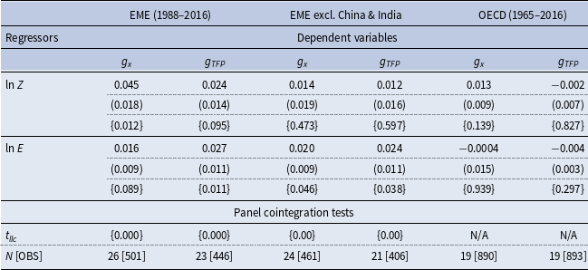
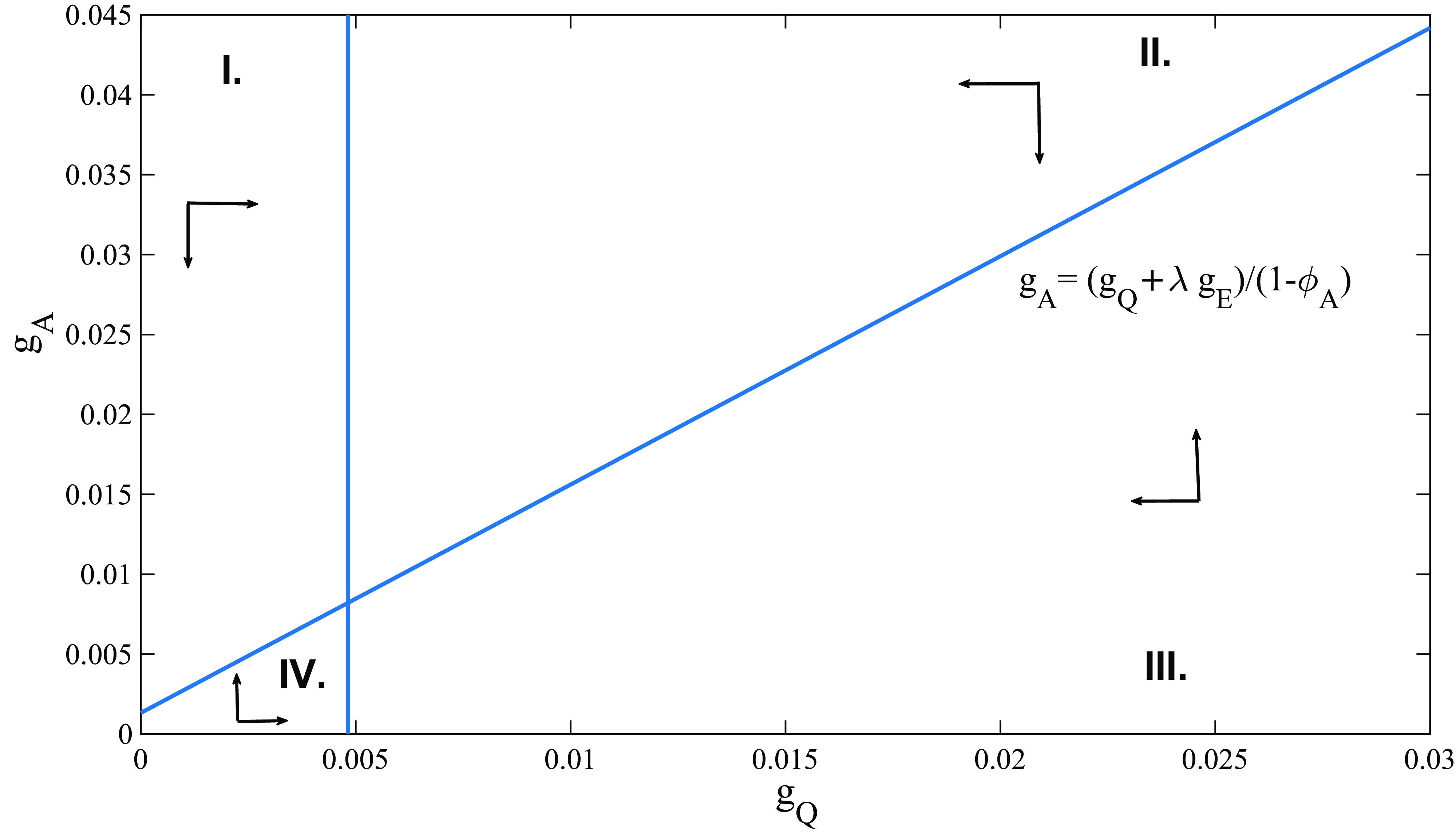
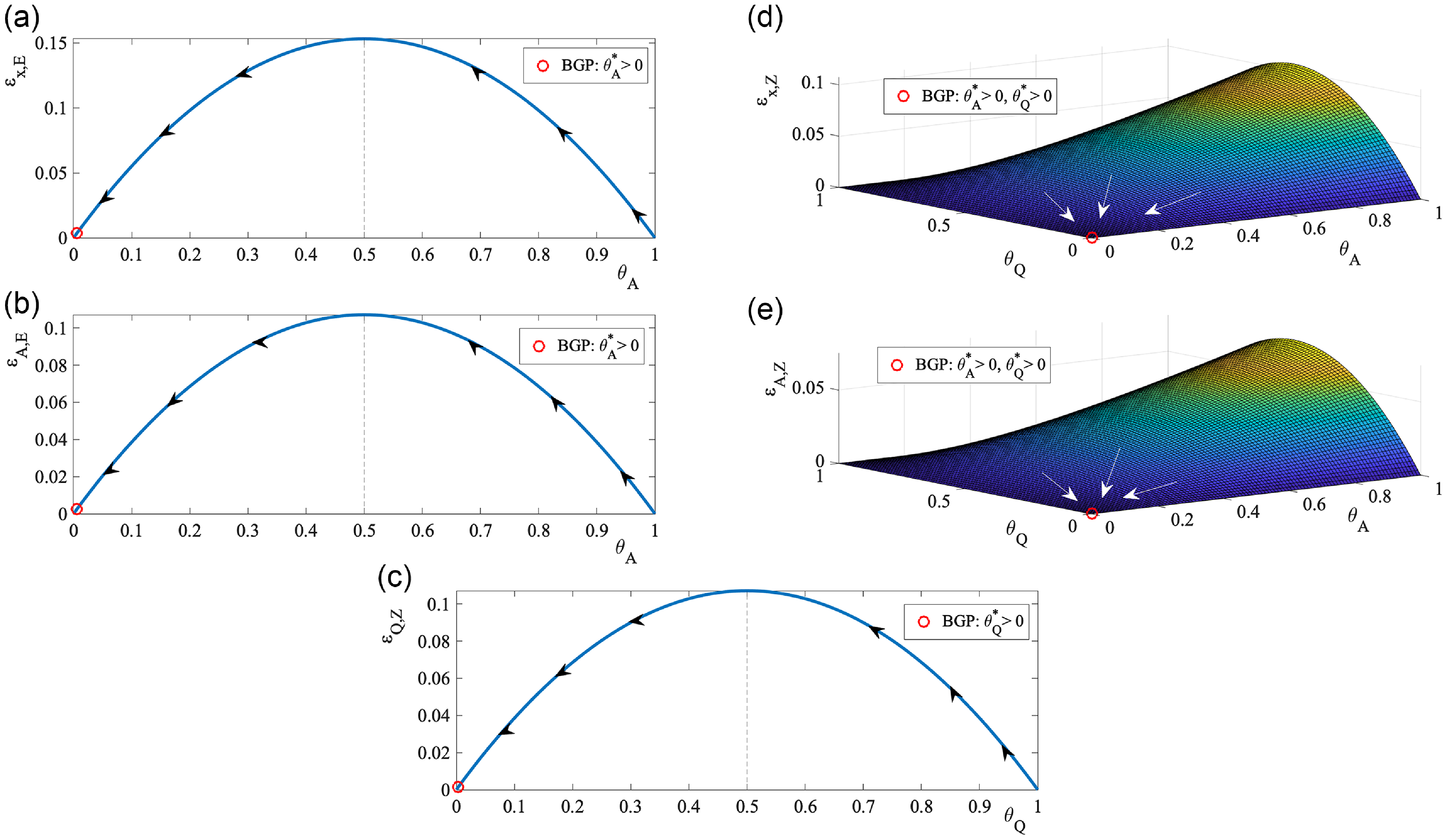
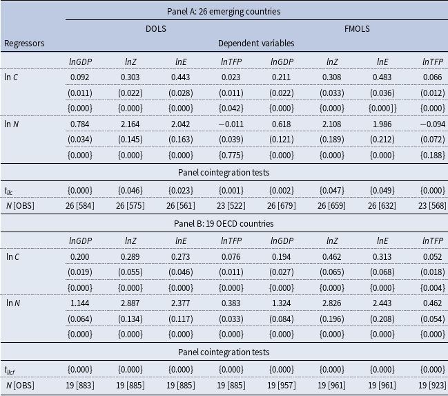
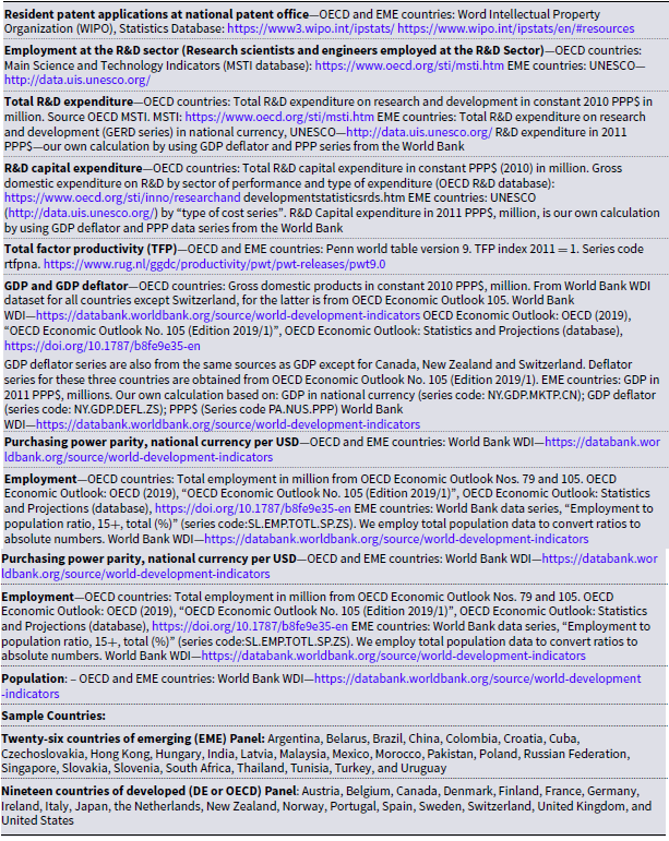
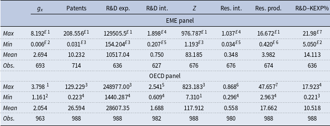


 Open access