





1. Introduction
The interface between geodesy and astrophysics is realised through the Very Long Baseline Interferometry (VLBI) radio sources that constitute the International Celestial Reference Frame (ICRF). For geodesy, the primary requirement is stationarity; however, the reference sources that make up the ICRF are mostly radio-loud Active Galactic Nuclei (AGN), which can exhibit intrinsic changes in structure and flux over time and across frequency, manifesting as apparent shifts in their astrometric positions. The vast majority of the ICRF radio-loud AGN included in this study are blazars, AGN whose relativistic jets are aligned close to the line of sight. These sources are physically dynamic, exhibiting flares, ejecting new jet components, and showing frequency-dependent structures. Because blazars dominate the extragalactic $\gamma$
-ray sky, they provide a natural class in which to investigate connections between high-energy emission and astrometric radio variability.
$\gamma$
-ray sky, they provide a natural class in which to investigate connections between high-energy emission and astrometric radio variability.
Traditionally, geodesy has treated these structural changes as noise sources to be mitigated. However, the wealth of accumulated astrometric data offers a powerful tool for astrophysics. By linking the stability of the ICRF to the physics of the sources, we can probe the mechanisms of jet production. Specifically, if astrometric ‘wobbles’ are driven by the ejection of bright, optically thick jet components, the evolution of component flux densities will shift the centroid of emission. High-energy emission may serve as an early warning system for such events. $\gamma$
-ray flares, often associated with the energisation of new components near the jet base, could effectively trace the physical events that lead to apparent position shifts of the radio sources in the reference frames.
$\gamma$
-ray flares, often associated with the energisation of new components near the jet base, could effectively trace the physical events that lead to apparent position shifts of the radio sources in the reference frames.
It is well known that the position of the brightest component in a VLBI image which is usually referred to as the ‘core’, may (or may not) shift over time with respect to the launching point of the jet (Niinuma et al. Reference Niinuma, Kino, Doi, Hada, Nagai and Koyama2015; Koyama et al. Reference Koyama2019). This position also often changes as a function of frequency: the well-known ‘core-shift’ effect. This is a consequence of the synchrotron self-absorbed (SSA) emission occurring close to a blazar jet base having its surface of last scattering ( $\tau=1$
) surface change as a function of frequency (e.g. Lobanov Reference Lobanov1998). Interpreting the ‘core-shift’ effect assumes a freely expanding conical jet that, amongst other things, depends on the magnetic field strength and the particle number density (Blandford & Königl Reference Blandford and Königl1979).
$\tau=1$
) surface change as a function of frequency (e.g. Lobanov Reference Lobanov1998). Interpreting the ‘core-shift’ effect assumes a freely expanding conical jet that, amongst other things, depends on the magnetic field strength and the particle number density (Blandford & Königl Reference Blandford and Königl1979).
Many studies have been conducted, looking for and finding the ‘core-shift’ effect but have typically been single-epoch studies (Kovalev et al. Reference Kovalev, Lobanov, Pushkarev and Zensus2008; O’Sullivan & Gabuzda Reference O’Sullivan and Gabuzda2009; Pushkarev et al. Reference Pushkarev, Hovatta, Kovalev, Lister, Lobanov, Savolainen and Zensus2012; Fromm et al. Reference Fromm, Perucho, Ros, Savolainen and Zensus2015; Mohan et al. Reference Mohan2015; Algaba et al. Reference Algaba, Nakamura, Asada and Lee2017; Pushkarev et al. Reference Pushkarev, Butuzova, Kovalev and Hovatta2019). While more recently, variability of the ‘core-shift’ effect as a function of time has been investigated and found by Lisakov et al. (Reference Lisakov, Kovalev, Savolainen, Hovatta and Kutkin2017), Plavin et al. (Reference Plavin, Kovalev, Pushkarev and Lobanov2019), Sharma et al. (Reference Sharma, Massi and Torricelli-Ciamponi2022), Chamani et al. (Reference Chamani, Savolainen, Ros, Kovalev, Wiik, Lähteenmäki, Tornikoski and Tammi2023). The favoured interpretation of this variability is either changes in the magnetic field strength or the particle number density, with perhaps changes in particle number densities preferred (Plavin et al. Reference Plavin, Kovalev, Pushkarev and Lobanov2019).
It is important to note that the SSA interpretation of the brightest component in VLBI maps is likely true only at cm wavelengths. At mm-wave, it has been suggested that the brightest component is a standing shock (e.g. Jorstad et al. Reference Jorstad2017). If this is the case, the ‘core-shift’ effect would not be expected and may not be observed (Hodgson et al. Reference Hodgson2017; Dodson et al. Reference Dodson, Rioja, Molina and Gómez2017).
While this variability is undesirable for geodesy (see: Chamani et al. Reference Chamani, Savolainen, Ros, Kovalev, Wiik, Lähteenmäki, Tornikoski and Tammi2023, for a detailed discussion), this variability also allows us to explore the emission mechanisms of higher energy light by exploring correlations with this temporal variability. In this paper, we investigate near-in-time $\gamma$
-ray fluxes with time-dependent changes of the brightest component relative to the ICRF.
$\gamma$
-ray fluxes with time-dependent changes of the brightest component relative to the ICRF.
2. Methods and observations
We began with a sample of 92 sources that were being monitored as part of the K-band Astro2Geo VLBI observing project (Hodgson et al. Reference Hodgson, L’Huillier, Liodakis, Lee and Shafieloo2020, Reference Hodgson, L’Huillier, Liodakis, Lee and Shafieloo2023; de Witt et al. Reference de Witt, Jacobs, Gordon, Bietenholz, Nickola and Bertarini2023a
). The sources were selected for being easily detectable and with large amounts of existing data. In addition, we added selected sources with large astrometric offset variability (with weighted standard deviation of position time series of several tenths of mas) as reported, for example, by Cigan et al. (Reference Cigan, Makarov, Secrest, Gordon, Johnson and Lambert2024), Krásná et al. (Reference Krásná, Jacobs, Schartner and Charlot2025) for which K-band data were available ( $0119+115$
,
$0119+115$
, $0229+131$
,
$0229+131$
, $0642+449$
). This leads to a natural bias, and thus any results should not be interpreted as typical of the general AGN population.
$0642+449$
). This leads to a natural bias, and thus any results should not be interpreted as typical of the general AGN population.
The position offsets with respect to the third realisation of the ICRF at 8.4 GHz (ICRF3-SX; Charlot et al. Reference Charlot2020) were calculated for both S/X band (2.3/8.4 GHz) and K-band (24 GHz) VLBI data in a geodetic/astrometric analysis. We analysed all 24-h VLBI S/X sessions provided through the International VLBI Service for Geodesy and Astrometry (IVS; Nothnagel et al. Reference Nothnagel, Artz, Behrend and Malkin2017) Data Centers (Noll Reference Noll2010) starting from 1980.0 until 2024.0. This is a heterogeneous dataset of global VLBI sessions consisting of several programmes with different observation goals, such as providing rapid Earth orientation parameters, maintenance of terrestrial reference frame, or maintenance and expansion of celestial reference frame. Therefore, the uncertainty of estimated parameters, such as source coordinates, varies from session to session based mainly on the terrestrial network involved. On the other hand, analysed 24-h K-band sessions were provided through the Astro2GeoFootnote
a
project, including the earlier pilot sessions (Lanyi et al. Reference Lanyi2010; Petrov et al. Reference Petrov, Kovalev, Fomalont and Gordon2011) run with Very Long Baseline Array (VLBA) between 2002 and 2008. Thirteen years later, building from this foundation, a new collaboration accomplished a renewal of regular observations at 24 GHz with VLBA comprising ten 25-m dishes on the US territory providing homogenous VLBI sessions with the primary aim of enhancing the source density and sky coverage and improving the astrometric accuracy of the K-band position catalogue. Further stations (HartRAO in South Africa, Hobart in Tasmania, Yebes in Spain, Mopra in Australia) have joined the K-band Astro2Geo VLBI Project, observing with a core network built from Korean VLBI telescopes since 2022. We processed the VLBI group delays, fundamental observables of geodetic and global astrometric VLBI, which are provided after correlation, fringe fitting, and basic pre-processing. The analysis was done with the Vienna VLBI and Satellite Software (VieVS; Böhm et al. Reference Böhm2018) following the current International Earth Rotation and Reference Systems Service (IERS) Conventions 2020 (Petit & Luzum Reference Petit and Luzum2010) with their updates. A priori models and parametrisation of the single session solution followed the setup described in Krásná et al. (Reference Krásná2023a
) for S/X sessions and in Krásná et al. (Reference Krásná, Gordon, de Witt and Jacobs2023b
) for K-band sessions. The a priori positions of the antennas were modelled in International Terrestrial Reference Frame 2020 (ITRF2020) (Altamimi et al. Reference Altamimi, Rebischung, Collilieux, Métivier and Chanard2023) with the position offset at epoch 2015.0, the linear velocity accounting for continental drift, and with post-seismic deformation model at stations subjected to major earthquakes. The a priori locations of radio sources were taken from ICRF3-SX accounting for the solar system barycentre acceleration with the recommended amplitude of 5.8 $\unicode{x03BC}$
as/y in direction to Galactic centre. In order to avoid any distortion of the source position estimates of interest, we did not follow the standard procedure for the definition of the celestial reference frame datum, which suggests applying the no-net-rotation condition (Jacobs et al. Reference Jacobs, Heflin, Lanyi, Sovers, Steppe, Behrend and Baver2010) on radio source positions with respect to the defining sources of the a priori catalogue. Instead, we estimated the session-wise corrections to source positions in right ascension and declination (
$\unicode{x03BC}$
as/y in direction to Galactic centre. In order to avoid any distortion of the source position estimates of interest, we did not follow the standard procedure for the definition of the celestial reference frame datum, which suggests applying the no-net-rotation condition (Jacobs et al. Reference Jacobs, Heflin, Lanyi, Sovers, Steppe, Behrend and Baver2010) on radio source positions with respect to the defining sources of the a priori catalogue. Instead, we estimated the session-wise corrections to source positions in right ascension and declination ( $\Delta \mathrm{RA}$
,
$\Delta \mathrm{RA}$
, $\Delta \mathrm{Dec}$
) of the selected 92 sources without any constraints. The positions of the remaining sources in the session were fixed to their a priori values. The magnitude of the position offset (i.e. the angular separation) was calculated by
$\Delta \mathrm{Dec}$
) of the selected 92 sources without any constraints. The positions of the remaining sources in the session were fixed to their a priori values. The magnitude of the position offset (i.e. the angular separation) was calculated by $((\Delta \mathrm{RA}\cdot \cos\mathrm{Dec})^{2} + \Delta \mathrm{Dec}^{2})^{1/2}$
. The formal errors of the position estimates were taken into account and propagated through the analysis.
$((\Delta \mathrm{RA}\cdot \cos\mathrm{Dec})^{2} + \Delta \mathrm{Dec}^{2})^{1/2}$
. The formal errors of the position estimates were taken into account and propagated through the analysis.
It is critical to note the systematic factors influencing these formal errors from single-session adjustment. The astrometric uncertainty is dependent mainly on: (i) Flux Density: Brighter sources yield higher signal-to-noise ratios (SNR), resulting in smaller formal position uncertainties; (ii) Declination: The distribution of VLBI stations heavily favours the Northern Hemisphere. Consequently, sources with low or negative declinations suffer from poorer UV-coverage, resulting in elongated synthesised beams and larger position uncertainties in the declination component; (iii) Number of Observations: Higher number of observations reduces statistical error, but it varies between individual sessions; and (iv) Station network geometry: Short baseline leads to a low angle of intersection, which causes a high uncertainty in the source position estimates.
Despite measuring K-band flux densities, we lack contemporaneous S/X band flux density information for all epochs. This limitation prevents a full spectral index analysis at this stage. It may be analysed in the future if full flux density data become available.
We obtained Fermi-LAT light curves from the Fermi Light-Curve Repository (Abdollahi et al. Reference Abdollahi2023). The LAT continually scans the entire sky, covering an energy range from 20 MeV to $\gt$
300 GeV, providing regular monitoring of our target sources. After performing the recommended validation work on these data (Abdollahi et al. Reference Abdollahi2023), we extracted 30-day cadence light curves to roughly align with the VLBI observation cadence, applying a 2-
$\gt$
300 GeV, providing regular monitoring of our target sources. After performing the recommended validation work on these data (Abdollahi et al. Reference Abdollahi2023), we extracted 30-day cadence light curves to roughly align with the VLBI observation cadence, applying a 2- $\sigma$
detection threshold and leaving the spectral index free in the fit. We then matched near-in-time
$\sigma$
detection threshold and leaving the spectral index free in the fit. We then matched near-in-time $\gamma$
-ray fluxes that were within
$\gamma$
-ray fluxes that were within $\pm$
30 days of the VLBI observations. If multiple
$\pm$
30 days of the VLBI observations. If multiple $\gamma$
-ray fluxes fell within this window, the nearest-in-time observation was selected. While shorter windows (e.g. 14 days) were considered for high-cadence sources, the 30-day window provided the most robust overlap for the full sample.
$\gamma$
-ray fluxes fell within this window, the nearest-in-time observation was selected. While shorter windows (e.g. 14 days) were considered for high-cadence sources, the 30-day window provided the most robust overlap for the full sample.
To account for the left-censoring of the $\gamma$
-ray data and avoid truncation bias, upper limits were retained. We implemented an Expectation-Maximisation (EM) algorithm adapted for Orthogonal Distance Regression (ODR). Instead of dropping non-detections, this approach treats them as left-censored data points, iteratively calculating the expected value of the true flux using a truncated normal distribution based on the radio offsets and the upper limits (see Isobe et al. Reference Isobe, Feigelson and Nelson1986, for a detailed explanation). Data with relative errors
$\gamma$
-ray data and avoid truncation bias, upper limits were retained. We implemented an Expectation-Maximisation (EM) algorithm adapted for Orthogonal Distance Regression (ODR). Instead of dropping non-detections, this approach treats them as left-censored data points, iteratively calculating the expected value of the true flux using a truncated normal distribution based on the radio offsets and the upper limits (see Isobe et al. Reference Isobe, Feigelson and Nelson1986, for a detailed explanation). Data with relative errors $\gt100\%$
were excluded unless they were designated as upper limits. Sources with at least one bin detected within the window (with the nearest-in-time used for the analysis) are given in Table 1 along with their redshift and correlation slopes and p-values. The fit was performed taking into account errors in both variables. Significant (
$\gt100\%$
were excluded unless they were designated as upper limits. Sources with at least one bin detected within the window (with the nearest-in-time used for the analysis) are given in Table 1 along with their redshift and correlation slopes and p-values. The fit was performed taking into account errors in both variables. Significant ( $p\lt0.05$
) correlations are bolded. In total, 57 sources were found.
$p\lt0.05$
) correlations are bolded. In total, 57 sources were found.
Results of the correlation analysis for the cross-matched IVS and Fermi-LAT (4FGL) source sample. Superscript numbers in the redshift column correspond to the literature references. Redshift references: [1] Pursimo et al. (Reference Pursimo2013); [2]; Jones et al. (Reference Jones2009); [3] Drinkwater et al. (Reference Drinkwater1997); [4] MAGIC Collaboration et al. (2018); [5] Burbidge (Reference Burbidge1970); [6] de Veny et al. (Reference de Veny, Osborn and Janes1971); [7] Furniss et al. (Reference Furniss, Worseck, Fumagalli, Johnson, Williams, Pontrelli and Prochaska2019); [8] Junkkarinen (Reference Junkkarinen1984); [9] Healey et al. (Reference Healey2008); [10] McIntosh et al. (Reference McIntosh, Rix, Rieke and Foltz1999); [11] photometric estimate from OCARS: Flesch (Reference Flesch2023); [12] Smith & Spinrad (Reference Smith and Spinrad1980); [13] Falomo et al. (Reference Falomo, Pesce and Treves1993); [14] Vermeulen et al. (Reference Vermeulen, Ogle, Tran, Browne, Cohen, Readhead, Taylor and Goodrich1995); [15] Schmidt (Reference Schmidt1965).

Table 1. Long description
The image contains six graphs. The top left graph is a scatter plot showing the correlation between gamma-ray flux and S/X band offsets with respect to ICRF. The red line represents the survivor-bias corrected best fit, while the grey dashed line shows the non-corrected fit. Blue marks indicate detections, and grey marks indicate upper limits. The top right graph is a zDCF plot for S/X band with significance levels indicated by yellow, green, and red lines. The middle row contains similar graphs for the K-band. The bottom row shows two line graphs: the left graph overlays monthly-binned gamma-ray flux in blue with S/X band offsets in grey, and the right graph overlays monthly-binned gamma-ray flux with K-band offsets. The graphs illustrate the variability of the core-shift effect over time and its correlation with gamma-ray flux.
In Figure 1 we show an example plot of the analysis. Further plots are given in Appendix A. In the top left is the S/X band correlation plot in log scale, now displaying both detections and upper limits. The original linear fit is shown alongside the new EM-corrected fit. Below is the same for K-band.
Example plot for 0016+731. Top left: S/X band correlation plot. The Survivor-bias (SC) corrected best fit is in red with 1, 2 and 3 $\sigma$
errors in grey. The grey dashed line is the non corrected fit. Blue marks are detection and grey marks are upper limits. Top right: zDCF at S/X band with 1 (yellow), 2 (green) and 3 (red)
$\sigma$
errors in grey. The grey dashed line is the non corrected fit. Blue marks are detection and grey marks are upper limits. Top right: zDCF at S/X band with 1 (yellow), 2 (green) and 3 (red) $\sigma$
significance levels indicated. Note that zDCF panels may be empty (particularly at K-band) for sources with little data. Additionally, the 1, 2, and 3
$\sigma$
significance levels indicated. Note that zDCF panels may be empty (particularly at K-band) for sources with little data. Additionally, the 1, 2, and 3 $\sigma$
significance contours (derived simulated light curves) may span a wider range of lag times than the real data; hence, these bounds can extend across the plot even in cases where the real data only yields one or two valid zDCF points. Middle row: Same as top row but for K-band. Bottom: monthly-binned
$\sigma$
significance contours (derived simulated light curves) may span a wider range of lag times than the real data; hence, these bounds can extend across the plot even in cases where the real data only yields one or two valid zDCF points. Middle row: Same as top row but for K-band. Bottom: monthly-binned $\gamma$
-ray flux (blue) overplotted with the S/X band offsets (left) and with the K-band offsets (right) with respect to the ICRF3-SX.
$\gamma$
-ray flux (blue) overplotted with the S/X band offsets (left) and with the K-band offsets (right) with respect to the ICRF3-SX.

Figure 1. Long description
The image contains six graphs. The top left graph is a scatter plot showing the correlation between gamma-ray flux and S/X band offsets with respect to ICRF. The red line represents the survivor-bias corrected best fit, while the grey dashed line shows the non-corrected fit. Blue marks indicate detections, and grey marks indicate upper limits. The top right graph is a zDCF plot for S/X band with significance levels indicated by yellow, green, and red lines. The middle row contains similar graphs for the K-band. The bottom row shows two line graphs: the left graph overlays monthly-binned gamma-ray flux in blue with S/X band offsets in grey, and the right graph overlays monthly-binned gamma-ray flux with K-band offsets. The graphs illustrate the variability of the core-shift effect over time and its correlation with gamma-ray flux.
We then investigated any possible time-delay between variations in the positional offsets with respect to the ICRF3-SX and $\gamma$
-ray fluxes by computing the Discrete Correlation Function (DCF) using the open zDCF package (Alexander Reference Alexander2014). Because the DCF relies mathematically on known variances and discrete pairings, this temporal analysis was restricted strictly to
$\gamma$
-ray fluxes by computing the Discrete Correlation Function (DCF) using the open zDCF package (Alexander Reference Alexander2014). Because the DCF relies mathematically on known variances and discrete pairings, this temporal analysis was restricted strictly to $\gamma$
-ray detections to avoid introducing model-dependent variance from imputed limits. Significances were calculated by simulating the
$\gamma$
-ray detections to avoid introducing model-dependent variance from imputed limits. Significances were calculated by simulating the $\gamma$
-ray light curves 10 000 times using the DELCgen code, recomputing the zDCF for each simulated light curve, and taking the 68, 95, and 99.7% percentiles for each lag bin. Example results of this analysis are shown in Figure 1(b) and (c) with 1, 2, and 3
$\gamma$
-ray light curves 10 000 times using the DELCgen code, recomputing the zDCF for each simulated light curve, and taking the 68, 95, and 99.7% percentiles for each lag bin. Example results of this analysis are shown in Figure 1(b) and (c) with 1, 2, and 3 $\sigma$
significance levels indicated. In the bottom row, we present the time series data using twin axes: the monthly-binned
$\sigma$
significance levels indicated. In the bottom row, we present the time series data using twin axes: the monthly-binned $\gamma$
-ray fluxes (including upper limits) are plotted alongside the S/X band (left) and K-band (right) positional offsets.
$\gamma$
-ray fluxes (including upper limits) are plotted alongside the S/X band (left) and K-band (right) positional offsets.
3. Results and discussion
We find a high proportion of statistically significant correlation between radio core astrometric offsets and $\gamma$
-ray fluxes within
$\gamma$
-ray fluxes within $\sim$
30 days of VLBI observations. Approximately 90% of sources show a significant power-law relationship (
$\sim$
30 days of VLBI observations. Approximately 90% of sources show a significant power-law relationship ( $p\lt0.05$
) in at least one of S/X or K-bands. We emphasise that the sample is biased towards sources with extensive K-band astrometric observations, with a few additional sources included because they exhibit large position offsets, and therefore the results should not be interpreted as representative of the entire blazar or broader AGN population.
$p\lt0.05$
) in at least one of S/X or K-bands. We emphasise that the sample is biased towards sources with extensive K-band astrometric observations, with a few additional sources included because they exhibit large position offsets, and therefore the results should not be interpreted as representative of the entire blazar or broader AGN population.
3.1. Comparison with the OCARS catalogue
To investigate this bias, we compared our 92 selected sources against the full Optical Characteristics of Astrometric Radio Sources (OCARS) catalogue (Malkin Reference Malkin2018). We performed two-sample Kolmogorov–Smirnov (K–S) tests on the observational parameters supplied in the OCARS catalogue in order to determine if the subset distributions differ significantly from the parent population. The results are summarised in Table 2.
The most significant deviations are found in astrometric precision and optical brightness. The subset exhibits a median semi-major axis error of 0.032 mas compared to the parent median of 1.377 mas ( $p \lt 10^{-78}$
), this tells us that our sample represents the astrometrically cleaner sample. Similarly, the subset is significantly brighter in the optical regime, with a median magnitude of 17.1 compared to the parent median of 19.4 (
$p \lt 10^{-78}$
), this tells us that our sample represents the astrometrically cleaner sample. Similarly, the subset is significantly brighter in the optical regime, with a median magnitude of 17.1 compared to the parent median of 19.4 ( $p \lt 10^{-14}$
). Spatially, we find a statistically significant difference in the distribution of Galactic Latitudes (
$p \lt 10^{-14}$
). Spatially, we find a statistically significant difference in the distribution of Galactic Latitudes ( $p \approx 0.001$
).
$p \approx 0.001$
).
However, we note that the redshift distributions show no statistically significant difference between our subset and the parent catalogue. This implies that while our sample is biased towards brighter and more compact radio sources, it remains representative of the general AGN population in terms of cosmological distance and epoch.
3.2. Physical interpretation
The physical nature of this correlation is complex. Out of the 57 analysed sources, 43 exhibit a statistically significant correlation ( $p \lt 0.05$
) in the S/X-band (13 positive, 30 negative), while 38 are significant in the K-band (16 positive, 22 negative). The slightly lower incidence of significant correlations at K-band is observationally expected; the S/X-band data goes back to 1980, whereas regular K-band observations only began in 2016. The resulting lower number of epochs in K-band reduces statistical power, making it harder to cross the
$p \lt 0.05$
) in the S/X-band (13 positive, 30 negative), while 38 are significant in the K-band (16 positive, 22 negative). The slightly lower incidence of significant correlations at K-band is observationally expected; the S/X-band data goes back to 1980, whereas regular K-band observations only began in 2016. The resulting lower number of epochs in K-band reduces statistical power, making it harder to cross the $p \lt 0.05$
threshold.
$p \lt 0.05$
threshold.
Assuming independence, selecting 43 and 38 sources from a population of 57 yields an expected overlap of roughly 29 sources. We observe 32 sources that are statistically significant in both bands. Because this excess is marginal ( $\sim$ $2 \sigma$
) and while this might be partially driven by the limited K-band time baseline, the current data does not support a strongly predictive, universal link between the two bands. Furthermore, among the 32 overlapping sources, we observe opposite correlation signs in approximately 40% (13/32) of the cases.
$2 \sigma$
) and while this might be partially driven by the limited K-band time baseline, the current data does not support a strongly predictive, universal link between the two bands. Furthermore, among the 32 overlapping sources, we observe opposite correlation signs in approximately 40% (13/32) of the cases.
That we see opposite correlations within the same source could be due to the SSA turnover frequency being sometimes above 8 GHz and below 22 GHz, therefore leading to the brightest position in the source being different at different frequencies, but the $\gamma$
-ray emission site is the same. When the
$\gamma$
-ray emission site is the same. When the $\gamma$
-ray emission site is located further downstream from the ‘normal’ ICRF position, this will be reflected as a positive correlation. If the ‘normal’ location is already downstream and then the
$\gamma$
-ray emission site is located further downstream from the ‘normal’ ICRF position, this will be reflected as a positive correlation. If the ‘normal’ location is already downstream and then the $\gamma$
-rays are then coming ‘upstream’ of this position, we would observe a negative correlation. When the SSA turnover frequency is above 8 GHz and below 22 GHz, the correlation will go in opposite directions. Indeed, such a situation was recently reported by de Witt et al. (Reference de Witt, Jacobs, Gordon, Hunt, Johnson, Armstrong, Behrend and Baver2023b
).
$\gamma$
-rays are then coming ‘upstream’ of this position, we would observe a negative correlation. When the SSA turnover frequency is above 8 GHz and below 22 GHz, the correlation will go in opposite directions. Indeed, such a situation was recently reported by de Witt et al. (Reference de Witt, Jacobs, Gordon, Hunt, Johnson, Armstrong, Behrend and Baver2023b
).
3.2.1 Multiple $\gamma$
-ray emission sites
$\gamma$
-ray emission sites

Blazar jets having $\gamma$
-rays occurring in multiple locations (e.g. in the ‘core’ and downstream quasi-stationary features) is well documented in sources such as CTA 102, OJ 287, 3C 84, and PKS 1510-089 (Schinzel et al. Reference Schinzel, Lobanov, Taylor, Jorstad, Marscher and Zensus2012; Hodgson et al. Reference Hodgson2017, Reference Hodgson2018; Orienti et al. Reference Orienti, Venturi, Dallacasa, D’Ammando, Giroletti, Giovannini, Vercellone and Tavani2011; Marscher et al. Reference Marscher2010). Such shifts in
$\gamma$
-rays occurring in multiple locations (e.g. in the ‘core’ and downstream quasi-stationary features) is well documented in sources such as CTA 102, OJ 287, 3C 84, and PKS 1510-089 (Schinzel et al. Reference Schinzel, Lobanov, Taylor, Jorstad, Marscher and Zensus2012; Hodgson et al. Reference Hodgson2017, Reference Hodgson2018; Orienti et al. Reference Orienti, Venturi, Dallacasa, D’Ammando, Giroletti, Giovannini, Vercellone and Tavani2011; Marscher et al. Reference Marscher2010). Such shifts in $\gamma$
-ray production sites would naturally explain a correlation between
$\gamma$
-ray production sites would naturally explain a correlation between $\gamma$
-ray flux and the position of the radio core.
$\gamma$
-ray flux and the position of the radio core.
The four sources above are included in our analysis. In OJ 287, we find a significant correlation, but with no time-delay. In contrast, 3C 84 shows no significant near-in-time correlation, but hints of a time-delayed correlation. CTA 102 shows a strong correlation at K-band, but inconclusive evidence of a time-delayed correlation.
From this analysis alone, we cannot provide unambiguous evidence of this mechanism and detailed source-by-source analysis of VLBI maps would be required, which is beyond the scope of this work.
3.2.2. Changes in radio core opacity
Changes in the physical conditions at the base of the jet, such as the particle density or magnetic field can alter the opacity of the radio core. This would manifest itself as a changing position of the $\tau=1$
surface – commonly observed as core-shift (Plavin et al. Reference Plavin, Kovalev, Pushkarev and Lobanov2019). If these changes are linked to
$\tau=1$
surface – commonly observed as core-shift (Plavin et al. Reference Plavin, Kovalev, Pushkarev and Lobanov2019). If these changes are linked to $\gamma$
-ray flaring, a correlation would be expected. Chamani et al. (Reference Chamani, Savolainen, Ros, Kovalev, Wiik, Lähteenmäki, Tornikoski and Tammi2023) found evidence that core-shift variability is connected to core-flux variability consistent with the predictions of Blandford & Königl (Reference Blandford and Königl1979) and similarly would naturally explain the correlations.
$\gamma$
-ray flaring, a correlation would be expected. Chamani et al. (Reference Chamani, Savolainen, Ros, Kovalev, Wiik, Lähteenmäki, Tornikoski and Tammi2023) found evidence that core-shift variability is connected to core-flux variability consistent with the predictions of Blandford & Königl (Reference Blandford and Königl1979) and similarly would naturally explain the correlations.
To test this, we compared our correlation strengths with the core-shift measurements from Plavin et al. (Reference Plavin, Kovalev, Pushkarev and Lobanov2019) for the 11 sources common to both samples, with the results shown in Figure 2 (left). We find no statistically significant correlation ( $p\approx 0.11$
) between the median core-shift magnitude and the strength of the
$p\approx 0.11$
) between the median core-shift magnitude and the strength of the $\gamma$
-ray-offset correlation. There is similarly no evidence for a link between the
$\gamma$
-ray-offset correlation. There is similarly no evidence for a link between the $\gamma$
-ray-offset and the peak-to-peak variability of the core-shift. This suggests that simple changes in average core-shift properties, at least for the 11 sources in common with Plavin et al. (Reference Plavin, Kovalev, Pushkarev and Lobanov2019), are not the likely to be the primary mechanism for the correlation.
$\gamma$
-ray-offset and the peak-to-peak variability of the core-shift. This suggests that simple changes in average core-shift properties, at least for the 11 sources in common with Plavin et al. (Reference Plavin, Kovalev, Pushkarev and Lobanov2019), are not the likely to be the primary mechanism for the correlation.
Left: Correlation plots between the median core-shift (as reported by Plavin et al. Reference Plavin, Kovalev, Pushkarev and Lobanov2019) with the strength of the ICRF3-SX offset correlation at S/X-band (top-left) and K-band (top right). The same but with the peak-to-peak core-shift variability for S/X band (bottom-left) and K-band (bottom right). Right, upper: ICRF3-SX offset vs the standard deviation of the PA from de Witt et al. (Reference de Witt, Jacobs, Gordon, Bietenholz, Nickola and Bertarini2023a
) at S/X band. Right, lower: same as top but for K band. In all panels, the red solid line represents the line of best fit, while the three progressively lighter shades of grey indicate the 1 $\sigma$
, 2
$\sigma$
, 2 $\sigma$
, and 3
$\sigma$
, and 3 $\sigma$
uncertainty ranges (confidence intervals) of the fit, respectively.
$\sigma$
uncertainty ranges (confidence intervals) of the fit, respectively.

Figure 2. Long description
The image contains six graphs. The left side features four scatter plots with error bars and a red line of best fit. The top-left plot shows the correlation between median core-shift and the strength of the ICRF3-SX offset correlation at S/X-band, while the top-right plot shows the same correlation at K-band. The bottom-left plot illustrates the correlation between peak-to-peak core-shift variability and the strength of the ICRF3-SX offset correlation at S/X-band, and the bottom-right plot shows this correlation at K-band. The right side features two scatter plots with a red line of best fit and shaded uncertainty ranges. The top-right plot shows the ICRF3-SX offset versus the standard deviation of the position angle at S/X-band, and the bottom-right plot shows the same relationship at K-band. The red line represents the line of best fit, and the grey shades indicate the 1, 2, and 3 uncertainty ranges of the fit.
3.2.3. Changes in jet Position Angle
If the jet physically changes its orientation on the sky (i.e. its Position Angle, PA), the measured position of the core could change relative to its average ICRF position. If this jet wobbling is connected to the events causing the $\gamma$
-ray flaring, a correlation could arise as has been suggested by Rani et al. (Reference Rani, Krichbaum, Marscher, Jorstad, Hodgson, Fuhrmann and Zensus2014) and Raiteri et al. (Reference Raiteri2017).
$\gamma$
-ray flaring, a correlation could arise as has been suggested by Rani et al. (Reference Rani, Krichbaum, Marscher, Jorstad, Hodgson, Fuhrmann and Zensus2014) and Raiteri et al. (Reference Raiteri2017).
To test this, we used the jet PA measurements from de Witt et al. (Reference de Witt, Jacobs, Gordon, Bietenholz, Nickola and Bertarini2023a ) and compared the standard deviation of the PA (as a proxy for variability) against our measured correlation slopes (see Figure 2, right). We find no significant correlations at S/X band or K-band. Therefore, we conclude that PA changes are likely not driving the correlations.
3.2.4. Time-delayed correlations
A time-lag between astrometric shifts and $\gamma$
-ray flux variability could constrain the relative locations of their emission regions. For example,
$\gamma$
-ray flux variability could constrain the relative locations of their emission regions. For example, $\gamma$
-ray flares are often observed to lead radio flares by several months, suggesting that they occur closer to the jet base than the radio core (e.g. Max-Moerbeck et al. Reference Max-Moerbeck, Richards, Hovatta, Pavlidou, Pearson and Readhead2014; Fuhrmann et al. Reference Fuhrmann2014; Ramakrishnan et al. Reference Ramakrishnan, Hovatta, Nieppola, Tornikoski, Lähteenmäki and Valtaoja2015). The simplistic view suggests that an event causes a
$\gamma$
-ray flares are often observed to lead radio flares by several months, suggesting that they occur closer to the jet base than the radio core (e.g. Max-Moerbeck et al. Reference Max-Moerbeck, Richards, Hovatta, Pavlidou, Pearson and Readhead2014; Fuhrmann et al. Reference Fuhrmann2014; Ramakrishnan et al. Reference Ramakrishnan, Hovatta, Nieppola, Tornikoski, Lähteenmäki and Valtaoja2015). The simplistic view suggests that an event causes a $\gamma$
-ray flare close to the core, followed by a rising radio flux as a new jet component emerges and moves downstream. To search for a similar relationship with astrometric positions, we performed a cross-correlation analysis using zDCF. We find tentative evidence (
$\gamma$
-ray flare close to the core, followed by a rising radio flux as a new jet component emerges and moves downstream. To search for a similar relationship with astrometric positions, we performed a cross-correlation analysis using zDCF. We find tentative evidence ( $\gt$
$\gt$ $2 \sigma$
) for time offsets in only 5 sources (
$2 \sigma$
) for time offsets in only 5 sources ( $0133+476, 0235+164, 1424-418$
, 3C 120, and 3C 84). However, these detections are not robust and in some cases imply an astrophysically challenging delay on the order of years. The fact that we only see this in five sources suggests that the simplistic view of delayed structural evolution is likely incomplete or easily masked by multiple flaring locations. The dominant signal across the population (consistent across both S/X and K-bands) appears to be from correlations within our 60-day window. However, an analysis in this way is obviously limited, and future analysis with radio flux density information would be valuable.
$0133+476, 0235+164, 1424-418$
, 3C 120, and 3C 84). However, these detections are not robust and in some cases imply an astrophysically challenging delay on the order of years. The fact that we only see this in five sources suggests that the simplistic view of delayed structural evolution is likely incomplete or easily masked by multiple flaring locations. The dominant signal across the population (consistent across both S/X and K-bands) appears to be from correlations within our 60-day window. However, an analysis in this way is obviously limited, and future analysis with radio flux density information would be valuable.
4. Conclusions
We have found a high incidence ( $\sim$
90%) of correlation between the changes in time series of radio core astrometric positions and
$\sim$
90%) of correlation between the changes in time series of radio core astrometric positions and $\gamma$
-ray fluxes in our biased sample. We have explored four potential interpretations, including multiple/changing
$\gamma$
-ray fluxes in our biased sample. We have explored four potential interpretations, including multiple/changing $\gamma$
-ray emission sites, changes in nuclear opacity, changes in radio core flux densities, and changes in PA. We find no evidence or inconclusive results for a single mechanism driving the correlations. We therefore interpret the correlations as not arising from any single universal mechanism and point towards a complex interplay of many physical factors that likely change from source to source. For some objects, shifts in the
$\gamma$
-ray emission sites, changes in nuclear opacity, changes in radio core flux densities, and changes in PA. We find no evidence or inconclusive results for a single mechanism driving the correlations. We therefore interpret the correlations as not arising from any single universal mechanism and point towards a complex interplay of many physical factors that likely change from source to source. For some objects, shifts in the $\gamma$
-ray emission sites may dominate while in others subtle opacity or structural changes in the radio core may cause the correlations. Detailed source-by-source analysis of VLBI images may be required to disentangle the mechanisms.
$\gamma$
-ray emission sites may dominate while in others subtle opacity or structural changes in the radio core may cause the correlations. Detailed source-by-source analysis of VLBI images may be required to disentangle the mechanisms.
It is important to note the limitations of this study - especially that it is a biased sample and should not be considered a representative result for the entire blazar (or AGN) population.
In future work we will more directly investigate the effects of radio emission on the correlations and furthermore will strive to do it with a more complete and unbiased sample in order to find how universal such an effect may be. Further, we will investigate effects such as source type (e.g. BL Lac vs FSRQ) and/or other properties such as jet apparent speeds.
K-S test results comparing the study subset ( $N=92$
) with the parent OCARS catalogue.
$N=92$
) with the parent OCARS catalogue.
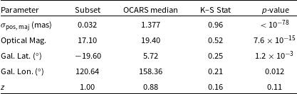
Table 2. Long description
The image contains six graphs. The left side features four scatter plots with error bars and a red line of best fit. The top-left plot shows the correlation between median core-shift and the strength of the ICRF3-SX offset correlation at S/X-band, while the top-right plot shows the same correlation at K-band. The bottom-left plot illustrates the correlation between peak-to-peak core-shift variability and the strength of the ICRF3-SX offset correlation at S/X-band, and the bottom-right plot shows this correlation at K-band. The right side features two scatter plots with a red line of best fit and shaded uncertainty ranges. The top-right plot shows the ICRF3-SX offset versus the standard deviation of the position angle at S/X-band, and the bottom-right plot shows the same relationship at K-band. The red line represents the line of best fit, and the grey shades indicate the 1, 2, and 3 uncertainty ranges of the fit.
Acknowledgements
J.A.H. acknowledges the support of the National Research Foundation of Korea (NRF) (NRF-2021R1C1C1009973). This work was supported by the National Research Foundation of Korea (NRF) grant funded by the Korea government (MSIT) RS-2025-16302968. We acknowledge use of the VLBA under the USNO’s time allocation programme since 2017. This work supports USNO’s ongoing research into the celestial reference frame and geodesy. The VLBA is operated by the National Radio Astronomy Observatory, which is a facility of the National Science Foundation operated under cooperative agreement by Associated Universities, Inc. We acknowledge use of the Hobart, HartRAO, Mopra, Yebes and Korean VLBI Network (KVN) K-band observations. We acknowledge the IVS for providing the S/X data and the Astro2Geo VLBI Project for the K-band data. We thank David Gordon (USNO) for the fringe-fitting of the VLBI K-band observations and creation of the databases.
Data availability statement
The VLBI S/X data used in this work are available from the IVS Data Centers. The K-band data are available upon request from the Astro2Geo VLBI Project. Fermi-LAT data are publicly available from the Fermi Light-Curve Repository.
Appendix A. Extended plots
Same as Figure 1, but for the source 0035 $-$
252.
$-$
252.

Figure A1. Long description
The image contains six graphs related to the source 0035252. The top left graph shows the S/X offset with respect to ICRF in milliarcseconds (mas) against gamma-ray flux in photons per square centimeter per second. The top right graph displays the Z-transformed discrete correlation function (ZDCF) for S/X against lag in days. The middle left graph presents the K offset with respect to ICRF in mas against gamma-ray flux. The middle right graph shows the ZDCF for K against lag in days. The bottom left graph illustrates the S/X offset in mas and gamma-ray flux in photons per square centimeter per second over decimal years. The bottom right graph depicts the K offset in mas and gamma-ray flux over decimal years. Each graph includes data points with error bars and trend lines.
Same as Figure 1, but for the source 0109 $+$
224.
$+$
224.

Figure A2. Long description
The image contains four graphs analyzing the positional offsets and gamma-ray flux of a blazar jet. The top left graph shows the S/X band offset with respect to the ICRF as a function of gamma-ray flux, with data points and a trend line. The top right graph displays the ZDCF (Z-transformed Discrete Correlation Function) between the S/X band offset and gamma-ray flux over a range of lags in days, with data points and confidence intervals. The bottom left graph presents the K band offset with respect to the ICRF as a function of gamma-ray flux, similar to the top left graph. The bottom right graph shows the ZDCF between the K band offset and gamma-ray flux over a range of lags in days, with data points and confidence intervals. The bottom two graphs on the left and right depict time series data of the S/X and K band offsets, respectively, along with gamma-ray flux over decimal years. The graphs illustrate the core-shift effect and the positional variability of the blazar jet components over time and frequency.
Same as Figure 1, but for the source 0133 $+$
476.
$+$
476.

Figure A3. Long description
The image contains six graphs arranged in a 2x3 grid. The top row features two line graphs showing the Z-transformed discrete correlation function (ZDCF) for S/X and K bands against lag in days. The middle row displays two scatter plots of gamma-ray flux versus positional offsets for S/X and K bands, with data points in blue and gray, and trend lines in red. The bottom row presents two time series plots of positional offsets for S/X and K bands against decimal year, with gamma-ray flux overlaid in orange. The graphs illustrate the relationship between gamma-ray flux and positional offsets over time, highlighting variations and trends in the data.
Same as Figure 1, but for the source 0138 $-$
097.
$-$
097.

Figure A4. Long description
The image contains six graphs arranged in a 2x3 grid. The top-left graph shows the positional offset in milliarcseconds (mas) of the S/X band relative to the International Celestial Reference Frame (ICRF) as a function of gamma-ray flux in photons per square centimeter per second. The data points are scattered with error bars, and a red line indicates a trend. The top-right graph displays the Z-transformed discrete correlation function (ZDCF) between the S/X band offset and gamma-ray flux over a lag period of days, with data points and confidence intervals. The middle-left graph shows the positional offset in the K band relative to the ICRF as a function of gamma-ray flux, with a similar scatter plot and trend line. The middle-right graph shows the ZDCF for the K band offset and gamma-ray flux, which appears to be flat, indicating no significant correlation. The bottom-left graph plots the S/X band offset and gamma-ray flux over time, with both datasets showing variability. The bottom-right graph plots the K band offset and gamma-ray flux over time, also showing variability. The graphs collectively illustrate the relationship and time variability of positional offsets in different bands with respect to gamma-ray flux, highlighting the core-shift effect and its potential variability over time.
Same as Figure 1, but for the source 0202 $+$
319.
$+$
319.

Figure A5. Long description
The image contains six graphs related to the source 0202319. The top left graph shows the S/X offset with respect to ICRF in milliarcseconds (mas) against gamma-ray flux in photons per square centimeter per second. The top right graph displays the ZDCF (S/X) against lag in days. The middle left graph presents the K offset with respect to ICRF in mas against gamma-ray flux. The middle right graph shows the ZDCF (K) against lag in days. The bottom left graph illustrates the S/X offset in mas over decimal years, with gamma-ray flux in photons per square centimeter per second on a secondary axis. The bottom right graph depicts the K offset in mas over decimal years, with gamma-ray flux on a secondary axis. Each graph includes data points with error bars and trend lines.
Same as Figure 1, but for the source 0234 $+$
285.
$+$
285.

Figure A6. Long description
The image contains six graphs arranged in a 2x3 grid. The top row features two scatter plots with a fitted line, showing the relationship between gamma-ray flux and positional offsets in S/X and K bands. The x-axis represents gamma-ray flux in photons per square centimeter per second, while the y-axis shows the positional offset in milliarcseconds. The middle row contains two Z-transformed discrete correlation function (ZDCF) plots, illustrating the correlation between gamma-ray flux and positional offsets over time lags in days. The bottom row presents two time series plots, displaying the positional offsets in S/X and K bands over decimal years, with gamma-ray flux overlaid in orange. The graphs collectively analyze the variability of the core-shift effect in the source 0234285, indicating potential changes in magnetic field strength or particle number density.
Same as Figure 1, but for the source 0235 $+$
164.
$+$
164.

Figure A7. Long description
The image contains four graphs related to the source 0235164. The top left graph shows the S/X offset with respect to the ICRF against gamma-ray flux, with data points and a trend line. The top right graph displays the ZDCF (S/X) against lag in days, with data points and confidence intervals. The bottom left graph presents the K offset with respect to the ICRF against gamma-ray flux, with data points and a trend line. The bottom right graph shows the ZDCF (K) against lag in days, with data points and confidence intervals. The bottom two graphs on the left and right depict the S/X and K offsets, respectively, against decimal year, with data points and gamma-ray flux overlaid. All values are approximated.
Same as Figure 1, but for the source 3C84.

Figure A8. Long description
The image contains multiple graphs analyzing the relationship between gamma-ray flux and positional offsets for the source 3C84. The top left graph is a scatter plot showing the S/X offset with respect to ICRF in milliarcseconds (mas) against gamma-ray flux in photons per square centimeter per second. The data points are accompanied by a red trend line with a shaded confidence interval. The top right graph is a ZDCF (Z-transformed Discrete Correlation Function) plot, showing the correlation between S/X offsets and gamma-ray flux over a lag period in days. The bottom left graph is another scatter plot, this time showing the K offset with respect to ICRF in mas against gamma-ray flux, with a similar red trend line and confidence interval. The bottom right graph is another ZDCF plot, showing the correlation between K offsets and gamma-ray flux over a lag period in days. The bottom two graphs on the left and right show the time series of S/X and K offsets, respectively, plotted against decimal year, with gamma-ray flux overlaid in orange. The S/X and K offsets are measured in mas, and the gamma-ray flux is measured in photons per square centimeter per second. The graphs collectively illustrate the variability and correlation between gamma-ray flux and positional offsets for the source 3C84.
Same as Figure 1, but for the source NRAO140.

Figure A9. Long description
The image contains six graphs analyzing the correlation between gamma-ray flux and radio offsets for the source NRAO140. The top left graph shows the S/X offset versus gamma-ray flux, with data points and a trend line. The top right graph displays the ZDCF (S/X) values over a range of lags in days. The middle left graph presents the K offset versus gamma-ray flux, with data points and a trend line. The middle right graph shows the ZDCF (K) values over a range of lags in days. The bottom left graph plots the S/X offset over time, with gamma-ray flux overlaid. The bottom right graph plots the K offset over time, with gamma-ray flux overlaid. The graphs illustrate the relationship between gamma-ray flux and radio offsets, highlighting trends and correlations.
Same as Figure 1, but for the source 0402 $-$
362.
$-$
362.

Figure A10. Long description
The image contains six graphs related to the analysis of gamma-ray flux and astrometric offsets for the source 0402362. The top left graph is a scatter plot showing the S/X band offset with respect to ICRF against gamma-ray flux, with data points and error bars. The top right graph is a ZDCF plot for the S/X band, displaying the correlation as a function of lag in days. The middle left graph is another scatter plot, this time showing the K band offset with respect to ICRF against gamma-ray flux. The middle right graph is a ZDCF plot for the K band, similar to the top right graph. The bottom left graph is a time series plot showing the S/X band offset over decimal years, with gamma-ray flux overlaid. The bottom right graph is a time series plot showing the K band offset over decimal years, with gamma-ray flux overlaid. Each graph includes data points, error bars, and trend lines where applicable. The graphs collectively illustrate the relationship between gamma-ray flux and astrometric offsets over time for the source 0402362.
Same as Figure 1, but for the source 0405 $-$
385.
$-$
385.

Figure A11. Long description
The image contains four graphs related to the source 0405-385. The top left graph shows the S/X offset with respect to ICRF in milliarcseconds (mas) against gamma-ray flux in photons per square centimeter per second. The top right graph displays the ZDCF (S/X) against lag in days, with data points and confidence intervals. The bottom left graph presents the K offset with respect to ICRF in mas against gamma-ray flux. The bottom right graph shows the ZDCF (K) against lag in days. The bottom two graphs on the left and right depict the S/X offset and K offset over time, respectively, with gamma-ray flux overlaid. The graphs illustrate the relationship between gamma-ray flux and positional offsets, highlighting variations and correlations over time.
Same as Figure 1, but for the source 0420 $-$
014.
$-$
014.

Figure A12. Long description
The image contains six graphs related to the analysis of gamma-ray flux and positional offsets for the source 0420-014. The top left graph shows the S/X offset with respect to ICRF in milliarcseconds (mas) against gamma-ray flux in photons per square centimeter per second. The top right graph presents the ZDCF (Z-Transformed Discrete Correlation Function) for S/X against lag in days. The middle left graph illustrates the K offset with respect to ICRF in mas against gamma-ray flux. The middle right graph shows the ZDCF for K against lag in days. The bottom left graph displays the S/X offset in mas and gamma-ray flux in photons per square centimeter per second over decimal years from 2010 to 2020. The bottom right graph shows the K offset in mas and gamma-ray flux over the same period. The graphs collectively analyze the correlation between gamma-ray flux and positional offsets, with ZDCF plots indicating the strength and direction of these correlations over time.
Same as Figure 1, but for the source 3C120.

Figure A13. Long description
The image contains six graphs related to the source 3C120. The top left graph shows the S/X offset with respect to ICRF in milliarcseconds (mas) against gamma-ray flux in photons per square centimeter per second. The top right graph displays the ZDCF (S/X) against lag in days. The middle left graph presents the K offset with respect to ICRF in mas against gamma-ray flux. The middle right graph shows the ZDCF (K) against lag in days. The bottom left graph illustrates the S/X offset in mas over decimal years, while the bottom right graph shows the K offset in mas and gamma-ray flux in photons per square centimeter per second over decimal years. Each graph includes data points with error bars and trend lines.
Same as Figure 1, but for the source 0454 $-$
234.
$-$
234.

Figure A14. Long description
The image contains multiple graphs analyzing the correlation between radio offsets and gamma-ray flux for the source 0454234. The top left graph is a scatter plot showing the S/X offset with respect to the ICRF against the gamma-ray flux, with data points scattered around a central trend. The top right graph is a ZDCF plot for the S/X data, showing the correlation function over a range of lags in days, with data points and confidence intervals. The middle left graph is another scatter plot showing the K offset with respect to the ICRF against the gamma-ray flux, with data points and a central trend. The middle right graph is a ZDCF plot for the K data, similar to the top right graph but for the K offset. The bottom left graph shows the S/X offset over time, with data points and a trend line. The bottom right graph shows the K offset over time, with data points and a trend line. The graphs collectively illustrate the relationship between radio offsets and gamma-ray flux, with significant correlations highlighted.
Same as Figure 1, but for the source 0458 $-$
020.
$-$
020.

Figure A15. Long description
The image contains four graphs related to gamma-ray flux and offsets for source 0458020. The top left graph is a scatter plot showing the S/X offset with respect to ICRF in milliarcseconds (mas) against gamma-ray flux in photons per square centimeter per second. The top right graph is a line graph depicting the Z-transformed Discrete Correlation Function (ZDCF) for S/X against lag in days. The bottom left graph is a scatter plot showing the K offset with respect to ICRF in mas against gamma-ray flux. The bottom right graph is a line graph depicting the ZDCF for K against lag in days. The bottom two graphs also include time series data for S/X and K offsets, as well as gamma-ray flux over decimal years. The graphs illustrate the relationship between gamma-ray flux and positional offsets in different frequency bands, highlighting correlations and trends over time.
Same as Figure 1, but for the source 0528 $+$
134.
$+$
134.

Figure A16. Long description
The image contains six graphs arranged in a 2x3 grid. The top-left graph shows the relationship between gamma-ray flux and the S/X band offset with respect to the International Celestial Reference Frame (ICRF). The x-axis represents gamma-ray flux in photons per square centimeter per second, while the y-axis represents the S/X offset in milliarcseconds (mas). The data points are scattered with error bars, and a red line indicates a trend. The top-right graph displays the Z-transformed Discrete Correlation Function (ZDCF) between the S/X band offset and gamma-ray flux as a function of lag in days. The x-axis represents the lag in days, and the y-axis represents the ZDCF value. The data points are shown with error bars, and dashed lines indicate confidence intervals. The middle-left graph shows the relationship between gamma-ray flux and the K band offset with respect to the ICRF. The x-axis represents gamma-ray flux in photons per square centimeter per second, while the y-axis represents the K band offset in milliarcseconds (mas). The data points are scattered with error bars, and a red line indicates a trend. The middle-right graph displays the ZDCF between the K band offset and gamma-ray flux as a function of lag in days. The x-axis represents the lag in days, and the y-axis represents the ZDCF value. The data points are shown with error bars, and dashed lines indicate confidence intervals. The bottom-left graph shows the time-dependent variations of the S/X band offset and gamma-ray flux. The x-axis represents the decimal year, while the y-axis on the left represents the S/X offset in milliarcseconds (mas), and the y-axis on the right represents the gamma-ray flux in photons per square centimeter per second. The data points for the S/X offset are in blue, and the data points for the gamma-ray flux are in orange. The bottom-right graph shows the time-dependent variations of the K band offset and gamma-ray flux. The x-axis represents the decimal year, while the y-axis on the left represents the K band offset in milliarcseconds (mas), and the y-axis on the right represents the gamma-ray flux in photons per square centimeter per second. The data points for the K band offset are in blue, and the data points for the gamma-ray flux are in orange. All values are approximated.
Same as Figure 1, but for the source 0552 $+$
398.
$+$
398.

Figure A17. Long description
The image contains six graphs analyzing astrometric shifts and gamma-ray flux variability for the source 0552398. The top left graph shows the S/X offset with respect to ICRF in milliarcseconds against gamma-ray flux in photons per square centimeter per second. The top right graph displays the ZDCF (S/X) against lag in days. The middle left graph presents the K offset with respect to ICRF in milliarcseconds against gamma-ray flux. The middle right graph shows the ZDCF (K) against lag in days. The bottom left graph illustrates the S/X offset in milliarcseconds and gamma-ray flux in photons per square centimeter per second over decimal years. The bottom right graph depicts the K offset in milliarcseconds and gamma-ray flux over decimal years. The graphs show various trends and correlations between astrometric shifts and gamma-ray flux variability.
Same as Figure 1, but for the source 0648 $-$
165.
$-$
165.

Figure A18. Long description
The image contains six graphs related to the source 0648-165. The top left graph shows the S/X offset with respect to ICRF in milliarcseconds (mas) against gamma-ray flux in photons per square centimeter per second. The top right graph displays the Z-transformed Discrete Correlation Function (ZDCF) for S/X against lag in days. The middle left graph presents the K offset with respect to ICRF in mas against gamma-ray flux. The middle right graph shows the ZDCF for K against lag in days. The bottom left graph illustrates the S/X offset in mas over decimal years, while the bottom right graph shows the K offset in mas and gamma-ray flux in photons per square centimeter per second over decimal years. All values are approximated.
Same as Figure 1, but for the source 0736 $+$
017.
$+$
017.

Figure A19. Long description
The image contains multiple graphs analyzing the correlation between gamma-ray flux and radio offsets for the source 0736017. The top left graph is a scatter plot showing the S/X offset with respect to the ICRF against gamma-ray flux, with data points in blue and a red trend line. The top right graph is a ZDCF plot for the S/X data, showing the correlation as a function of lag in days, with blue data points and dashed lines indicating confidence intervals. The middle left graph is another scatter plot, similar to the top left but for the K offset. The middle right graph is the corresponding ZDCF plot for the K data. The bottom left graph shows the S/X offset over time, with blue data points and a red trend line. The bottom right graph shows the K offset over time, with similar styling. All graphs include error bars and show the relationship between gamma-ray flux and radio offsets over time, with significant correlations highlighted.
Same as Figure 1, but for the source 0748 $+$
126.
$+$
126.

Figure A20. Long description
The image contains six graphs related to the source 0748126. The top left graph shows the S/X offset with respect to ICRF in milliarcseconds (mas) against gamma-ray flux in photons per square centimeter per second. The top right graph displays the ZDCF (S/X) against lag in days. The middle left graph presents the K offset with respect to ICRF in mas against gamma-ray flux. The middle right graph shows the ZDCF (K) against lag in days. The bottom left graph illustrates the S/X offset in mas and gamma-ray flux in photons per square centimeter per second over decimal years. The bottom right graph depicts the K offset in mas and gamma-ray flux over decimal years. All values are approximated.
Same as Figure 1, but for the source OJ287.

Figure A21. Long description
The image contains six graphs related to the source OJ287. The top left graph shows the relationship between gamma-ray flux and S/X offset with respect to ICRF, with gamma-ray flux on the x-axis and S/X offset on the y-axis. The top right graph displays the ZDCF (Z-transformed Discrete Correlation Function) for S/X with lag in days on the x-axis. The middle left graph illustrates the relationship between gamma-ray flux and K offset with respect to ICRF, with gamma-ray flux on the x-axis and K offset on the y-axis. The middle right graph shows the ZDCF for K with lag in days on the x-axis. The bottom left graph presents the S/X offset over time in decimal years, with S/X offset on the left y-axis and gamma-ray flux on the right y-axis. The bottom right graph shows the K offset over time in decimal years, with K offset on the left y-axis and gamma-ray flux on the right y-axis. The graphs collectively analyze the correlation between gamma-ray flux and astrometric offsets in the S/X and K bands over time.
Same as Figure 1, but for the source 0954 $+$
658.
$+$
658.

Figure A22. Long description
The image contains six graphs related to the source 0954+658. The top left graph shows the S/X offset with respect to ICRF in milliarcseconds (mas) against gamma-ray flux in photons per square centimeter per second. The top right graph displays the Z-transformed discrete correlation function (ZDCF) for S/X against lag in days. The middle left graph presents the K offset with respect to ICRF in mas against gamma-ray flux. The middle right graph shows the ZDCF for K against lag in days. The bottom left graph plots S/X offset in mas and gamma-ray flux in photons per square centimeter per second against decimal year. The bottom right graph plots K offset in mas and gamma-ray flux in photons per square centimeter per second against decimal year. Each graph includes data points with error bars and trend lines.
Same as Figure 1, but for the source 1044 $+$
719.
$+$
719.

Figure A23. Long description
The image contains six graphs analyzing the relationship between gamma-ray flux and positional offsets in a blazar jet for source 1044719. The top left graph is a scatter plot showing the S/X offset with respect to ICRF in milliarcseconds (mas) against gamma-ray flux in photons per square centimeter per second. The top right graph is a line graph depicting the ZDCF (S/X) against lag in days, showing the correlation between gamma-ray and radio emissions over time. The middle left graph is another scatter plot showing the K offset with respect to ICRF in mas against gamma-ray flux. The middle right graph is a line graph depicting the ZDCF (K) against lag in days. The bottom left graph is a scatter plot showing the S/X offset in mas and gamma-ray flux in photons per square centimeter per second over decimal years. The bottom right graph is a scatter plot showing the K offset in mas and gamma-ray flux in photons per square centimeter per second over decimal years. The graphs illustrate how the position of the radio core correlates with gamma-ray flux, indicating shifts in gamma-ray production sites within the blazar jet.
Same as Figure 1, but for the source 1055 $+$
018.
$+$
018.

Figure A24. Long description
The image contains six graphs related to the source 1055018. The top left graph shows the S/X offset with respect to ICRF in milliarcseconds (mas) against gamma-ray flux in photons per square centimeter per second. The top right graph displays the ZDCF (Z-transformed Discrete Correlation Function) of S/X against lag in days. The middle left graph presents the K offset with respect to ICRF in mas against gamma-ray flux. The middle right graph shows the ZDCF of K against lag in days. The bottom left graph illustrates the S/X offset in mas over decimal years, while the bottom right graph shows the K offset in mas and gamma-ray flux in photons per square centimeter per second over decimal years. All values are approximated.
Same as Figure 1, but for the source 1215 $+$
303.
$+$
303.

Figure A25. Long description
The image contains multiple graphs analyzing the position offsets and ZDCF (Z-transformed Discrete Correlation Function) for the source 1215303. The top left graph shows the S/X offset with respect to the ICRF (International Celestial Reference Frame) against gamma-ray flux, with data points and error bars. The top right graph displays the ZDCF for S/X data over a lag period of days, with data points and confidence intervals. The middle left graph presents the K offset with respect to the ICRF against gamma-ray flux, similar to the top left graph. The middle right graph shows the ZDCF for K-band data over a lag period of days, with data points and confidence intervals. The bottom left graph plots the S/X offset over time in decimal years, with data points and error bars. The bottom right graph plots the K offset over time in decimal years, with data points and error bars. The graphs illustrate the relationship between position offsets and gamma-ray flux, as well as the correlation over different lag periods. All values are approximated.
Same as Figure 1, but for the source 1334 $-$
127.
$-$
127.

Figure A26. Long description
The image contains six graphs related to gamma-ray flux and offsets for the source 1334-127. The top left graph shows the S/X offset with respect to ICRF in milliarcseconds (mas) against gamma-ray flux in photons per square centimeter per second. The top right graph displays the ZDCF (Z-transformed Discrete Correlation Function) for S/X against lag in days. The middle left graph presents the K offset with respect to ICRF in mas against gamma-ray flux. The middle right graph shows the ZDCF for K against lag in days. The bottom left graph illustrates the S/X offset in mas and gamma-ray flux in photons per square centimeter per second over decimal years. The bottom right graph depicts the K offset in mas and gamma-ray flux over decimal years. All values are approximated.
Same as Figure 1, but for the source 1424 $-$
418.
$-$
418.

Figure A27. Long description
The image contains six graphs related to gamma-ray flux and positional offsets for the source 1424-418. The top left graph is a scatter plot showing the S/X offset with respect to ICRF in milliarcseconds (mas) against gamma-ray flux in photons per square centimeter per second. The top right graph is a line graph showing the Z-transformed discrete correlation function (ZDCF) for S/X against lag in days. The middle left graph is a scatter plot showing the K offset with respect to ICRF in mas against gamma-ray flux. The middle right graph is a line graph showing the ZDCF for K against lag in days. The bottom left graph is a combined scatter and line plot showing S/X offset in mas and gamma-ray flux in photons per square centimeter per second against decimal year. The bottom right graph is a combined scatter and line plot showing K offset in mas and gamma-ray flux in photons per square centimeter per second against decimal year. The graphs illustrate the relationships and variations in positional offsets and gamma-ray flux over time, with different trends and patterns observed in the data. All values are approximated.
Same as Figure 1, but for the source 1510 $-$
089.
$-$
089.

Figure A28. Long description
The image contains six graphs related to the source 1510089. The top left graph shows the S/X offset with respect to ICRF in milliarcseconds (mas) against gamma-ray flux in photons per square centimeter per second. The top right graph displays the ZDCF (Z-transformed Discrete Correlation Function) for S/X against lag in days. The middle left graph presents the K offset with respect to ICRF in mas against gamma-ray flux. The middle right graph shows the ZDCF for K against lag in days. The bottom left graph plots S/X offset in mas and gamma-ray flux in photons per square centimeter per second against decimal year. The bottom right graph plots K offset in mas and gamma-ray flux in photons per square centimeter per second against decimal year. The graphs illustrate the relationship between gamma-ray flux and radio offsets over time.
Same as Figure 1, but for the source 1546 $+$
027.
$+$
027.

Figure A29. Long description
The image contains six graphs arranged in a 2x3 grid. The top-left graph shows the relationship between gamma-ray flux and the S/X band offset, with data points in blue and a red trend line. The top-right graph displays the Z-transformed discrete correlation function (ZDCF) between gamma-ray flux and S/X band offset over a lag period of days, with blue data points and dashed lines indicating confidence intervals. The middle-left graph illustrates the relationship between gamma-ray flux and the K band offset, similar to the top-left graph. The middle-right graph shows the ZDCF between gamma-ray flux and K band offset, similar to the top-right graph. The bottom-left graph presents the time series of S/X band offset and gamma-ray flux from 2010 to 2020, with blue and orange data points respectively. The bottom-right graph shows the time series of K band offset and gamma-ray flux over the same period. All values are approximated.
Same as Figure 1, but for the source 1548 $+$
056.
$+$
056.

Figure A30. Long description
The image contains six graphs arranged in a 3x2 grid. The top-left graph shows the S/X offset with respect to ICRF in milliarcseconds (mas) against gamma-ray flux in photons per square centimeter per second. The top-right graph displays the ZDCF (S/X) against lag in days. The middle-left graph presents the K offset with respect to ICRF in mas against gamma-ray flux. The middle-right graph shows the ZDCF (K) against lag in days. The bottom-left graph plots S/X offset in mas and gamma-ray flux in photons per square centimeter per second against decimal year. The bottom-right graph plots K offset in mas and gamma-ray flux in photons per square centimeter per second against decimal year. Each graph includes data points with error bars and trend lines, illustrating the relationship between gamma-ray flux and positional offsets over time.
Same as Figure 1, but for the source 1611 $+$
343.
$+$
343.

Figure A31. Long description
The image contains six graphs. The top left graph shows the S/X offset with respect to ICRF in milliarcseconds (mas) plotted against gamma-ray flux in photons per square centimeter per second. The top right graph displays the Z-transformed discrete correlation function (ZDCF) for S/X data against lag in days. The middle left graph presents the K offset with respect to ICRF in mas plotted against gamma-ray flux in photons per square centimeter per second. The middle right graph shows the ZDCF for K-band data against lag in days. The bottom left graph illustrates the S/X offset in mas and gamma-ray flux in photons per square centimeter per second over decimal years from 2010 to 2020. The bottom right graph depicts the K offset in mas and gamma-ray flux in photons per square centimeter per second over the same period. The graphs collectively analyze the position offsets and their correlation with gamma-ray flux over time.
Same as Figure 1, but for the source 1705 $+$
018.
$+$
018.

Figure A32. Long description
The image contains six graphs related to the analysis of gamma-ray flux and position offsets for the source 1705018. The top left graph shows the S/X band offset with respect to the ICRF as a function of gamma-ray flux, with data points in blue and red. The top right graph displays the Z-transformed discrete correlation function (ZDCF) for the S/X band offset over a lag period in days. The middle left graph presents the K-band offset with respect to the ICRF as a function of gamma-ray flux, with data points in blue and red. The middle right graph shows the ZDCF for the K-band offset over a lag period in days. The bottom left graph illustrates the S/X band offset over time, with data points in blue and orange. The bottom right graph depicts the K-band offset over time, with data points in blue and orange. All values are approximated.
Same as Figure 1, but for the source NRAO530.

Figure A33. Long description
The image contains six graphs related to the source NRAO530. The top left graph is a scatter plot showing the S/X band offset with respect to ICRF in milliarcseconds (mas) against gamma-ray flux in photons per square centimeter per second. The top right graph is a ZDCF (Z-transformed Discrete Correlation Function) plot showing the correlation between S/X band offsets and gamma-ray flux over a lag period in days. The middle left graph is another scatter plot, similar to the top left but for the K band offset. The middle right graph is a ZDCF plot for the K band offset. The bottom left graph is a time series plot showing the S/X band offset over decimal years, with gamma-ray flux overlaid. The bottom right graph is a time series plot showing the K band offset over decimal years, with gamma-ray flux overlaid. The graphs illustrate the variability and correlation between gamma-ray flux and positional offsets over time. All values are approximated.
Same as Figure 1, but for the source 1749 $+$
096.
$+$
096.

Figure A34. Long description
The image contains six graphs related to the gamma-ray flux and position offsets for the source 1749096. The top left graph shows the S/X offset with respect to the ICRF against gamma-ray flux, with data points in blue and a red line indicating a trend. The top right graph displays the ZDCF (S/X) against lag in days, with blue data points and red and green dashed lines representing confidence intervals. The middle left graph illustrates the K offset with respect to the ICRF against gamma-ray flux, with blue data points and a red trend line. The middle right graph shows the ZDCF (K) against lag in days, with blue data points and red and green dashed lines for confidence intervals. The bottom left graph presents the S/X offset and gamma-ray flux over decimal years, with blue and orange data points. The bottom right graph depicts the K offset and gamma-ray flux over decimal years, with blue and orange data points. All values are approximated.
Same as Figure 1, but for the source 1751 $+$
288.
$+$
288.

Figure A35. Long description
The image contains four graphs. The top left graph is a scatter plot showing the relationship between gamma-ray flux and the S/X band offset with respect to the ICRF. The x-axis represents gamma-ray flux in photons per square centimeter per second, and the y-axis represents the S/X offset in milliarcseconds. The top right graph is a line graph showing the Z-transformed discrete correlation function (ZDCF) of the S/X band flux as a function of lag in days. The bottom left graph is another scatter plot showing the relationship between gamma-ray flux and the K band offset with respect to the ICRF. The x-axis represents gamma-ray flux in photons per square centimeter per second, and the y-axis represents the K band offset in milliarcseconds. The bottom right graph is a line graph showing the ZDCF of the K band flux as a function of lag in days. The bottom two graphs show the time series of the S/X and K band offsets and the gamma-ray flux over decimal years. The left graph has the S/X offset on the left y-axis and the gamma-ray flux on the right y-axis, while the right graph has the K band offset on the left y-axis and the gamma-ray flux on the right y-axis. All values are approximated.
Same as Figure 1, but for the source 1921 $-$
293.
$-$
293.

Figure A36. Long description
The image contains six graphs arranged in a 3x2 grid. The top left graph shows the S/X offset with respect to ICRF in milliarcseconds (mas) against gamma-ray flux in photons per square centimeter per second. The top right graph displays the ZDCF (S/X) against lag in days. The middle left graph presents the K offset with respect to ICRF in mas against gamma-ray flux in photons per square centimeter per second. The middle right graph shows the ZDCF (K) against lag in days. The bottom left graph illustrates the S/X offset in mas and gamma-ray flux in photons per square centimeter per second over decimal years. The bottom right graph depicts the K offset in mas and gamma-ray flux in photons per square centimeter per second over decimal years. The graphs show various trends and relationships between gamma-ray flux and offsets over time.
Same as Figure 1, but for the source 1933 $-$
400.
$-$
400.

Figure A37. Long description
The image contains six graphs related to the source 1933400. The top left graph is a scatter plot showing the S/X offset with respect to ICRF in milliarcseconds (mas) against gamma-ray flux in photons per square centimeter per second. The top right graph is a ZDCF plot for S/X against lag in days. The middle left graph is another scatter plot showing the K offset with respect to ICRF in mas against gamma-ray flux. The middle right graph is a ZDCF plot for K against lag in days. The bottom left graph shows the S/X offset in mas and gamma-ray flux in photons per square centimeter per second over time in decimal years. The bottom right graph shows the K offset in mas and gamma-ray flux over time in decimal years. All values are approximated.
Same as Figure 1, but for the source 1949 $-$
052.
$-$
052.

Figure A38. Long description
The image contains six graphs related to the gamma-ray flux and positional offsets for the source 1949052. The top left graph shows the S/X offset with respect to ICRF in milliarcseconds (mas) against gamma-ray flux in photons per square centimeter per second. The top right graph displays the Z-transformed discrete correlation function (ZDCF) for S/X against lag in days. The middle left graph presents the K offset with respect to ICRF in mas against gamma-ray flux. The middle right graph shows the ZDCF for K against lag in days. The bottom left graph illustrates the S/X offset in mas over decimal years, with gamma-ray flux overlaid in orange. The bottom right graph depicts the K offset in mas over decimal years, with gamma-ray flux overlaid in orange. All values are approximated.
Same as Figure 1, but for the source 1953 $-$
325.
$-$
325.

Figure A39. Long description
The image contains six graphs analyzing the relationship between gamma-ray flux and radio offsets for the source 1953-325. The top left graph is a scatter plot showing the S/X offset with respect to ICRF in milliarcseconds (mas) against gamma-ray flux in photons per square centimeter per second. The top right graph is a ZDCF plot for the S/X offset, showing the correlation with lag in days. The middle left graph is another scatter plot showing the K offset with respect to ICRF in mas against gamma-ray flux. The middle right graph is a ZDCF plot for the K offset, showing the correlation with lag in days. The bottom left graph is a time series plot showing the S/X offset in mas over decimal years, with gamma-ray flux overlaid in orange. The bottom right graph is a time series plot showing the K offset in mas over decimal years, with gamma-ray flux overlaid in orange. The graphs illustrate the variability and potential correlation between gamma-ray flux and radio offsets over time.
Same as Figure 1, but for the source 1954 $-$
388.
$-$
388.

Figure A40. Long description
The image contains six graphs analyzing the relationship between gamma-ray flux and astrometric offsets for the source 1954388. The top left graph shows the S/X band offset relative to ICRF as a function of gamma-ray flux, with data points scattered around the flux values. The top right graph displays the zDCF (S/X) as a function of lag in days, indicating correlations within a 60-day window. The middle left graph presents the K band offset relative to ICRF against gamma-ray flux, with a trend line showing a slight decrease in offset with increasing flux. The middle right graph shows the zDCF (K) as a function of lag in days, similar to the top right graph. The bottom left graph plots S/X offset and gamma-ray flux over decimal years, showing fluctuations over time. The bottom right graph depicts K offset and gamma-ray flux over decimal years, also showing temporal variations. All values are approximated.
Same as Figure 1, but for the source 1958 $-$
179.
$-$
179.

Figure A41. Long description
The image contains multiple graphs analyzing the correlation between radio offsets and gamma-ray flux for the source 1958179. The top left graph is a scatter plot showing the S/X offset with respect to gamma-ray flux, with data points and error bars. The top right graph is a ZDCF plot showing the correlation between S/X and gamma-ray flux over different lag times. The middle left graph is another scatter plot showing the K offset with respect to gamma-ray flux. The middle right graph is a ZDCF plot showing the correlation between K and gamma-ray flux over different lag times. The bottom left graph is a time series plot showing the S/X offset over time, with gamma-ray flux overlaid. The bottom right graph is a time series plot showing the K offset over time, with gamma-ray flux overlaid. The graphs illustrate the relationship between radio offsets and gamma-ray flux, with significant correlations highlighted.
Same as Figure 1, but for the source 2029 $+$
121.
$+$
121.

Figure A42. Long description
The image contains six graphs arranged in a 3x2 grid. The top-left graph shows the S/X band offset with respect to the ICRF in milliarcseconds (mas) plotted against gamma-ray flux in photons per square centimeter per second. The top-right graph displays the Z-transformed discrete correlation function (ZDCF) for S/X band data against lag in days. The middle-left graph presents the K band offset with respect to the ICRF in mas against gamma-ray flux. The middle-right graph shows the ZDCF for K band data against lag in days. The bottom-left graph plots S/X band offset in mas and gamma-ray flux in photons per square centimeter per second against decimal year. The bottom-right graph plots K band offset in mas and gamma-ray flux in photons per square centimeter per second against decimal year. Each graph includes data points with error bars and trend lines, highlighting the relationship between gamma-ray flux and positional offsets over time.
Same as Figure 1, but for the source 3C418.

Figure A43. Long description
The image contains six graphs related to the source 3C418. The top left graph is a box plot showing the S/X offset with respect to the ICRF as a function of gamma-ray flux in photons per square centimeter per second. The top right graph is a line graph depicting the ZDCF (S/X) as a function of lag in days. The middle left graph is another box plot showing the K offset with respect to the ICRF as a function of gamma-ray flux. The middle right graph is a line graph depicting the ZDCF (K) as a function of lag in days. The bottom left graph is a scatter plot showing the S/X offset and gamma-ray flux over decimal years. The bottom right graph is a scatter plot showing the K offset and gamma-ray flux over decimal years. The graphs illustrate the variability and correlation between gamma-ray flux and positional offsets over time.
Same as Figure 1, but for the source 2121 $+$
053.
$+$
053.

Figure A44. Long description
The image contains six graphs. The top left graph shows the S/X band offset with respect to the ICRF as a function of gamma-ray flux, with data points in blue and a red trend line. The top right graph displays the Z-transformed discrete correlation function (ZDCF) for S/X band offsets over a lag period of days. The middle left graph presents the K-band offset with respect to the ICRF as a function of gamma-ray flux, with blue data points and a red trend line. The middle right graph shows the ZDCF for K-band offsets over a lag period of days. The bottom left graph plots the S/X band offset over time, with data points in blue and orange representing different gamma-ray flux levels. The bottom right graph shows the K-band offset over time, with similar color coding for gamma-ray flux levels. All values are approximated.
Same as Figure 1, but for the source 2131 $-$
021.
$-$
021.

Figure A45. Long description
The image contains six graphs analyzing the position offsets and Z-transformed discrete correlation function for the source 2131021. The top left graph shows the S/X offset with respect to the ICRF against gamma-ray flux, with data points and error bars indicating variability. The top right graph displays the ZDCF for S/X against lag in days, with data points and confidence intervals. The middle left graph presents the K offset with respect to the ICRF against gamma-ray flux, similar to the top left graph but for K-band data. The middle right graph shows the ZDCF for K against lag in days, analogous to the top right graph. The bottom left graph plots the S/X offset over decimal years, with gamma-ray flux overlaid. The bottom right graph shows the K offset over decimal years, also with gamma-ray flux overlaid. All graphs include data points, error bars, and trends, providing a comprehensive analysis of the position offsets and their correlation with gamma-ray flux over time.
Same as Figure 1, but for the source 2134 $+$
00.
$+$
00.

Figure A46. Long description
The image contains six graphs analyzing the relationship between gamma-ray flux and radio core position for the source 213400. The top left graph shows the S/X offset with respect to the ICRF in milliarcseconds against gamma-ray flux in photons per square centimeter per second. The top right graph displays the ZDCF (S/X) against lag in days. The middle left graph presents the K offset with respect to the ICRF in milliarcseconds against gamma-ray flux. The middle right graph shows the ZDCF (K) against lag in days. The bottom left graph illustrates the S/X offset in milliarcseconds and gamma-ray flux in photons per square centimeter per second over decimal years. The bottom right graph depicts the K offset in milliarcseconds and gamma-ray flux in photons per square centimeter per second over decimal years. The graphs collectively analyze the correlation between gamma-ray flux and the position of the radio core over time.
Same as Figure 1, but for the source 2145 $+$
067.
$+$
067.

Figure A47. Long description
The image contains six graphs arranged in a 2x3 grid. The top-left graph is a scatter plot showing the relationship between gamma-ray flux and the S/X offset, with data points in blue and a trend line in red. The top-right graph is a line graph displaying the Z-transformed discrete correlation function (ZDCF) between gamma-ray flux and S/X offset over a lag period of -500 to 500 days. The middle-left graph is another scatter plot showing the relationship between gamma-ray flux and the K offset, with data points in blue and a trend line in red. The middle-right graph is a line graph displaying the ZDCF between gamma-ray flux and K offset over the same lag period. The bottom-left graph is a time series plot showing the S/X offset and gamma-ray flux from 2010 to 2020, with S/X offset in blue and gamma-ray flux in orange. The bottom-right graph is another time series plot showing the K offset and gamma-ray flux over the same period. All values are approximated.
Same as Figure 1, but for the source 2155 $-$
304.
$-$
304.

Figure A48. Long description
The image contains six graphs analyzing the relationship between gamma-ray flux and position offsets for a source. The top left graph is a scatter plot showing the S/X band offset with respect to the ICRF as a function of gamma-ray flux, with data points and error bars. The top right graph is a ZDCF plot for the S/X band, showing the correlation between the two variables over different lags in days. The middle left graph is another scatter plot, this time for the K band offset with respect to the ICRF as a function of gamma-ray flux. The middle right graph is a ZDCF plot for the K band, similar to the top right graph but for the K band data. The bottom left graph shows the S/X band offset over time, with data points and error bars, alongside the gamma-ray flux. The bottom right graph shows the K band offset over time, with data points and error bars, alongside the gamma-ray flux. All values are approximated.
Same as Figure 1, but for the source BLLAC.

Figure A49. Long description
The image contains six graphs related to the position offsets and Z-transformed discrete correlation functions for the source BLLAC. The top left graph shows the S/X offset with respect to the ICRF as a function of gamma-ray flux, with data points and a trend line. The top right graph displays the ZDCF for S/X as a function of lag in days, with data points and confidence intervals. The middle left graph shows the K offset with respect to the ICRF as a function of gamma-ray flux, with data points and a trend line. The middle right graph displays the ZDCF for K as a function of lag in days, with data points and confidence intervals. The bottom left graph shows the S/X offset and gamma-ray flux over time, with two separate y-axes for the respective measurements. The bottom right graph shows the K offset and gamma-ray flux over time, also with two separate y-axes. All values are approximated.
Same as Figure 1, but for the source 3C446.

Figure A50. Long description
The image contains six graphs related to the source 3C446. The top left graph shows the S/X offset with respect to ICRF in milliarcseconds (mas) against gamma-ray flux in photons per square centimeter per second. The top right graph displays the Z-transformed discrete correlation function (ZDCF) for S/X against lag in days. The middle left graph presents the K offset with respect to ICRF in mas against gamma-ray flux. The middle right graph shows the ZDCF for K against lag in days. The bottom left graph illustrates the S/X offset in mas and gamma-ray flux in photons per square centimeter per second over decimal years. The bottom right graph depicts the K offset in mas and gamma-ray flux over decimal years. The graphs show variations and correlations between gamma-ray flux and positional offsets over time.
Same as Figure 1, but for the source 2227 $-$
088.
$-$
088.

Figure A51. Long description
The image contains multiple graphs analyzing the correlation between gamma-ray flux and radio offsets for the source 2227088. The top left graph is a scatter plot showing the S/X offset with respect to ICRF against gamma-ray flux, with data points in blue and upper limits in red. The top right graph is a ZDCF plot for the S/X data, showing the correlation as a function of lag in days, with data points and confidence intervals. The middle left graph is another scatter plot showing the K offset with respect to ICRF against gamma-ray flux, similar to the top left graph. The middle right graph is a ZDCF plot for the K data, analogous to the top right graph. The bottom left graph is a time series plot showing the S/X offset over time, with data points in blue and gamma-ray flux in orange. The bottom right graph is a similar time series plot for the K offset. The graphs illustrate the relationship between radio offsets and gamma-ray flux, with significant correlations highlighted. All values are approximated.
Same as Figure 1, but for the source CTA102.

Figure A52. Long description
The image contains six graphs analyzing the source CTA102. The top left graph shows the S/X offset with respect to ICRF in milliarcseconds against gamma-ray flux in photons per square centimeter per second. The top right graph displays the ZDCF (S/X) against lag in days. The middle left graph presents the K offset with respect to ICRF in milliarcseconds against gamma-ray flux in photons per square centimeter per second. The middle right graph shows the ZDCF (K) against lag in days. The bottom left graph illustrates the S/X offset in milliarcseconds and gamma-ray flux in photons per square centimeter per second over decimal years. The bottom right graph depicts the K offset in milliarcseconds and gamma-ray flux in photons per square centimeter per second over decimal years. All values are approximated.
Same as Figure 1, but for the source 2245 $-$
328.
$-$
328.

Figure A53. Long description
The image contains six graphs arranged in a 2x3 grid. The top-left graph shows the S/X offset in milliarcseconds (mas) against gamma-ray flux in photons per square centimeter per second. The top-right graph displays the Z-transformed discrete correlation function (ZDCF) for S/X against lag in days. The middle-left graph presents the K offset in mas against gamma-ray flux. The middle-right graph shows the ZDCF for K against lag in days. The bottom-left graph plots S/X offset and gamma-ray flux over decimal years. The bottom-right graph shows K offset and gamma-ray flux over decimal years. Each graph includes data points with error bars, and some graphs feature trend lines or shaded confidence intervals. The graphs collectively analyze the positional offsets in radio frequencies relative to gamma-ray flux variations over time.
Same as Figure 1, but for the source 3C454.3.

Figure A54. Long description
The image contains six graphs related to the source 3C454.3. The top left graph is a scatter plot showing the S/X offset with respect to ICRF in milliarcseconds (mas) against gamma-ray flux in photons per square centimeter per second. The top right graph is a ZDCF plot for S/X against lag in days. The middle left graph is another scatter plot showing the K offset with respect to ICRF in mas against gamma-ray flux. The middle right graph is a ZDCF plot for K against lag in days. The bottom left graph is a time series plot showing S/X offset in mas and gamma-ray flux in photons per square centimeter per second over decimal years. The bottom right graph is another time series plot showing K offset in mas and gamma-ray flux over decimal years. The graphs illustrate the positional changes and flux variations over time, with trends and correlations highlighted.
Same as Figure 1, but for the source 2255 $-$
282.
$-$
282.

Figure A55. Long description
The image contains six graphs analyzing the relationship between gamma-ray flux and astrometric offsets for the source 2255282. The top left graph shows the S/X band offset relative to the ICRF as a function of gamma-ray flux, with data points scattered around a central line. The top right graph displays the ZDCF (S/X) as a function of lag in days, with data points and confidence intervals. The middle left graph shows the K band offset relative to the ICRF as a function of gamma-ray flux, with data points and a central line. The middle right graph displays the ZDCF (K) as a function of lag in days, with data points and confidence intervals. The bottom left graph shows the S/X band offset and gamma-ray flux over time, with two separate y-axes for each variable. The bottom right graph shows the K band offset and gamma-ray flux over time, also with two separate y-axes. The graphs illustrate the correlation between gamma-ray flux and astrometric shifts, with varying time lags and offsets.
Same as Figure 1, but for the source 2320 $-$
035.
$-$
035.

Figure A56. Long description
The image contains six graphs arranged in a 2x3 grid. The top row features two ZDCF (Z-Transformed Discrete Correlation Function) plots, each showing the correlation between gamma-ray flux and positional offsets in the S/X and K bands, respectively. The x-axis represents the lag in days, ranging from -500 to 500, while the y-axis represents the ZDCF values. The middle row contains two scatter plots that illustrate the relationship between gamma-ray flux and positional offsets in the S/X and K bands. The x-axis represents the gamma-ray flux in photons per square centimeter per second, and the y-axis represents the positional offset in milliarcseconds. The bottom row displays two time series plots showing the positional offsets in the S/X and K bands over time, with the gamma-ray flux overlaid. The x-axis represents the decimal year, and the y-axis represents the positional offset in milliarcseconds for the left plot and gamma-ray flux for the right plot. The data points are color-coded, with blue representing the positional offsets and orange representing the gamma-ray flux. The graphs collectively analyze the potential correlation between gamma-ray flaring and positional changes in the jet of the source 2320-035.
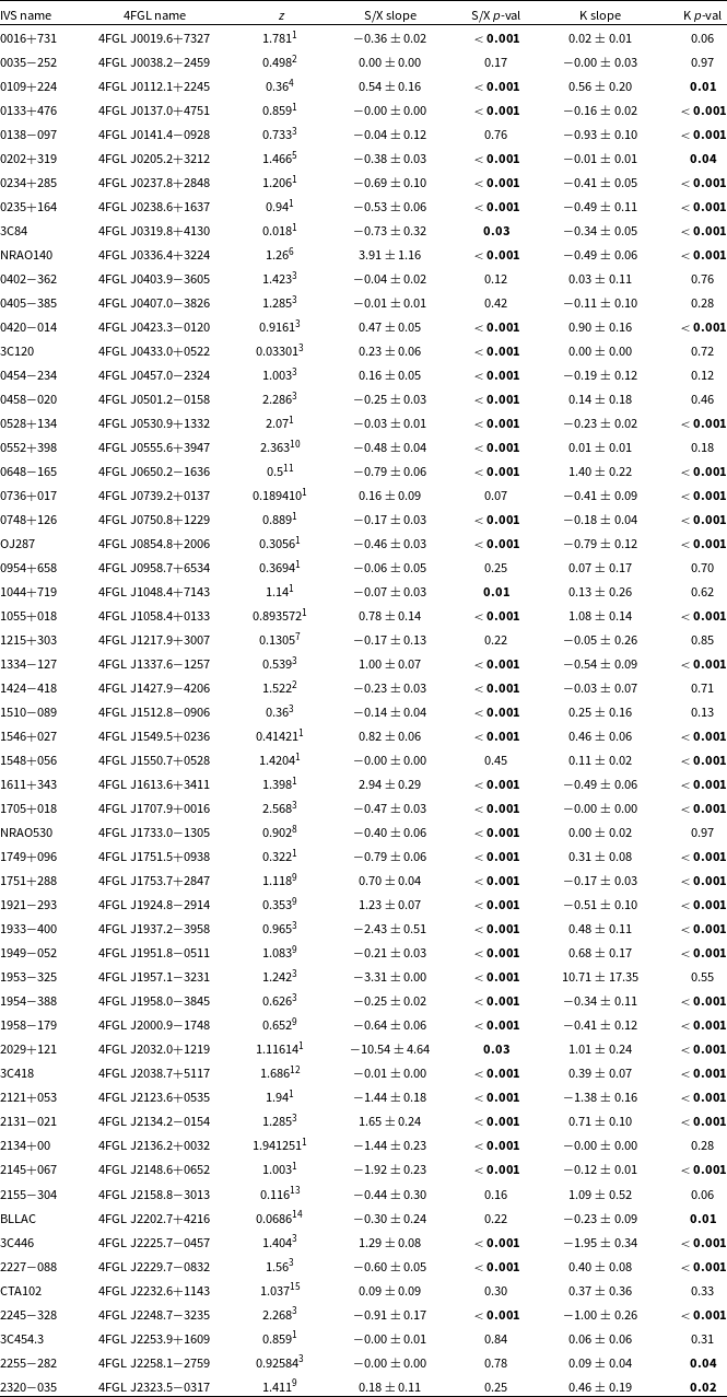
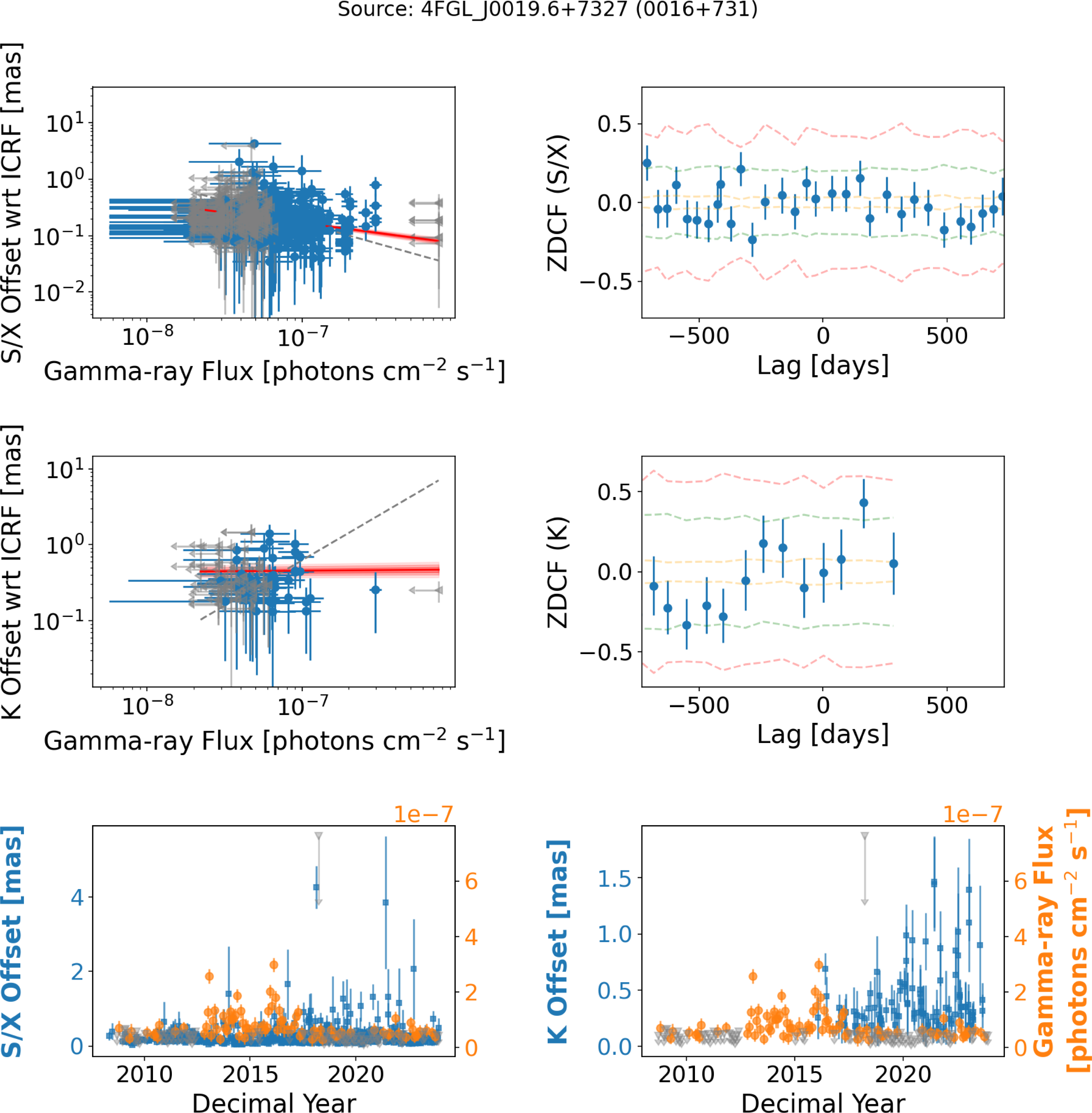
 σ
σ σ
σ σ
σ γ
γ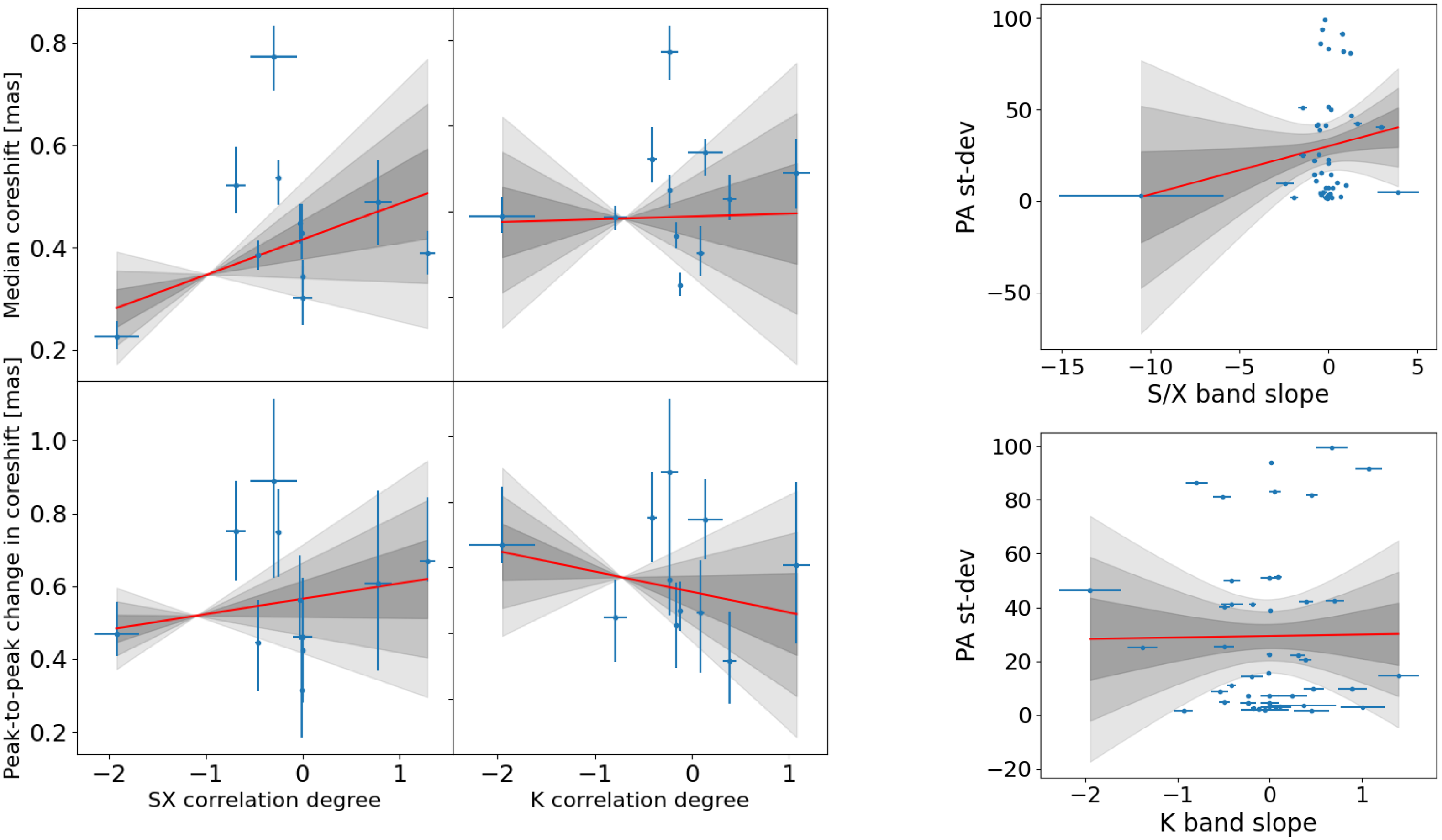
 σ
σ σ
σ σ
σ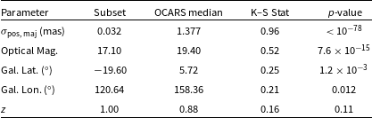
 N=92
N=92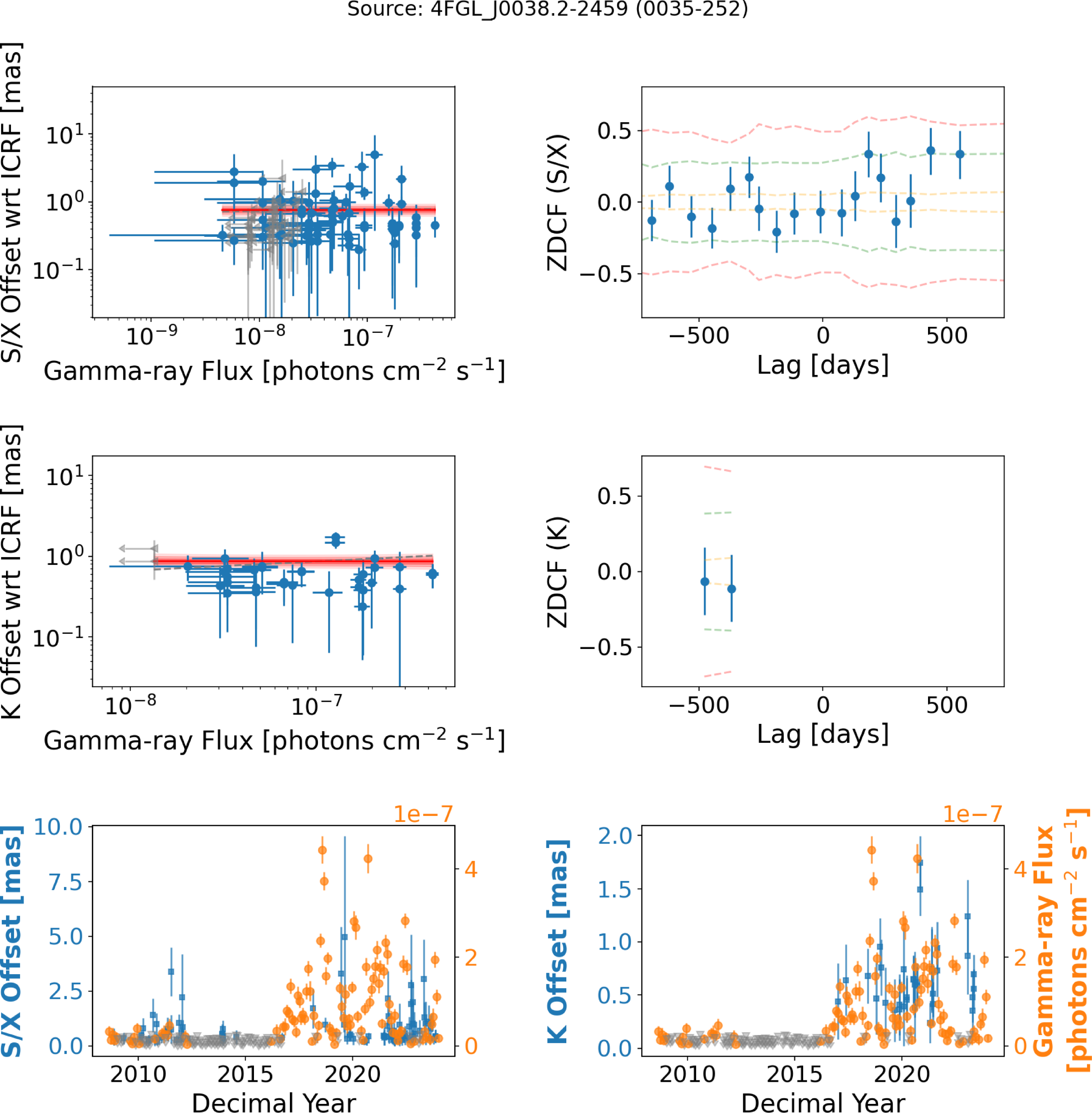
 −
−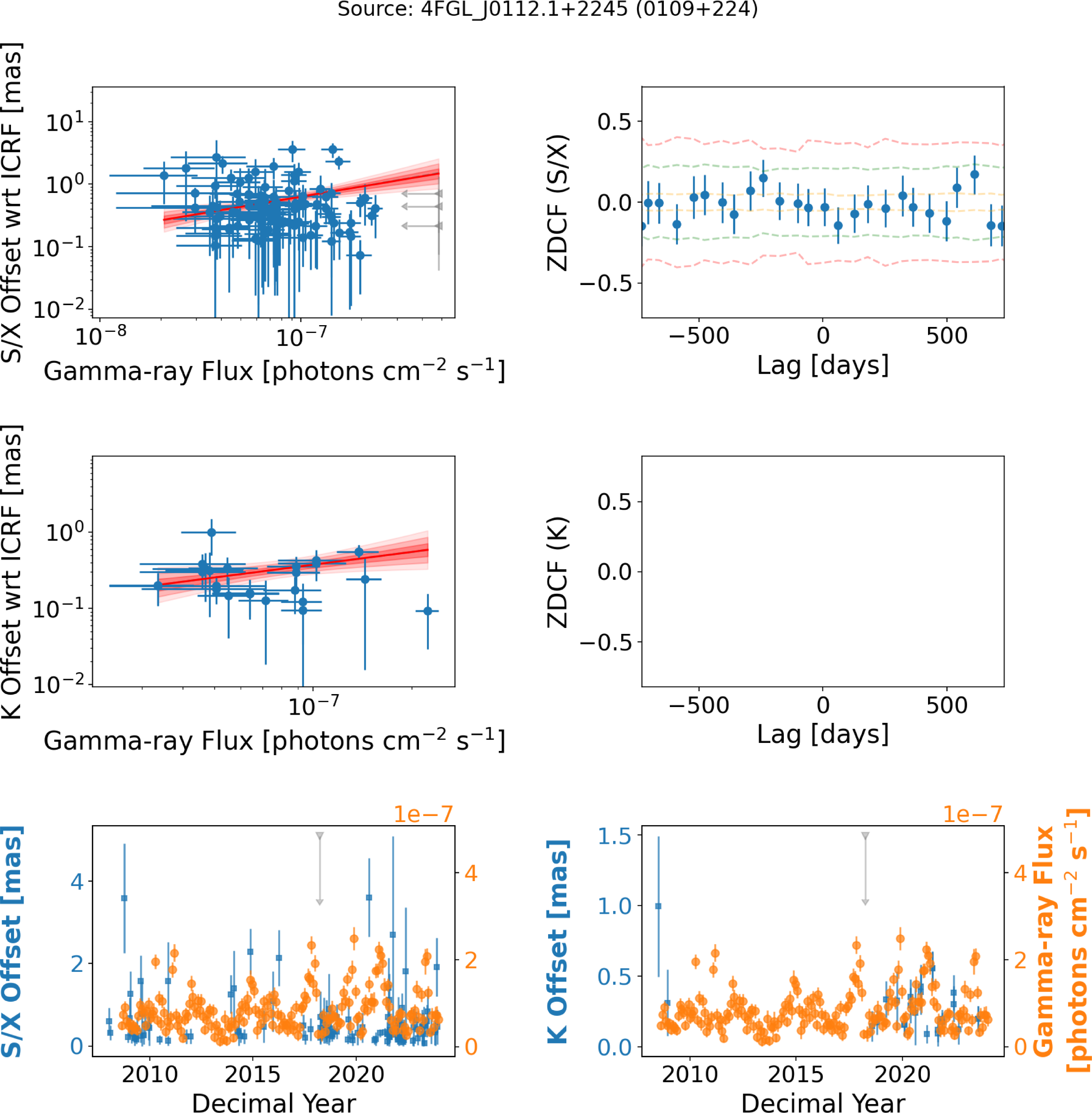
 +
+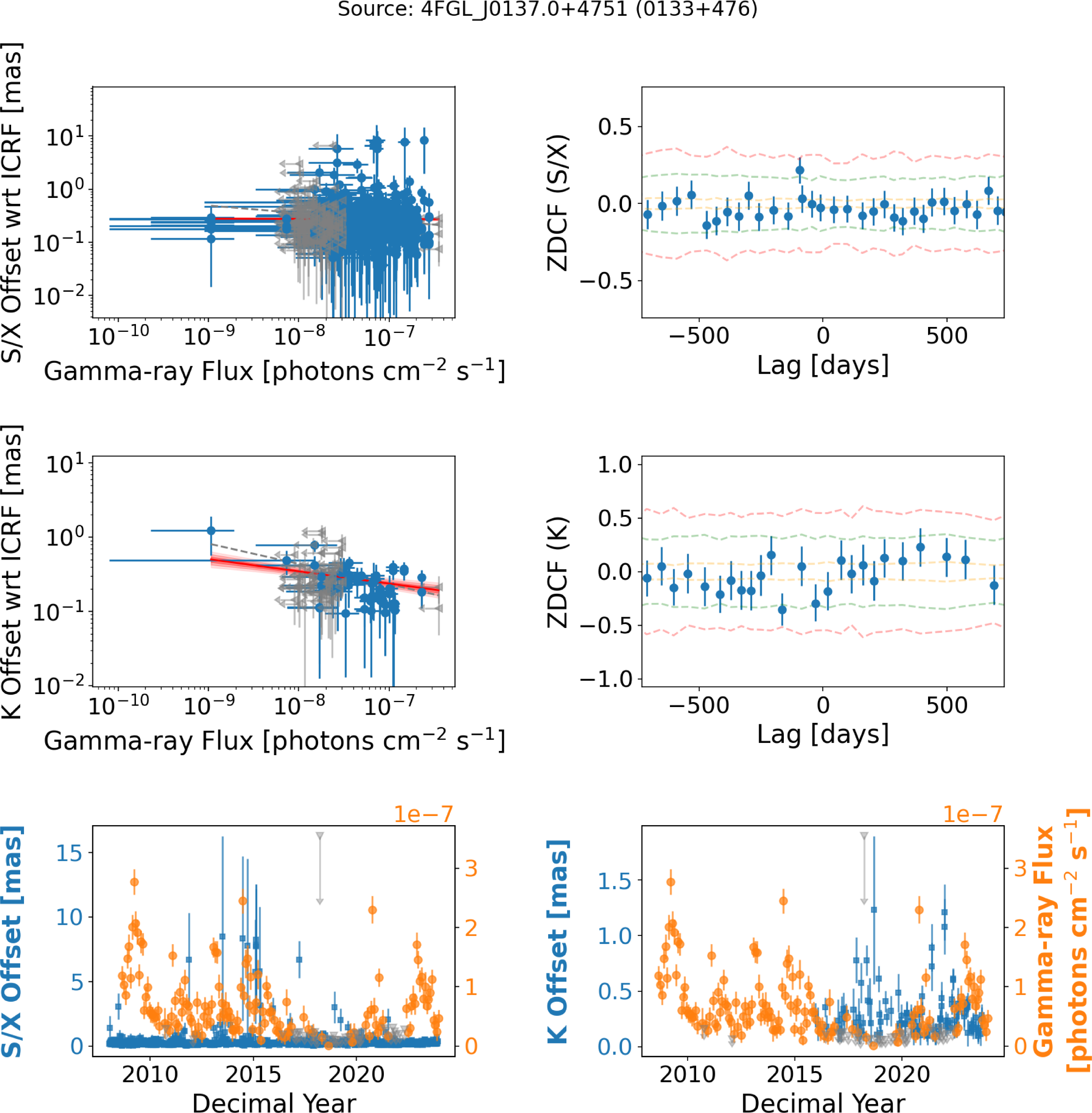
 +
+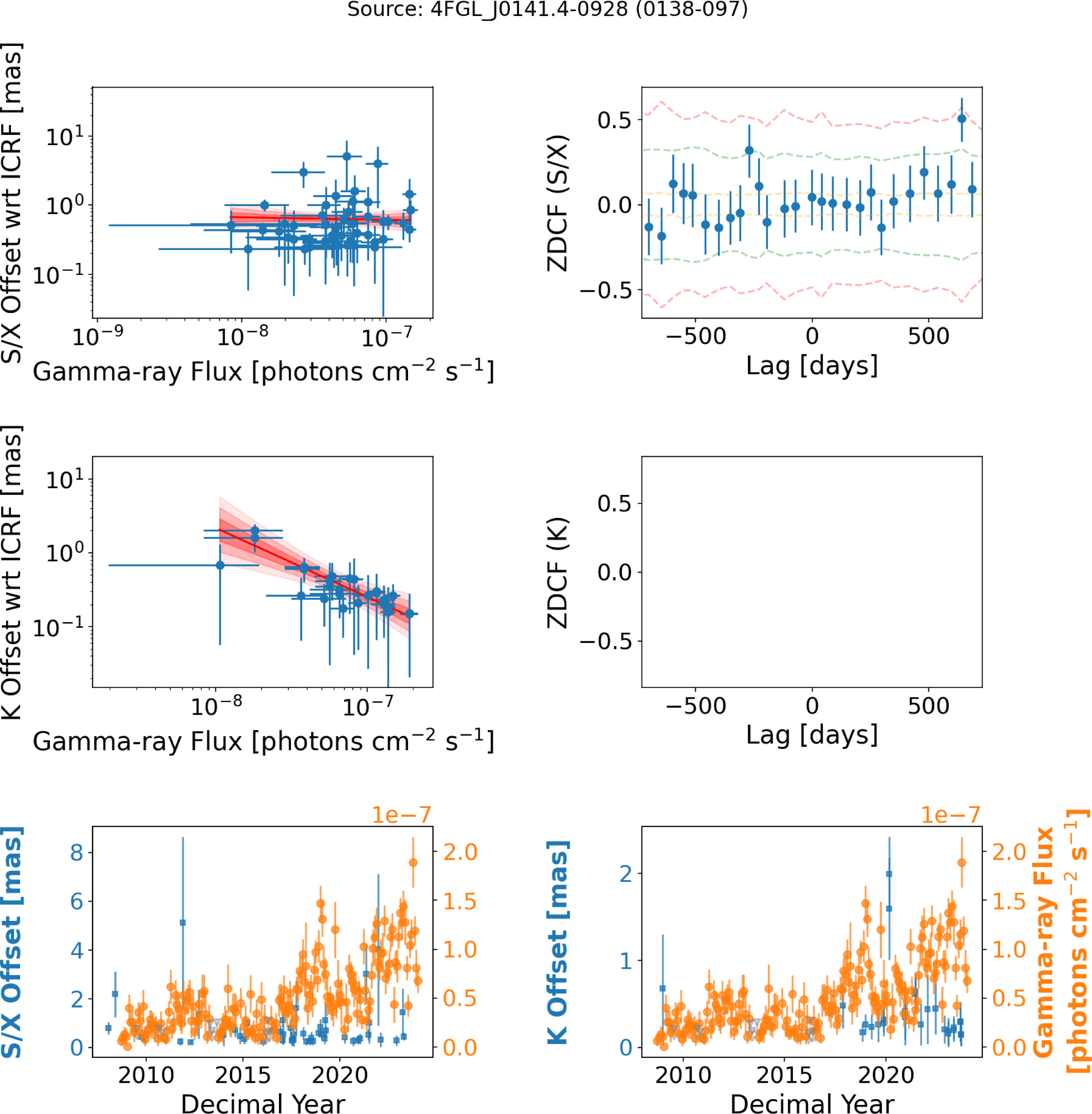
 −
−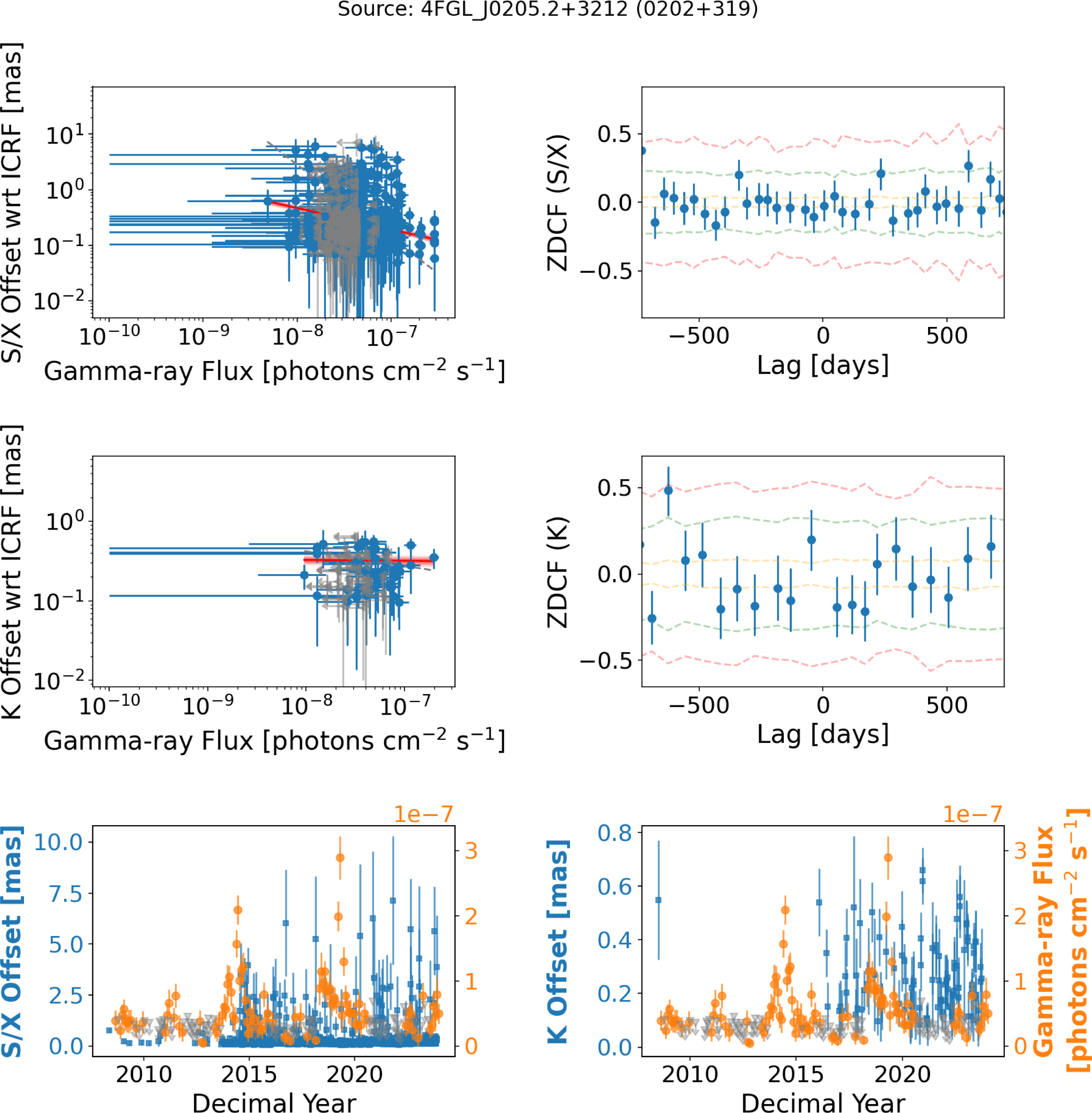
 +
+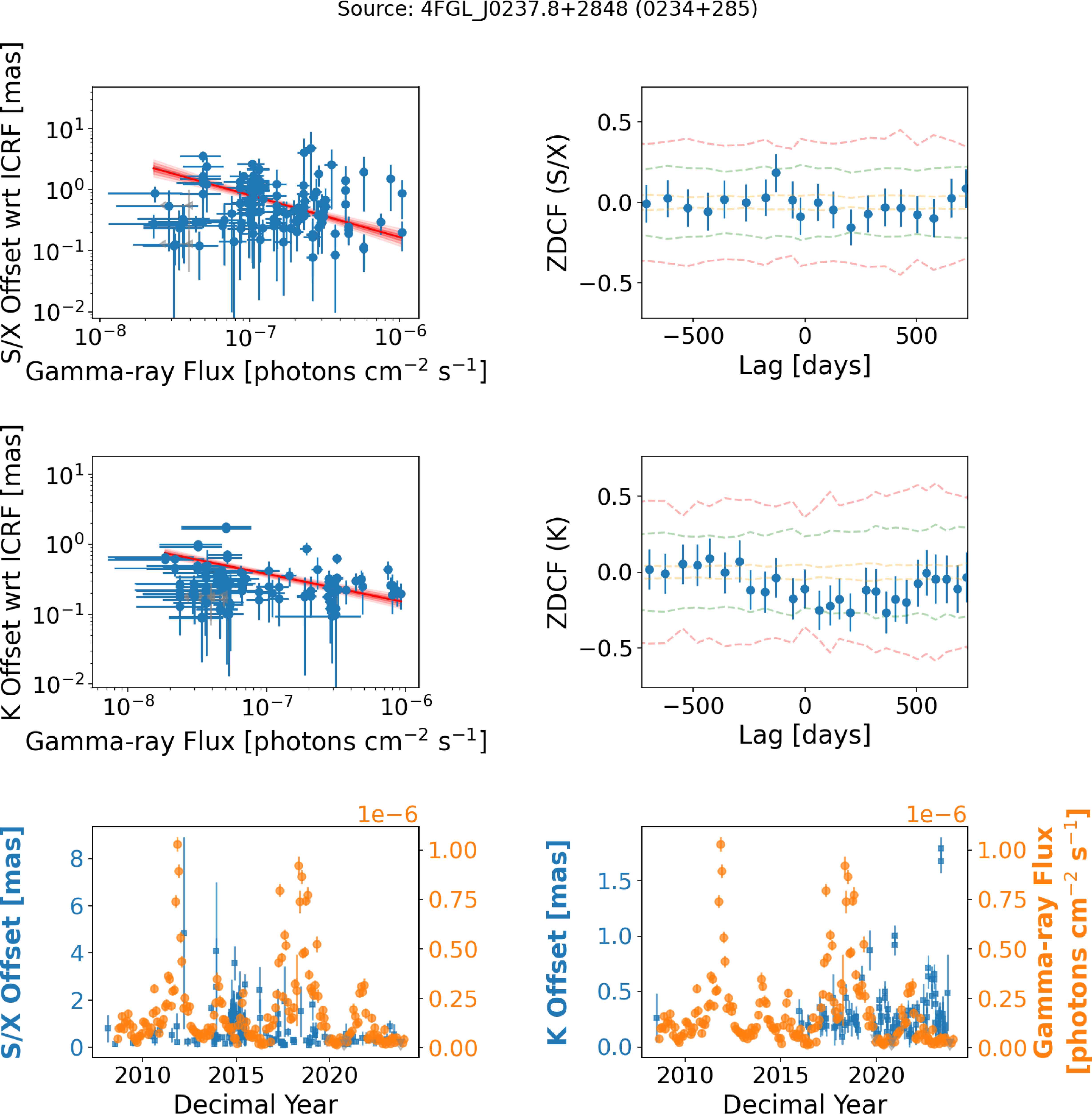
 +
+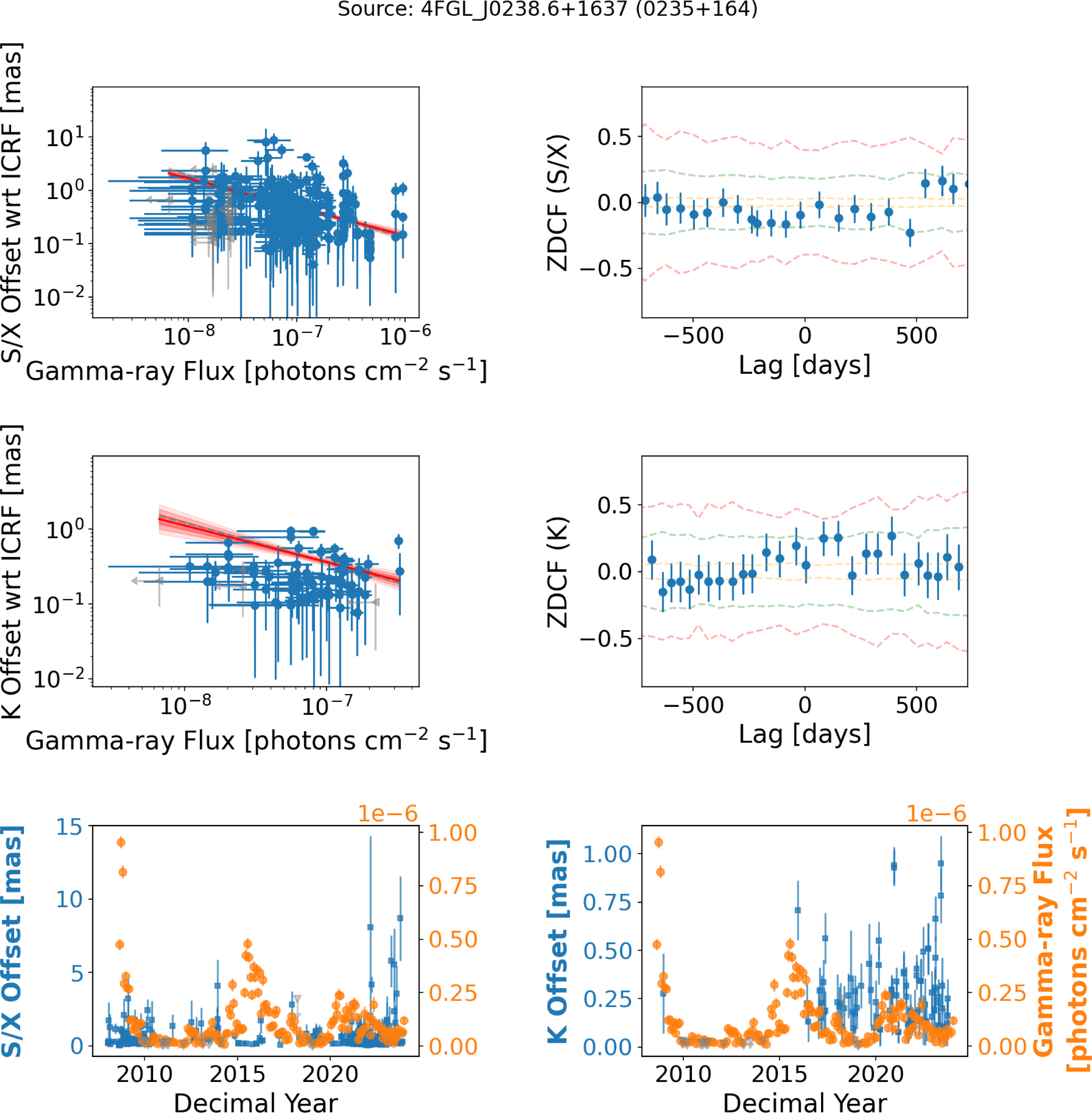
 +
+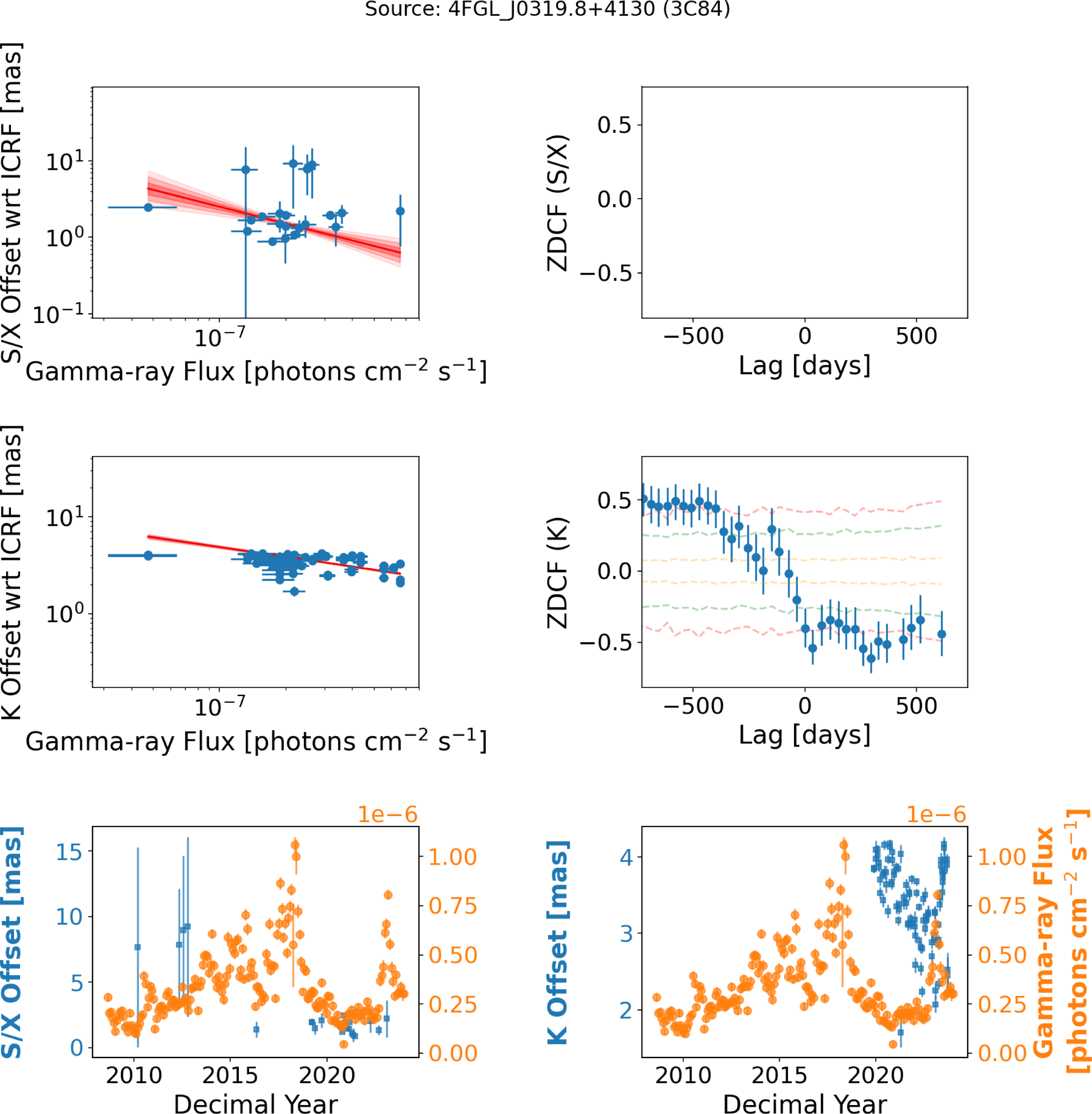
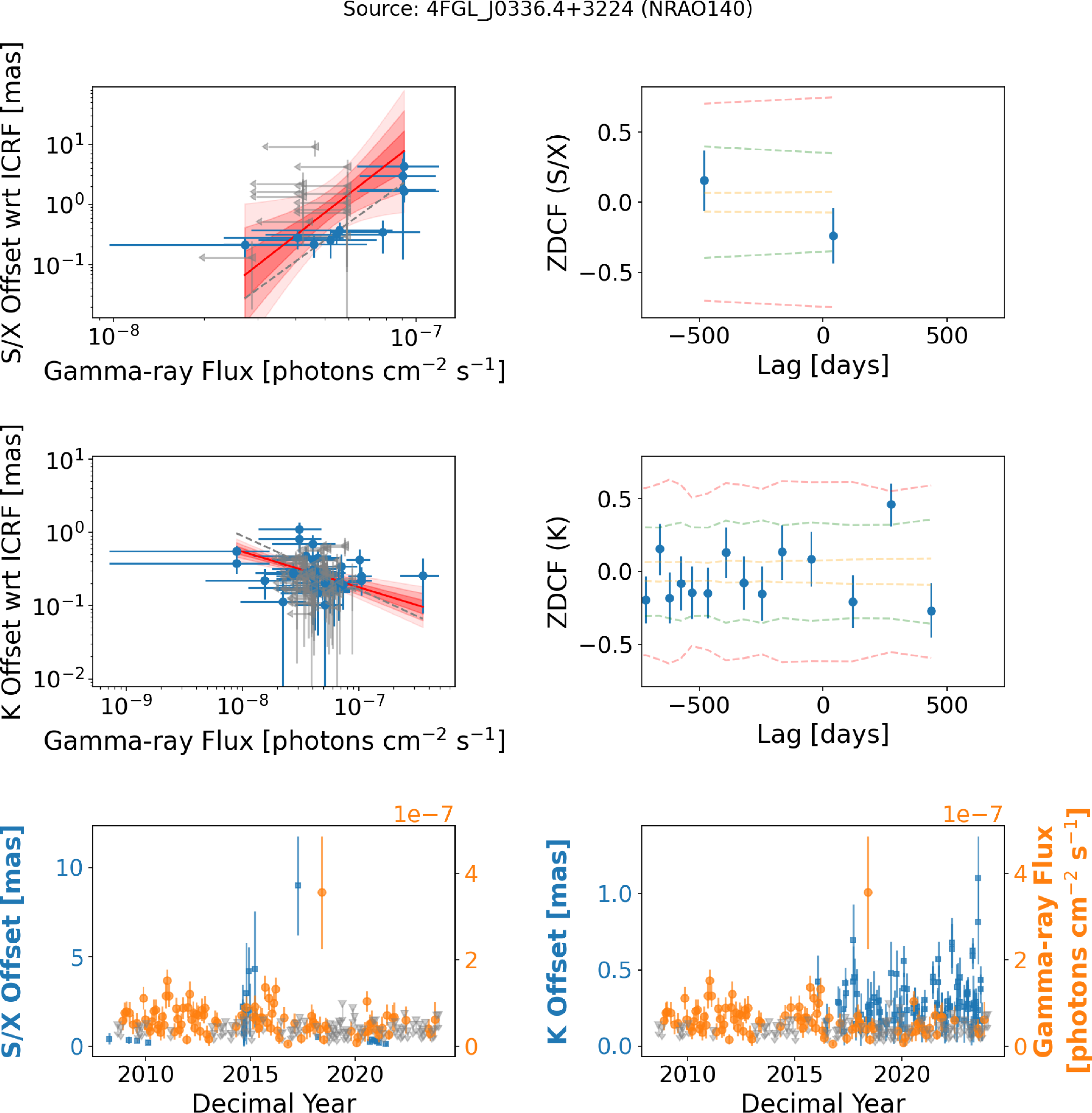
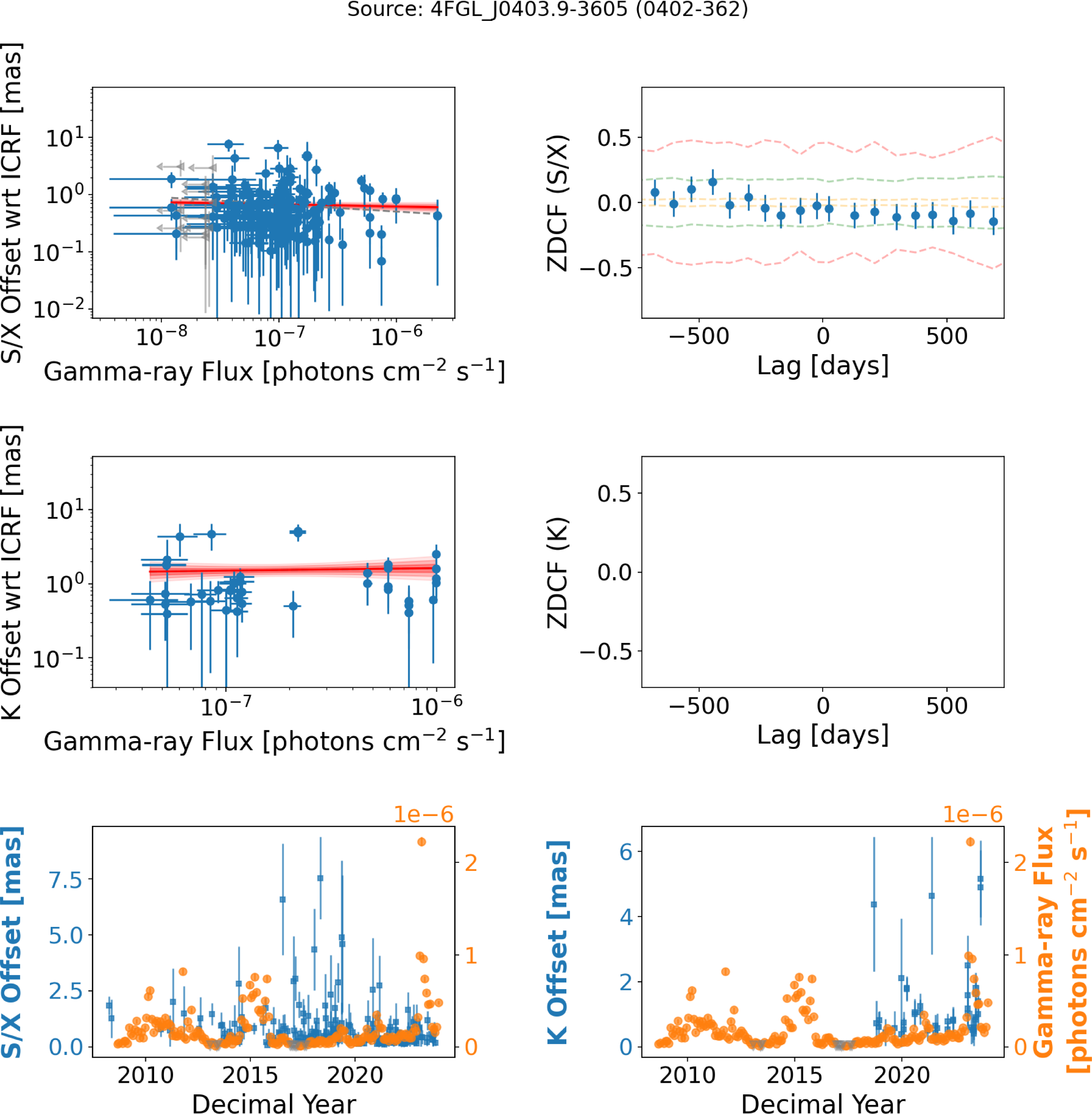
 −
−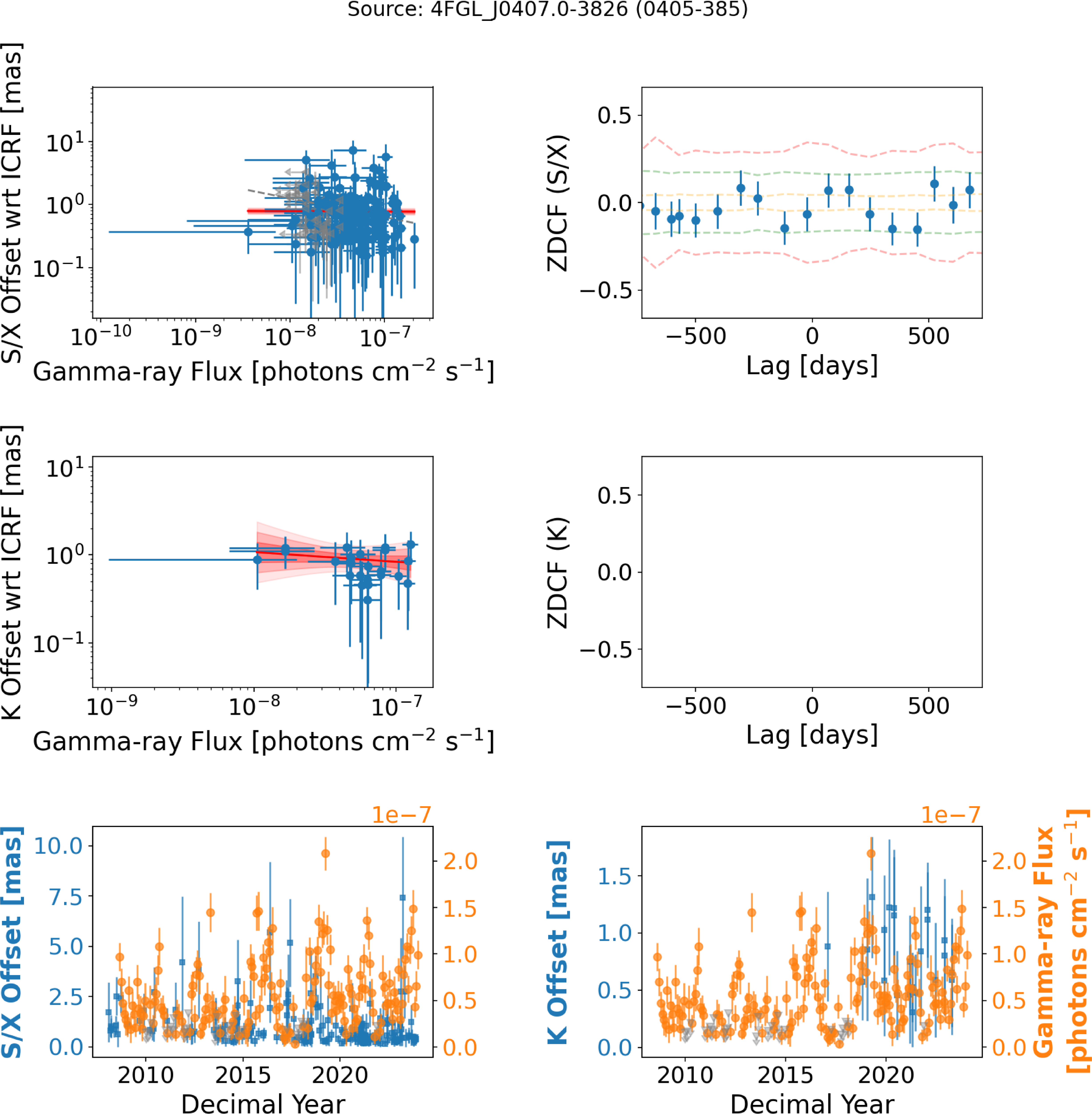
 −
−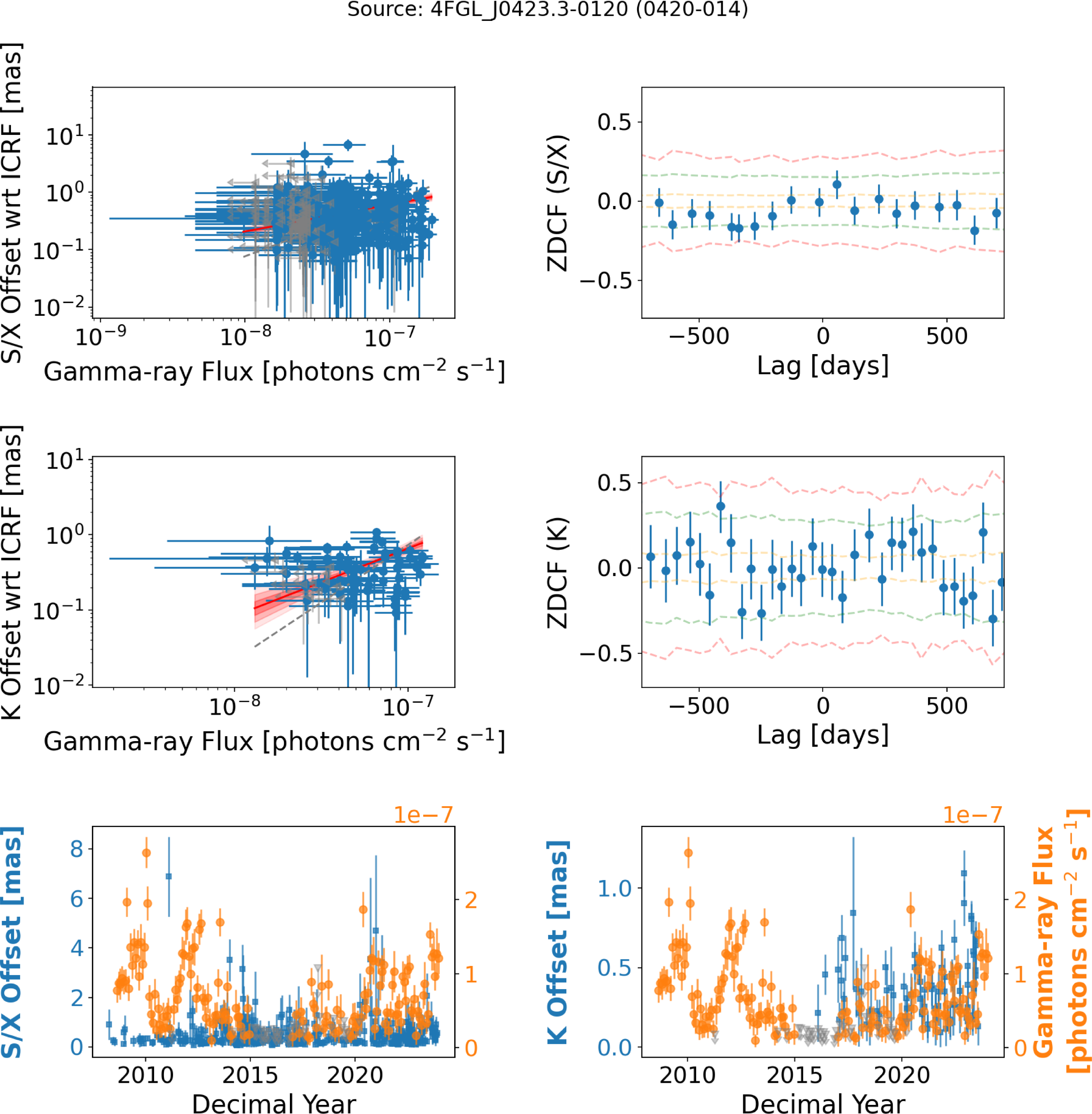
 −
−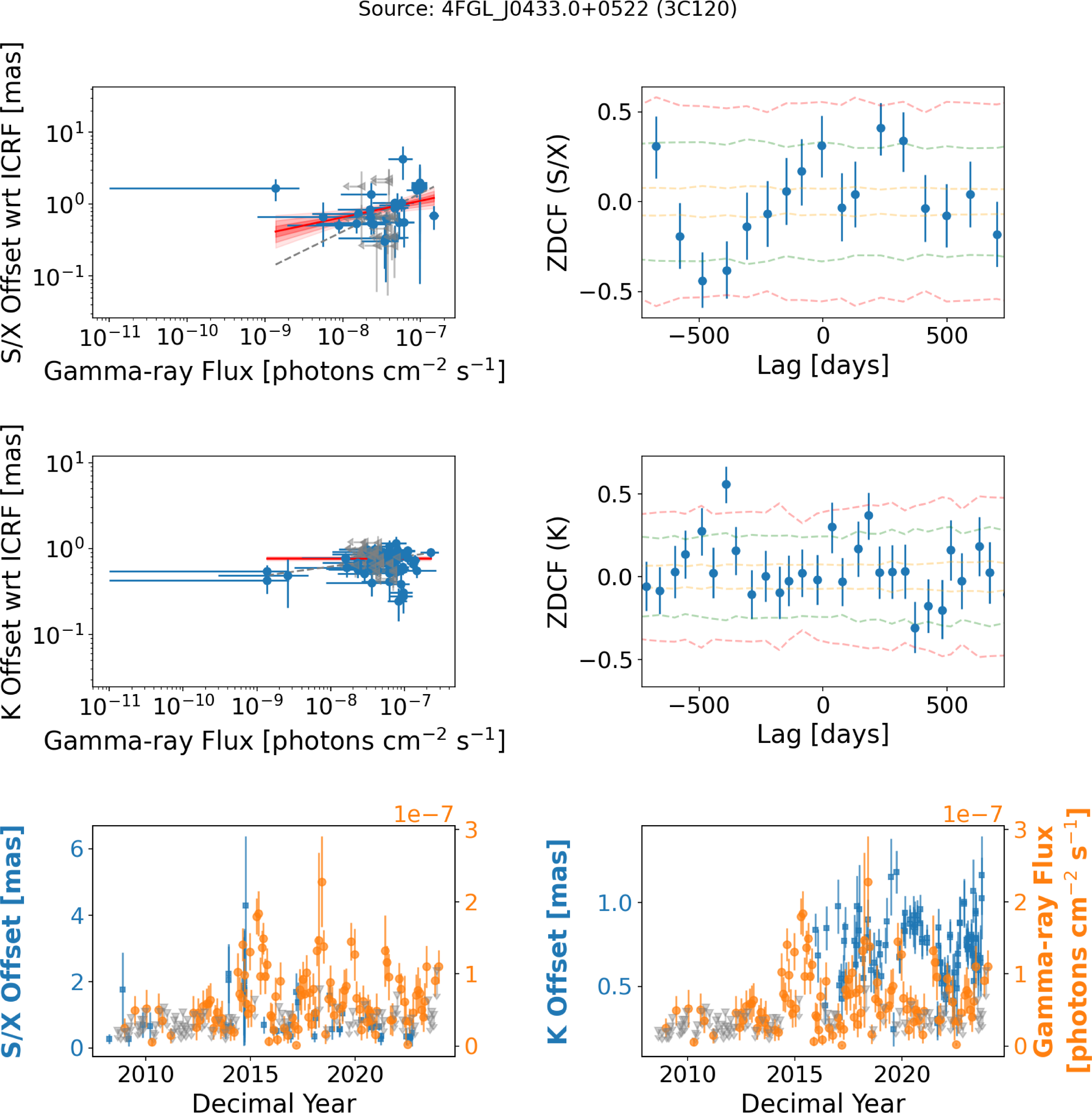
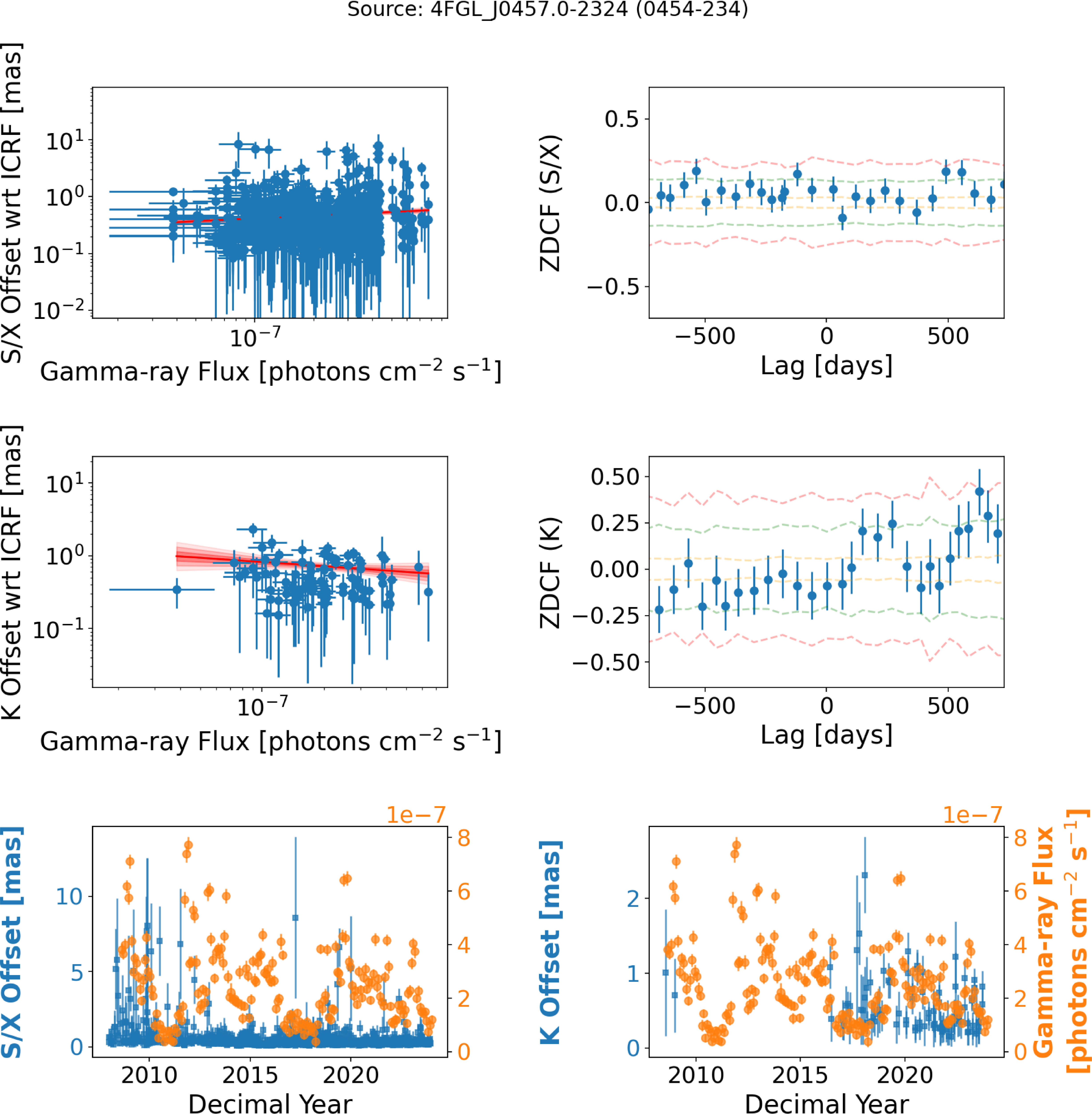
 −
−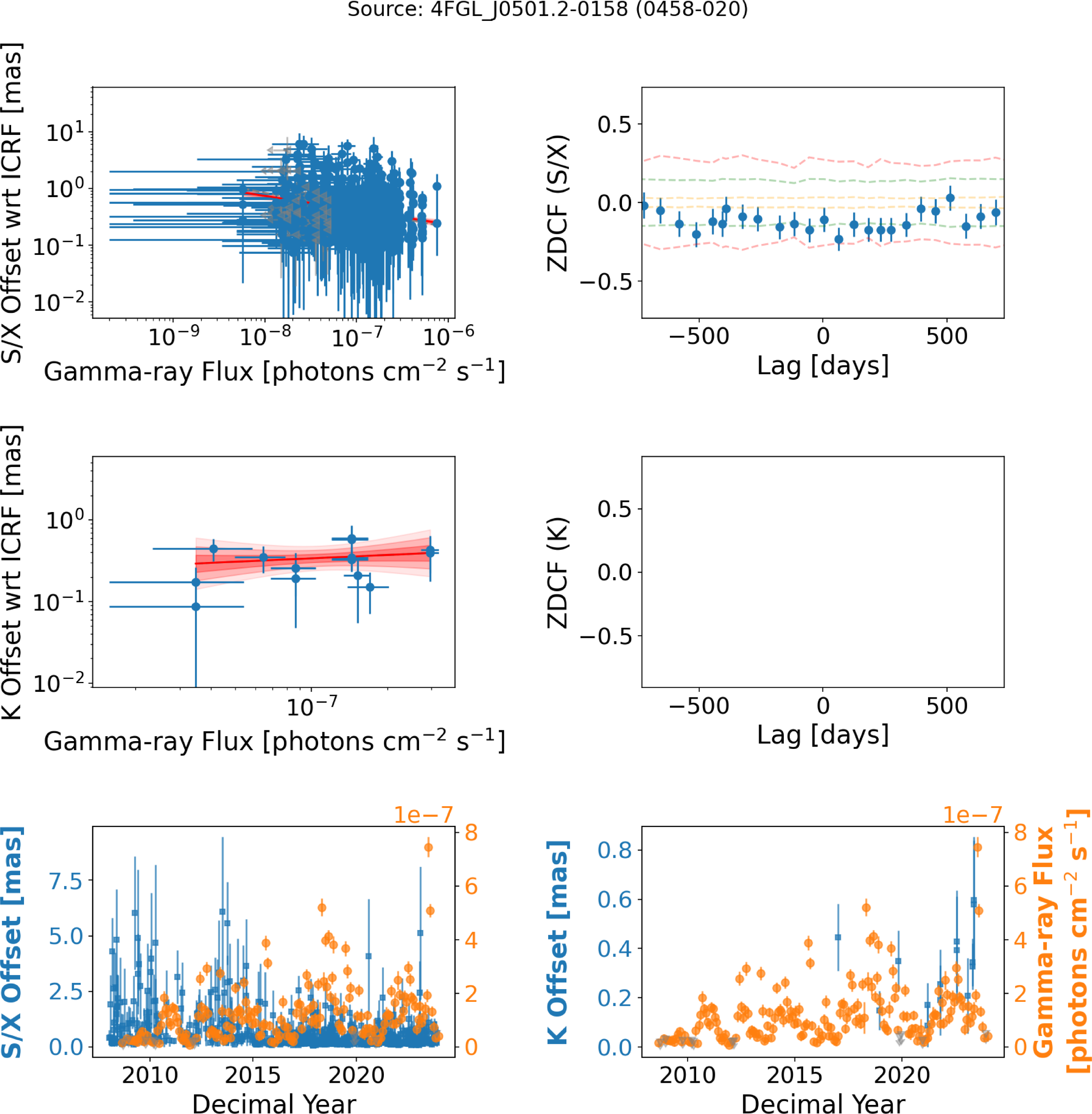
 −
−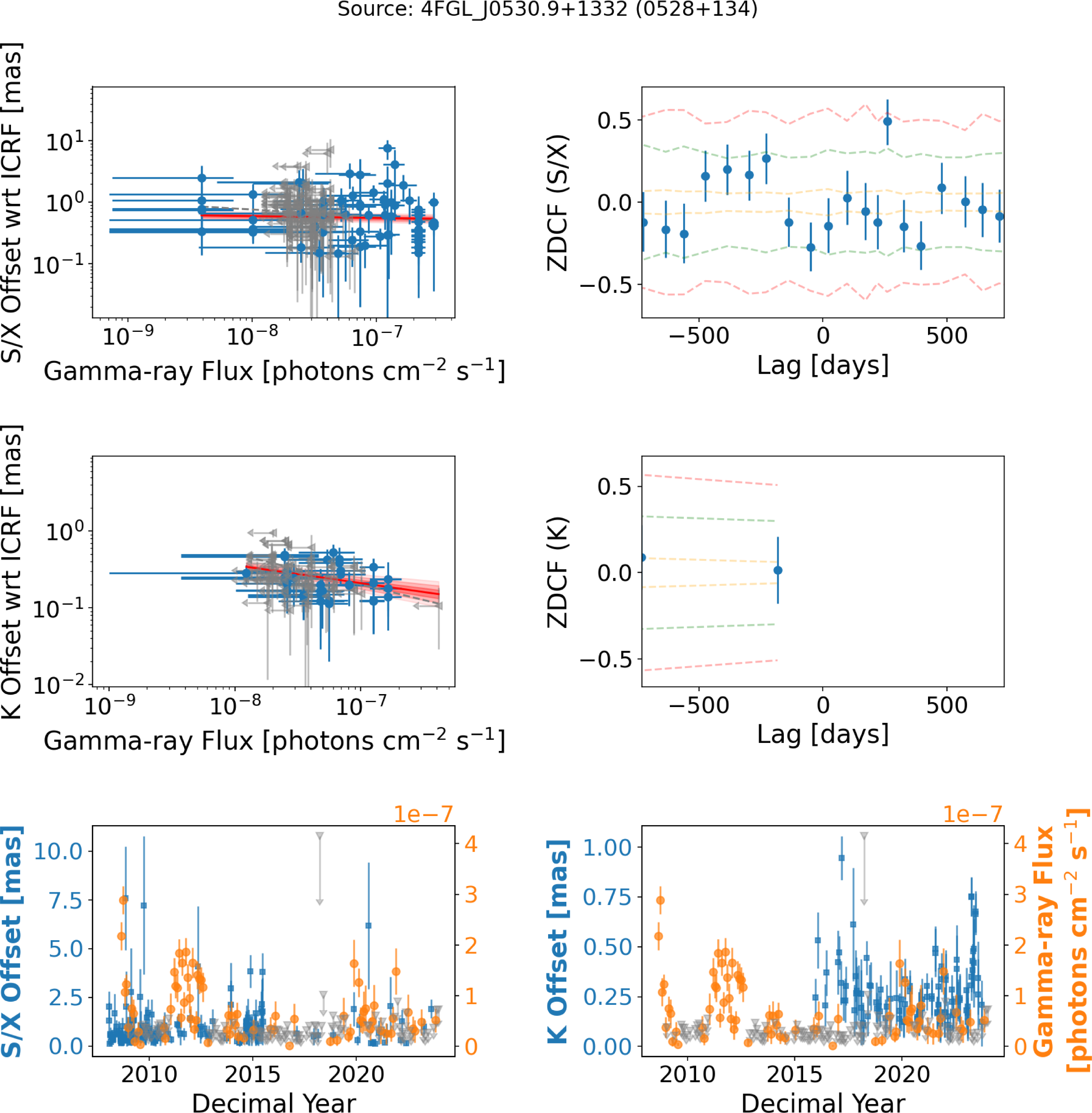
 +
+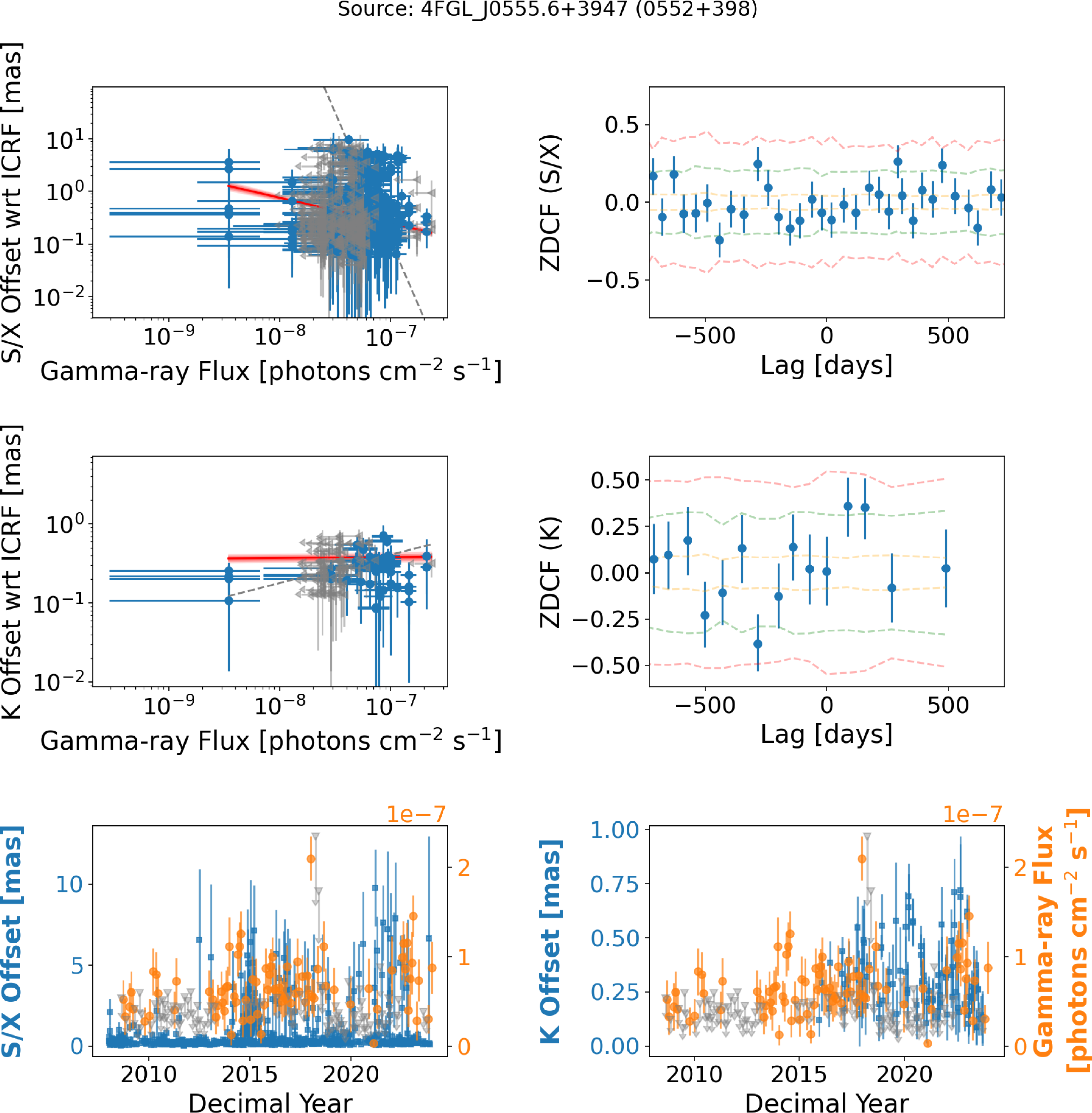
 +
+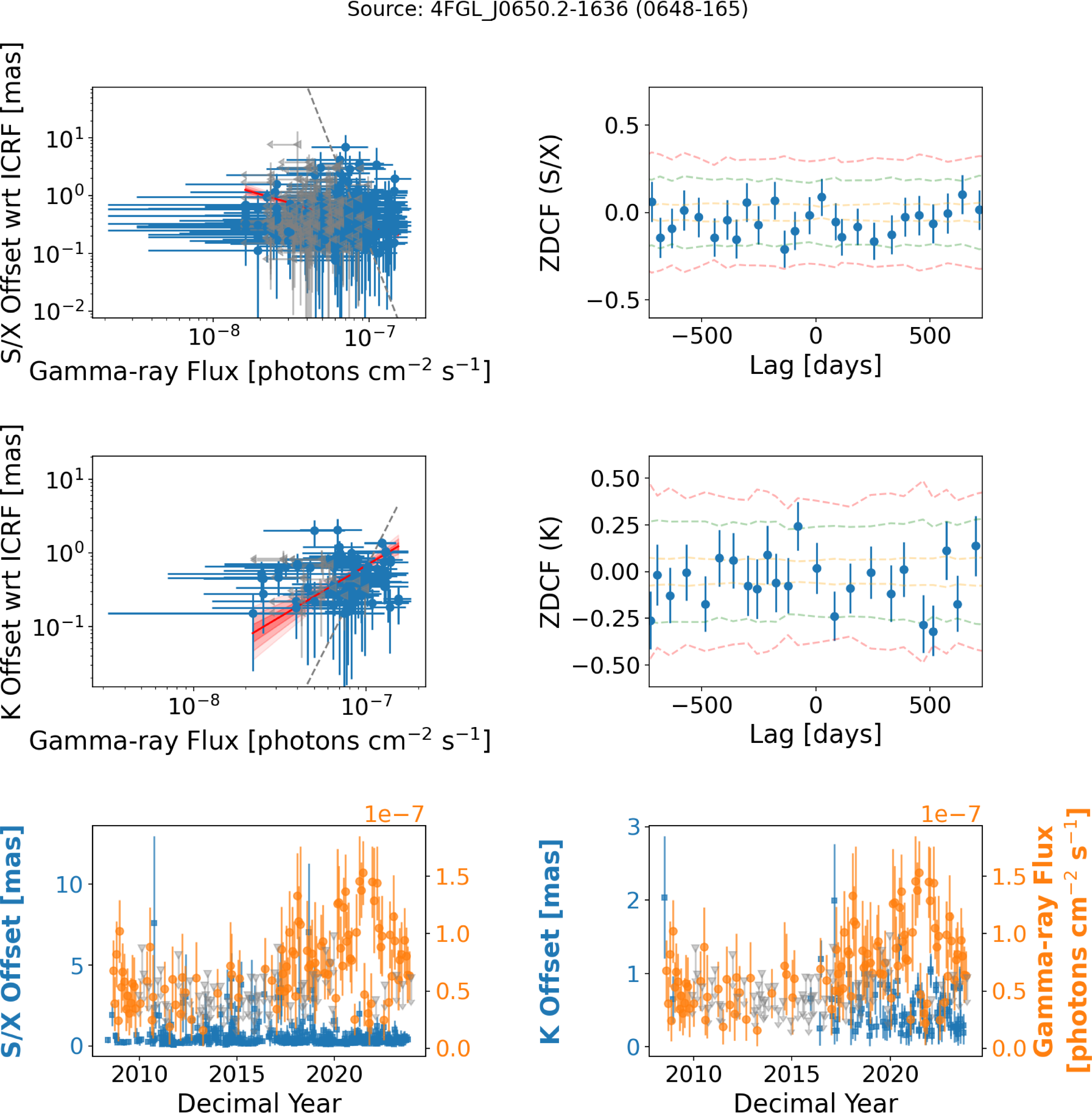
 −
−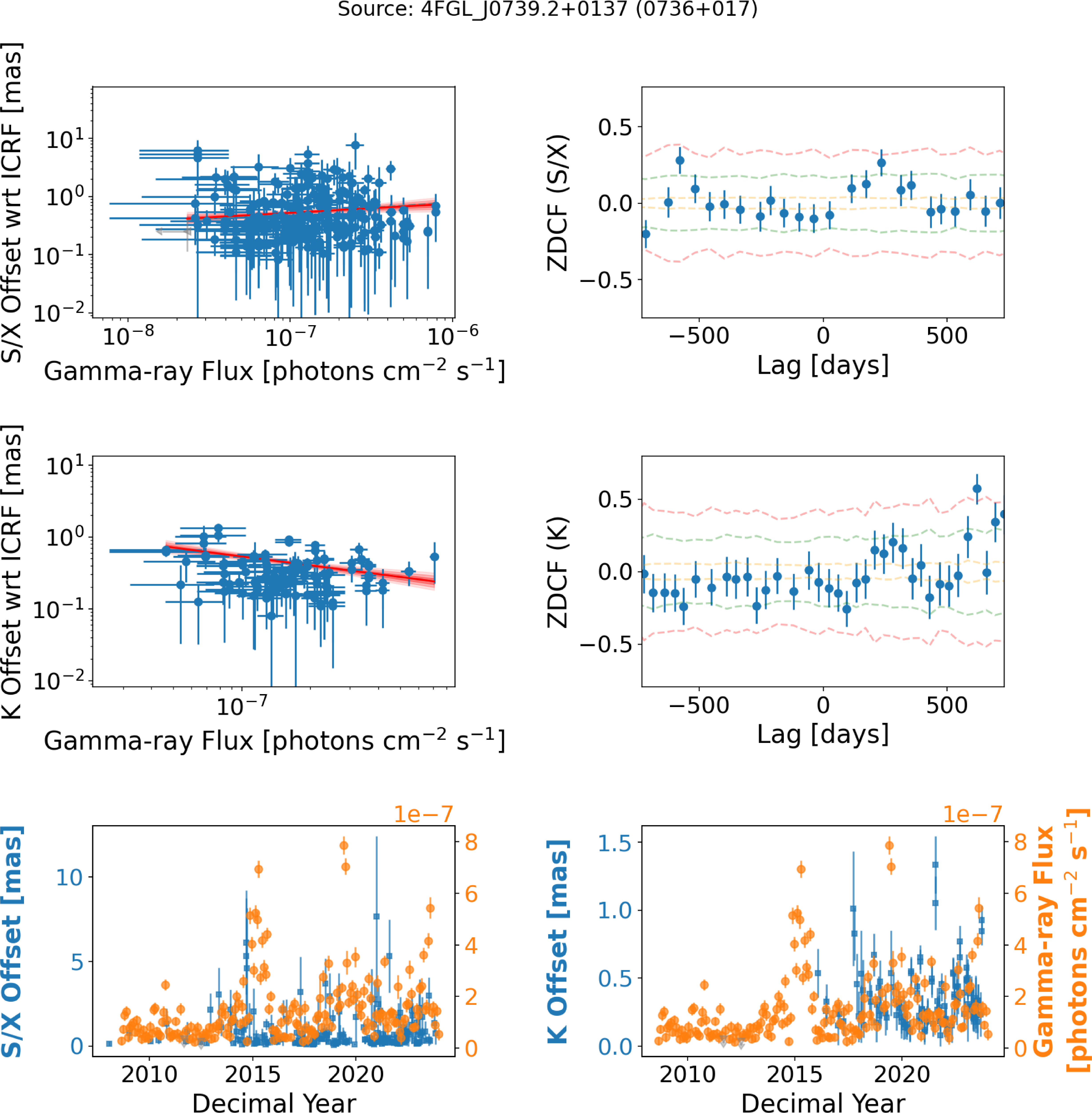
 +
+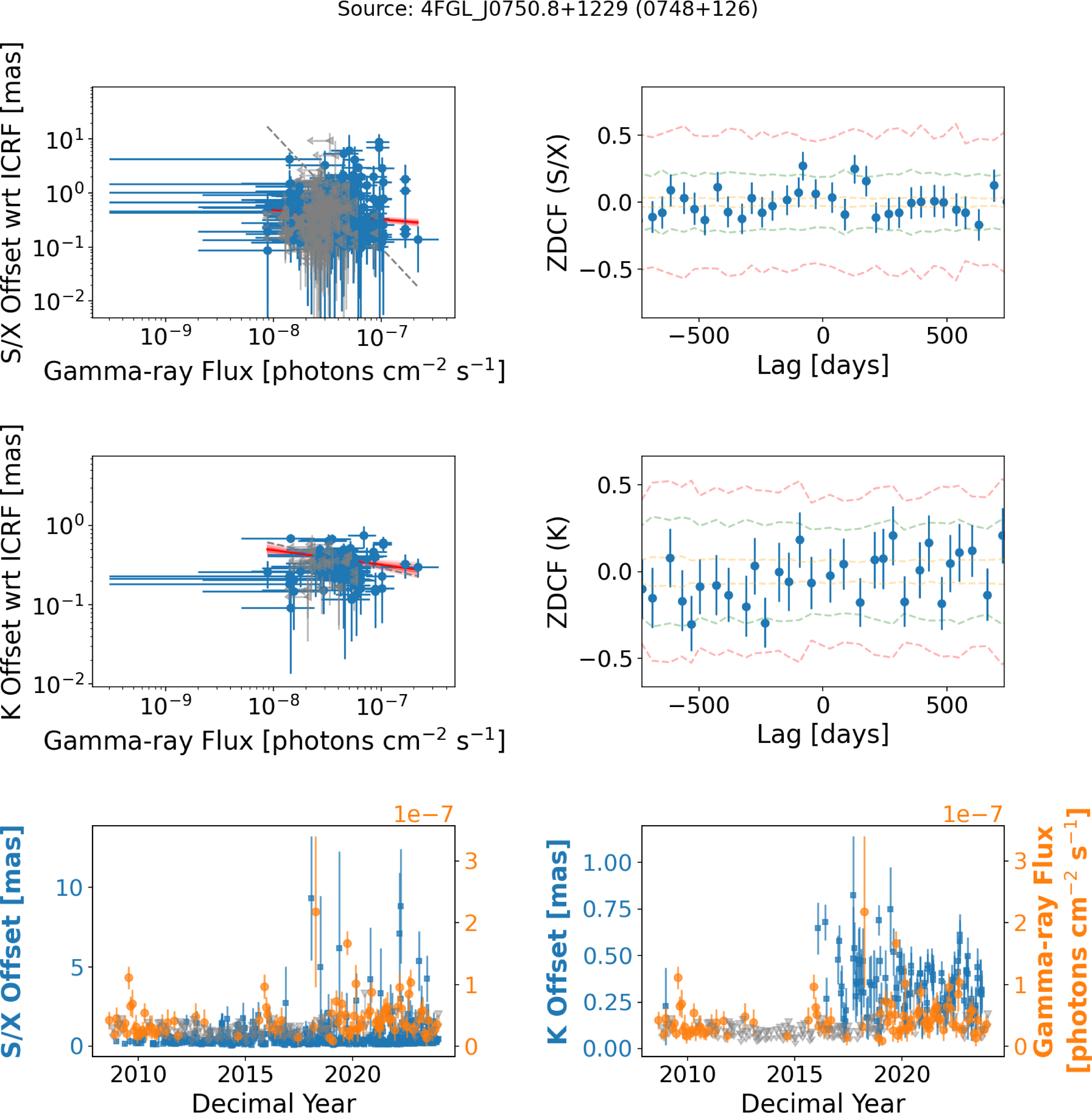
 +
+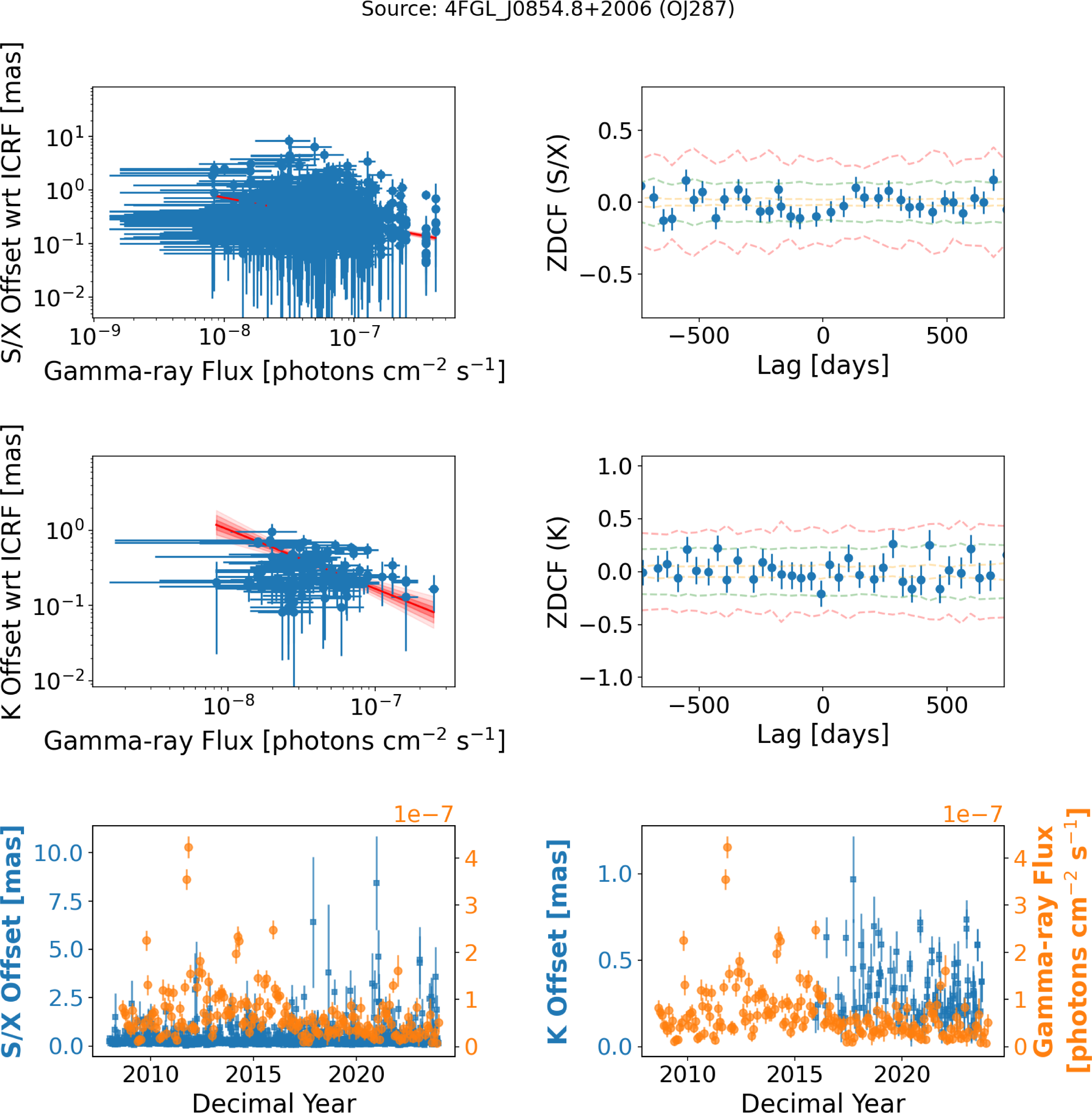
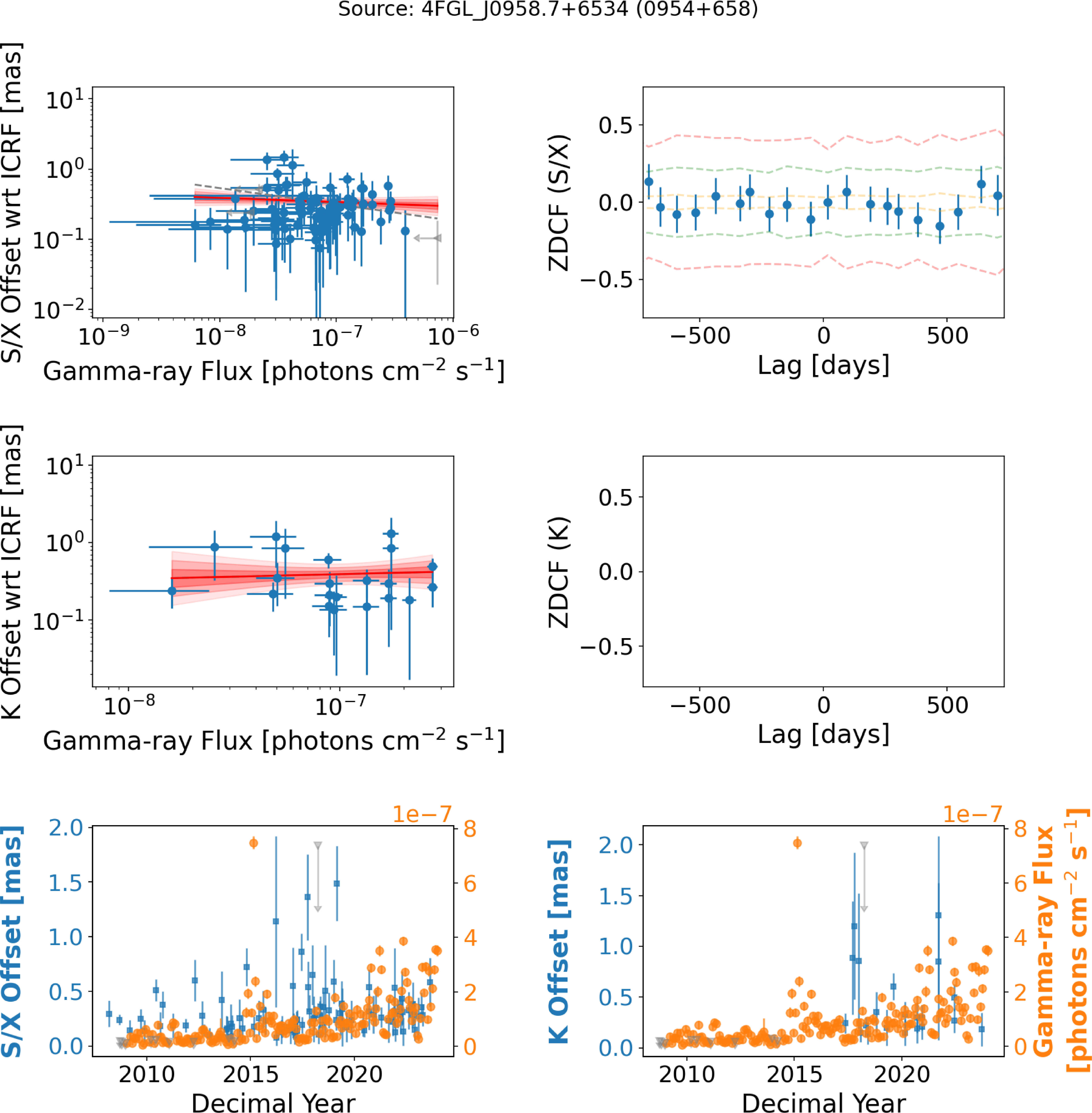
 +
+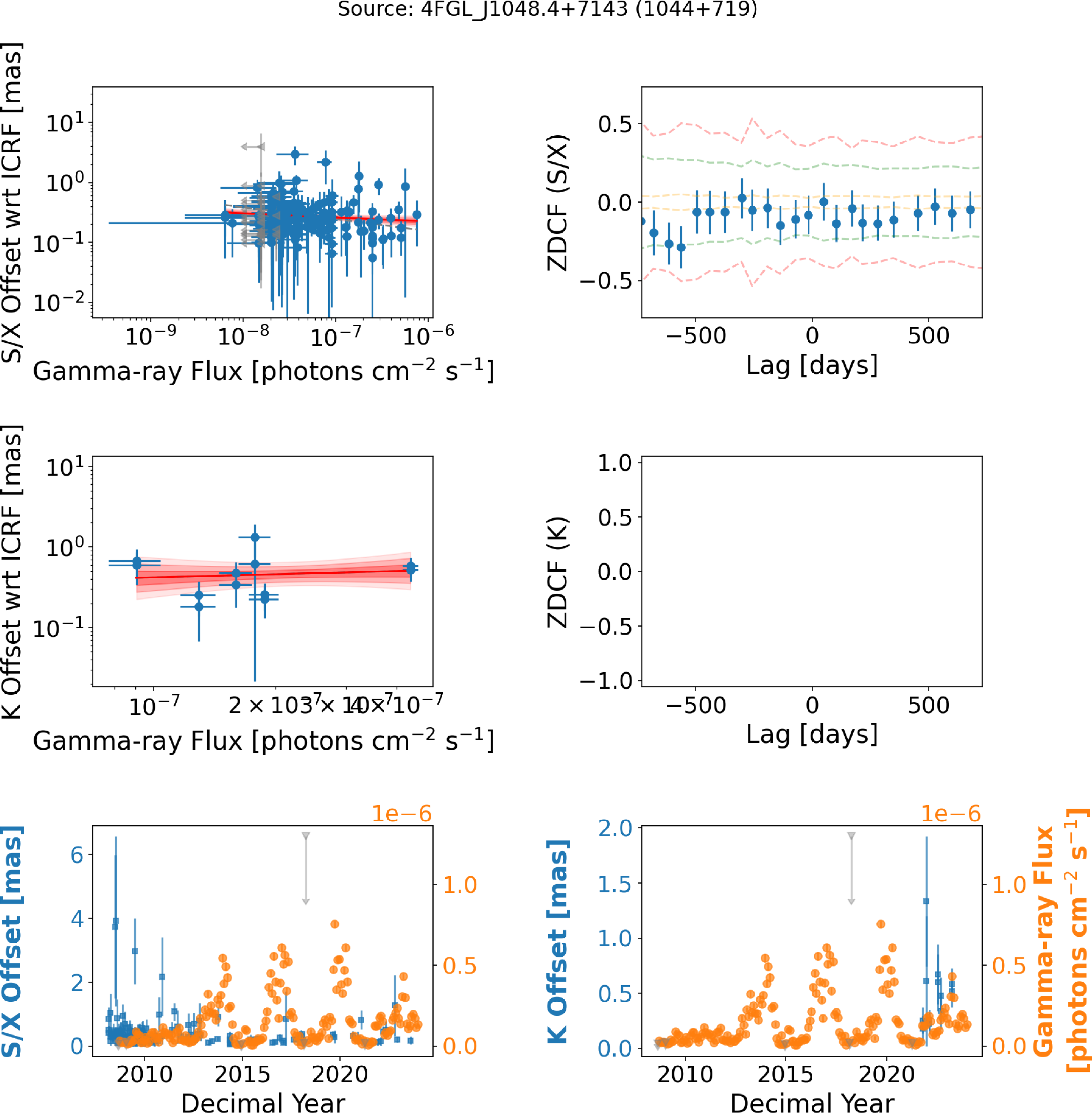
 +
+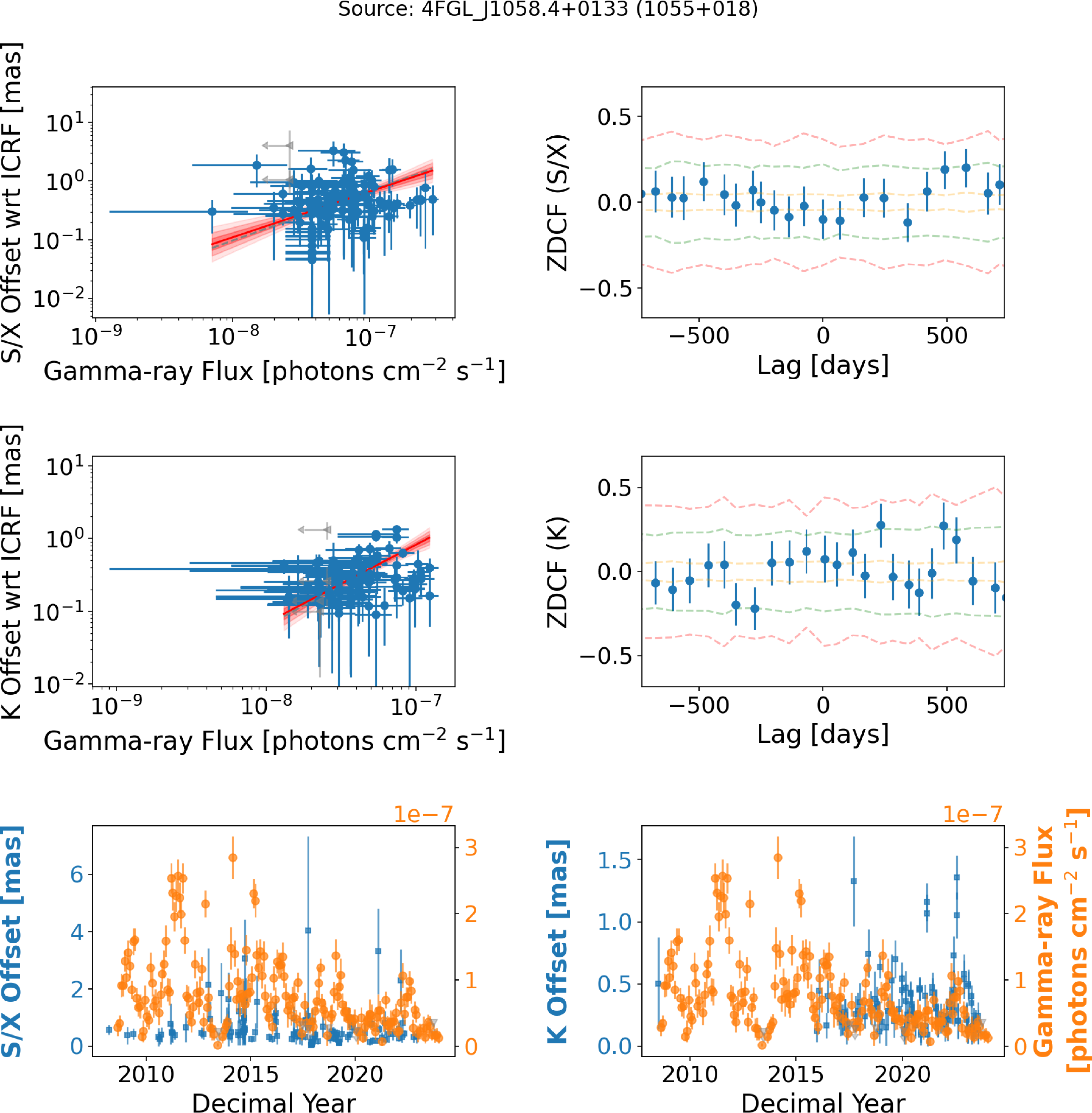
 +
+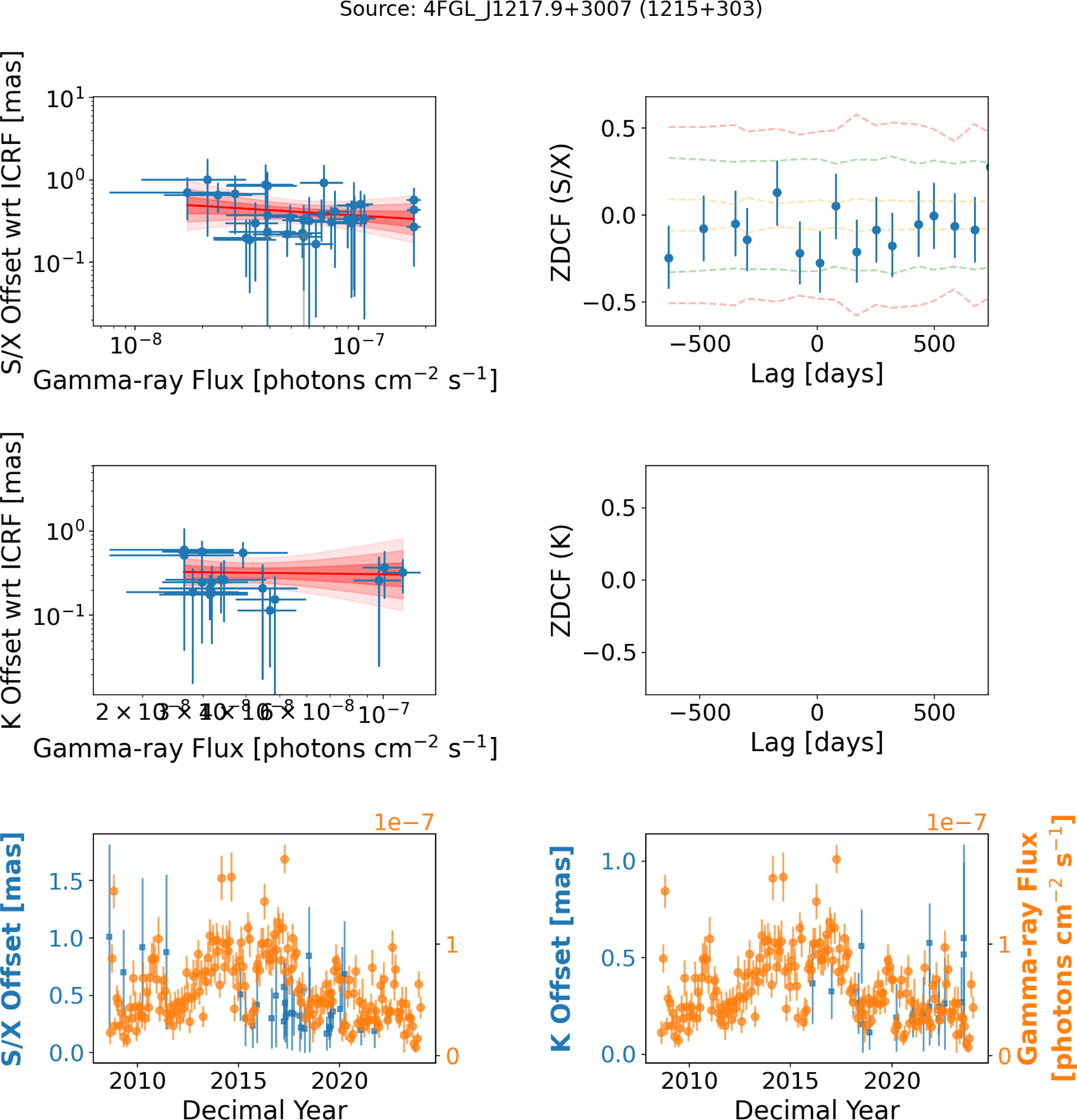
 +
+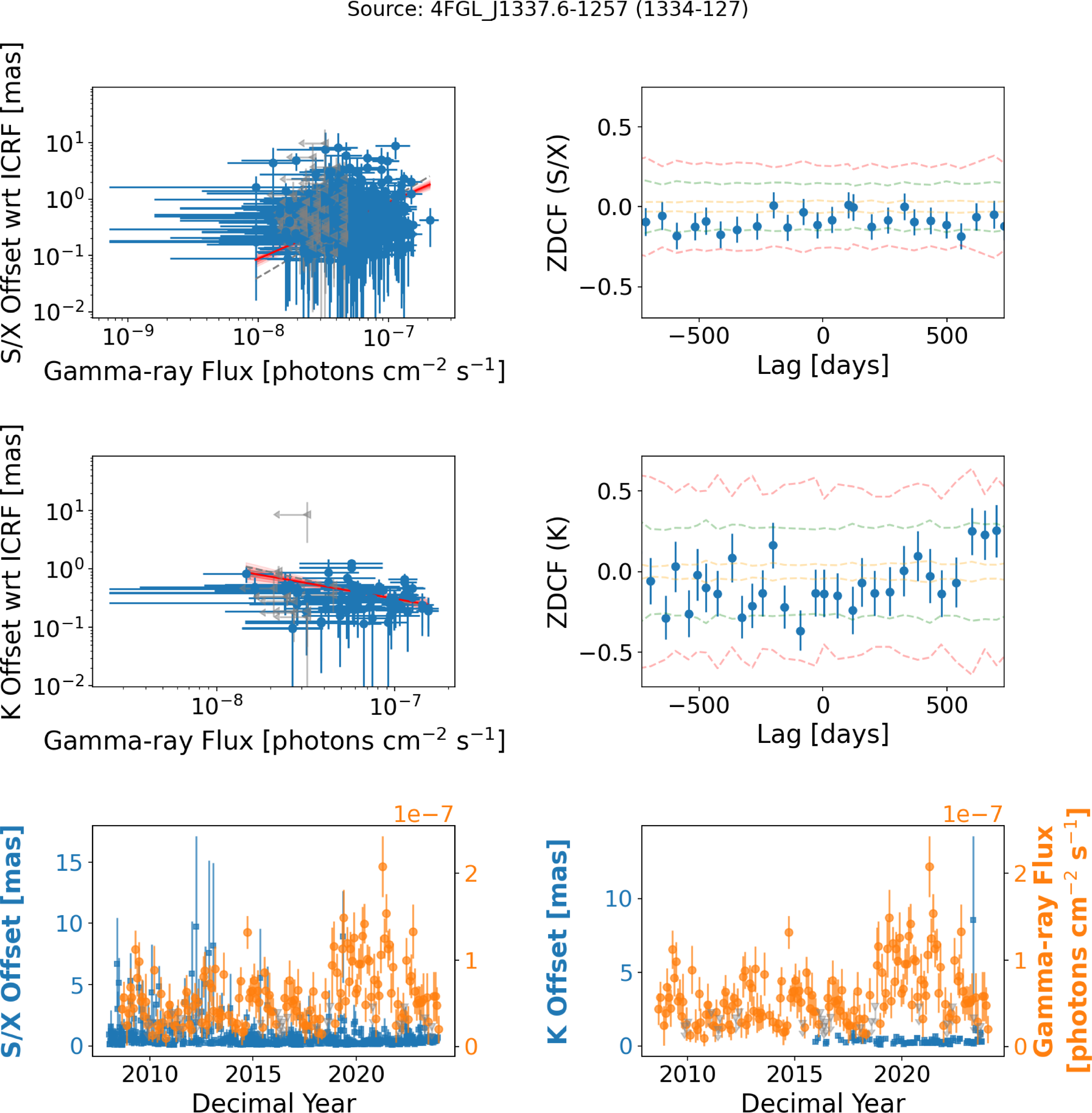
 −
−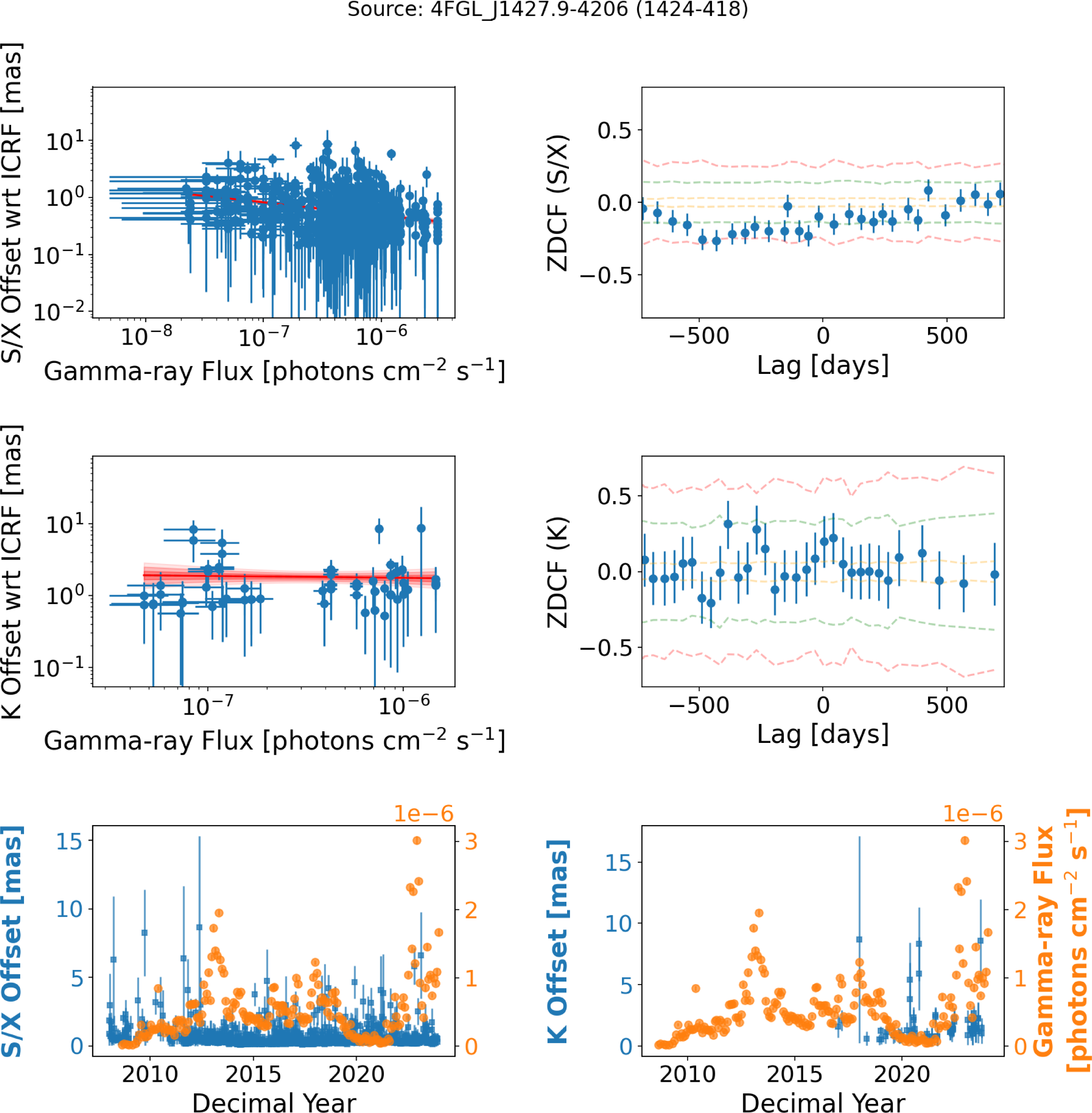
 −
−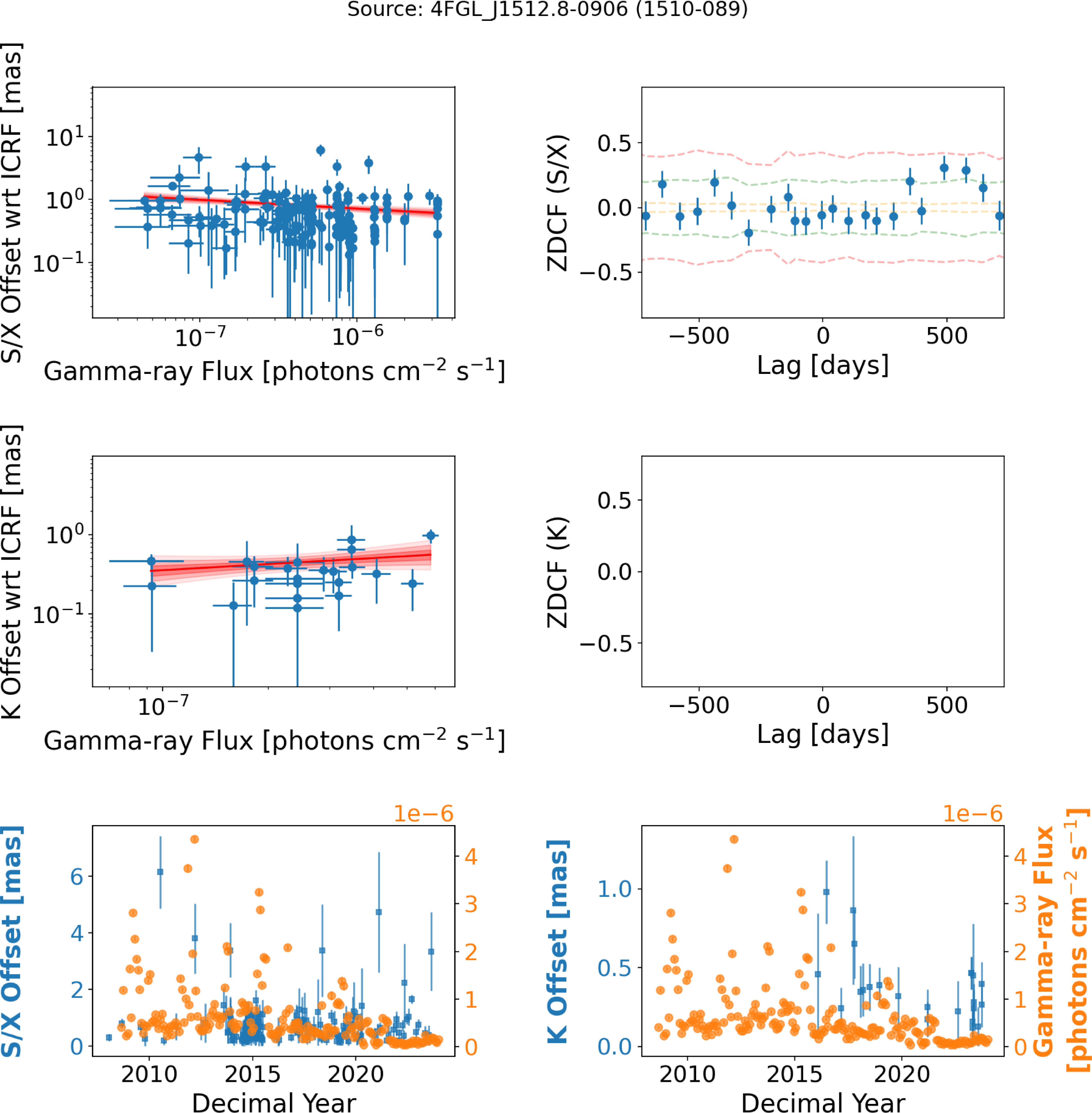
 −
−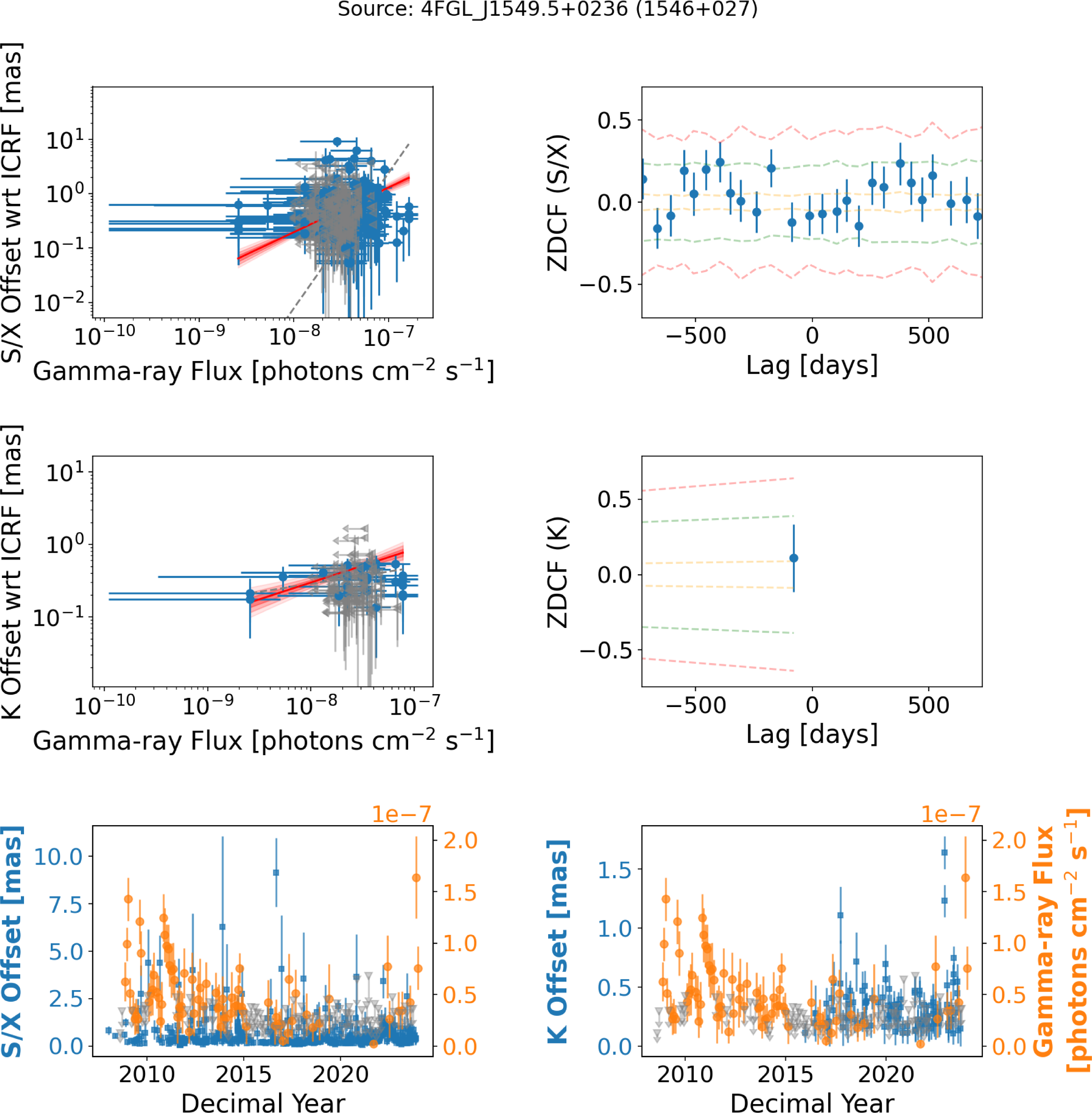
 +
+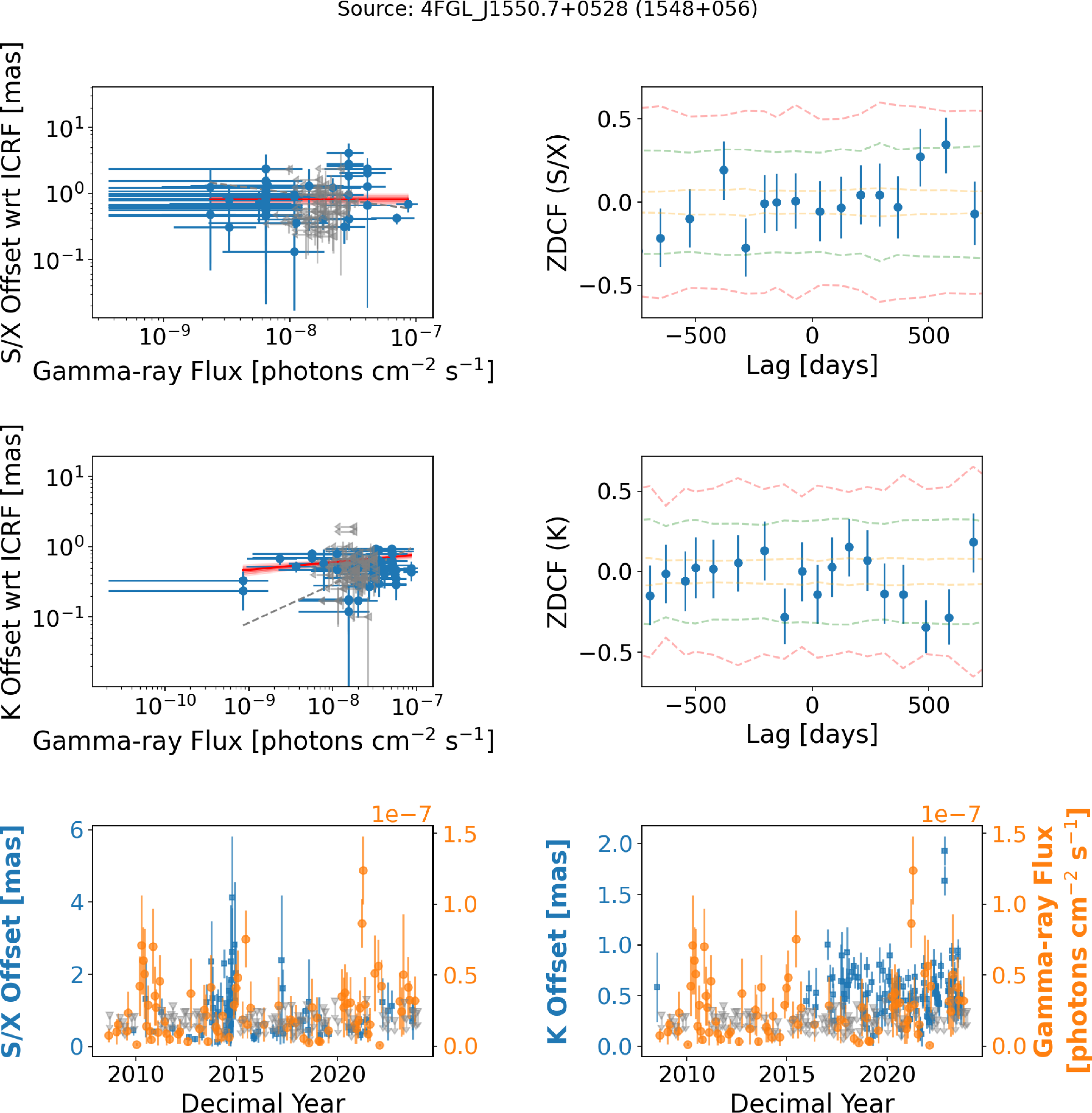
 +
+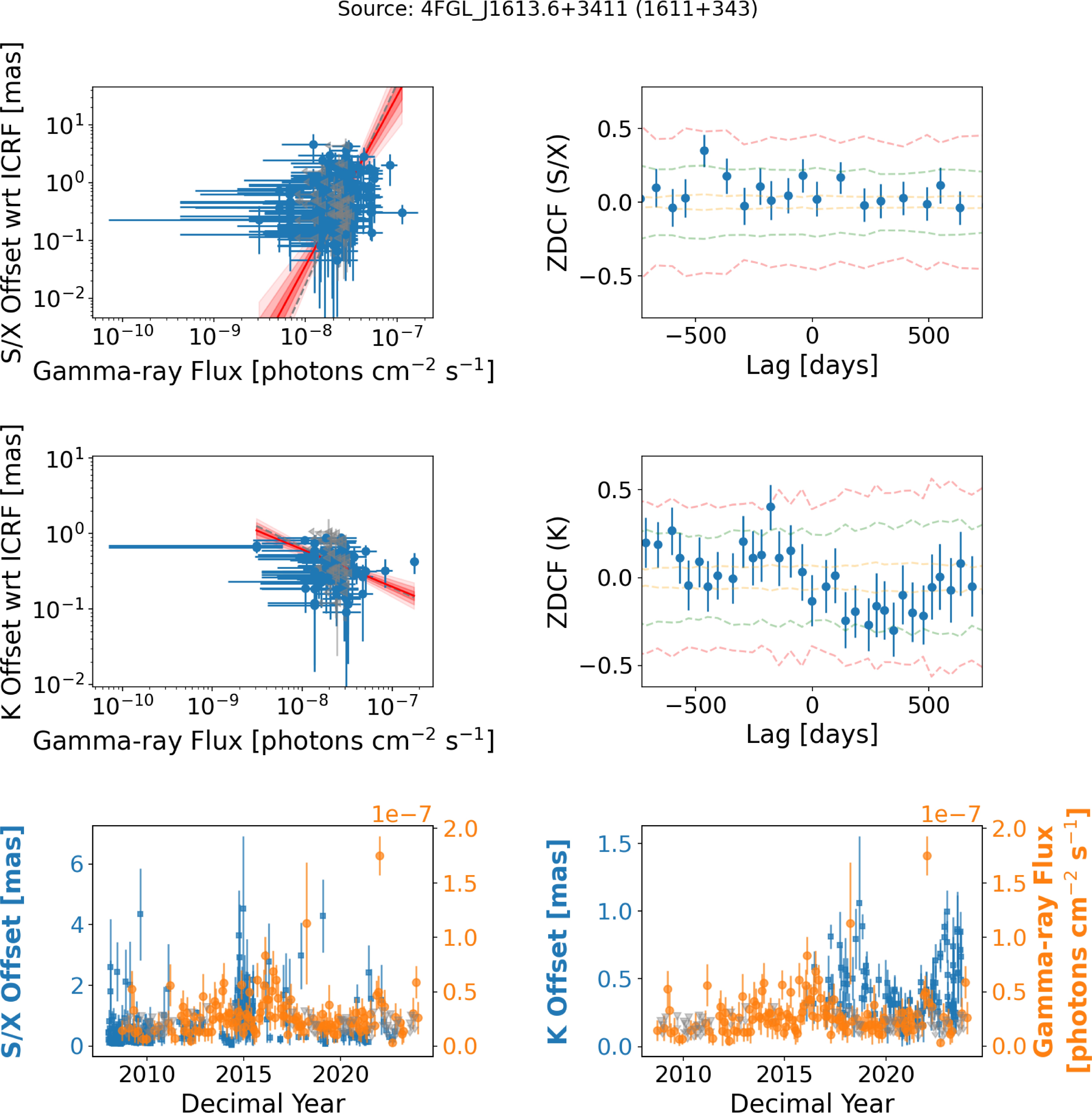
 +
+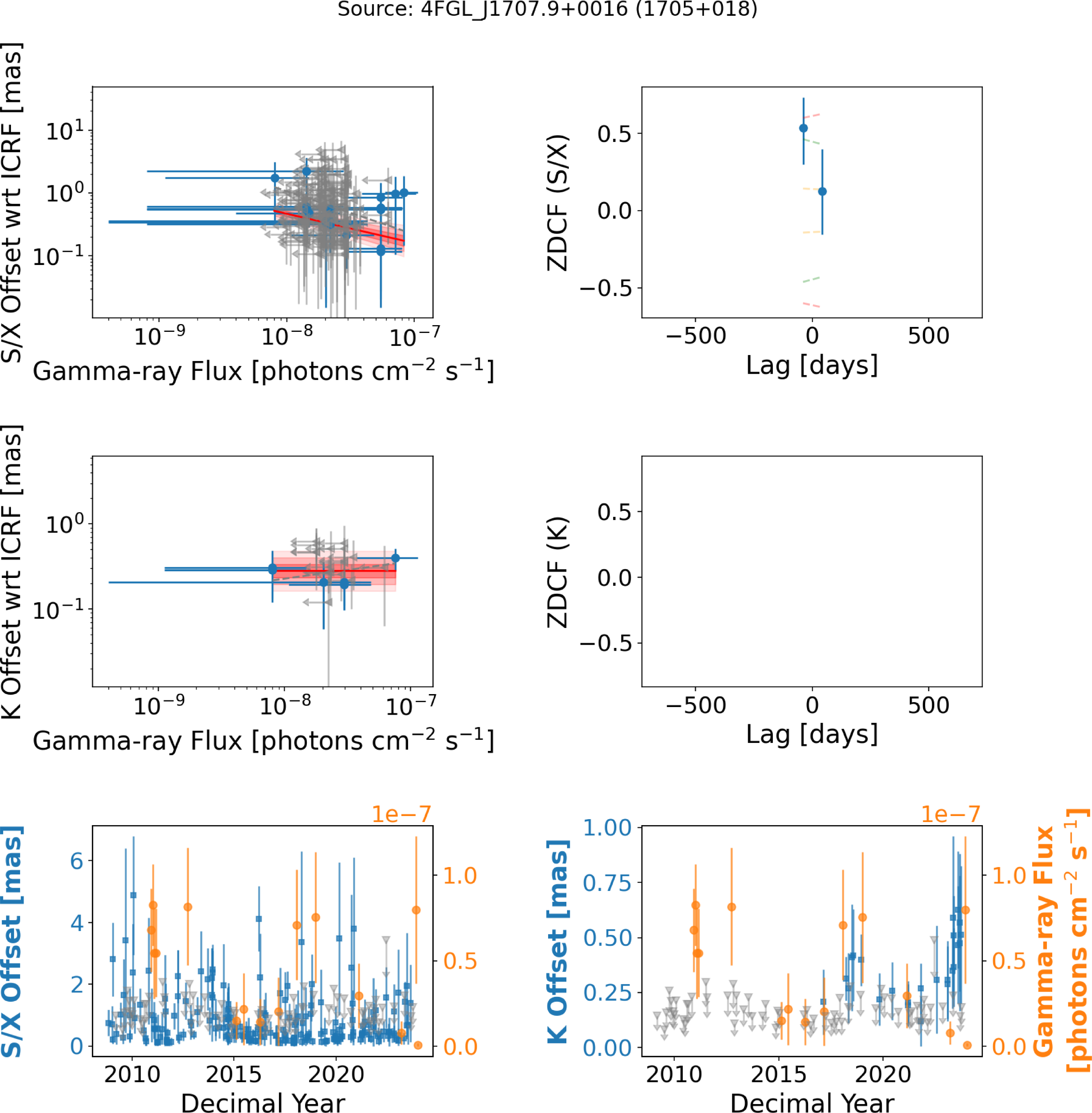
 +
+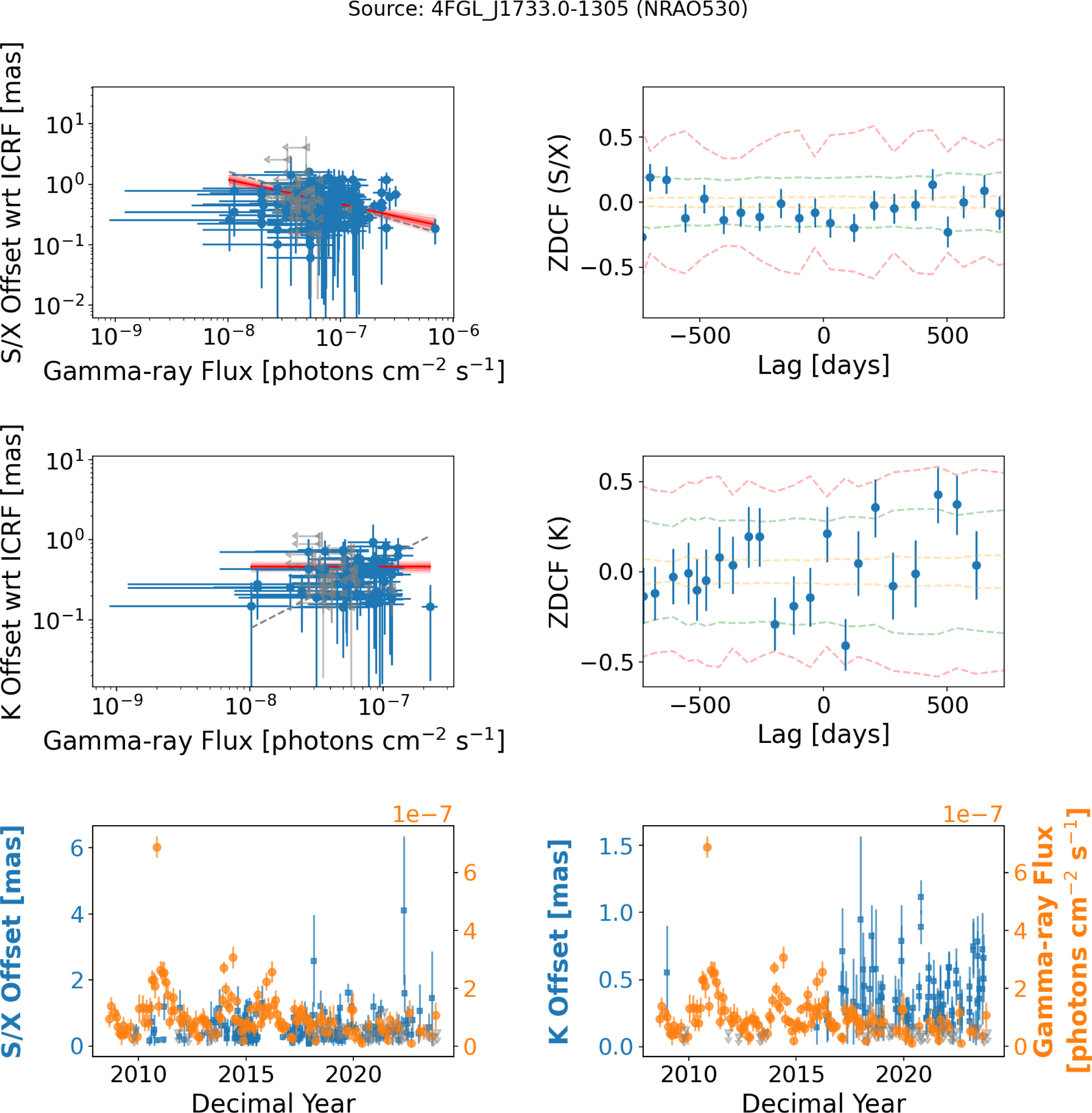
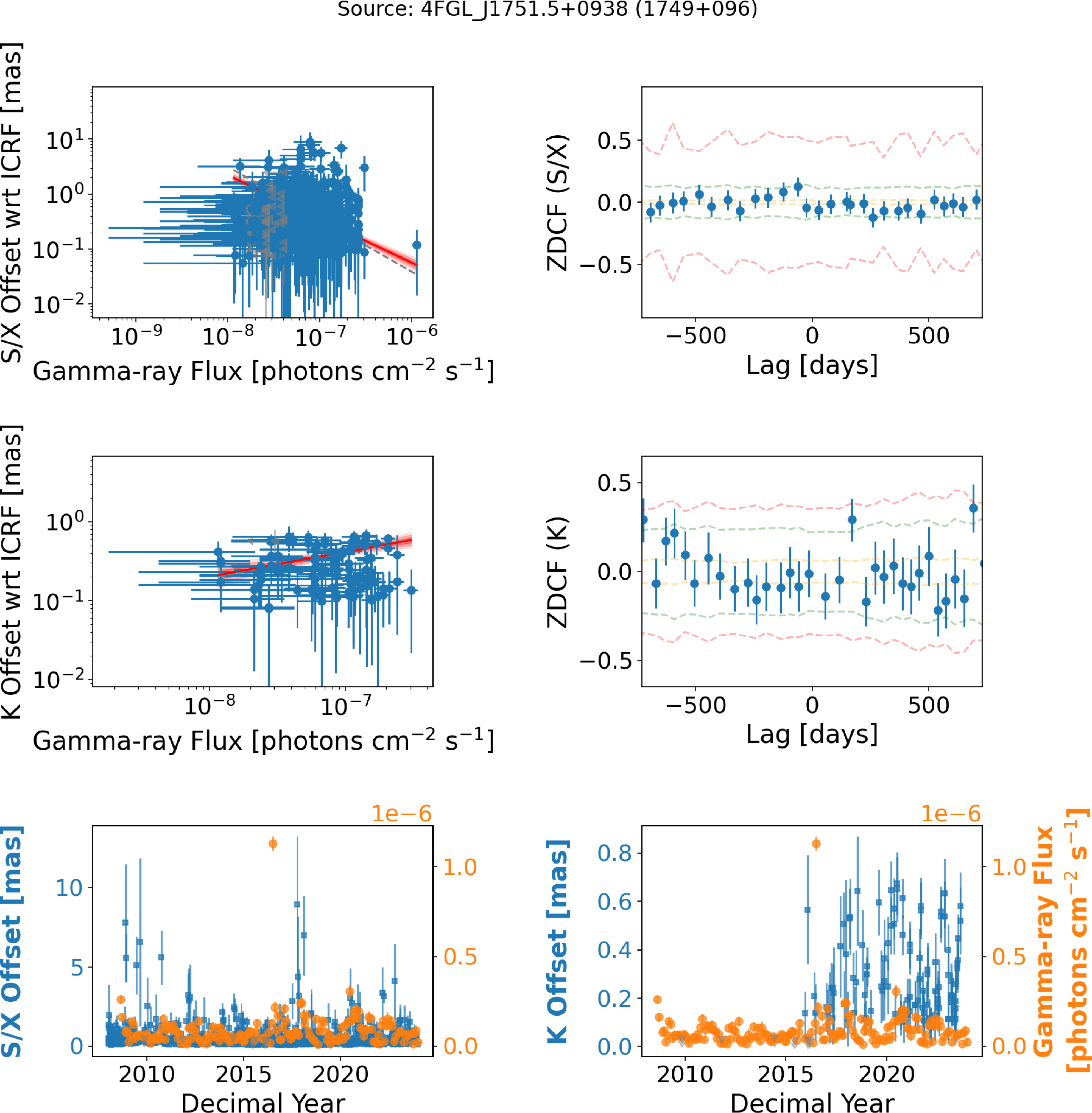
 +
+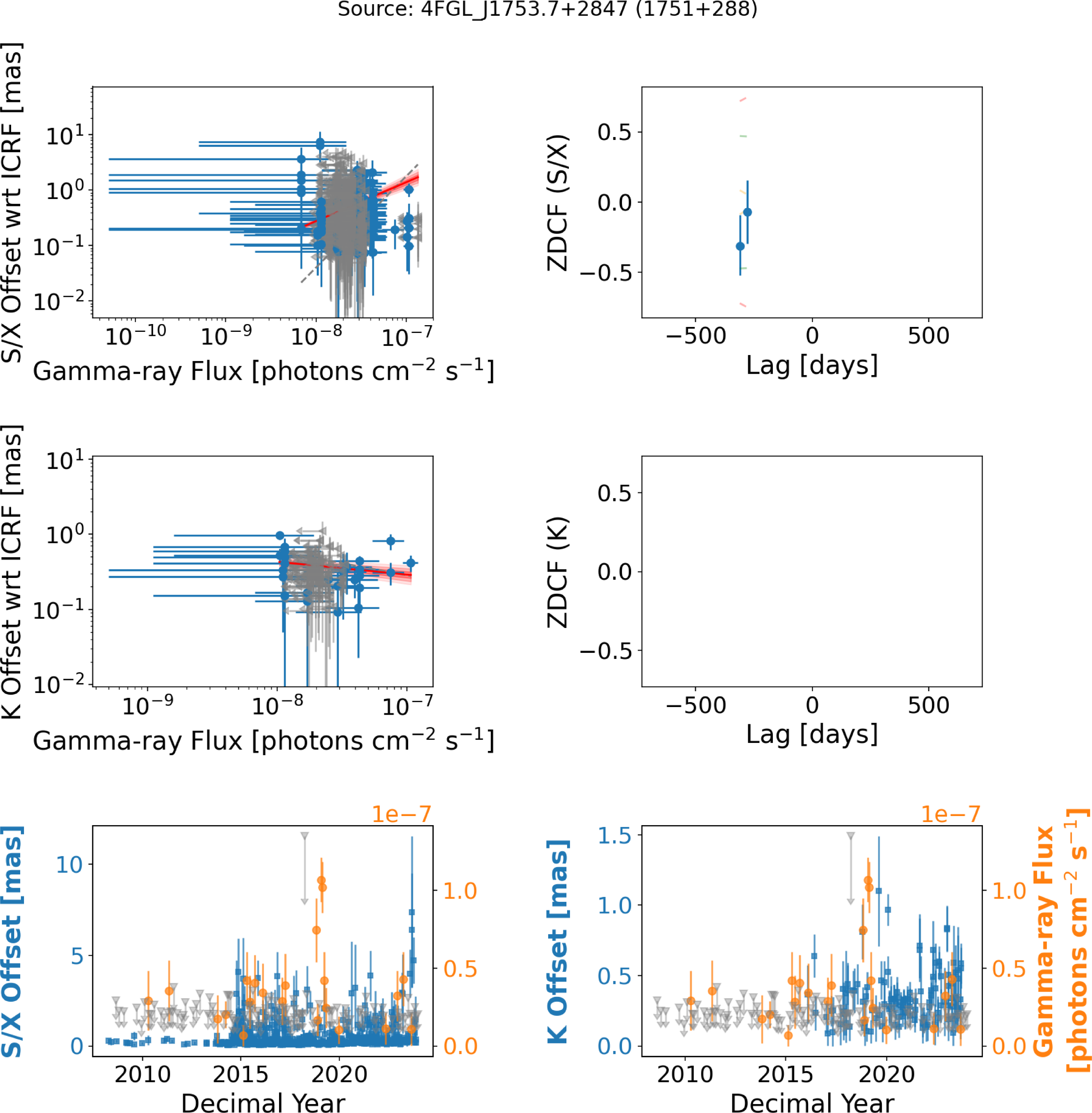
 +
+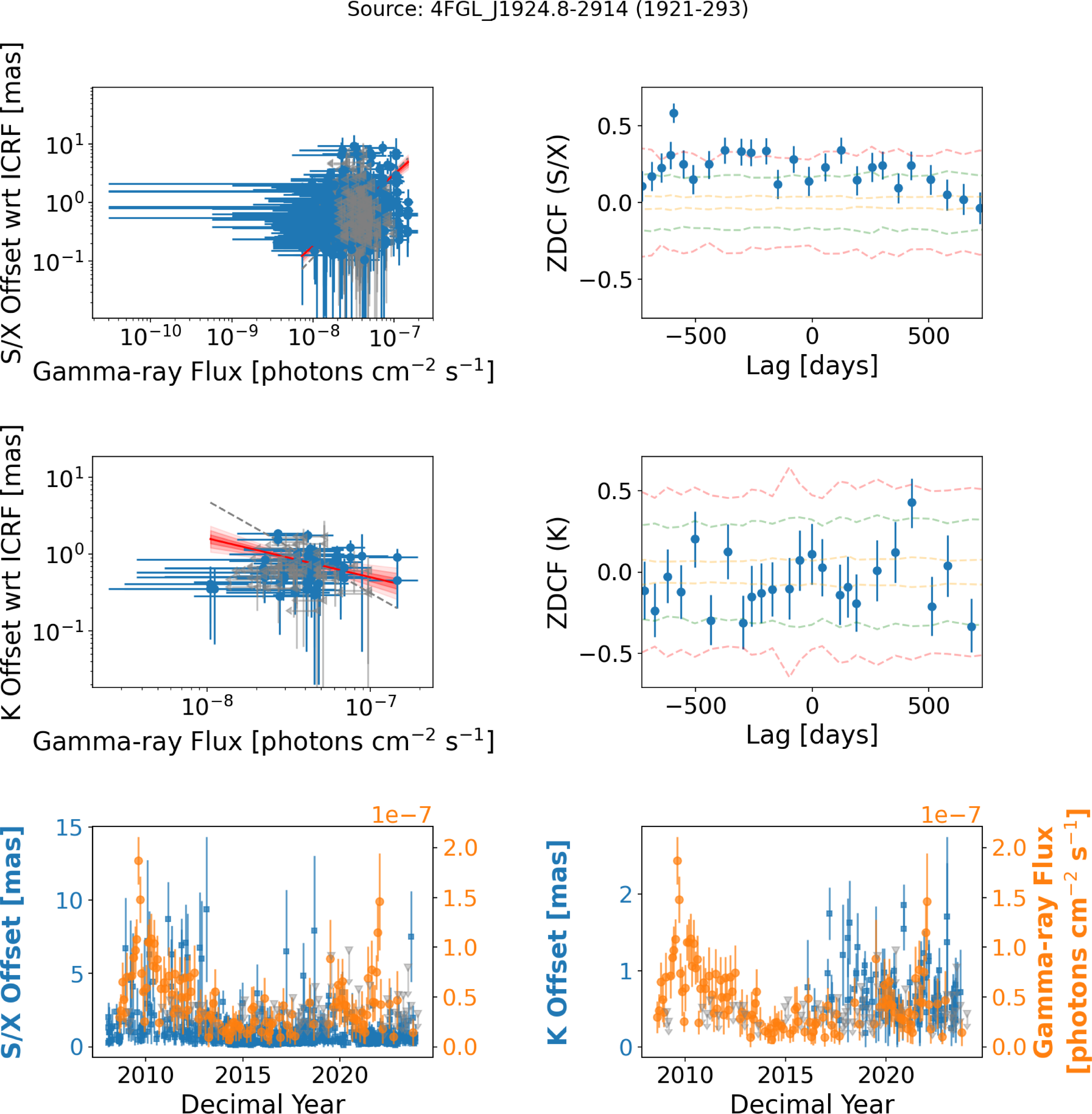
 −
−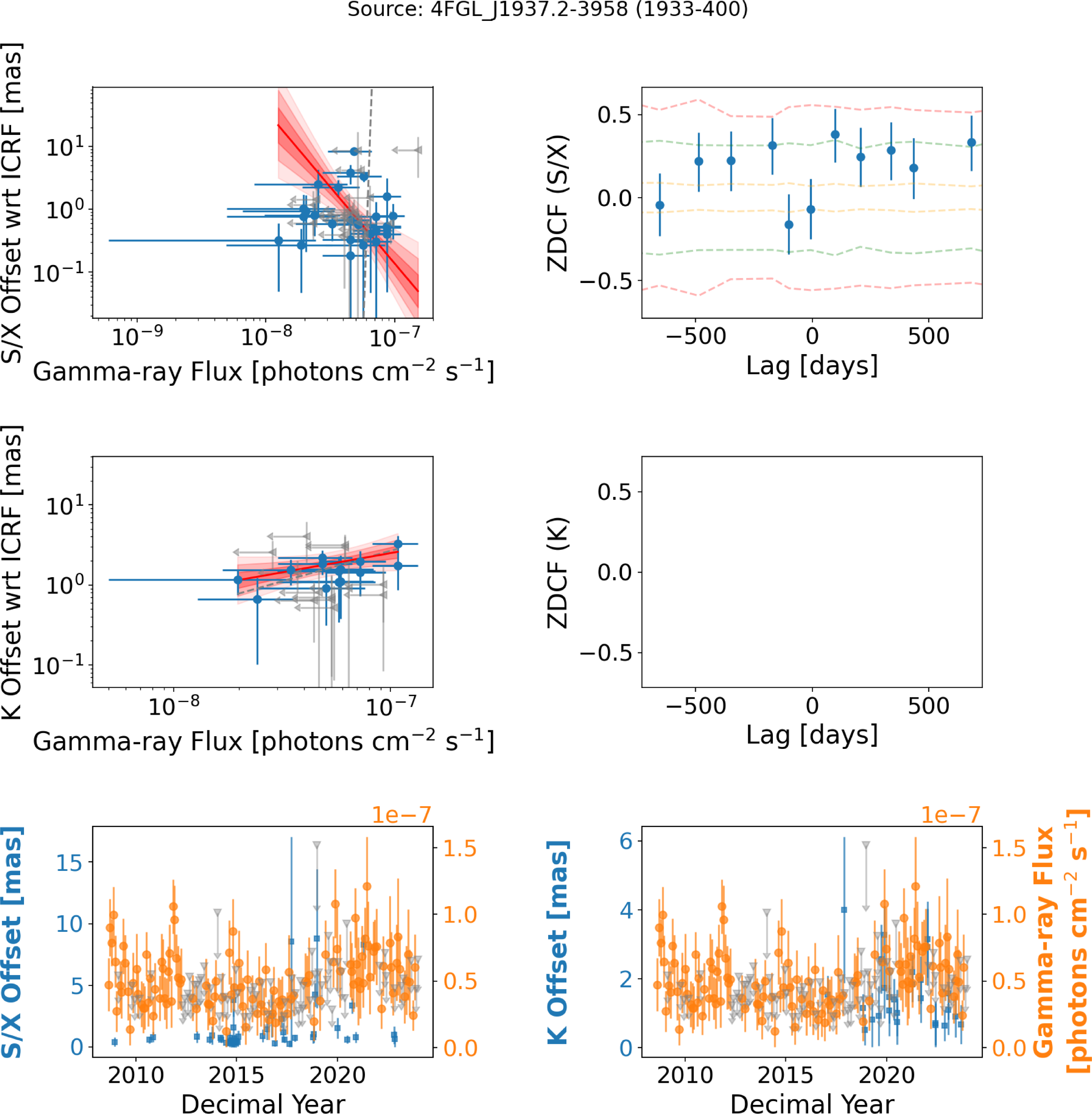
 −
−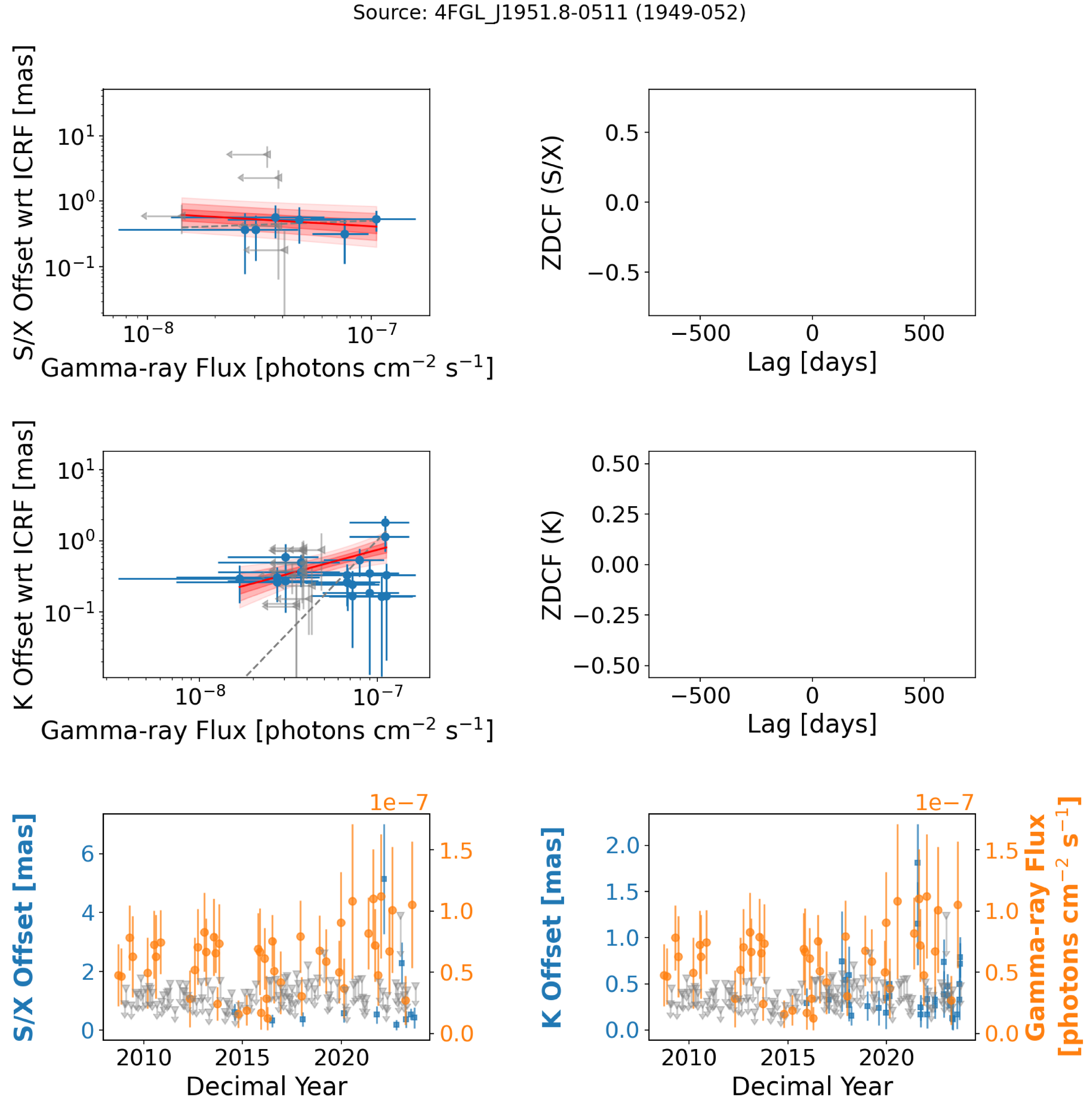
 −
−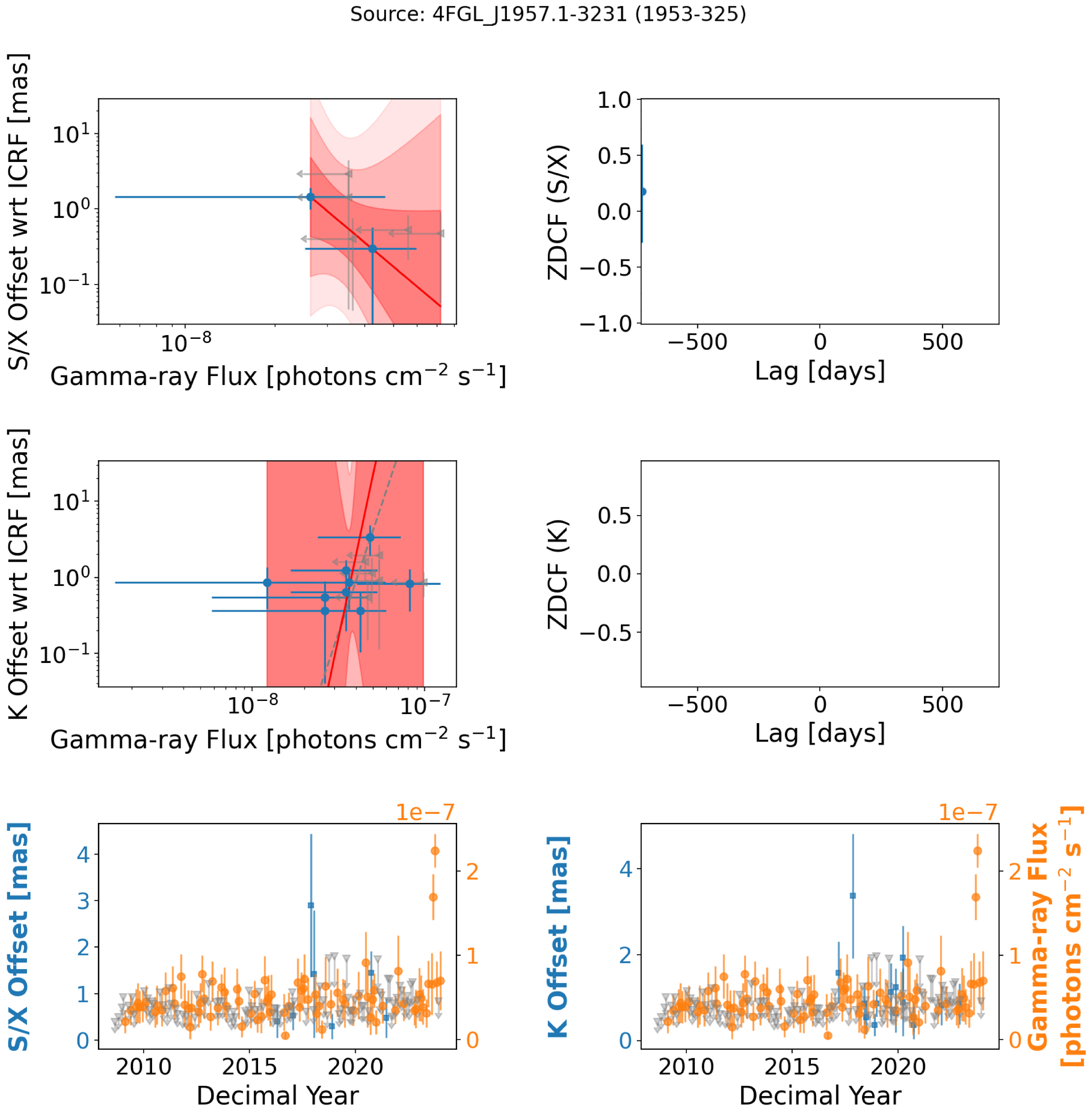
 −
−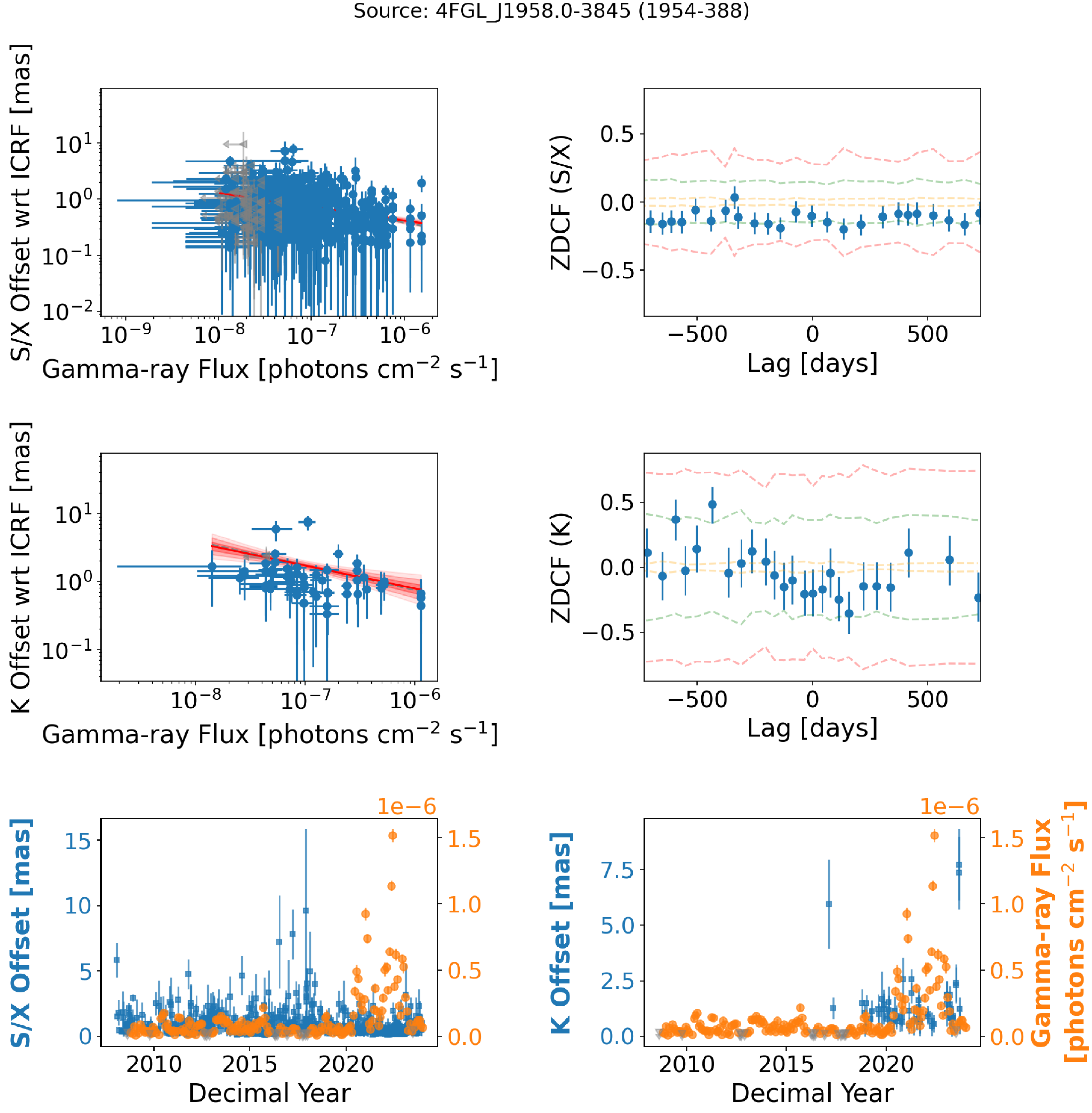
 −
−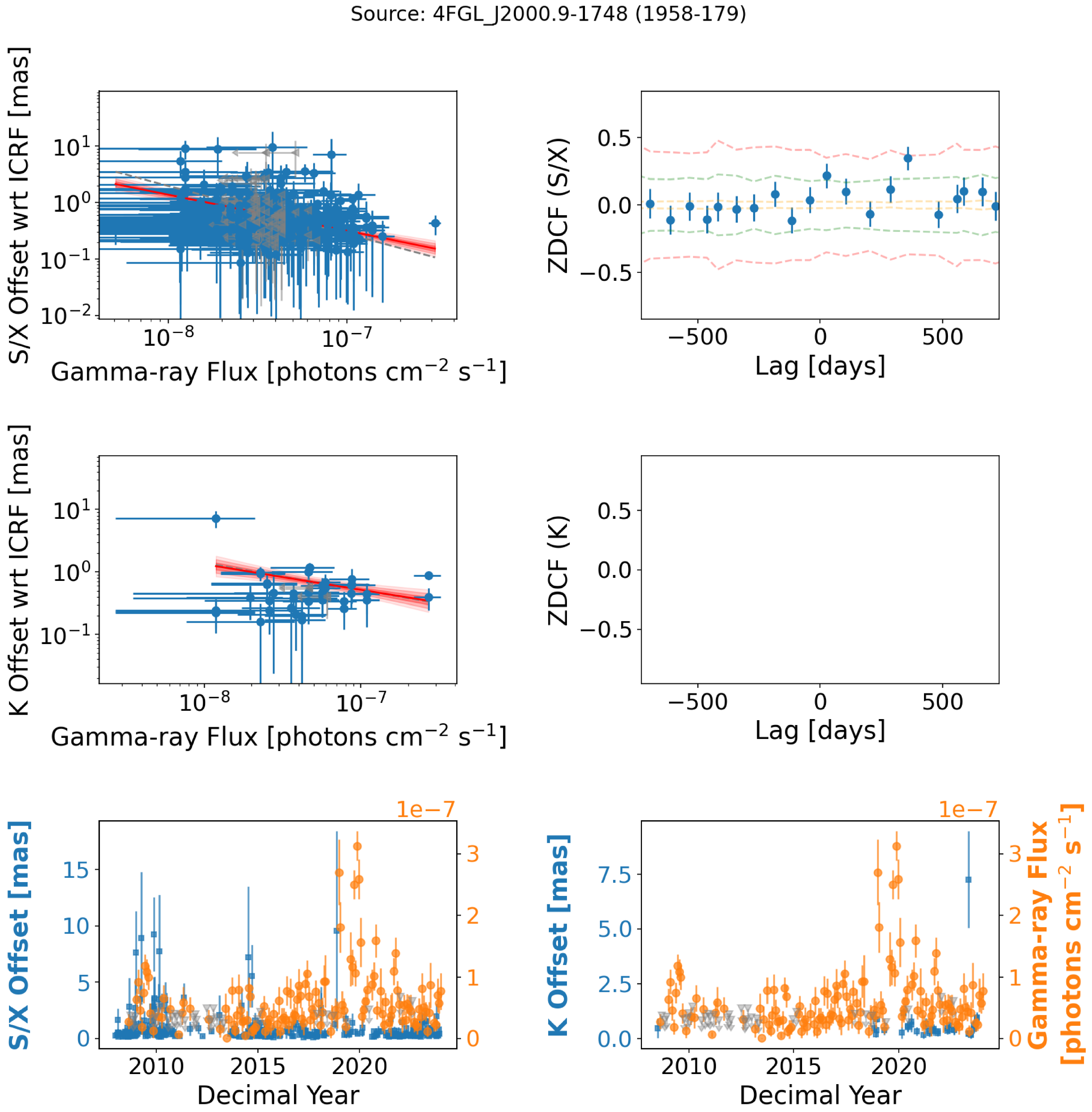
 −
−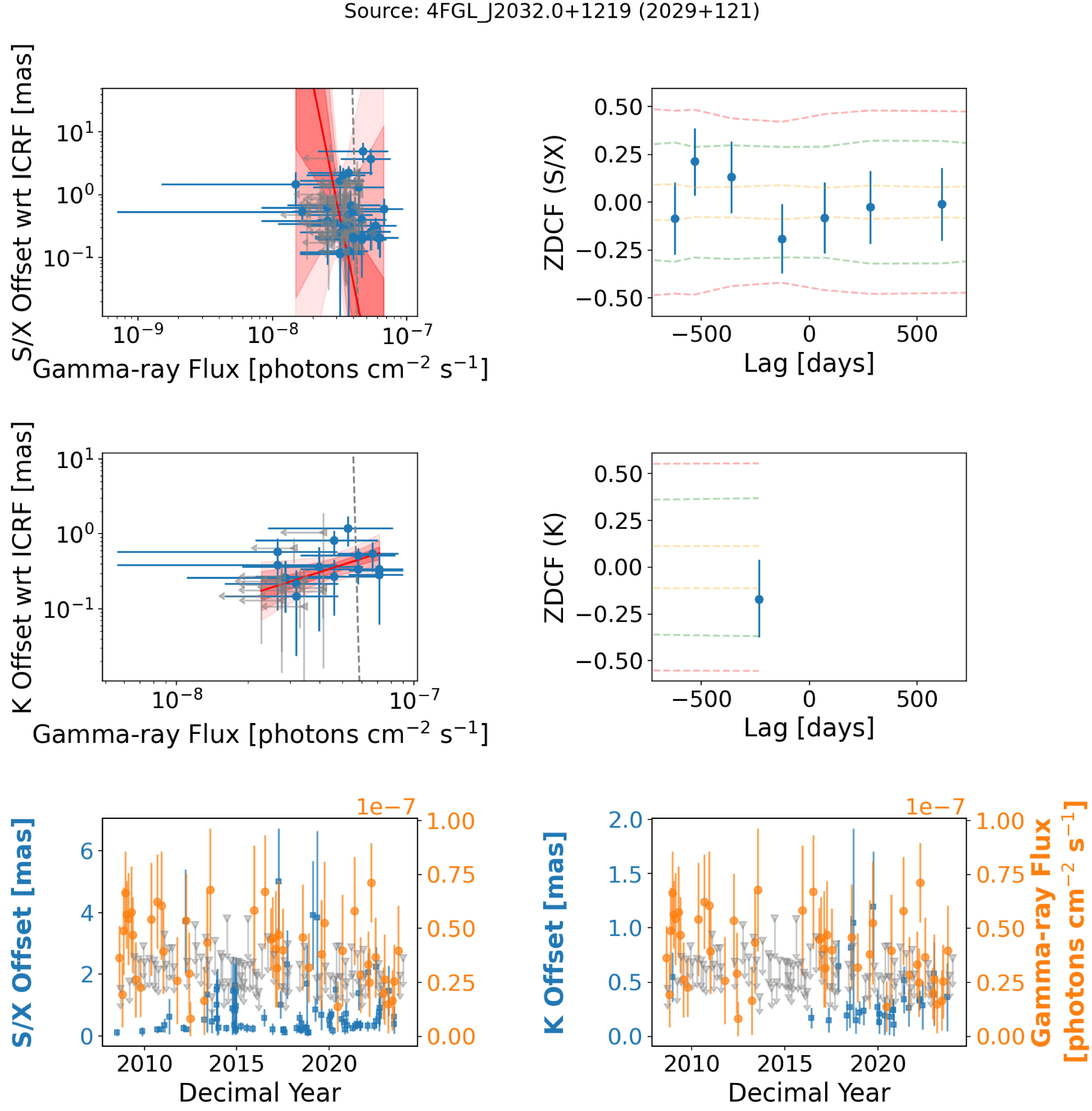
 +
+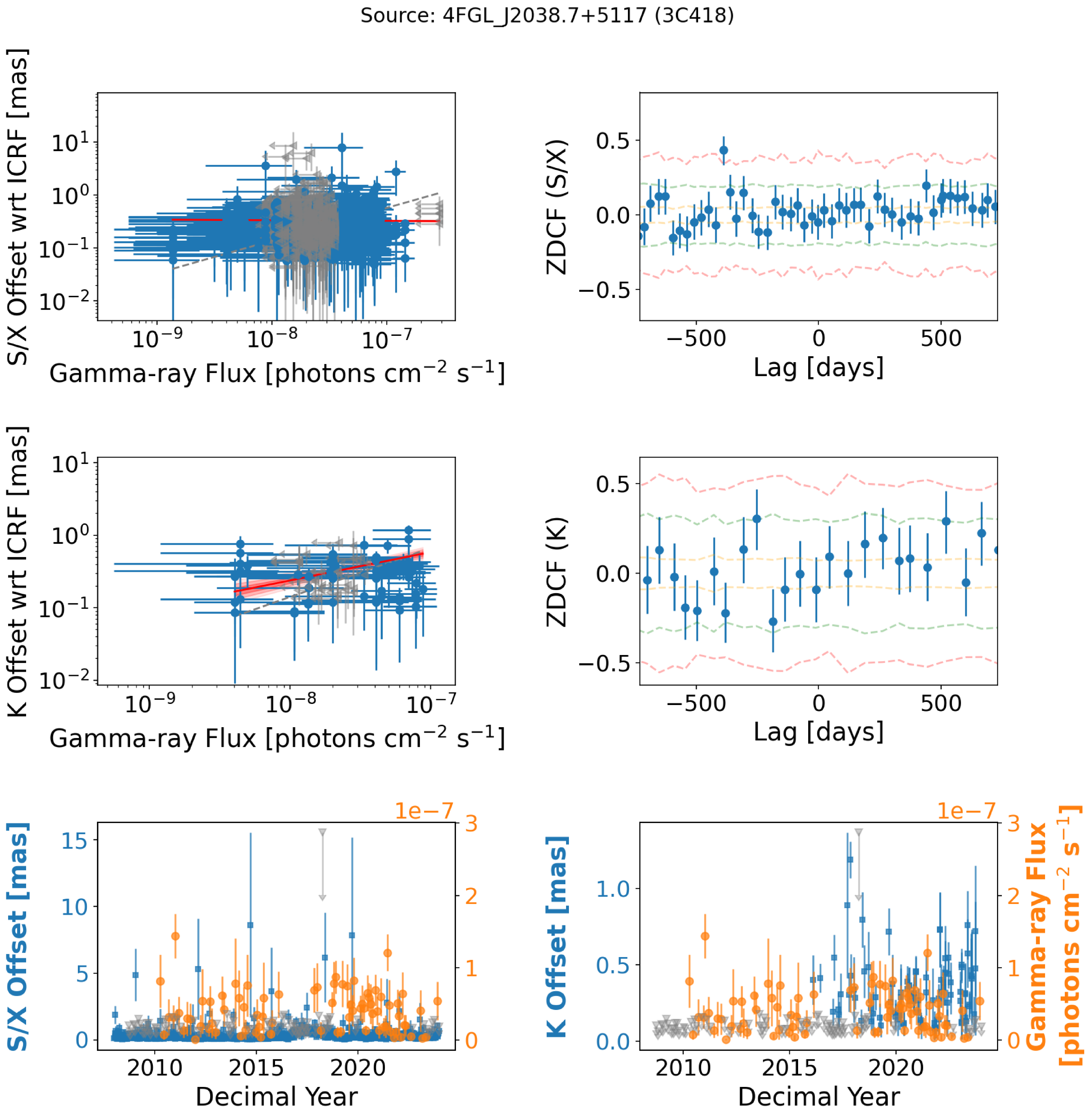
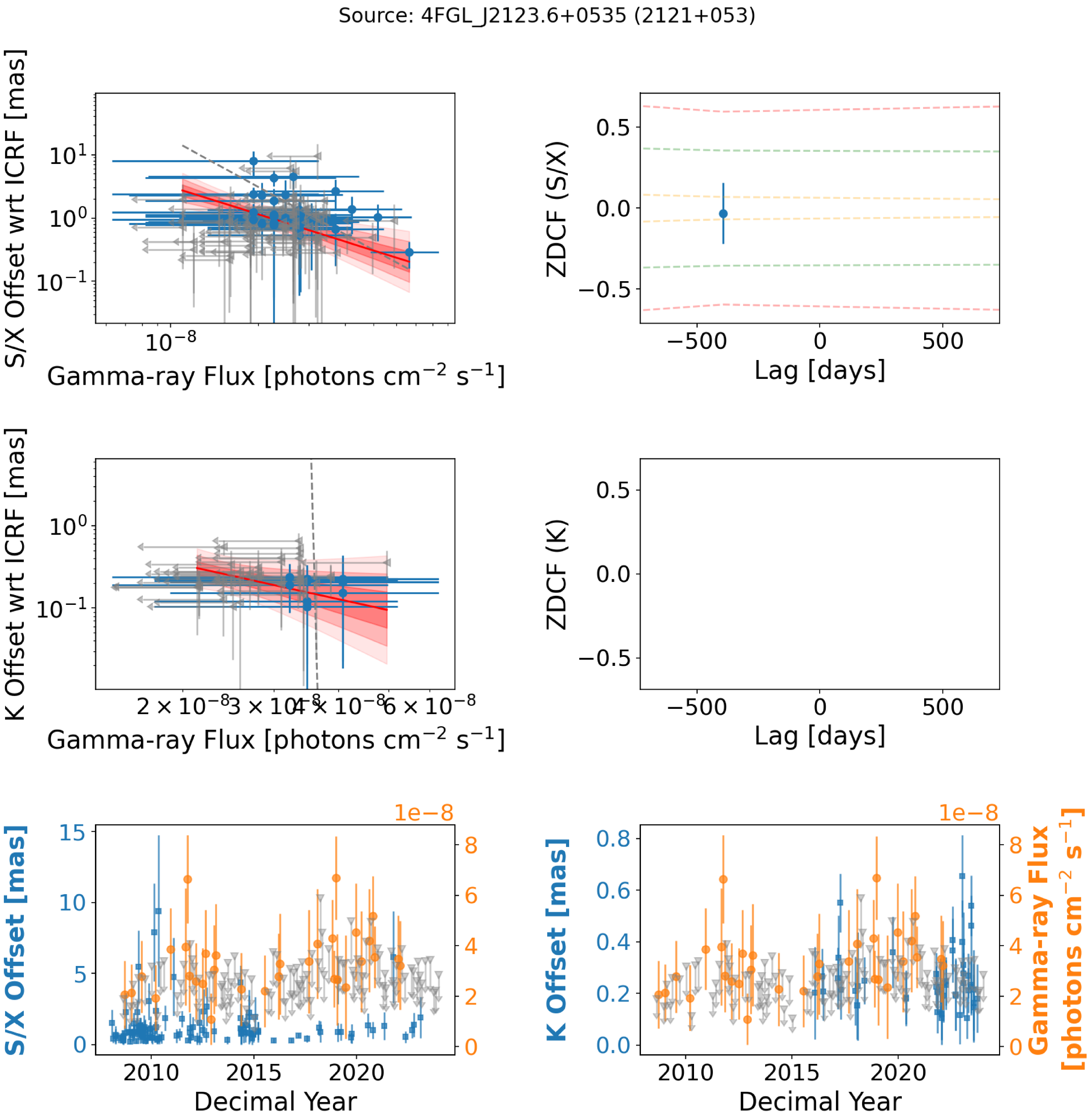
 +
+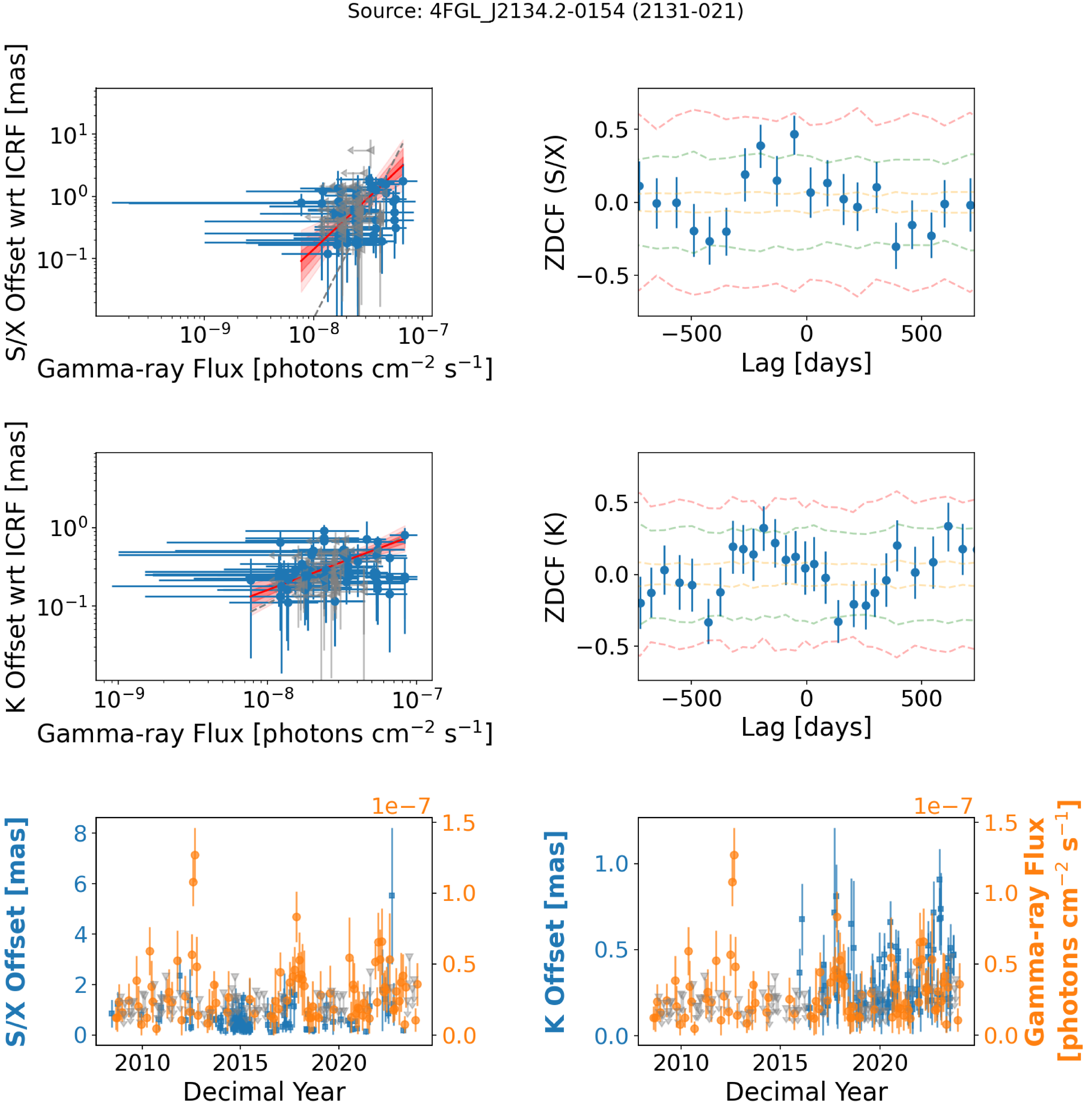
 −
−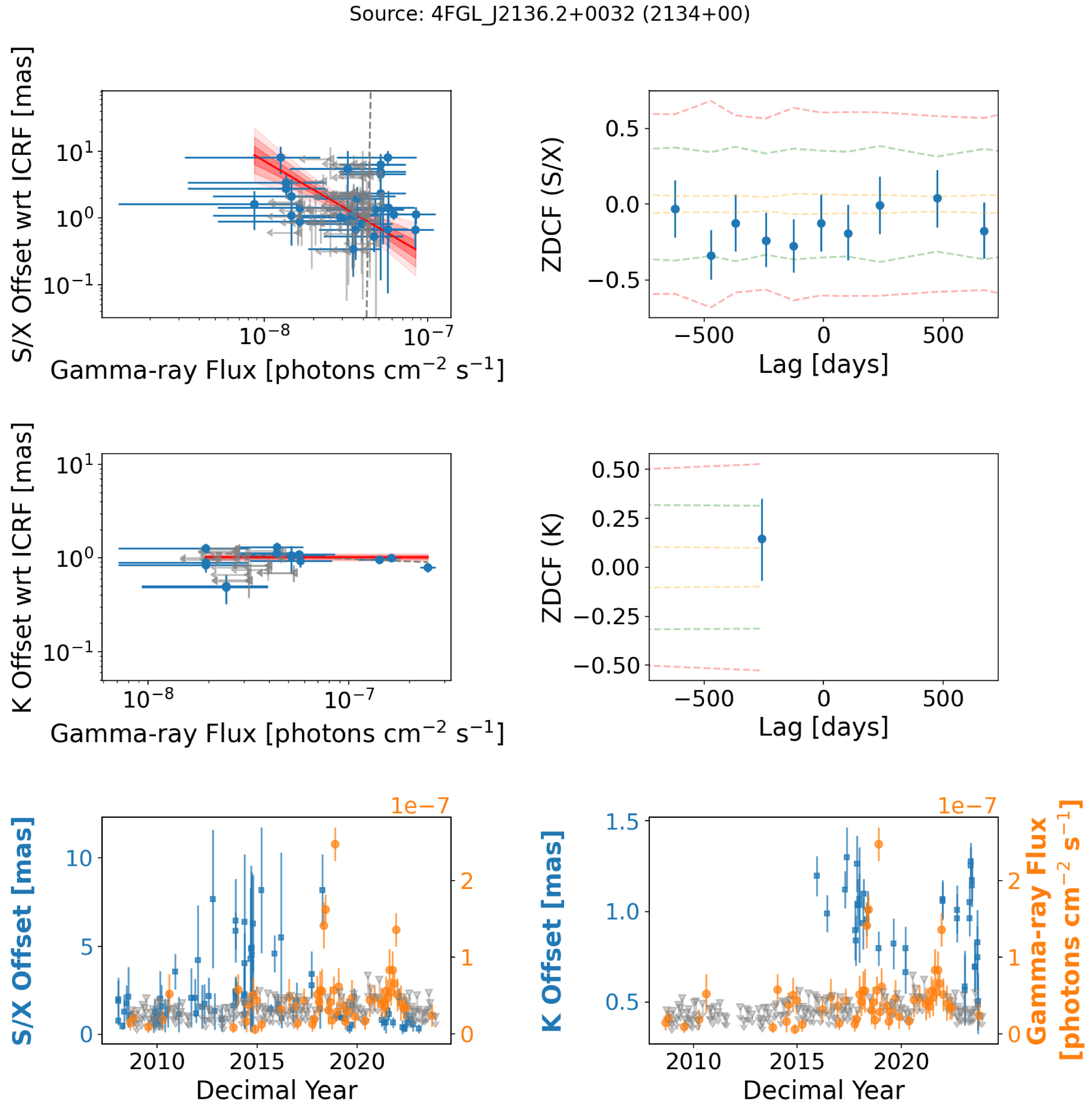
 +
+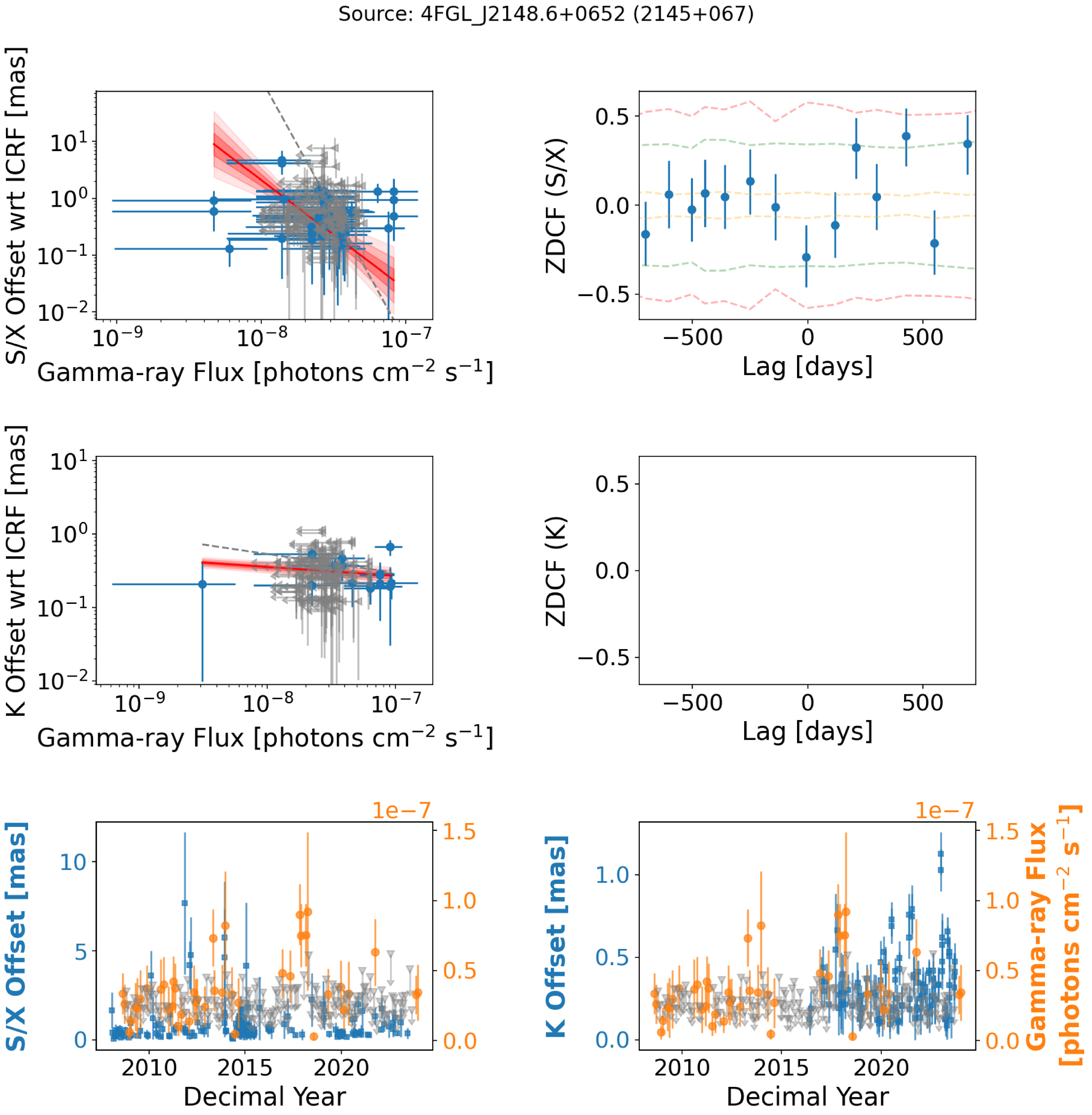
 +
+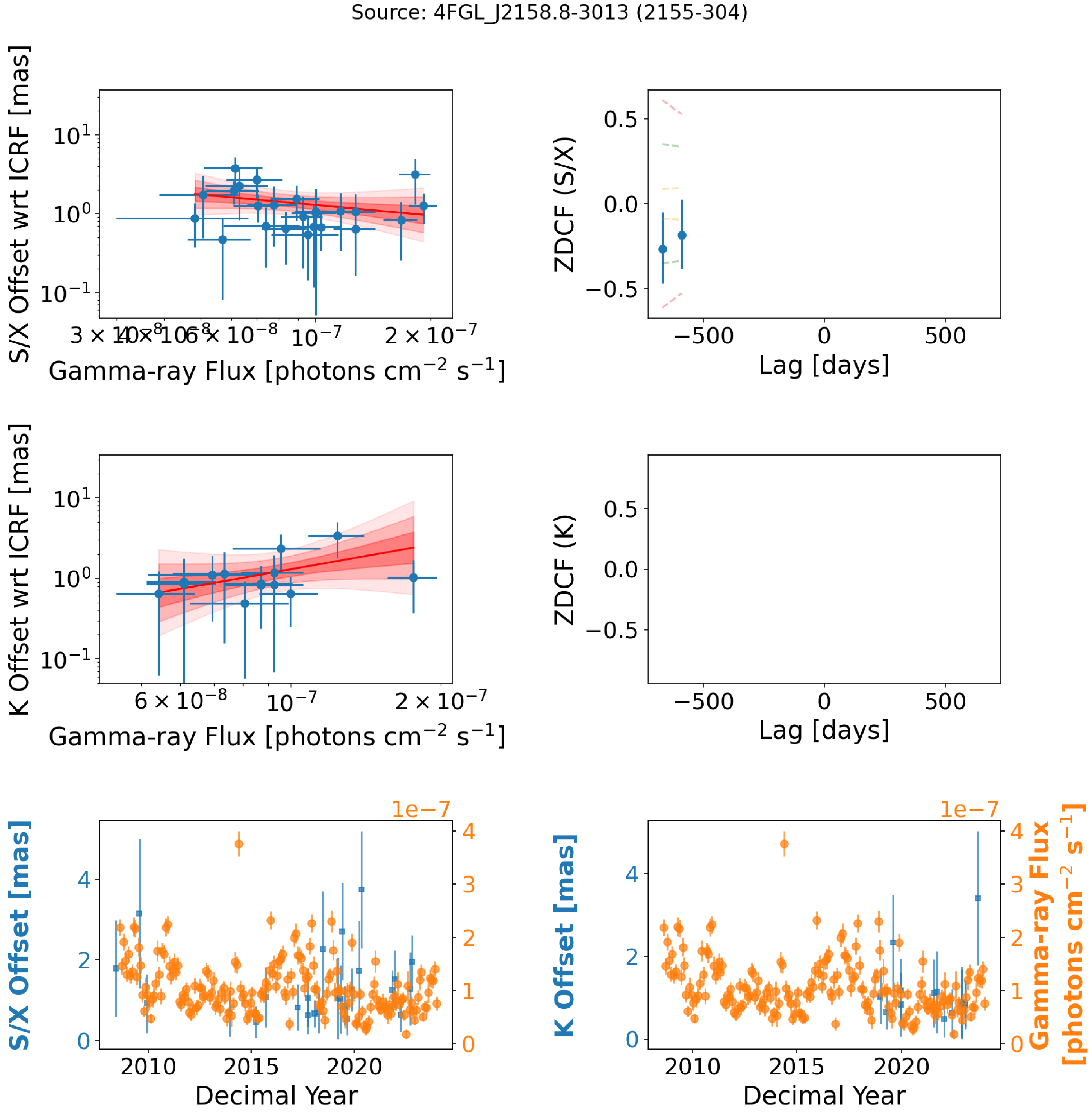
 −
−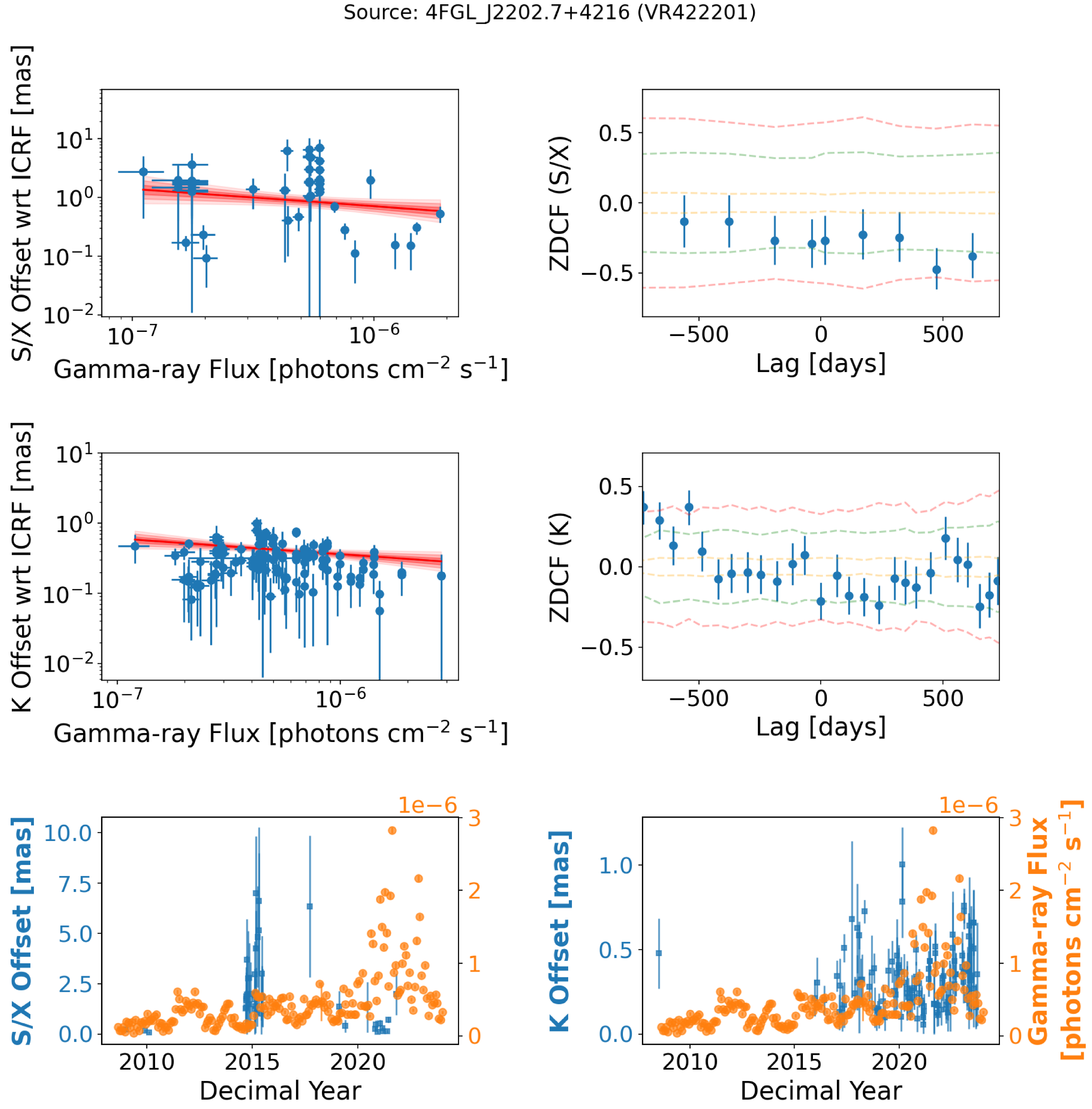
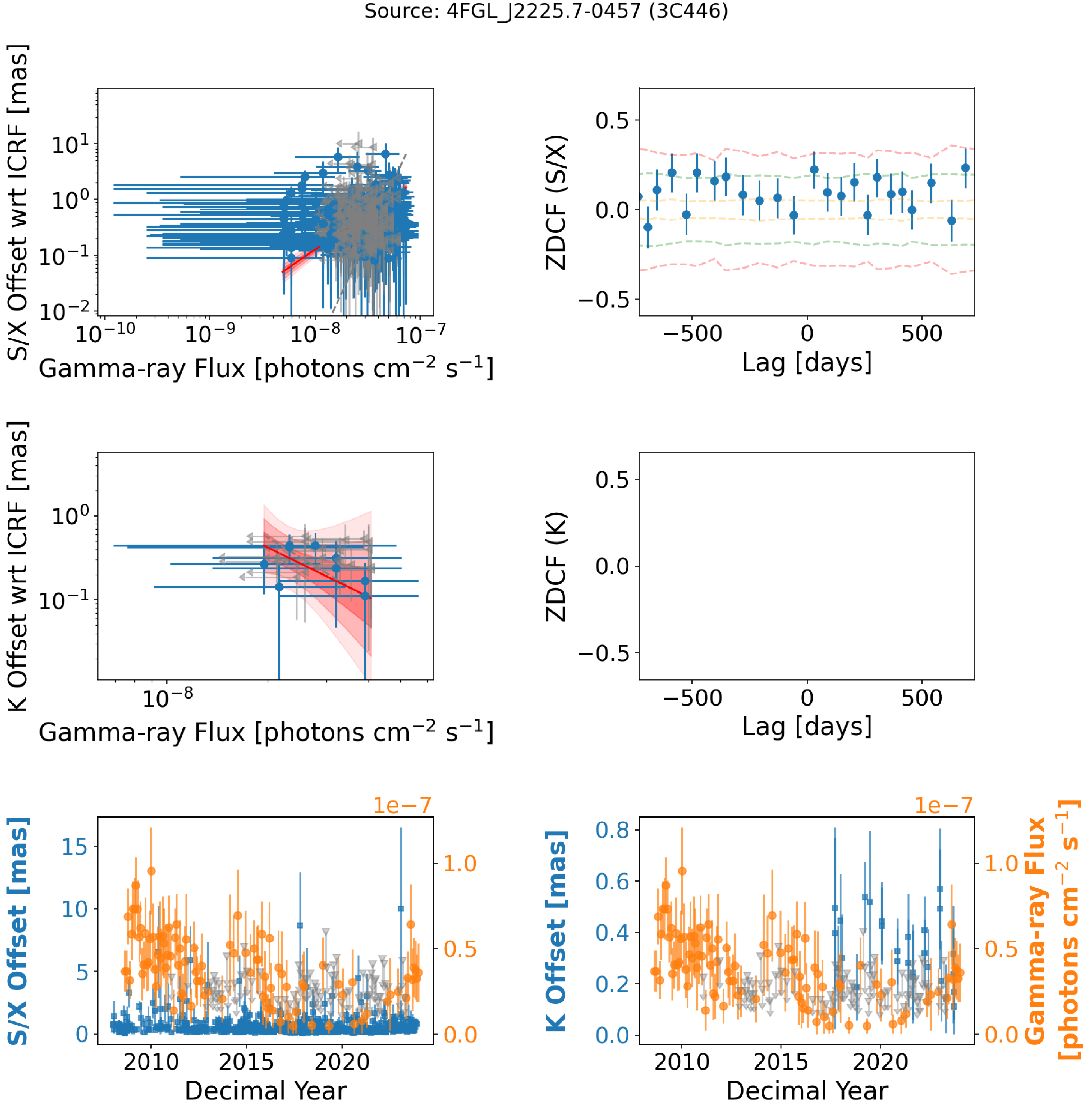
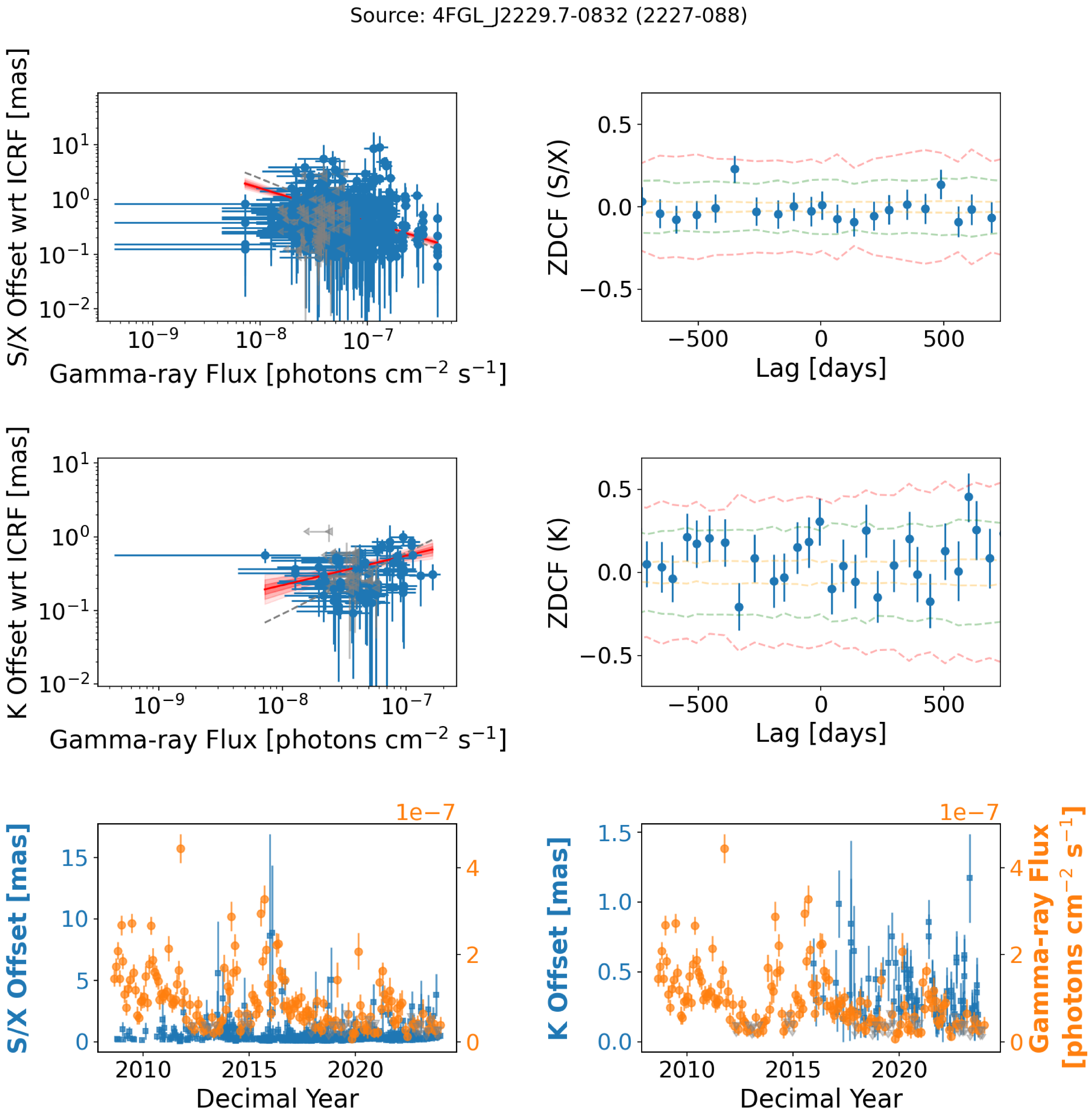
 −
−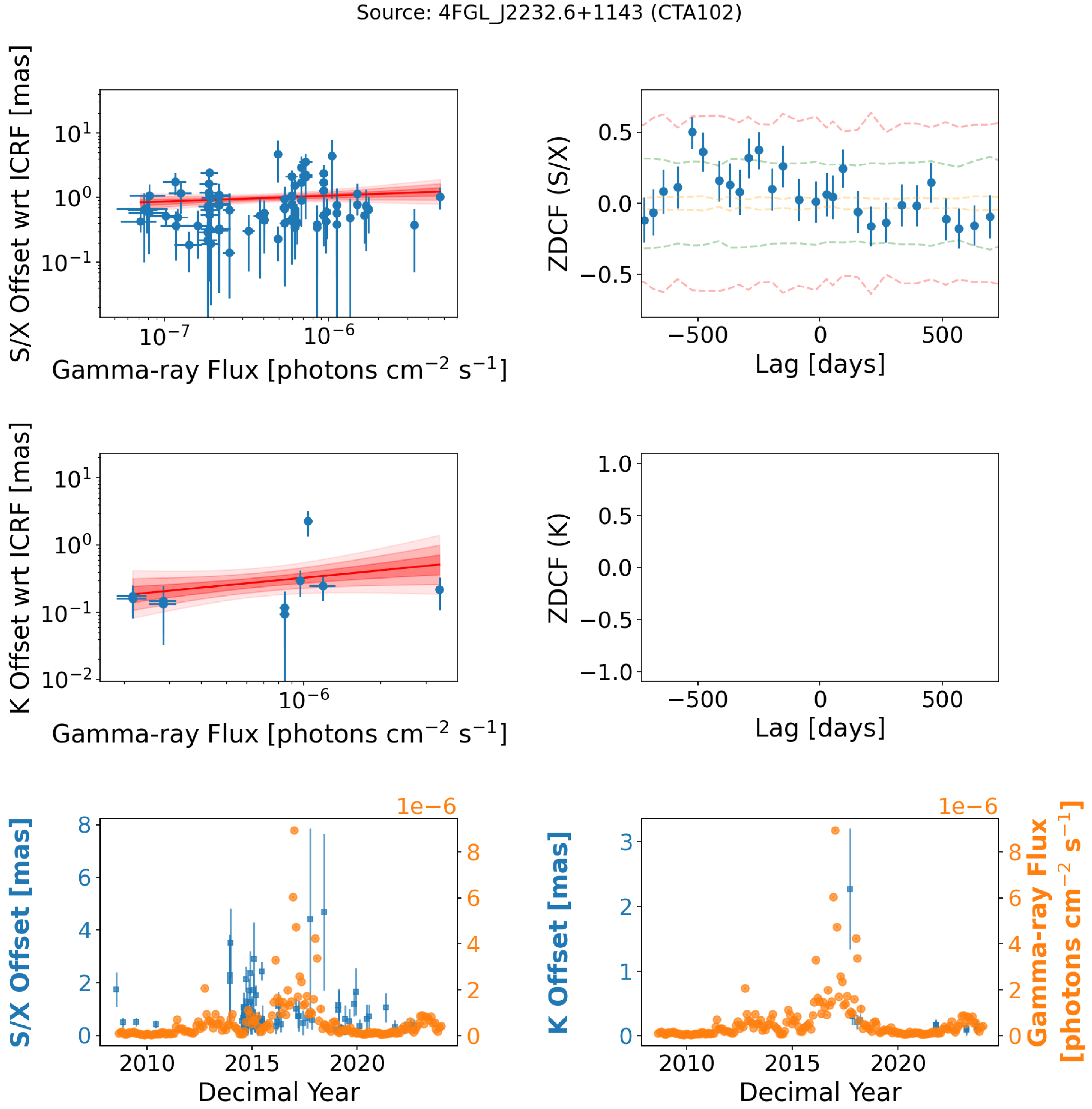
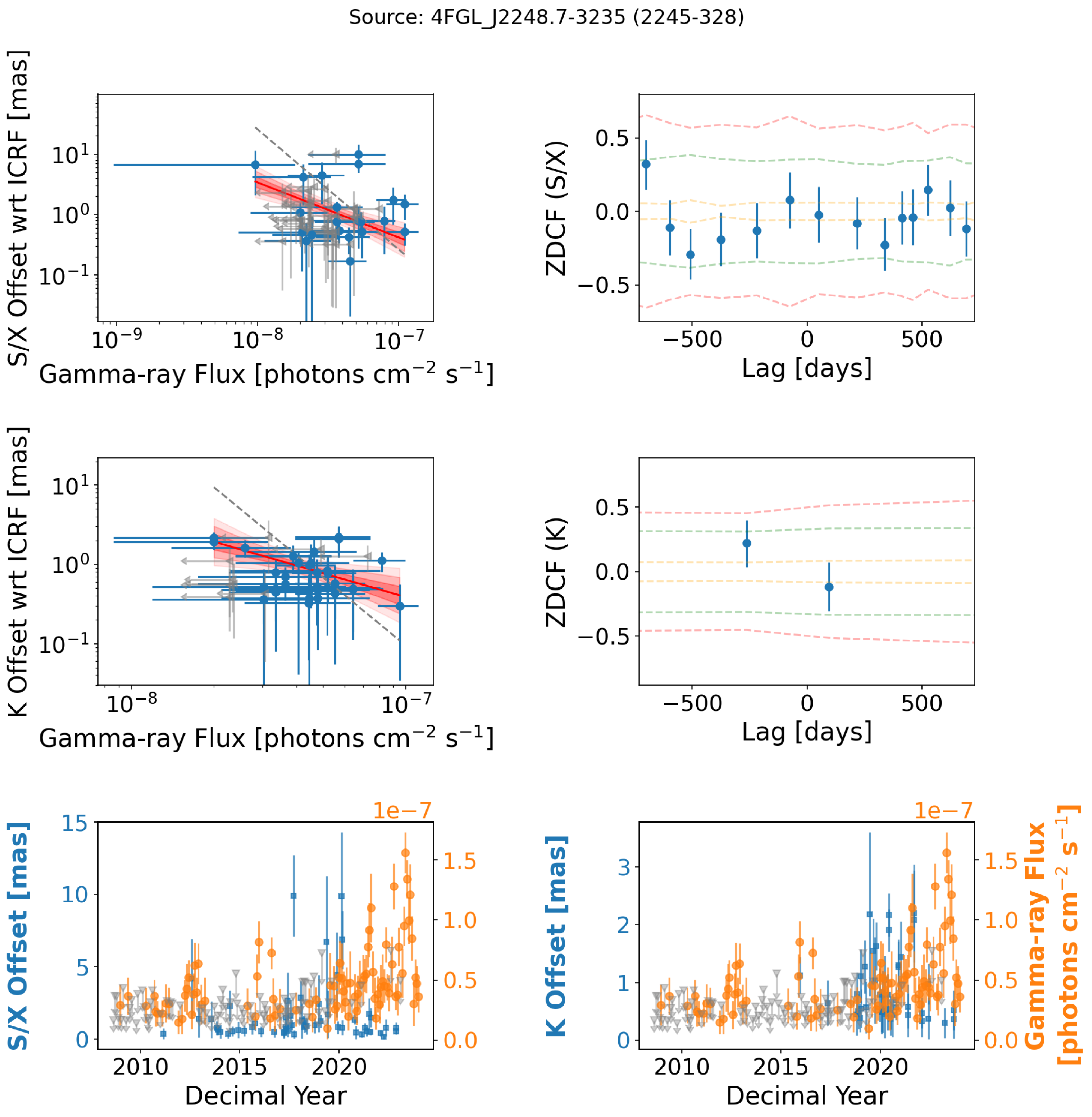
 −
−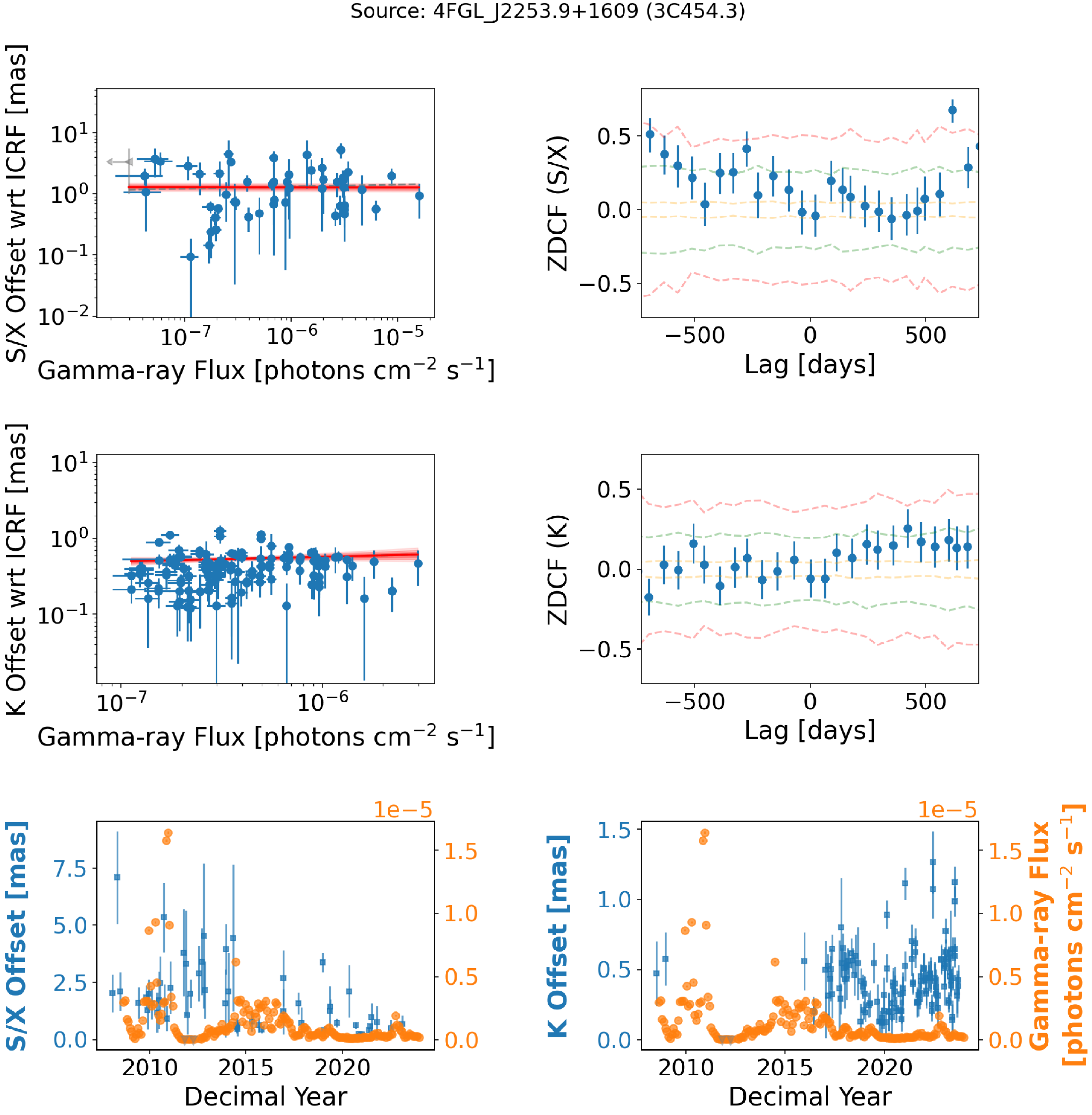
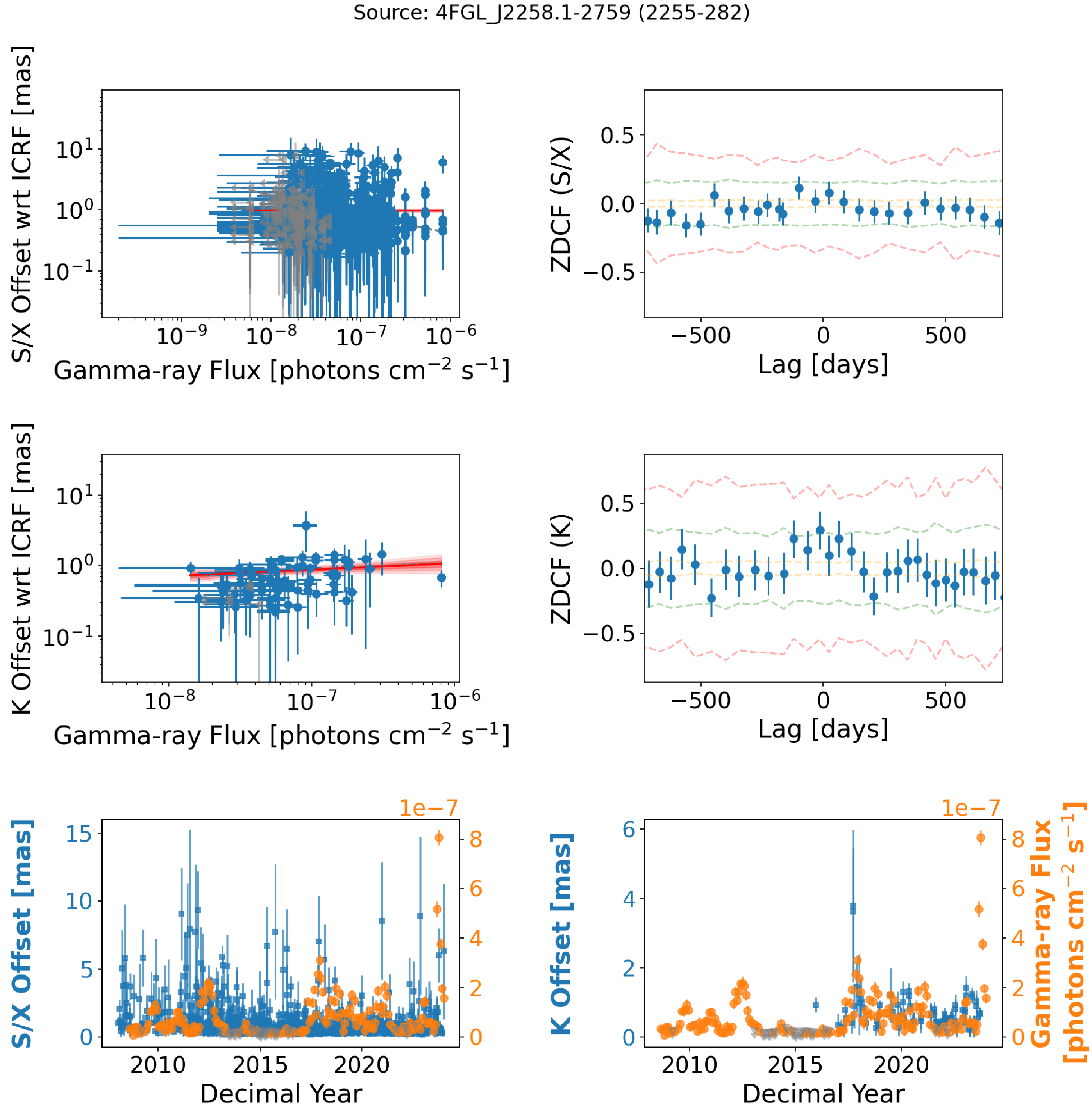
 −
−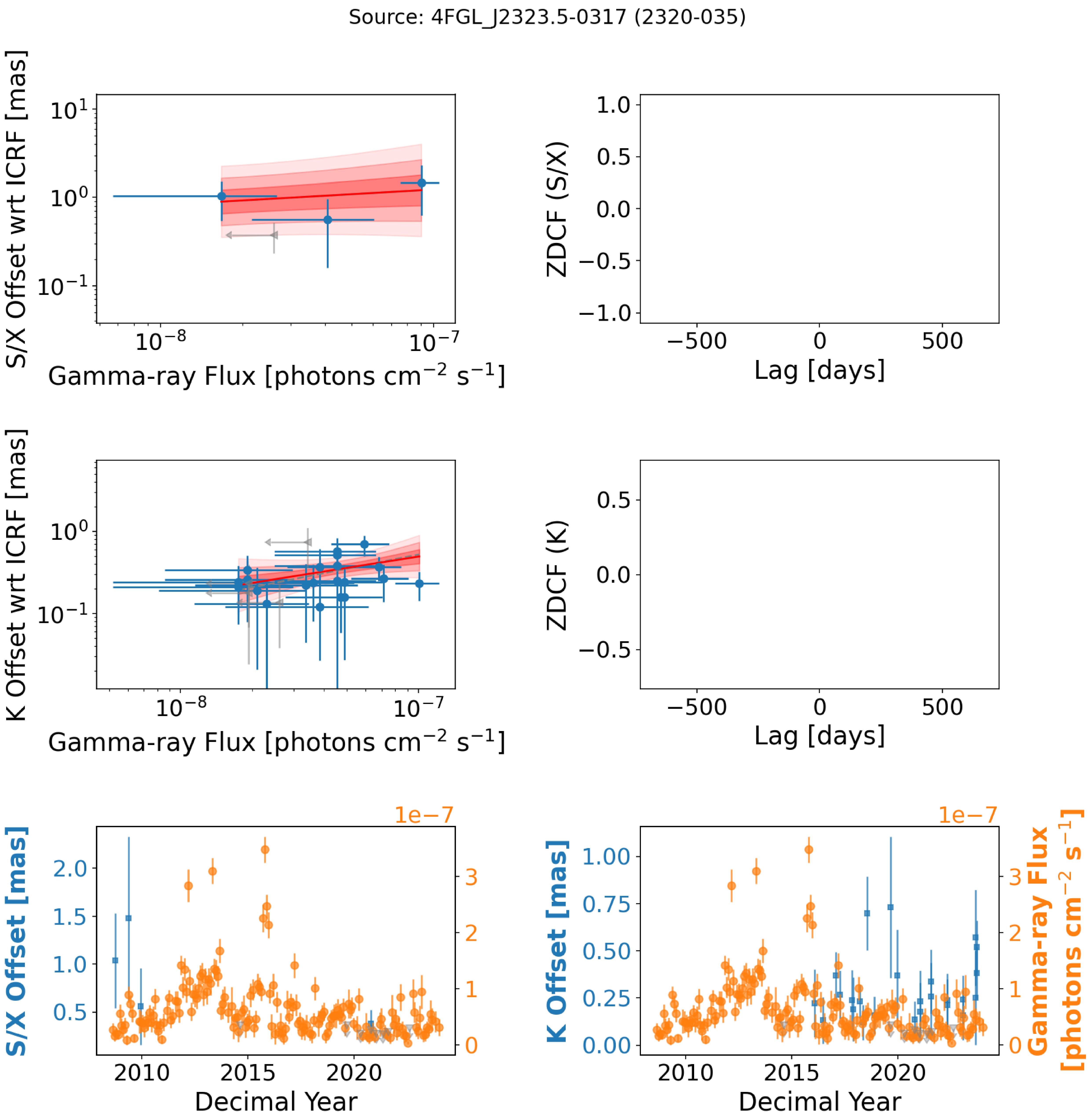
 −
−
 Open access

