


1. Introduction
The distribution of galaxies and their luminosities has previously derived powerful constraints on galaxy evolution (Binggeli, Sandage, & Tammann Reference Binggeli, Sandage and Tammann1988; Benson et al. Reference Benson2003; Rodighiero et al. Reference Rodighiero2010; Gruppioni et al. Reference Gruppioni2013). One of the direct ways of measuring the distribution of galaxies is with the luminosity function (Schechter Reference Schechter1976; Saunders et al. Reference Saunders1990). Luminosity functions (LFs) are statistical distributions that describe the spatial density of astronomical objects and are a fundamental tool for quantifying their evolution across cosmic time scales (Dai et al. Reference Dai2009; Han et al. Reference Han, Dai, Wang, Zhang and Han2012; Wylezalek et al. Reference Wylezalek2014). The use of LFs in galaxy evolution studies has uncovered a wealth of information revealing the intricate processes governing star-formation (SF), galaxy mergers, and the growth of supermassive black holes (SMBH, $M_{BH} \gt 10^{6}\,{\rm M}_{\odot}$
) across cosmic time (Caputi et al. Reference Caputi2007; Hopkins, Richards, & Hernquist Reference Hopkins, Richards and Hernquist2007; Magnelli et al. Reference Magnelli2013; Delvecchio et al. Reference Delvecchio2014; Hernán-Caballero et al. Reference Hernán-Caballero2015). Specifically, many such studies find a strong correlation between the activity of the central SMBH and the star formation rate (SFR) (Hopkins et al. Reference Hopkins, Hernquist, Cox and Kereš2008; Merloni & Heinz Reference Merloni and Heinz2008).
$M_{BH} \gt 10^{6}\,{\rm M}_{\odot}$
) across cosmic time (Caputi et al. Reference Caputi2007; Hopkins, Richards, & Hernquist Reference Hopkins, Richards and Hernquist2007; Magnelli et al. Reference Magnelli2013; Delvecchio et al. Reference Delvecchio2014; Hernán-Caballero et al. Reference Hernán-Caballero2015). Specifically, many such studies find a strong correlation between the activity of the central SMBH and the star formation rate (SFR) (Hopkins et al. Reference Hopkins, Hernquist, Cox and Kereš2008; Merloni & Heinz Reference Merloni and Heinz2008).
Active galactic nuclei (AGN) are actively accreting SMBHs, whereby massive quantities of gas and dust power their growth (Hopkins et al. Reference Hopkins, Hernquist, Cox and Kereš2008; Han et al. Reference Han, Dai, Wang, Zhang and Han2012; Toba et al. Reference Toba2013; Brown et al. Reference Brown2019). It is widely accepted that most galaxies, particularly those with significant bulges, host a SMBH at their centre (Gruppioni et al. Reference Gruppioni, Pozzi, Zamorani and Vignali2011; Han et al. Reference Han, Dai, Wang, Zhang and Han2012; Brown et al. Reference Brown2019). While not all central SMBHs are currently active, such as Sagittarius A $^{*}$
at the centre of our own Milky Way (Event Horizon Telescope Collaboration et al. 2022), most galaxies have likely experienced the influence of an AGN at some point in their history (Gruppioni et al. Reference Gruppioni, Pozzi, Zamorani and Vignali2011). SF in galaxies similarly requires an extensive reservoir of cool gas to operate (Schawinski et al. Reference Schawinski2007; Cicone et al. Reference Cicone2014). The same interstellar material that powers SF can also fuel AGN growth, leading to an inherent link between these two processes (Hopkins et al. Reference Hopkins, Hernquist, Cox and Kereš2008; Brown et al. Reference Brown2019). This connection has fuelled an ongoing debate over whether AGN activity enhances SF by triggering gas inflows or diminishes it through feedback mechanisms that deplete gas reservoirs (Grazian et al. Reference Grazian2015; Fiore et al. Reference Fiore2017).
$^{*}$
at the centre of our own Milky Way (Event Horizon Telescope Collaboration et al. 2022), most galaxies have likely experienced the influence of an AGN at some point in their history (Gruppioni et al. Reference Gruppioni, Pozzi, Zamorani and Vignali2011). SF in galaxies similarly requires an extensive reservoir of cool gas to operate (Schawinski et al. Reference Schawinski2007; Cicone et al. Reference Cicone2014). The same interstellar material that powers SF can also fuel AGN growth, leading to an inherent link between these two processes (Hopkins et al. Reference Hopkins, Hernquist, Cox and Kereš2008; Brown et al. Reference Brown2019). This connection has fuelled an ongoing debate over whether AGN activity enhances SF by triggering gas inflows or diminishes it through feedback mechanisms that deplete gas reservoirs (Grazian et al. Reference Grazian2015; Fiore et al. Reference Fiore2017).
Understanding the role of AGN in galaxy evolution is essential, as these processes regulate the growth of the SMBH and the host galaxy’s development. Studies have shown that the most luminous AGN are often preceded by periods of intense SF (Kauffmann et al. Reference Kauffmann2003; Hopkins et al. Reference Hopkins, Hernquist, Cox and Kereš2008; Hopkins & Quataert Reference Hopkins and Quataert2010) suggesting a co-evolutionary relationship. Some of this activity is seen as AGN-driven outflow winds that can expel the interstellar medium (ISM) from the galaxy (Schawinski et al. Reference Schawinski2007; Cicone et al. Reference Cicone2014; Fiore et al. Reference Fiore2017), thereby starving the galaxy of the cold gas needed for both SF and AGN fueling, ultimately shutting down both processes (Hopkins & Quataert Reference Hopkins and Quataert2010). However, Silk (Reference Silk2013) suggested that AGN-driven winds may, under certain conditions, compress gas and dust, thereby enhancing SF. This scenario aligns with findings from Cowley et al. (Reference Cowley2016), which indicate that AGN-dominated systems tend to have higher specific SFRs, suggesting that SF and AGN activity can co-exist in certain environments.
Both SF and AGN activity releases an enormous amount of energy across the entire electromagnetic spectrum, from radio waves to gamma rays (Ho Reference Ho1999; Huang et al. Reference Huang2007; Silva et al. Reference Silva2011; Gruppioni et al. Reference Gruppioni, Pozzi, Zamorani and Vignali2011). LFs at various wavelengths have been used to place powerful constraints on evolutionary models, as seen in Aird et al. (Reference Aird2015), Alqasim & Page (Reference Alqasim and Page2023) (X-ray), Yuan et al. (Reference Yuan, Wang, Worrall, Zhang and Mao2018) (Radio), Page et al. (Reference Page2021) (UV), and Cool et al. (Reference Cool2012) (optical). However, the properties of infrared (IR) light make it the ideal regime for studying SF and AGN LFs as both processes are often dusty and obscured (optically thick) (Wu et al.Reference Wu2011; Han et al. Reference Han, Dai, Wang, Zhang and Han2012).Dust extinction absorbs the outgoing X-ray, optical, and UV wavelengths and re-emits the radiation in the IR domain (Fu et al. Reference Fu2010; Toba et al. Reference Toba2013; O’Connor et al. Reference O’Connor, Rosenberg, Satyapal and Secrest2016; Symeonidis & Page Reference Symeonidis and Page2021). AGN activity is closely correlated with IR luminosity because the IR emission often traces dust heated by AGN (Kauffmann et al. Reference Kauffmann2003; Wu et al. Reference Wu2011; Symeonidis & Page Reference Symeonidis and Page2019, Reference Symeonidis and Page2021). However, this can create a bias against detecting faint AGN. This bias may also explain why AGN feedback appears to be more prevalent at lower redshifts (Katsianis et al. Reference Katsianis2017; Pouliasis et al. Reference Pouliasis2020). The relationship between IR luminosity and SFR is complex (Symeonidis & Page Reference Symeonidis and Page2021) and becomes weaker at brighter luminosities and higher redshifts, where AGN contribution to the IR emission increases (Wu et al. Reference Wu2011).
Most studies focus on galaxy or SF LFs, which trace the evolution of galaxies (Tempel Reference Tempel2011; Cool et al. Reference Cool2012), but often neglect the co-evolution with AGN (Fotopoulou et al. Reference Fotopoulou2016; Symeonidis & Page Reference Symeonidis and Page2021; Finkelstein & Bagley Reference Finkelstein and Bagley2022) even though galaxies are known to be significantly influenced by this relationship (Hopkins et al. Reference Hopkins, Hernquist, Cox and Kereš2008; Fiore et al. Reference Fiore2017). The population of obscured, dusty IR AGN and SFGs play a crucial role in constraining galaxy evolution models (Gruppioni et al. Reference Gruppioni, Pozzi, Zamorani and Vignali2011). Analysing the SF and AGN LFs is paramount to understanding the complex processes driving galaxy evolution. SF LFs allow us to quantify the cosmic SFR history and the SFR density. At the same time, the AGN LF provides insight into gas reservoirs not utilised by SF, particularly in the context of feedback mechanisms.
Since SF and AGN activity are so tightly coupled, distinguishing between the two components can be challenging. Traditional methods of selecting AGN, such as colour-colour diagnostics (Lacy et al. Reference Lacy2004), X-ray dominated (Szokoly et al. Reference Szokoly2004), and radio-dominated (Rees et al. Reference Rees2016) approaches, often overlook faint AGN due to biases inherent in their selection criteria (Thorne et al. Reference Thorne2022). This limitation highlights the need for more refined methods of identifying AGN to better constrain galaxy evolution. In this paper, we use Code Investigating Galaxy Emission (CIGALE, Burgarella, Buat, & Iglesias-P′aramo 2005; Noll et al. Reference Noll2009; Boquien et al. Reference Boquien2019) to decompose the IR spectral energy distribution (SED) of ZFOURGE galaxies (Straatman et al. Reference Straatman2016)) to generate and analyse both the SF and AGN LFs. Incorporating SED decomposition is crucial for interpreting the co-evolution of galaxies with AGN. SEDs characterise many ongoing processes such as the SF and AGN components, as well as dust attenuation and gas heating (Ho Reference Ho1999; Huang et al. Reference Huang2007; Silva et al. Reference Silva2011; Gruppioni et al. Reference Gruppioni, Pozzi, Zamorani and Vignali2011). We focus on the SF and AGN components to probe galaxy evolution directly. SED decomposition will allow us to independently quantify SF and AGN evolution while minimising the bias against faint AGN.
To achieve this, we leverage data from the ZFOURGE survey, which probes galaxies at higher redshifts and fainter luminosities, allowing for more precise constraints on the evolution of the SFR and AGN activity across cosmic time. By decomposing the SED of each galaxy, we can disentangle the contributions of SF and AGN to galaxy evolution, providing a clearer picture of how these processes interact. Our approach minimises biases against faint AGN and improves the accuracy of the derived LFs. In Section 2, we introduce the ZFOURGE Survey and an overview of our data generation and reduction. In Section 3, we overview CIGALE and how we performed the SED decomposition process to disentangle SF and AGN luminosities. In Section 4, we provide a brief outline of how we calculate the LFs, the errors, and the functional fitting process. Finally, in Section 5, we discuss the results of our LFs, the parameter evolution, LD, and luminosity class evolution in the broader context of galaxy co-evolution with AGN and SFR. Throughout this paper we adopt a cosmology of $H_{0} = 70\,\textrm{km s}^{-1}\,\textrm{Mpc}^{-1}$
,
$H_{0} = 70\,\textrm{km s}^{-1}\,\textrm{Mpc}^{-1}$
, $\Omega_m=0.7$
, and
$\Omega_m=0.7$
, and $\Omega_\Lambda=0.3$
.
$\Omega_\Lambda=0.3$
.
2. The ZFOURGE survey
2.1. Overview
This study utilises the 2017 releaseFootnote
a
of the ZFOURGE survey (Straatman et al. Reference Straatman2016), which offers a unique combination of depth and wavelength coverage essential for probing high-redshift galaxies and constructing accurate LFs. ZFOURGE consists of approximately 70 000 galaxies at redshifts greater than 0.1, covering three major 11 $\times$
11 arcmin fields: the Chandra Deep Field South (CDFS) (Giacconi et al. Reference Giacconi2002), the field observed by the Cosmic Evolution Survey (COSMOS) (Scoville et al. Reference Scoville2007), and the CANDELS Ultra Deep Survey (UDS) (Lawrence et al. Reference Lawrence2007). These galaxies were observed using the near-IR FourStar imager (Persson et al. Reference Persson2013) mounted on the 6.5-m Magellan Baade Telescope at the Las Campanas Observatory in Chile.
$\times$
11 arcmin fields: the Chandra Deep Field South (CDFS) (Giacconi et al. Reference Giacconi2002), the field observed by the Cosmic Evolution Survey (COSMOS) (Scoville et al. Reference Scoville2007), and the CANDELS Ultra Deep Survey (UDS) (Lawrence et al. Reference Lawrence2007). These galaxies were observed using the near-IR FourStar imager (Persson et al. Reference Persson2013) mounted on the 6.5-m Magellan Baade Telescope at the Las Campanas Observatory in Chile.
ZFOURGE employs deep near-IR imaging with multiple medium-band filters (J $_{1}$
, J
$_{1}$
, J $_2$
, J
$_2$
, J $_{3}$
, H
$_{3}$
, H $_{l}$
, H
$_{l}$
, H $_{s}$
) and a broad-band K
$_{s}$
) and a broad-band K $_{s}$
filter. The imaging spans 1.0–1.8
$_{s}$
filter. The imaging spans 1.0–1.8 $\mu$
m and achieves 5
$\mu$
m and achieves 5 $\sigma$
point-source limiting depths of 26 AB mag in the J medium-bands and 25 AB mag in the H and K
$\sigma$
point-source limiting depths of 26 AB mag in the J medium-bands and 25 AB mag in the H and K $_{s}$
bands (Spitler et al. Reference Spitler2012). These filters yield well-constrained photometric redshifts, particularly effective for sources within the redshift range of 1–4 (Spitler et al. Reference Spitler2012). ZFOURGE data is supplemented by public data from HST/WFC3 F160W and F125W imaging from the CANDELS survey, Spitzer/Infrared Array Camera (IRAC), and Herschel/Photodetector Array Camera and Spectrometer (PACS). For a detailed description of the data and methodology, refer to Straatman et al. (Reference Straatman2016).
$_{s}$
bands (Spitler et al. Reference Spitler2012). These filters yield well-constrained photometric redshifts, particularly effective for sources within the redshift range of 1–4 (Spitler et al. Reference Spitler2012). ZFOURGE data is supplemented by public data from HST/WFC3 F160W and F125W imaging from the CANDELS survey, Spitzer/Infrared Array Camera (IRAC), and Herschel/Photodetector Array Camera and Spectrometer (PACS). For a detailed description of the data and methodology, refer to Straatman et al. (Reference Straatman2016).
2.2. Sample selection
2.2.1. ZFOURGE sample
ZFOURGE is a near-IR-selected survey and, as such, may be biased against the most heavily dust-obscured galaxies, particularly at higher redshifts where the observed near-IR corresponds to rest-frame optical or ultraviolet wavelengths. This limitation is well established in the literature (e.g. Fu et al. Reference Fu2010; Grazian et al. Reference Grazian2015) and is an inherent selection effect of deep near-IR surveys. As a result, the sample may underrepresent certain populations of extremely obscured star-forming galaxies and AGN. Nonetheless, the dataset includes a substantial number of dusty sources across all fields (e.g. Spitler et al. Reference Spitler2014), and many highly obscured systems, particularly those with high intrinsic luminosities, are still likely to be included due to their brightness in mid-IR or even near-IR bands (e.g. MIPS 24 $\mu$
m).
$\mu$
m).
To ensure the selection of high-quality galaxies and minimise errors in our analysis, we adopt the ZFOURGE quality flag Use=1, as defined by This flag Straatman et al. (Reference Straatman2016). The flag selects galaxies with reliable photometry and redshift measurements, resulting in a starting sample of 37 647 galaxies.
To ensure a quality filtered sample, we excluded galaxies whose Wuyts et al. (Reference Wuyts2008) template fits yield negative IR luminosities ( $L_{IR}$
). These negative values arise from noise-dominated 24–160
$L_{IR}$
). These negative values arise from noise-dominated 24–160 $\mu$
m photometry, and produce non-physical luminosity estimates. Including these sources results in a negative estimate for the bolometric flux limit, rendering
$\mu$
m photometry, and produce non-physical luminosity estimates. Including these sources results in a negative estimate for the bolometric flux limit, rendering $D_{\max}$
and
$D_{\max}$
and $V_{\max}$
undefined. These excluded objects are fainter than the luminosity-completeness limit (see Figure 3), and the LF fits only use bins brighter than this limit. After excluding these galaxies with
$V_{\max}$
undefined. These excluded objects are fainter than the luminosity-completeness limit (see Figure 3), and the LF fits only use bins brighter than this limit. After excluding these galaxies with $L_{IR} \lt 0$
, the sample is reduced to 22 997 galaxies.
$L_{IR} \lt 0$
, the sample is reduced to 22 997 galaxies.
We apply a redshift cut, restricting the sample to $0 \leq z \leq 6$
since only 28 galaxies exist at
$0 \leq z \leq 6$
since only 28 galaxies exist at $z \gt 6$
(yielding 22 967 galaxies). This redshift range enables us to observe the evolution of galaxies during some of the most critical cosmic periods, specifically around
$z \gt 6$
(yielding 22 967 galaxies). This redshift range enables us to observe the evolution of galaxies during some of the most critical cosmic periods, specifically around $1 \lt z \lt 3$
(Gruppioni et al. Reference Gruppioni, Pozzi, Zamorani and Vignali2011; Wylezalek et al. Reference Wylezalek2014) where galaxy LD peaks (Assef et al. Reference Assef2011).
$1 \lt z \lt 3$
(Gruppioni et al. Reference Gruppioni, Pozzi, Zamorani and Vignali2011; Wylezalek et al. Reference Wylezalek2014) where galaxy LD peaks (Assef et al. Reference Assef2011).
To ensure robustness, we calculate the estimated bolometric IR flux in each sample using the luminosity-distance equation and apply an 80% completeness flux cut. This is the flux limit. Refer to Section 3.2 for a description on how the bolometric IR luminosities were derived. This reduces the impact of noise and observational limits while preserving a large enough sample for LF construction. The final ZFOURGE sample includes 18 373 galaxies.
2.2.2. Decomposed samples
The ZFOURGE survey is first decomposed into SF and AGN components using the CIGALE software. Each ZFOURGE source has a component AGN and SF luminosity in the CIGALE samples. For a comprehensive explanation of the SED decomposition process, please refer to Section 3. We continue to apply the ZFOURGE survey’s Use=1 for our analysis, resulting in an initial sample of 37 647 sources for both the AGN and SF samples. Most objects will have a variable combination of AGN and SF that fit into both decomposed samples. We do not remove ZFOURGE sources labelled $L_{IR}\lt0$
in the SF or AGN samples and instead let CIGALE recalculate the component luminosities. As such, the decomposed samples may have more sources than the ZFOURGE sample.
$L_{IR}\lt0$
in the SF or AGN samples and instead let CIGALE recalculate the component luminosities. As such, the decomposed samples may have more sources than the ZFOURGE sample.
For our AGN-specific analysis, we include all sources with a significant AGN fraction ( $\mathcal{F}_{AGN}\gt0.1\ L_{AGN}/L_{IR}$
); 21 063 sources. We apply an 80% bolometric flux cut (calculated from the bolometric SF and AGN luminosities, respectively) to both decomposed samples as was performed with ZFOURGE. After applying each flux cut, the SF and AGN sample is reduced to a final set of 16 850 and 30 059 sources, respectively, spanning
$\mathcal{F}_{AGN}\gt0.1\ L_{AGN}/L_{IR}$
); 21 063 sources. We apply an 80% bolometric flux cut (calculated from the bolometric SF and AGN luminosities, respectively) to both decomposed samples as was performed with ZFOURGE. After applying each flux cut, the SF and AGN sample is reduced to a final set of 16 850 and 30 059 sources, respectively, spanning $0 \leq z \leq 6$
.
$0 \leq z \leq 6$
.
Throughout this work, we use ‘decomposed’ to refer to the CIGALE SF and AGN luminosities and samples and ‘ZFOURGE’ to refer to the original ZFOURGE luminosities and dataset. To avoid confusion, the ‘bolometric luminosities’ referred to in this work are IR luminosities integrated over rest-frame 8–1 000 $\mu$
m and do not include emission from X-ray, UV, or radio wavelengths.
$\mu$
m and do not include emission from X-ray, UV, or radio wavelengths.
Figure 1 shows the reduced luminosity-redshift distribution of ZFOURGE (top), CIGALE AGN (middle), and CIGALE SF (bottom). The jagged boundaries between redshift bins represent the luminosity completeness limit of the respective LF. The luminosity completeness limit is defined as the turnover in the LF.
Luminosity-redshift distributions of (top) the ZFOURGE bolometric $8-1\,000\,\mu$
m IR luminosity, (middle) the CIGALE AGN luminosity, and (bottom) the CIGALE SF luminosity. Sources are coloured by redshift bin or coloured grey if removed as described in Section 2.2.
$8-1\,000\,\mu$
m IR luminosity, (middle) the CIGALE AGN luminosity, and (bottom) the CIGALE SF luminosity. Sources are coloured by redshift bin or coloured grey if removed as described in Section 2.2.

3. Decomposing galaxy SEDs
The public version of the ZFOURGE catalogues has utilised EAZY (Brammer, van Dokkum, & Coppi Reference Brammer, van Dokkum and Coppi2008) and FAST (Kriek et al. Reference Kriek2009) for parameterising galaxy properties, primarily focusing on photometric redshifts, stellar masses, and SFRs. However, while effective, these methods provide a more generalised view of galaxy properties without entirely disentangling the contributions from different physical components within each galaxy, such as SF regions and AGN. To address this limitation, we employ the SED fitting software CIGALE (Boquien et al. Reference Boquien2019), which enables the decomposition of observed light from galaxies into distinct components, including SF and AGN activity. This method builds on the work by Cowley et al. (Reference Cowley2018), incorporating additional photometric coverage and an updated parameter space to better quantify AGN contributions.
3.1. CIGALE methodology and parameter space
CIGALE performs multi-component SED fitting to derive galaxy properties by integrating our photometry from 0.2 to 160 $\mu$
m across the CDFS field and up to 24
$\mu$
m across the CDFS field and up to 24 $\mu$
m for COSMOS and UDS. This broader wavelength coverage allows for a more complete and precise decomposition of galaxy light into SF and AGN components. The decomposition uses a range of parameter values (see Table 1), allowing for flexible modelling of star formation histories (SFH), dust attenuation, AGN torus contributions, and other factors. We also incorporate the SKIRTOR AGN torus model (Stalevski et al. Reference Stalevski2016), which better handles clumpy dust distributions and polar dust extinction, providing an accurate characterisation of AGN emission.
$\mu$
m for COSMOS and UDS. This broader wavelength coverage allows for a more complete and precise decomposition of galaxy light into SF and AGN components. The decomposition uses a range of parameter values (see Table 1), allowing for flexible modelling of star formation histories (SFH), dust attenuation, AGN torus contributions, and other factors. We also incorporate the SKIRTOR AGN torus model (Stalevski et al. Reference Stalevski2016), which better handles clumpy dust distributions and polar dust extinction, providing an accurate characterisation of AGN emission.
Parameter space used for SED fitting with CIGALE.

The ZFOURGE sample has the following photometry: IRAC 3.6 $\mu$
m (S/N
$\mu$
m (S/N $\geq$
1): 98.84%; MIPS 24
$\geq$
1): 98.84%; MIPS 24 $\mu $
m (S/N
$\mu $
m (S/N $\geq$
1): 69.09%; and Herschel PACS 70–160
$\geq$
1): 69.09%; and Herschel PACS 70–160 $\mu$
m (S/N
$\mu$
m (S/N $\geq$
1): 11.84%. With each band increasing to 99.47%, 100% and 26.19% at S/N
$\geq$
1): 11.84%. With each band increasing to 99.47%, 100% and 26.19% at S/N $\geq$
0, respectively.
$\geq$
0, respectively.
3.2. Bolometric IR luminosity derivation
Understanding the total IR energy output of galaxies is essential for tracing both SF and AGN activity, particularly in dusty environments where much of the energy is re-emitted in the IR (Fu et al. Reference Fu2010). By estimating the bolometric IR luminosity, we can gain insights into the contribution of these processes across cosmic time.
For the ZFOURGE LF sample, we adopted the approach in Straatman et al. (Reference Straatman2016) where the averaged Wuyts et al. (Reference Wuyts2008) template was fit to the 24–160 $\mu$
m photometry to estimate the bolometric IR luminosity. However, at
$\mu$
m photometry to estimate the bolometric IR luminosity. However, at $z\gt3$
, we find an offset of 0.27 dex in ZFOURGE luminosity over CIGALE luminosity. This is readily seen in Figure 2 (top) as the purple/magenta dots. These sources are also highly AGN-dominated. Because Wuyts et al. (Reference Wuyts2008) only samples the 24–160
$z\gt3$
, we find an offset of 0.27 dex in ZFOURGE luminosity over CIGALE luminosity. This is readily seen in Figure 2 (top) as the purple/magenta dots. These sources are also highly AGN-dominated. Because Wuyts et al. (Reference Wuyts2008) only samples the 24–160 $\mu$
m range, in conjunction with our dataset hosting only a small fraction of far-IR data, our ZFOURGE luminosities at
$\mu$
m range, in conjunction with our dataset hosting only a small fraction of far-IR data, our ZFOURGE luminosities at $z\gt3$
are likely overestimated (Elbaz et al. Reference Elbaz2011). To account for this, we add in quadrature to the ZFOURGE
$z\gt3$
are likely overestimated (Elbaz et al. Reference Elbaz2011). To account for this, we add in quadrature to the ZFOURGE $L_{IR}$
an error of 0.27 dex in addition to
$L_{IR}$
an error of 0.27 dex in addition to $z_{phot}$
and
$z_{phot}$
and $L_{IR}$
errors.
$L_{IR}$
errors.
ZFOURGE bolometric 8–1 000 $\mu$
m IR luminosity compared to CIGALE bolometric 8–1 000
$\mu$
m IR luminosity compared to CIGALE bolometric 8–1 000 $\mu$
m luminosity. Top: Sources coloured by redshift bin. Bottom: sources coloured by AGN fraction (
$\mu$
m luminosity. Top: Sources coloured by redshift bin. Bottom: sources coloured by AGN fraction ( $\mathcal{F}_{AGN}$
). AGN fraction increases with redshift. At
$\mathcal{F}_{AGN}$
). AGN fraction increases with redshift. At $z \geq 3$
, the average AGN fraction is greater than 30%.
$z \geq 3$
, the average AGN fraction is greater than 30%.

For the CIGALE decomposed SF and AGN LF samples, we derive luminosities through a different approach. CIGALE performs SED decomposition on the entire galaxy emission, using its integrated models to separate the luminosity into distinct stellar, dust, and AGN components. The stellar and dust luminosities are combined to form the SF component, while the AGN component is derived directly from CIGALE’s emission modelling. These distinct approaches are subsequently used to construct the IR LFs of the two samples.
Figure 2 compares the CIGALE decomposed 8–1 000 $\mu$
m luminosity to the ZFOURGE 8–1 000
$\mu$
m luminosity to the ZFOURGE 8–1 000 $\mu$
m luminosity (
$\mu$
m luminosity ( $L_{IR}$
). In the top panel, galaxies are coloured based on their redshift bin. It can be seen that the brightest galaxies are more likely to exist at higher redshifts. In the bottom panel, galaxies are coloured based on the AGN fraction (
$L_{IR}$
). In the top panel, galaxies are coloured based on their redshift bin. It can be seen that the brightest galaxies are more likely to exist at higher redshifts. In the bottom panel, galaxies are coloured based on the AGN fraction ( $\mathrm{F}_{AGN}$
) to the bolometric luminosity derived by CIGALE. Galaxies at higher redshift are brighter and more likely to host a powerful AGN.
$\mathrm{F}_{AGN}$
) to the bolometric luminosity derived by CIGALE. Galaxies at higher redshift are brighter and more likely to host a powerful AGN.
3.3. Robustness tests with mock analysis
To ensure the reliability of the decomposition process, particularly for faint AGN, we performed a series of robustness tests using CIGALE’s built-in mock analysis. These tests evaluate the software’s ability to accurately decompose AGN and SF contributions across various redshifts and luminosities, specifically focusing on galaxies with low bolometric IR luminosities. By comparing the input and recovered AGN luminosities from the analysis, we confirmed that our parameter space and methodology are robust, particularly in detecting faint AGN. The mock analysis demonstrated that AGN luminosity was reliably constrained, with Pearson correlation coefficients (PCCs) ranging from 0.969 to 0.973 across all fields. Most sources lay within 0.5 dex of the 1-to-1 line, with mean residuals between $-0.02$
and
$-0.02$
and $0.04$
dex, confirming the robustness of AGN luminosity recovery. These results indicate that our method effectively minimises bias against faint AGN, which are often difficult to detect in traditional analyses.
$0.04$
dex, confirming the robustness of AGN luminosity recovery. These results indicate that our method effectively minimises bias against faint AGN, which are often difficult to detect in traditional analyses.
3.4. Reliability of $L_{IR}$
estimates without FIR constraints
$L_{IR}$
estimates without FIR constraints

ZFOURGE provides deep photometric coverage from the UV through near- and mid-IR, but coverage at far-IR wavelengths, particularly at 160 $\mu$
m, is limited (Refer to Section 3.1). Herschel PACS photometry is available for only a subset of sources in the CDFS field. To assess how this limitation affects our ability to recover
$\mu$
m, is limited (Refer to Section 3.1). Herschel PACS photometry is available for only a subset of sources in the CDFS field. To assess how this limitation affects our ability to recover $L_{IR}$
we performed a targeted mock-based validation using CIGALE.
$L_{IR}$
we performed a targeted mock-based validation using CIGALE.
We selected all galaxies with redshift $z \gt 2.5$
(a total of 6 940 sources) and compared their estimated
$z \gt 2.5$
(a total of 6 940 sources) and compared their estimated $L_{IR}$
to the corresponding mock-recovered values provided by CIGALE. This test does not impose a MIPS SNR cut, ensuring that it captures the uncertainty across the full range of constraints available. Restricting the comparison to galaxies within the range
$L_{IR}$
to the corresponding mock-recovered values provided by CIGALE. This test does not impose a MIPS SNR cut, ensuring that it captures the uncertainty across the full range of constraints available. Restricting the comparison to galaxies within the range $\log_{10}(L_{IR} [W]) \in [34, 40]$
, we find:
$\log_{10}(L_{IR} [W]) \in [34, 40]$
, we find:
-
• Mean
$\Delta \log L_{IR}$
= 0.004 dex (no systematic bias), -
• Standard deviation = 0.27 dex,
-
• Normalised median absolute deviation (NMAD) = 0.14 dex
-
• 19% of sources show deviations greater than 0.3 dex.

These results indicate that CIGALE can recover IR luminosities with quantified and stable accuracy even for high-z sources lacking strong far-IR constraints. This provides a quantitative bound on the uncertainty in $L_{IR}$
used throughout the LF analysis. We add an additional error of 0.27 dex in luminosity to all sources at all redshifts and propagate this uncertainty to the LF and beyond.
$L_{IR}$
used throughout the LF analysis. We add an additional error of 0.27 dex in luminosity to all sources at all redshifts and propagate this uncertainty to the LF and beyond.
For a more comprehensive description of the SED decomposition methodology, see Cowley et al. (Reference Cowley2018). Additionally, refer to the CIGALE software paper (Boquien et al. Reference Boquien2019)) for detailed information on its decomposition process and parameter optimisation techniques.
4. Luminosity functions
4.1. Vmax
To estimate the LF from our data, we utilise the $1/V_{\max}$
method (Schmidt Reference Schmidt1968). The
$1/V_{\max}$
method (Schmidt Reference Schmidt1968). The $1/V_{\max}$
method is well-suited for surveys like ZFOURGE, as it does not assume any specific shape for the LF and can easily accommodate galaxies observed across varying depths. It accounts for the maximum observable volume of each galaxy and is given by equation (1):
$1/V_{\max}$
method is well-suited for surveys like ZFOURGE, as it does not assume any specific shape for the LF and can easily accommodate galaxies observed across varying depths. It accounts for the maximum observable volume of each galaxy and is given by equation (1):
 \begin{equation} \phi(L,z) = \frac{1}{\Delta \log L}\sum_{i=1}^N \frac{1}{V_{\max,i}}\end{equation}
Where $V_{\max}$
represents the maximum co-moving volume of the i-th source and
$V_{\max}$
represents the maximum co-moving volume of the i-th source and $\Delta$
log(L) is the width of the luminosity bin. In practice, to observe the evolution of the LF through cosmic time, the maximum observable volume (
$\Delta$
log(L) is the width of the luminosity bin. In practice, to observe the evolution of the LF through cosmic time, the maximum observable volume ( $V_{\max}$
) is calculated for each redshift bin where the upper and lower bounds of the redshift bin limit the volume. Additionally, redshift bins are split into luminosity bins to observe the number density evolution across the different classes of luminosity such as LIRGs (10
$V_{\max}$
) is calculated for each redshift bin where the upper and lower bounds of the redshift bin limit the volume. Additionally, redshift bins are split into luminosity bins to observe the number density evolution across the different classes of luminosity such as LIRGs (10 $^{11} \lt L_{IR} \lt 10^{12}\,{\rm L}_{\odot}$
) and ULIRGs (
$^{11} \lt L_{IR} \lt 10^{12}\,{\rm L}_{\odot}$
) and ULIRGs ( $L_{IR} \gt 10^{12}\,{\rm L}_{\odot}$
).
$L_{IR} \gt 10^{12}\,{\rm L}_{\odot}$
). $V_{\max}$
of each galaxy is calculated by taking the maximum comoving volume of the redshift bin the galaxy resides in and subtracting the comoving volume at the beginning of the redshift bin (equation 2). We account for the survey area of ZFOURGE (0.1111 deg
$V_{\max}$
of each galaxy is calculated by taking the maximum comoving volume of the redshift bin the galaxy resides in and subtracting the comoving volume at the beginning of the redshift bin (equation 2). We account for the survey area of ZFOURGE (0.1111 deg $^2$
), which normalises the volume probed across the sky (41 253 deg
$^2$
), which normalises the volume probed across the sky (41 253 deg $^2$
).
$^2$
).
 \begin{equation} V_{\max,i} = \frac{4}{3} \pi \left(D_{\max}^3 - D_{\min}^3\right) \times \frac{A}{41\,253}\end{equation}
We calculate the maximum ( $D_{\max}$
) and minimum (
$D_{\max}$
) and minimum ( $D_{\min}$
) comoving distances for all sources within each redshift bin using the FlatLambdaCDM model from the Astropy Python package (Astropy Collaboration et al. 2022). The cosmological parameters used are the same as listed in Section 1. We limit each luminosity bin to a minimum of five sources, or else the luminosity bin is discarded. The relative LF number density
$D_{\min}$
) comoving distances for all sources within each redshift bin using the FlatLambdaCDM model from the Astropy Python package (Astropy Collaboration et al. 2022). The cosmological parameters used are the same as listed in Section 1. We limit each luminosity bin to a minimum of five sources, or else the luminosity bin is discarded. The relative LF number density $1\sigma$
error values are calculated with:
$1\sigma$
error values are calculated with:
 \begin{equation} \phi(L,z) = \frac{1}{\Delta \log L}\sqrt{\sum_i \frac{1}{V_{\max}^2}}\end{equation}
The luminosity functions of major galaxy populations in ZFOURGE and CIGALE calculated using the V $\max$
method. The dark blue triangles present the ZFOURGE bolometric IR (8–1 000
$\max$
method. The dark blue triangles present the ZFOURGE bolometric IR (8–1 000 $\mu$
m) LF. The CIGALE SF and AGN LFs are the green stars and red squares, respectively. The blue, red, and green dashed lines show the best-fit Saunders function (Saunders et al. Reference Saunders1990) to the ZFOURGE, CIGALE AGN, and CIGALE SF, respectively. The shaded regions represent the functional fit errors. The luminosity completeness limit of each redshift bin is the turnover in the luminosity function. Where possible, comparable literature results are also shown. The local Sanders et al. (Reference Sanders, Mazzarella, Kim, Surace and Soifer2003) luminosity function is shown across all redshift bins as the grey dashed line. Rodighiero et al. (Reference Rodighiero2010) is shown as light-blue stars from
$\mu$
m) LF. The CIGALE SF and AGN LFs are the green stars and red squares, respectively. The blue, red, and green dashed lines show the best-fit Saunders function (Saunders et al. Reference Saunders1990) to the ZFOURGE, CIGALE AGN, and CIGALE SF, respectively. The shaded regions represent the functional fit errors. The luminosity completeness limit of each redshift bin is the turnover in the luminosity function. Where possible, comparable literature results are also shown. The local Sanders et al. (Reference Sanders, Mazzarella, Kim, Surace and Soifer2003) luminosity function is shown across all redshift bins as the grey dashed line. Rodighiero et al. (Reference Rodighiero2010) is shown as light-blue stars from $0 \lt z \lt 2.5$
, Gruppioni et al. (Reference Gruppioni2013) as cyan crosses from
$0 \lt z \lt 2.5$
, Gruppioni et al. (Reference Gruppioni2013) as cyan crosses from $0 \lt z \lt 4.2$
, Symeonidis & Page (Reference Symeonidis and Page2021) AGN as purple hexagons, Thorne et al. (Reference Thorne2022) AGN as purple squares, and Delvecchio et al. (Reference Delvecchio2014) AGN as purple diamonds. Authors with redshift-bin ranges differing from the main bin are colour-labeled, otherwise bins are the same. Our ZFOURGE results are consistent with various sources across redshift bins in the literature (Caputi et al. Reference Caputi2007; Huang et al. Reference Huang2007; Fu et al. Reference Fu2010).
$0 \lt z \lt 4.2$
, Symeonidis & Page (Reference Symeonidis and Page2021) AGN as purple hexagons, Thorne et al. (Reference Thorne2022) AGN as purple squares, and Delvecchio et al. (Reference Delvecchio2014) AGN as purple diamonds. Authors with redshift-bin ranges differing from the main bin are colour-labeled, otherwise bins are the same. Our ZFOURGE results are consistent with various sources across redshift bins in the literature (Caputi et al. Reference Caputi2007; Huang et al. Reference Huang2007; Fu et al. Reference Fu2010).

We add in quadrature the errors of $z_{phot}$
,
$z_{phot}$
, $L_{IR}$
, and far-IR deviation from our reduced mock analysis, significantly increasing the error for each luminosity bin.
$L_{IR}$
, and far-IR deviation from our reduced mock analysis, significantly increasing the error for each luminosity bin.
4.2. Fitting functions
We first construct the bolometric IR LF using the ZFOURGE dataset. Then, using CIGALE, we decompose the luminosity into contributions from SF regions and AGN, allowing us to investigate the evolution of these components separately.
To model LFs, one of the most widely used methods is the Schechter function (Schechter Reference Schechter1976). However, the bright end slope of the Schechter function cannot be independently varied to better fit a dataset. We make use of a modified Schechter function known as the Saunders function (Saunders et al. Reference Saunders1990; equation 4) to fit our LFs:
 \begin{equation} \varphi(L) = \varphi^* \left(\frac{L}{L^*}\right)^{1-\alpha} \exp\left[-\frac{1}{2\sigma^2}\log_{10}^2\left(1+\frac{L}{L^*}\right)\right] \end{equation}
where $\varphi(L)$
is the number of galaxies per unit volume (number density),
$\varphi(L)$
is the number of galaxies per unit volume (number density), $\varphi^*$
is the characteristic normalisation factor, L is the bolometric IR (8–1 000
$\varphi^*$
is the characteristic normalisation factor, L is the bolometric IR (8–1 000 $\mu$
m) luminosity,
$\mu$
m) luminosity, $L^*$
is the characteristic luminosity,
$L^*$
is the characteristic luminosity, $\alpha$
is the faint end slope, and
$\alpha$
is the faint end slope, and $\sigma$
is the bright end slope
$\sigma$
is the bright end slope
Our deep ZFOURGE data probes to fainter luminosities than often seen in the literature (e.g. Rodighiero et al. Reference Rodighiero2010; Gruppioni et al. Reference Gruppioni2013), thus better constraining the faint end of the LF. However, as ZFOURGE is designed to probe deeper into the universe, we lack brighter galaxies at lower redshifts.
5. Discussion
5.1. Bolometric IR LF
Figure 3 presents the bolometric IR LFs derived from the ZFOURGE and CIGALE samples. See Tables 2–4 for the values of all bins. This comparison allows us to explore the evolution of IR emission and the individual contributions from SF and AGN across twelve redshift bins from $0 \leq z \lt 6$
. By comparing the LF from ZFOURGE with the decomposed SF and AGN LFs from CIGALE, we aim to better understand the distinct roles of SF and AGN activity in galaxy evolution over cosmic time. To model these LFs, we employ scipy.optimize.curve_fit (Virtanen et al. Reference Virtanen2020) which performs non-linear least squares fitting, optimising model parameters by minimising the difference between the model and observed data.
$0 \leq z \lt 6$
. By comparing the LF from ZFOURGE with the decomposed SF and AGN LFs from CIGALE, we aim to better understand the distinct roles of SF and AGN activity in galaxy evolution over cosmic time. To model these LFs, we employ scipy.optimize.curve_fit (Virtanen et al. Reference Virtanen2020) which performs non-linear least squares fitting, optimising model parameters by minimising the difference between the model and observed data.
ZFOURGE bolometric IR (8–1 000 $\mu$
m) LF
$\mu$
m) LF $\phi$
values.
$\phi$
values.

Note: Luminosity bin $\phi$
values are centred.
$\phi$
values are centred.
CIGALE AGN LF $\phi$
values.
$\phi$
values.

Note: Luminosity bin $\phi$
values are centred.
$\phi$
values are centred.
CIGALE SF LF $\phi$
values.
$\phi$
values.

Note: Luminosity bin $\phi$
values are centred.
$\phi$
values are centred.
Relative 1 $\sigma$
parameter dispersion errors were calculated using np.sqrt(np.diag(pcov)) from NumPy (Harris et al. Reference Harris2020), which relates the covariance of the best-fit parameters. Additionally, the fitting routine is applied to a ‘worst-case’ upper and lower luminosity based on the accrued errors of redshift,
$\sigma$
parameter dispersion errors were calculated using np.sqrt(np.diag(pcov)) from NumPy (Harris et al. Reference Harris2020), which relates the covariance of the best-fit parameters. Additionally, the fitting routine is applied to a ‘worst-case’ upper and lower luminosity based on the accrued errors of redshift, $L_{IR}$
, and far-IR availability. The errors from these ‘worst cases’ are then added in quadrature to the uncertainty of the parameters. The shaded regions shown in Figure 3 represent the combined uncertainties, including observational errors (photometric redshifts,
$L_{IR}$
, and far-IR availability. The errors from these ‘worst cases’ are then added in quadrature to the uncertainty of the parameters. The shaded regions shown in Figure 3 represent the combined uncertainties, including observational errors (photometric redshifts, $L_{IR}$
, and far-IR limitations) and fitting uncertainties (including covariance between fitted LF parameters). These regions thus reflect the plausible range in the LF shape given the data.
$L_{IR}$
, and far-IR limitations) and fitting uncertainties (including covariance between fitted LF parameters). These regions thus reflect the plausible range in the LF shape given the data.
It is important to note that the LFs derived in this work apply to the population of galaxies detectable within a near-IR selection framework, as discussed in Section 2.2.1. As such, they may underrepresent the most heavily obscured galaxies and AGN, and likely constitute a lower limit on the true space density of dust-obscured systems. This limitation is expected to primarily affect the faint end of the LF, where obscured but intrinsically faint galaxies are most likely to be missed. However, the bright end, which is dominated by luminous systems, is less sensitive to this bias and should remain largely representative. As such, our LFs should be regarded as conservative lower limits, particularly at lower luminosities. Again, as mentioned in Sections 3.2 and 3.4, we include and account for far-IR errors to capture the true shape of each LF inside our uncertainty.
5.1.1. ZFOURGE
Focusing first on the ZFOURGE data, we compare our results with Rodighiero et al. (Reference Rodighiero2010) and Gruppioni et al. (Reference Gruppioni2013). We also compare our results with Huang et al. (Reference Huang2007), Caputi et al. (Reference Caputi2007), Fu et al. (Reference Fu2010) but avoid cluttering Figure 3 with these disjointed redshift bins from the literature. Across all redshift bins (except the most local), we consistently see that the ZFOURGE number density ( $\phi$
) values in blue extend much fainter than the rest of the literature, showcasing ZFOURGE’s ability to probe to fainter luminosities. However, there remains room to improve the constraints at the faint end of the ZFOURGE LF. Extending the analysis by an additional order of magnitude fainter in each redshift bin would significantly enhance our ability to constrain the faint-end slope.
$\phi$
) values in blue extend much fainter than the rest of the literature, showcasing ZFOURGE’s ability to probe to fainter luminosities. However, there remains room to improve the constraints at the faint end of the ZFOURGE LF. Extending the analysis by an additional order of magnitude fainter in each redshift bin would significantly enhance our ability to constrain the faint-end slope.
We do not compare the CIGALE Total LF to the ZFOURGE LF. This is because the CIGALE Total LF is practically identical to the CIGALE SF LF and would clutter Figure 3. Instead, we present the LFs of ZFOURGE, CIGALE Total, and CIGALE components in Appendix 6 at the end of this article.
Our ZFOURGE results agree very well with the literature in all bins except $1.7 \leq z \lt 2$
and
$1.7 \leq z \lt 2$
and $3.0 \leq z \lt 4.2$
. In these redshift bins, ZFOURGE results show
$3.0 \leq z \lt 4.2$
. In these redshift bins, ZFOURGE results show $\phi$
values
$\phi$
values $\approx$
0.2–0.5 dex higher across all luminosity bins when compared to Rodighiero et al. (Reference Rodighiero2010) and Gruppioni et al. (Reference Gruppioni2013). We posit that ZFOURGE is detecting fainter sources in these redshift bins than previously observed. From
$\approx$
0.2–0.5 dex higher across all luminosity bins when compared to Rodighiero et al. (Reference Rodighiero2010) and Gruppioni et al. (Reference Gruppioni2013). We posit that ZFOURGE is detecting fainter sources in these redshift bins than previously observed. From $1.7 \leq z \lt 2$
, both Rodighiero et al. (Reference Rodighiero2010) and Gruppioni et al. (Reference Gruppioni2013) show a drop in their faintest luminosity bins. The fact that both Gruppioni et al. (Reference Gruppioni2013) and Rodighiero et al. (Reference Rodighiero2010) see a drop from
$1.7 \leq z \lt 2$
, both Rodighiero et al. (Reference Rodighiero2010) and Gruppioni et al. (Reference Gruppioni2013) show a drop in their faintest luminosity bins. The fact that both Gruppioni et al. (Reference Gruppioni2013) and Rodighiero et al. (Reference Rodighiero2010) see a drop from $1.7 \leq z \lt 2$
is intriguing. This issue does not appear in neighbouring redshift bins or other redshift bins. Rodighiero et al. (Reference Rodighiero2010) utilise multiwavelength Spitzer observations, whereas Gruppioni et al. (Reference Gruppioni2013) uses Herschel/PACS data to estimate the bolometric IR LF. Given that this exists across multiple surveys and instruments, it remains to be seen why a drop in the
$1.7 \leq z \lt 2$
is intriguing. This issue does not appear in neighbouring redshift bins or other redshift bins. Rodighiero et al. (Reference Rodighiero2010) utilise multiwavelength Spitzer observations, whereas Gruppioni et al. (Reference Gruppioni2013) uses Herschel/PACS data to estimate the bolometric IR LF. Given that this exists across multiple surveys and instruments, it remains to be seen why a drop in the $1.7 \leq z \lt 2$
redshift bin exists. Our ZFOURGE results, on the other hand, do not show this drop. Luminosity bins in our final redshift bin
$1.7 \leq z \lt 2$
redshift bin exists. Our ZFOURGE results, on the other hand, do not show this drop. Luminosity bins in our final redshift bin $4.2 \leq z \lt 6.0$
(Figure 3) show a drop along the faint end slop of our LF. Therefore, our final redshift bin
$4.2 \leq z \lt 6.0$
(Figure 3) show a drop along the faint end slop of our LF. Therefore, our final redshift bin $4.2 \leq z \lt 6.0$
is likely incomplete and should be taken as a lower limit.
$4.2 \leq z \lt 6.0$
is likely incomplete and should be taken as a lower limit.
5.1.2. CIGALE AGN
For the CIGALE AGN, we compare our results with Delvecchio et al. (Reference Delvecchio2014), Symeonidis & Page (Reference Symeonidis and Page2021) and Thorne et al. (Reference Thorne2022). Symeonidis & Page (Reference Symeonidis and Page2021) derives their IR AGN $\phi$
values from the hard X-ray LFs by Aird et al. (Reference Aird2015). Thorne et al. (Reference Thorne2022), who performs similar work to this analysis, uses the SED fitting code ProSpect (Leja et al. Reference Leja, Johnson, Conroy, van Dokkum and Byler2017; Robotham et al. Reference Robotham2020) to decompose the bolometric IR LF and recover the pure AGN component to the LF. We fit the Saunders function in red and uncertainties to our CIGALE decomposed AGN LF. We include Thorne et al. (Reference Thorne2022) AGN in our fitting process as we do not have comparatively bright AGN to constrain the bright end of the LF.
$\phi$
values from the hard X-ray LFs by Aird et al. (Reference Aird2015). Thorne et al. (Reference Thorne2022), who performs similar work to this analysis, uses the SED fitting code ProSpect (Leja et al. Reference Leja, Johnson, Conroy, van Dokkum and Byler2017; Robotham et al. Reference Robotham2020) to decompose the bolometric IR LF and recover the pure AGN component to the LF. We fit the Saunders function in red and uncertainties to our CIGALE decomposed AGN LF. We include Thorne et al. (Reference Thorne2022) AGN in our fitting process as we do not have comparatively bright AGN to constrain the bright end of the LF.
In the first few redshift bins from $0 \leq z \lt 0.8$
, our CIGALE AGN LF and the Saunders function fits are generally consistent with the results in the literature. However, the literature LFs tend to flatten considerably at higher redshifts and fainter luminosities. In contrast, our CIGALE AGN LFs do not flatten and instead continue to rise, suggesting that CIGALE SED decomposition is effective in isolating and recovering the AGN contribution to luminosities as faint as
$0 \leq z \lt 0.8$
, our CIGALE AGN LF and the Saunders function fits are generally consistent with the results in the literature. However, the literature LFs tend to flatten considerably at higher redshifts and fainter luminosities. In contrast, our CIGALE AGN LFs do not flatten and instead continue to rise, suggesting that CIGALE SED decomposition is effective in isolating and recovering the AGN contribution to luminosities as faint as $10^8$
L
$10^8$
L $_{\odot}$
. Furthermore, we probe fainter than Thorne et al. (Reference Thorne2022) whose faintest luminosity bins are never less than
$_{\odot}$
. Furthermore, we probe fainter than Thorne et al. (Reference Thorne2022) whose faintest luminosity bins are never less than $10^{10}$
L
$10^{10}$
L $_{\odot}$
(when accounting for their completeness limits). Although our CIGALE AGN LF lacks
$_{\odot}$
(when accounting for their completeness limits). Although our CIGALE AGN LF lacks $\phi$
values at the bright end, necessitating the use of Thorne et al. (Reference Thorne2022)
$\phi$
values at the bright end, necessitating the use of Thorne et al. (Reference Thorne2022) $\phi$
values to constrain our Saunders function fits, CIGALE’s ability to extend the LF to such faint luminosities provides crucial insights into the AGN population at higher redshifts.
$\phi$
values to constrain our Saunders function fits, CIGALE’s ability to extend the LF to such faint luminosities provides crucial insights into the AGN population at higher redshifts.
The ZFOURGE LF, especially at the bright end, is elevated above the CIGALE AGN LF across all redshift bins. This may result from AGN contributions that are not captured in the decomposed AGN LF due to limitations in far-IR coverage and SED constraints at high luminosities. Additionally, we have shown the Wuyts et al. (Reference Wuyts2008) method (in Section 5.3) likely overestimates the IR luminosity at $z\gt3$
(Elbaz et al. Reference Elbaz2011). This is visually represented by Figure 2 (bottom). Furthermore, there are many fewer and fainter CIGALE AGN sources to work with at this redshift range. This reduction reflects not only the intrinsic scarcity of luminous AGN at high redshift but also the stricter quality criteria applied during CIGALE SED fitting. As a result, the CIGALE AGN LF at the bright end may underrepresent some systems that are included in the ZFOURGE LF, further contributing to the observed discrepancy.
$z\gt3$
(Elbaz et al. Reference Elbaz2011). This is visually represented by Figure 2 (bottom). Furthermore, there are many fewer and fainter CIGALE AGN sources to work with at this redshift range. This reduction reflects not only the intrinsic scarcity of luminous AGN at high redshift but also the stricter quality criteria applied during CIGALE SED fitting. As a result, the CIGALE AGN LF at the bright end may underrepresent some systems that are included in the ZFOURGE LF, further contributing to the observed discrepancy.
At $z\gt0.6$
, the deviation observed in the AGN LF from the literature could be thought to arise from selection effects. ZFOURGE has a small survey area and volume; bright sources are rare (as we demonstrate) while faint sources remain detected in the area probed. However, excess faint AGN are driven and found by the SED decomposition process taken, revealing obscured and host-dominated AGN missed in other wavelength bands and techniques. These results were expected and even predicted by Gruppioni et al. (Reference Gruppioni2013), who theorised that many bright SF galaxies likely host a low-luminosity AGN. We now discuss the relevant literature used to compare our results and why they miss the bulk AGN recovered in this work:
$z\gt0.6$
, the deviation observed in the AGN LF from the literature could be thought to arise from selection effects. ZFOURGE has a small survey area and volume; bright sources are rare (as we demonstrate) while faint sources remain detected in the area probed. However, excess faint AGN are driven and found by the SED decomposition process taken, revealing obscured and host-dominated AGN missed in other wavelength bands and techniques. These results were expected and even predicted by Gruppioni et al. (Reference Gruppioni2013), who theorised that many bright SF galaxies likely host a low-luminosity AGN. We now discuss the relevant literature used to compare our results and why they miss the bulk AGN recovered in this work:
Because the IR AGN identified by Symeonidis & Page (Reference Symeonidis and Page2021) are derived from the hard X-ray LF presented by Aird et al. (Reference Aird2015), the observed flattening at fainter luminosities is almost certainly due to X-ray emission not identifying the obscured faint AGN population. In contrast, SED fitting, as applied in our study, allows us to recover these faint AGN, providing a more complete picture of the AGN population (Gruppioni et al. Reference Gruppioni, Pozzi, Zamorani and Vignali2011; Brown et al. Reference Brown2019; Thorne et al. Reference Thorne2022). Although not shown in Figure 3, the combined type-1 and type-2 AGN from Symeonidis & Page (Reference Symeonidis and Page2021) show elevated number densities, particularly in the $1.2 \leq z \lt 2.5$
range, and align well with our CIGALE AGN results. This strong agreement underscores the robustness of our approach in isolating obscured faint AGN, especially at higher redshifts.
$1.2 \leq z \lt 2.5$
range, and align well with our CIGALE AGN results. This strong agreement underscores the robustness of our approach in isolating obscured faint AGN, especially at higher redshifts.
As the CIGALE AGN LF evolves with redshift, the faint end approaches the number density values of the CIGALE SF LF (discussed in the following subsection) at $0 \leq z \lt 2.5$
and nearly surpasses them at
$0 \leq z \lt 2.5$
and nearly surpasses them at $z \gt 2.5$
. This trend aligns with the well-known peak of the cosmic SF of galaxies above
$z \gt 2.5$
. This trend aligns with the well-known peak of the cosmic SF of galaxies above $z=2$
(Madau & Dickinson Reference Madau and Dickinson2014). Conversely, the AGN fraction increases with redshift and
$z=2$
(Madau & Dickinson Reference Madau and Dickinson2014). Conversely, the AGN fraction increases with redshift and $L_{IR}$
as noted by Symeonidis & Page (Reference Symeonidis and Page2021), Thorne et al. (Reference Thorne2022) and references therein. Although our results do not yet show AGN number densities overtaking those of SF galaxies, future studies probing higher redshifts will likely reveal this transition, reflecting the dominance of AGN activity in the extremely early universe.
$L_{IR}$
as noted by Symeonidis & Page (Reference Symeonidis and Page2021), Thorne et al. (Reference Thorne2022) and references therein. Although our results do not yet show AGN number densities overtaking those of SF galaxies, future studies probing higher redshifts will likely reveal this transition, reflecting the dominance of AGN activity in the extremely early universe.
5.1.3. CIGALE SF
As seen in Figure 3, the CIGALE SF LF is elevated above the ZFOURGE and comparable literature LFs at fainter luminosities. We see a tight relationship between CIGALE SF and ZFOURGE LFs, with CIGALE SF slightly elevated above ZFOURGE in all but the highest redshift bins where AGN activity increases. Several factors could contribute to this result. Work by Wu et al. (Reference Wu2011) has shown that the UV and optical wavelengths follow a Schechter function closely. In contrast, the IR wavelengths have a shallower exponential, which is inconsistent with a Schechter function (Symeonidis & Page Reference Symeonidis and Page2019). Although our results in Figure 3 show fewer luminosity bins at the bright end, we argue that CIGALE accurately isolates the SF fraction and AGN contribution to galaxy emission.
As expected, the bright-end slope of a Schechter function is too steep to accurately describe the ZFOURGE LF (Wu et al. Reference Wu2011), in agreement with the literature (Rodighiero et al. Reference Rodighiero2010; Gruppioni et al. Reference Gruppioni2013; Symeonidis & Page Reference Symeonidis and Page2019). Even after removing AGN-identified galaxies (552, Cowley et al. Reference Cowley2016) and rerunning the analysis, the ZFOURGE LFs do not show an improved Schechter function fit as predicted by Fu et al. (Reference Fu2010), Wu et al. (Reference Wu2011). The most likely reason is that Cowley et al. (Reference Cowley2016) only identifies the most AGN-dominated sources, leaving fainter-luminosity AGN undetected. AGN activity and SFR are tightly coupled (Alexander & Hickox Reference Alexander and Hickox2012 and references within), with both AGN activity and SF likely happening at the same time or offset from each other (Cowley et al. Reference Cowley2018). At higher redshifts ( $z \gt 2$
), it becomes increasingly essential to disentangle AGN and SF components of galaxy emission to model galaxy evolution accurately.
$z \gt 2$
), it becomes increasingly essential to disentangle AGN and SF components of galaxy emission to model galaxy evolution accurately.
5.1.4. Combined evolution
In Figure 4, we show the combined evolution of the IR (8–1 000 $\mu$
m) LFs introduced in Figure 3. The LF is filled between the uncertainty bounds. With this figure, it is easier to see the evolution of the LF across luminosity and redshift. A clear declining density trend is seen with increasing luminosity and redshift.
$\mu$
m) LFs introduced in Figure 3. The LF is filled between the uncertainty bounds. With this figure, it is easier to see the evolution of the LF across luminosity and redshift. A clear declining density trend is seen with increasing luminosity and redshift.
Combined evolution of the ZFOURGE (top), CIGALE AGN (middle), and CIGALE SF (bottom) luminosity functions shown in Figure 3. The redshift evolution of each binned LF is easier to visualise. Data points are shaded between the uncertainties and coloured by redshift bin.

This result is significant because it highlights how the relative contributions of SF and AGN activity evolve. Both SF and AGN number densities increase with luminosity as the universe ages towards the present day. This suggests a tentative downsizing effect, which we explore further in Section 5.4. The decline in the LF with increasing luminosity and redshift suggests that the early universe contained fewer luminous galaxies, implying lower overall SF and AGN activity. As we move towards the present day, the rising number density of bright galaxies in the LF (until the lowest redshift bins) reflects the growth and evolution of galaxies and their central SMBHs, with an increase in both SF and AGN contributions.
5.2. Parameter evolution
In this section, we discuss the parameter evolution of the Saunders LF fits in Figure 3. The evolution of $\phi^{*}$
and
$\phi^{*}$
and $L^{*}$
across redshift is presented in Figure 5 with values and errors in Table 5. The best-fitting parameter values were calculated following the same fitting routine outlined in Section 5.1. As discussed in Section 5.1, our final redshift bin likely suffers from incompleteness. However, ZFOURGE’s ability to probe fainter luminosities becomes advantageous at higher redshifts, providing more reliable constraints on the LF parameters.
$L^{*}$
across redshift is presented in Figure 5 with values and errors in Table 5. The best-fitting parameter values were calculated following the same fitting routine outlined in Section 5.1. As discussed in Section 5.1, our final redshift bin likely suffers from incompleteness. However, ZFOURGE’s ability to probe fainter luminosities becomes advantageous at higher redshifts, providing more reliable constraints on the LF parameters.
Best-fitting parameters and uncertainties to our luminosity functions. Top: $L^{*}$
evolution. Bottom:
$L^{*}$
evolution. Bottom: $\phi^{*}$
evolution. Blue triangles represent the ZFOURGE. Red squares represent the CIGALE AGN and green stars the CIGALE SF population. Dashed lines represent the
$\phi^{*}$
evolution. Blue triangles represent the ZFOURGE. Red squares represent the CIGALE AGN and green stars the CIGALE SF population. Dashed lines represent the $\propto(1+z)^k$
evolution. We compare our results to the relevant literature, which is coloured grey. Gruppioni et al. (Reference Gruppioni2013) crosses, Magnelli et al. (Reference Magnelli2013) pluses, and Caputi et al. (Reference Caputi2007) uppercase
$\propto(1+z)^k$
evolution. We compare our results to the relevant literature, which is coloured grey. Gruppioni et al. (Reference Gruppioni2013) crosses, Magnelli et al. (Reference Magnelli2013) pluses, and Caputi et al. (Reference Caputi2007) uppercase $\Psi$
’s.
$\Psi$
’s.

Best-fit and fixed Saunders parameters for each LF across different redshift bins.

To better constrain the faint end slope of all LFs presented in this work, we fix $\alpha=1.3$
across all redshift bins. This result differs from the literature where Rodighiero et al. (Reference Rodighiero2010), Gruppioni et al. (Reference Gruppioni2013) fix
$\alpha=1.3$
across all redshift bins. This result differs from the literature where Rodighiero et al. (Reference Rodighiero2010), Gruppioni et al. (Reference Gruppioni2013) fix $\alpha=1.2$
whereas Fu et al. (Reference Fu2010) leaves
$\alpha=1.2$
whereas Fu et al. (Reference Fu2010) leaves $\alpha$
as a free fitting parameter found to be
$\alpha$
as a free fitting parameter found to be $\alpha=1.46$
(respective to our Saunders fitting function). This is because our LFs extend much further at the faint end. However, as we lack luminosity bins along the bright end of the LF, we fix the bright end
$\alpha=1.46$
(respective to our Saunders fitting function). This is because our LFs extend much further at the faint end. However, as we lack luminosity bins along the bright end of the LF, we fix the bright end $\sigma$
to values that fit best to the available literature. The faint end slopes of CIGALE LFs agree with the literature. Due to the absence of bright-end AGN luminosity bins, we incorporate data from Thorne et al. (Reference Thorne2022) to help constrain the AGN LF fitting process.
$\sigma$
to values that fit best to the available literature. The faint end slopes of CIGALE LFs agree with the literature. Due to the absence of bright-end AGN luminosity bins, we incorporate data from Thorne et al. (Reference Thorne2022) to help constrain the AGN LF fitting process.
Our ZFOURGE free parameters $L^{*}$
and
$L^{*}$
and $\phi^{*}$
exhibit evolutionary trends that differ from those reported in the literature. However, our fitting process is robust, and the evolution of the free parameters does not change significantly when the fixed parameters are altered. A known challenge in this analysis is the degeneracy between
$\phi^{*}$
exhibit evolutionary trends that differ from those reported in the literature. However, our fitting process is robust, and the evolution of the free parameters does not change significantly when the fixed parameters are altered. A known challenge in this analysis is the degeneracy between $L^{*}$
and
$L^{*}$
and $\phi^{*}$
. A decrease in
$\phi^{*}$
. A decrease in $L^{*}$
can be somewhat compensated for by increasing
$L^{*}$
can be somewhat compensated for by increasing $\phi^{*}$
and vice-versa. Thus, the absolute values of the parameters themselves can be overlooked in favour of the overall trend in the dataset.
$\phi^{*}$
and vice-versa. Thus, the absolute values of the parameters themselves can be overlooked in favour of the overall trend in the dataset.
As shown below, we find rapid evolution of ZFOURGE $L^{*}$
up to
$L^{*}$
up to $z\approx2$
, after which
$z\approx2$
, after which $L^{*}$
evolution slows. ZFOURGE
$L^{*}$
evolution slows. ZFOURGE $\phi^{*}$
shows consistent evolution in all redshift bins:
$\phi^{*}$
shows consistent evolution in all redshift bins:
 \begin{equation*} L^{*}_{ZF} = \begin{cases} 10^{8.02 \pm 0.11} \times (1+z)^{7.36 \pm 0.25} & \text{for } z \lt 2, \\ 10^{8.65 \pm 0.31} \times (1+z)^{4.47 \pm 0.40} & \text{for } z \gt 2. \end{cases}\end{equation*}
 \begin{equation*} \phi^{*}_{ZF} = \begin{cases} 10^{-1.29 \pm 0.04} \times (1+z)^{-2.47 \pm 0.26} & \text{for } z \lt 2, \\ 10^{-1.57 \pm 0.59} \times (1+z)^{-1.91 \pm 1.04} & \text{for } z \gt 2. \end{cases}\end{equation*}
Compared to the literature, both Gruppioni et al. (Reference Gruppioni2013) and Magnelli et al. (Reference Magnelli2013) find much shallower $L^{*}$
evolution from
$L^{*}$
evolution from $0\lt z\lt 1$
. ZFOURGE evolves
$0\lt z\lt 1$
. ZFOURGE evolves $2-3x$
faster at
$2-3x$
faster at $0\lt z\lt 1$
, but only
$0\lt z\lt 1$
, but only $1.25x$
faster at
$1.25x$
faster at $z\gt1$
. This could be explained by ZFOURGE probing fainter luminosities. However, it is important to note that ZFOURGE was optimised for studying galaxies at
$z\gt1$
. This could be explained by ZFOURGE probing fainter luminosities. However, it is important to note that ZFOURGE was optimised for studying galaxies at $z\gt1$
, where its deep near-IR coverage is particularly effective. Consequently, results at
$z\gt1$
, where its deep near-IR coverage is particularly effective. Consequently, results at $z\lt 1$
should be interpreted cautiously, as the survey’s design is less tailored to these lower redshifts.
$z\lt 1$
should be interpreted cautiously, as the survey’s design is less tailored to these lower redshifts.
The CIGALE SF $L^{*}$
presents similar evolution compared to the ZFOURGE from
$L^{*}$
presents similar evolution compared to the ZFOURGE from $0\lt z\lt 2$
. In contrast to ZFOURGE results, the CIGALE SF
$0\lt z\lt 2$
. In contrast to ZFOURGE results, the CIGALE SF $L^{*}$
declines from
$L^{*}$
declines from $z\gt2$
onwards.
$z\gt2$
onwards.
 \begin{equation*} L^{*}_{SF} = \begin{cases} 10^{7.91 \pm 0.16} \times (1+z)^{8.07 \pm 0.37} & \text{for } z \lt 2, \\ 10^{11.55 \pm 0.47} \times (1+z)^{-0.06 \pm 0.73} & \text{for } z \gt 2. \end{cases}\end{equation*}
This reversal is not seen in the evolution of $\phi^{*}$
, which has a similar slope across all redshifts and is almost identical to ZFOURGE.
$\phi^{*}$
, which has a similar slope across all redshifts and is almost identical to ZFOURGE.
 \begin{equation*} \phi^{*}_{SF} = \begin{cases} 10^{-1.22 \pm 0.05} \times (1+z)^{-2.08 \pm 0.33} & \text{for } z \lt 2, \\ 10^{-1.48 \pm 0.46} \times (1+z)^{-2.21 \pm 0.81} & \text{for } z \gt 2. \end{cases}\end{equation*}
The reversal in the evolution of $L^{*}$
below
$L^{*}$
below $z\gt2$
indicates that SF grew from at least
$z\gt2$
indicates that SF grew from at least $z=5$
to
$z=5$
to $z=2$
and has been declining ever since. It is well known (Gruppioni et al. Reference Gruppioni2013; Madau & Dickinson Reference Madau and Dickinson2014 and references within) that the IR LD has been declining since
$z=2$
and has been declining ever since. It is well known (Gruppioni et al. Reference Gruppioni2013; Madau & Dickinson Reference Madau and Dickinson2014 and references within) that the IR LD has been declining since $z\approx2$
and we explore this more in Section 5.3.
$z\approx2$
and we explore this more in Section 5.3.
We consistently see that, according to the evolution of $\phi^{*}$
, the number of SF galaxies has increased since cosmic dawn. However, the characteristic luminosity
$\phi^{*}$
, the number of SF galaxies has increased since cosmic dawn. However, the characteristic luminosity $L^{*}$
, has been declining since
$L^{*}$
, has been declining since $z\approx2$
. This shows that fainter SF galaxies become more common in the local universe. Our results reaffirm that
$z\approx2$
. This shows that fainter SF galaxies become more common in the local universe. Our results reaffirm that $z\approx2$
is an important epoch for galaxy evolution.
$z\approx2$
is an important epoch for galaxy evolution.
The CIGALE AGN $L^{*}$
and
$L^{*}$
and $\phi^{*}$
evolve differently from the literature and from our ZFOURGE and CIGALE SF parameters at
$\phi^{*}$
evolve differently from the literature and from our ZFOURGE and CIGALE SF parameters at $z\lt 2$
:
$z\lt 2$
:
 \begin{equation*} L^{*}_{AGN} = \begin{cases} 10^{7.98 \pm 0.07} \times (1+z)^{4.06 \pm 0.17} & \text{for } z \lt 2, \\ 10^{9.15 \pm 0.24} \times (1+z)^{2.14 \pm 0.33} & \text{for } z \gt 2. \end{cases}\end{equation*}
 \begin{equation*} \phi^{*}_{AGN} = \begin{cases} 10^{-2.4 \pm 0.05} \times (1+z)^{0.52 \pm 0.16} & \text{for } z \lt 2, \\ 10^{-0.87 \pm 0.29} \times (1+z)^{-2.61 \pm 0.52} & \text{for } z \gt 2. \end{cases}\end{equation*}
At $z\gt2$
, the evolution of
$z\gt2$
, the evolution of $L^{*}$
follows a similar trend to ZFOURGE, and a slower evolution at
$L^{*}$
follows a similar trend to ZFOURGE, and a slower evolution at $z\lt 2$
.
$z\lt 2$
. $\phi^{*}$
evolves similarly to SF and ZFOURGE at
$\phi^{*}$
evolves similarly to SF and ZFOURGE at $z\gt2$
. However, we see a reversal in the evolution of
$z\gt2$
. However, we see a reversal in the evolution of $\phi^{*}$
at
$\phi^{*}$
at $z\lt 2$
. This anomalous behaviour could be attributed to the degeneracy between
$z\lt 2$
. This anomalous behaviour could be attributed to the degeneracy between $L^{*}$
and
$L^{*}$
and $\phi^{*}$
. However, the magnitude of this degeneration has not been observed so prominently in the literature, suggesting two possibilities: CIGALE reveals a significant evolutionary epoch for AGN at
$\phi^{*}$
. However, the magnitude of this degeneration has not been observed so prominently in the literature, suggesting two possibilities: CIGALE reveals a significant evolutionary epoch for AGN at $z\lt 2$
, or there is a bias in our fitting process. Our fitting process produces similar results for the ZFOURGE as seen in the literature and recovers the peak and turnover in the CIGALE SF, proving that
$z\lt 2$
, or there is a bias in our fitting process. Our fitting process produces similar results for the ZFOURGE as seen in the literature and recovers the peak and turnover in the CIGALE SF, proving that $z\lt 2$
is a significant epoch for AGN evolution. Hopkins et al. (Reference Hopkins, Richards and Hernquist2007) and Delvecchio et al. (Reference Delvecchio2014) show a similar reversal and subsequent decline in
$z\lt 2$
is a significant epoch for AGN evolution. Hopkins et al. (Reference Hopkins, Richards and Hernquist2007) and Delvecchio et al. (Reference Delvecchio2014) show a similar reversal and subsequent decline in $\phi^{*}$
evolution below
$\phi^{*}$
evolution below $z=1$
. Katsianis et al. (Reference Katsianis2017) shows that high SFG rapidly decline below
$z=1$
. Katsianis et al. (Reference Katsianis2017) shows that high SFG rapidly decline below $z\approx1$
because of AGN feedback. We are therefore confident in our CIGALE AGN results. Our results imply fewer AGN in the local universe and are significantly fainter than in the early universe.
$z\approx1$
because of AGN feedback. We are therefore confident in our CIGALE AGN results. Our results imply fewer AGN in the local universe and are significantly fainter than in the early universe.
Our results are complex, but showcase the importance of decomposing the SED of galaxies to separate the SF and AGN components. These trends indicate significant shifts in AGN and SF activity over cosmic time that were not detected in the combined ZFOURGE evolution.
5.3. Bolometric IR luminosity density
In this section, we calculate and analyse the bolometric IR (8–1 000 $\mu$
m) luminosity density (LD) and SFR density (
$\mu$
m) luminosity density (LD) and SFR density ( $\rho_{SFRD}$
). Figure 6 shows the IR LD (
$\rho_{SFRD}$
). Figure 6 shows the IR LD ( $\rho_{IR}$
) of our ZFOURGE and CIGALE results with values in Table 6. At each redshift bin,
$\rho_{IR}$
) of our ZFOURGE and CIGALE results with values in Table 6. At each redshift bin, $\rho_{IR}$
is calculated by integrating under the best-fitting LF with equation (5):
$\rho_{IR}$
is calculated by integrating under the best-fitting LF with equation (5):
 \begin{equation} \rho_{IR} = \frac{1}{\ln(10)} \int_{0}^{\infty} \varphi(L) dL \end{equation}
Evolution of the IR luminosity density (LD) calculated by integrating under the best-fitting LFs. Uncertainties are calculated by re-performing the integration with errors from the LF fitting process. Blue triangles represent ZFOURGE; green stars CIGALE SF; and red squares CIGALE AGN. The right side y-axis is obtained from Kennicutt (Reference Kennicutt1998) based on a Salpeter IMF with $\rho_{SFRD} = \rho_{IR} \times 1.7\times10^{-10}\,{\rm L}_{\odot}$
. The top axis shows the lookback time in billions of years. We compare our results with relevant literature. Gruppioni et al. (Reference Gruppioni2013), Rodighiero et al. (Reference Rodighiero2010), Magnelli et al. (Reference Magnelli2013) as lighter shades of blue compare the SF LD. Symeonidis & Page (Reference Symeonidis and Page2021) and Delvecchio et al. (Reference Delvecchio2014) as maroon compare the AGN LD. The solid black line is the Madau & Dickinson (Reference Madau and Dickinson2014) LD.
$\rho_{SFRD} = \rho_{IR} \times 1.7\times10^{-10}\,{\rm L}_{\odot}$
. The top axis shows the lookback time in billions of years. We compare our results with relevant literature. Gruppioni et al. (Reference Gruppioni2013), Rodighiero et al. (Reference Rodighiero2010), Magnelli et al. (Reference Magnelli2013) as lighter shades of blue compare the SF LD. Symeonidis & Page (Reference Symeonidis and Page2021) and Delvecchio et al. (Reference Delvecchio2014) as maroon compare the AGN LD. The solid black line is the Madau & Dickinson (Reference Madau and Dickinson2014) LD.

where $\phi(L)$
is the best-fitting LF (The Saunders function: equation 4). We utilise scipy.integrate.quad (Virtanen et al. Reference Virtanen2020) which uses an adaptive quadrature algorithm automatically subdividing the integration interval and applying a recursive Simpson’s rule. We perform the integration from 0 to
$\phi(L)$
is the best-fitting LF (The Saunders function: equation 4). We utilise scipy.integrate.quad (Virtanen et al. Reference Virtanen2020) which uses an adaptive quadrature algorithm automatically subdividing the integration interval and applying a recursive Simpson’s rule. We perform the integration from 0 to $\infty$ $L_{\odot}$
by cumulatively summing the integrand at incremental bounds (e.g. from
$L_{\odot}$
by cumulatively summing the integrand at incremental bounds (e.g. from $10^{10}$
to
$10^{10}$
to $10^{12}$
L
$10^{12}$
L $_{\odot}$
,
$_{\odot}$
, $10^{12}$
to
$10^{12}$
to $10^{14}$
L
$10^{14}$
L $_{\odot}$
, etc) because the quadrature algorithm isn’t well suited for small areas over very large bounds. In practice, additional calculations of
$_{\odot}$
, etc) because the quadrature algorithm isn’t well suited for small areas over very large bounds. In practice, additional calculations of $\rho_{IR}$
above
$\rho_{IR}$
above $10^{20}$
L
$10^{20}$
L $_{\odot}$
are negligible. To generate
$_{\odot}$
are negligible. To generate $\rho_{IR}$
uncertainty values, we re-perform the integration using the LF fit errors.
$\rho_{IR}$
uncertainty values, we re-perform the integration using the LF fit errors.
The secondary right-hand-side axis of Figure 6 displays the conversion to $\rho_{SFRD}$
provided by Kennicutt (Reference Kennicutt1998) based on a Salpeter IMF calculated with
$\rho_{SFRD}$
provided by Kennicutt (Reference Kennicutt1998) based on a Salpeter IMF calculated with $\rho_{SFRD} = \rho_{IR} \times 1.7\times10^{-10}\,{\rm L}_{\odot}$
. We remind the reader that the IR AGN densities do not have an associated SFR. The top x-axis shows the lookback time in billions of years, placing the evolution of the universe in the context of time to showcase the important evolutionary epochs.
$\rho_{SFRD} = \rho_{IR} \times 1.7\times10^{-10}\,{\rm L}_{\odot}$
. We remind the reader that the IR AGN densities do not have an associated SFR. The top x-axis shows the lookback time in billions of years, placing the evolution of the universe in the context of time to showcase the important evolutionary epochs.
Our ZFOURGE results in Figure 6 show rapid evolution from $0\lt z\lt 2$
. From
$0\lt z\lt 2$
. From $z\gt2$
onwards, there is essentially no evolution as
$z\gt2$
onwards, there is essentially no evolution as $\rho_{IR}$
remains roughly constant. As discussed in Section 5.2, our highest redshift bin was thought to suffer from incompleteness, but our
$\rho_{IR}$
remains roughly constant. As discussed in Section 5.2, our highest redshift bin was thought to suffer from incompleteness, but our $\rho_{IR}$
values are still high. We see excellent agreement with the literature from
$\rho_{IR}$
values are still high. We see excellent agreement with the literature from $0\lt z\lt 2$
but deviate significantly from
$0\lt z\lt 2$
but deviate significantly from $z\gt2$
onwards. Importantly, we do not find a turnover in the IR LD at
$z\gt2$
onwards. Importantly, we do not find a turnover in the IR LD at $z\approx2$
for ZFOURGE. This is a different result than is often published in the literature (Gruppioni et al. Reference Gruppioni2013; Magnelli et al. Reference Magnelli2013; Madau & Dickinson Reference Madau and Dickinson2014; Lutz Reference Lutz2014 and references within). However, this is not a new result as is seen in Rodighiero et al. (Reference Rodighiero2010) but they do not probe to a sufficiently high enough redshift to capture the decline above
$z\approx2$
for ZFOURGE. This is a different result than is often published in the literature (Gruppioni et al. Reference Gruppioni2013; Magnelli et al. Reference Magnelli2013; Madau & Dickinson Reference Madau and Dickinson2014; Lutz Reference Lutz2014 and references within). However, this is not a new result as is seen in Rodighiero et al. (Reference Rodighiero2010) but they do not probe to a sufficiently high enough redshift to capture the decline above $z\gt2$
.
$z\gt2$
.
The CIGALE decomposed SF IR LD is seen to increase from $0\lt z\lt 2$
and decline from
$0\lt z\lt 2$
and decline from $z\gt2$
onwards. This agrees well with the literature, especially Madau & Dickinson (Reference Madau and Dickinson2014). However, at
$z\gt2$
onwards. This agrees well with the literature, especially Madau & Dickinson (Reference Madau and Dickinson2014). However, at $z\gt2$
, our CIGALE results are elevated by
$z\gt2$
, our CIGALE results are elevated by $\approx 1.3x$
. Some of this elevation can be attributed due to the higher bright-end slope
$\approx 1.3x$
. Some of this elevation can be attributed due to the higher bright-end slope $(\sigma = 0.7)$
compared to the literature
$(\sigma = 0.7)$
compared to the literature $(\sigma = 0.5)$
(e.g. Gruppioni et al. Reference Gruppioni2013). However, this is not the sole reason. Likely due to poor far-IR constraints, the luminosity is overestimated. As mentioned in Section 5.1.1, a drop in literature LFs is noticeable at
$(\sigma = 0.5)$
(e.g. Gruppioni et al. Reference Gruppioni2013). However, this is not the sole reason. Likely due to poor far-IR constraints, the luminosity is overestimated. As mentioned in Section 5.1.1, a drop in literature LFs is noticeable at $1.7\leq z\lt 2.0$
. However, we do not find this drop in either the ZFOURGE or CIGALE datasets. Subsequently,
$1.7\leq z\lt 2.0$
. However, we do not find this drop in either the ZFOURGE or CIGALE datasets. Subsequently, $\rho_{IR}$
is elevated at
$\rho_{IR}$
is elevated at $1.7\leq z\lt 2.0$
even when the bright end slope is reduced.
$1.7\leq z\lt 2.0$
even when the bright end slope is reduced.
Luminosity density as a function of redshift. Units are in log( $\rho_{IR}$
) [L
$\rho_{IR}$
) [L $_{\odot}$
Mpc
$_{\odot}$
Mpc $^{-3}$
].
$^{-3}$
]. $\rho_{IR}$
values are centered on the redshift bin.
$\rho_{IR}$
values are centered on the redshift bin.

The ability of CIGALE to recover the turnover in the SF $\rho_{IR}$
, where ZFOURGE does not, suggests that CIGALE is effectively isolating the SF component and lends confidence to the accuracy of our results. The CIGALE SF LD is slightly elevated over ZFOURGE at most redshift bins. We believe this is not an error on CIGALE’s part, but likely the far-IR-poor ZFOURGE data it is based on. We find excellent agreement with the literature up until
$\rho_{IR}$
, where ZFOURGE does not, suggests that CIGALE is effectively isolating the SF component and lends confidence to the accuracy of our results. The CIGALE SF LD is slightly elevated over ZFOURGE at most redshift bins. We believe this is not an error on CIGALE’s part, but likely the far-IR-poor ZFOURGE data it is based on. We find excellent agreement with the literature up until $z=2$
. As mentioned previously in Section 5.1, both Fu et al. (Reference Fu2010) and Wu et al. (Reference Wu2011) argue that when AGN are removed, the LF is better fit with a Schechter function. Our CIGALE SF LF instead applies the Saunders function so that the CIGALE AGN and ZFOURGE LFs can be directly compared. This may also explain why our CIGALE SF LFs (Figure 3) are elevated, as integrating under the Schechter functions results in a slight drop in
$z=2$
. As mentioned previously in Section 5.1, both Fu et al. (Reference Fu2010) and Wu et al. (Reference Wu2011) argue that when AGN are removed, the LF is better fit with a Schechter function. Our CIGALE SF LF instead applies the Saunders function so that the CIGALE AGN and ZFOURGE LFs can be directly compared. This may also explain why our CIGALE SF LFs (Figure 3) are elevated, as integrating under the Schechter functions results in a slight drop in $\rho_{IR}$
. Furthermore, the uncertainties are almost all within the range of Madau & Dickinson (Reference Madau and Dickinson2014).
$\rho_{IR}$
. Furthermore, the uncertainties are almost all within the range of Madau & Dickinson (Reference Madau and Dickinson2014).
The CIGALE AGN LD (or $\Psi_{BHAR}$
) follows a similar evolution to the literature, though it is elevated, likely due to CIGALE’s ability to detect fainter AGN. The trend seen in the CIGALE SF LD increasing from
$\Psi_{BHAR}$
) follows a similar evolution to the literature, though it is elevated, likely due to CIGALE’s ability to detect fainter AGN. The trend seen in the CIGALE SF LD increasing from $0\lt z\lt 2$
and declining from
$0\lt z\lt 2$
and declining from $z\gt2$
is still present, but not clear. This is not the first time a turnover in the AGN
$z\gt2$
is still present, but not clear. This is not the first time a turnover in the AGN $\rho_{IR}$
has been seen. Symeonidis & Page (Reference Symeonidis and Page2021) present their IR AGN densities up to
$\rho_{IR}$
has been seen. Symeonidis & Page (Reference Symeonidis and Page2021) present their IR AGN densities up to $z\approx2.5$
. These results are at most
$z\approx2.5$
. These results are at most $\approx 1$
order of magnitude lower than ours. We attribute this to their use of Aird et al. (Reference Aird2015) X-ray sources, which are converted to optical luminosity and then to IR luminosity. Their X-ray-selected galaxies likely miss the highly obscured and faint-luminosity counterpart that this work recovers. As Symeonidis & Page (Reference Symeonidis and Page2021) only extend as far as
$\approx 1$
order of magnitude lower than ours. We attribute this to their use of Aird et al. (Reference Aird2015) X-ray sources, which are converted to optical luminosity and then to IR luminosity. Their X-ray-selected galaxies likely miss the highly obscured and faint-luminosity counterpart that this work recovers. As Symeonidis & Page (Reference Symeonidis and Page2021) only extend as far as $z\approx2.5$
, the AGN
$z\approx2.5$
, the AGN $\rho_{IR}$
turnover is poorly defined. AGN by Delvecchio et al. (Reference Delvecchio2014) agrees well with our results. We recalculated the AGN
$\rho_{IR}$
turnover is poorly defined. AGN by Delvecchio et al. (Reference Delvecchio2014) agrees well with our results. We recalculated the AGN $\rho_{IR}$
for the Delvecchio et al. (Reference Delvecchio2014) dataset because they did not provide
$\rho_{IR}$
for the Delvecchio et al. (Reference Delvecchio2014) dataset because they did not provide $\rho_{IR}$
values in their work, instead focusing on the black hole accretion rate density (
$\rho_{IR}$
values in their work, instead focusing on the black hole accretion rate density ( $\Psi_{bhar}$
). Using the function parameters they reported, we use the same integration method described previously to calculate
$\Psi_{bhar}$
). Using the function parameters they reported, we use the same integration method described previously to calculate $\rho_{IR}$
and find good agreement with our results. Again, we attribute elevated densities to CIGALE’s ability to recover fainter AGN.
$\rho_{IR}$
and find good agreement with our results. Again, we attribute elevated densities to CIGALE’s ability to recover fainter AGN.
Both Symeonidis & Page (Reference Symeonidis and Page2021) and Delvecchio et al. (Reference Delvecchio2014) show AGN LD peaks at $z\approx2$
, but are poorly defined. Our CIGALE AGN LD peaks sometime between
$z\approx2$
, but are poorly defined. Our CIGALE AGN LD peaks sometime between $z\approx2.5$
–
$z\approx2.5$
– $3.5$
. As was mentioned in Section 5.2, there appeared to be a significant evolutionary epoch for AGN occurring below sometime
$3.5$
. As was mentioned in Section 5.2, there appeared to be a significant evolutionary epoch for AGN occurring below sometime $z\approx2$
and this is reflected in our AGN LD results. From
$z\approx2$
and this is reflected in our AGN LD results. From $0\lt z\lt 2$
, AGN density is seen to decline. Relying solely on the LD evolution of AGN and SF galaxies to assess their overall evolution may oversimplify their complex evolution. The functional fits have likely smoothed out slight variations in the LF, potentially masking essential details.
$0\lt z\lt 2$
, AGN density is seen to decline. Relying solely on the LD evolution of AGN and SF galaxies to assess their overall evolution may oversimplify their complex evolution. The functional fits have likely smoothed out slight variations in the LF, potentially masking essential details.
5.4. Space density evolution
In this section, we inspect the evolution of different luminosity classes by visualising the number density of each luminosity bin across redshift (Figure 7). By incorporating the class density evolution into our analysis, a better picture of the evolution of galaxies and the co-evolution of AGN can be ascertained. When possible, the $\phi$
values are taken from the existing luminosity bins.Footnote
b
Otherwise,
$\phi$
values are taken from the existing luminosity bins.Footnote
b
Otherwise, $\phi$
values are calculated from the best-fitting LF. The class density evolution (Figure 7) can be thought of as the transpose of the LF (Figures 3 and 4, also see Tables2–4). The LF and class density are complementary because they allow us to view the number density as an evolution with luminosity and redshift, respectively.
$\phi$
values are calculated from the best-fitting LF. The class density evolution (Figure 7) can be thought of as the transpose of the LF (Figures 3 and 4, also see Tables2–4). The LF and class density are complementary because they allow us to view the number density as an evolution with luminosity and redshift, respectively.
Luminosity class evolution as a function of redshift. $\phi$
values connected by straight lines correspond to real values in Figure 3.
$\phi$
values connected by straight lines correspond to real values in Figure 3. $\phi$
values connected by dashed lines are estimated from the best-fitting LF. Error bars represent the propagated uncertainty derived from the LF. Real luminosity classes are 0.25 log
$\phi$
values connected by dashed lines are estimated from the best-fitting LF. Error bars represent the propagated uncertainty derived from the LF. Real luminosity classes are 0.25 log $(L_{\odot})$
in width and centred in the middle (e.g. 8.5–8.75 is centred on 8.625). Estimated classes are calculated at the centre of the luminosity bin (e.g. 8.625). Not all luminosity bins from Figure 3 are displayed to reduce clutter.
$(L_{\odot})$
in width and centred in the middle (e.g. 8.5–8.75 is centred on 8.625). Estimated classes are calculated at the centre of the luminosity bin (e.g. 8.625). Not all luminosity bins from Figure 3 are displayed to reduce clutter.

In Figure 7, we present IR luminosity classes as low as $L_{IR}=10^{8.5}\,{\rm L}_{\odot}$
. We find that the space density of ZFOURGE LIRGs and ULIRGs have been consistently declining since at least
$L_{IR}=10^{8.5}\,{\rm L}_{\odot}$
. We find that the space density of ZFOURGE LIRGs and ULIRGs have been consistently declining since at least $z=2$
, and likely even earlier for ULIRGs. Galaxies fainter than LIRGs (FIRGs,
$z=2$
, and likely even earlier for ULIRGs. Galaxies fainter than LIRGs (FIRGs, $L_{IR} \lt 10^{11}\,{\rm L}_{\odot}$
) evolve differently, beginning to decline at a lower redshift than their brighter luminosity counterparts. The redshift at which galaxies begin declining in number density is related to their luminosity. ZFOURGE galaxies fainter than
$L_{IR} \lt 10^{11}\,{\rm L}_{\odot}$
) evolve differently, beginning to decline at a lower redshift than their brighter luminosity counterparts. The redshift at which galaxies begin declining in number density is related to their luminosity. ZFOURGE galaxies fainter than $L_{IR} \lt 10^{9}\,{\rm L}_{\odot}$
appear to be increasing in number density across all of cosmic time and have yet to begin declining. We find similar agreement in the literature with Rodighiero et al. (Reference Rodighiero2010) and Gruppioni et al. (Reference Gruppioni2013) with our results mostly in agreement. We attribute the differences to slight variations in the classes and methods within. FIRGs dominate the ZFOURGE LD from
$L_{IR} \lt 10^{9}\,{\rm L}_{\odot}$
appear to be increasing in number density across all of cosmic time and have yet to begin declining. We find similar agreement in the literature with Rodighiero et al. (Reference Rodighiero2010) and Gruppioni et al. (Reference Gruppioni2013) with our results mostly in agreement. We attribute the differences to slight variations in the classes and methods within. FIRGs dominate the ZFOURGE LD from $0\lt z\lt 1.2$
, declining from 74% to 47%. LIRGs dominate from
$0\lt z\lt 1.2$
, declining from 74% to 47%. LIRGs dominate from $1.2\lt z\lt 3$
, remaining steady with 43% to 51% contribution. At
$1.2\lt z\lt 3$
, remaining steady with 43% to 51% contribution. At $z\gt3$
, ULIRGs dominate LD, increasing rapidly from 38% to 74%. In the highest redshift bin, FIRG contribution drops to 5%
$z\gt3$
, ULIRGs dominate LD, increasing rapidly from 38% to 74%. In the highest redshift bin, FIRG contribution drops to 5%
CIGALE SF galaxies evolve differently from ZFOURGE, although similar contributions to the LD are seen. FIRGs dominate LD density from $0\lt z\lt 1.0$
, remaining roughly constant between 49% and 63%. LIRGs only dominate LD from
$0\lt z\lt 1.0$
, remaining roughly constant between 49% and 63%. LIRGs only dominate LD from $1.0\lt z\lt 1.2$
with 45% contribution. ULIRGs dominate LD from
$1.0\lt z\lt 1.2$
with 45% contribution. ULIRGs dominate LD from $z\gt1.2$
onwards, with contribution increasing from 48% to 75%. Figure 7 shows that SF LIRGs evolve similarly to FIRGs at
$z\gt1.2$
onwards, with contribution increasing from 48% to 75%. Figure 7 shows that SF LIRGs evolve similarly to FIRGs at $z\gt2$
. However, the estimated
$z\gt2$
. However, the estimated $\phi$
values show an increasing number density with decreasing luminosity for all FIRGs. A possible evolution scenario is theorised for SFG: all evolve similarly from high redshift to
$\phi$
values show an increasing number density with decreasing luminosity for all FIRGs. A possible evolution scenario is theorised for SFG: all evolve similarly from high redshift to $z \approx 2$
, increasing in number density from high redshift. At and below
$z \approx 2$
, increasing in number density from high redshift. At and below $z \approx 2$
, the brightest FIRG number densities begin to peak and decline earlier than fainter FIRG counterparts, which have yet to start declining. LIRGs decline faster and earlier than FIRGs, and ULIRGs decline faster and sooner than LIRGs. This reflects a downsizing scenario in which brighter galaxies peak in number density at higher redshift (Merloni & Heinz Reference Merloni and Heinz2008; Wylezalek et al. Reference Wylezalek2014; Fiore et al. Reference Fiore2017).
$z \approx 2$
, the brightest FIRG number densities begin to peak and decline earlier than fainter FIRG counterparts, which have yet to start declining. LIRGs decline faster and earlier than FIRGs, and ULIRGs decline faster and sooner than LIRGs. This reflects a downsizing scenario in which brighter galaxies peak in number density at higher redshift (Merloni & Heinz Reference Merloni and Heinz2008; Wylezalek et al. Reference Wylezalek2014; Fiore et al. Reference Fiore2017).
CIGALE AGN again evolve differently. Faint IR AGN dominate LD from $0 \leq z \lt 1.7$
and luminous IR AGN dominate LD from
$0 \leq z \lt 1.7$
and luminous IR AGN dominate LD from $z\gt1.2$
onwards. Ultra-luminous IR AGN never dominates. The difference between FIRGs and LIRGs is stark. There is a clear, systematic shift in the peak number density with luminosity class. The downsizing seen in SF galaxies is more pronounced in AGN. As AGN luminosity increases, the number density of AGN peaks at higher redshifts and declines earlier than their fainter luminosity counterparts. When comparing the downsizing effect between SFGs and AGN, it is unmistakable that galaxies with a luminous AGN decline faster and earlier than equally bright SFG counterparts.
$z\gt1.2$
onwards. Ultra-luminous IR AGN never dominates. The difference between FIRGs and LIRGs is stark. There is a clear, systematic shift in the peak number density with luminosity class. The downsizing seen in SF galaxies is more pronounced in AGN. As AGN luminosity increases, the number density of AGN peaks at higher redshifts and declines earlier than their fainter luminosity counterparts. When comparing the downsizing effect between SFGs and AGN, it is unmistakable that galaxies with a luminous AGN decline faster and earlier than equally bright SFG counterparts.
6. Conclusion
We utilised ZFOURGE data as inputs for CIGALE to separate the SF and AGN components of the infrared SED to create and analyse their respective LFs. Our results are summarised as follows:
-
(i) We first select a sample of sources with reliable photometry (Use=1) and quality (
$L_{IR}\gt0$
). We generate LFs of ZFOURGE galaxies from a sub-sample of 18 373 galaxies that accounted for incompleteness and bias across various redshift bins ranging from
$0\lt z\lt 6$
. -
(ii) Using the full ZFOURGE catalogue (including the
$L_{IR}\lt0$
sources excluded in (i)), we find 21 390 sources (28.9% of the sample) with a significant AGN fraction (
$\mathcal{F}_{AGN} \gt 0.1$
). This was reduced to 16 850 sources (22.8%) after an 80% flux completion cut. In context with AGN dominant sources removed in ZFOURGE by Cowley et al. (Reference Cowley2016), simple MIR colour-colour selection diagnostics are insufficient to identify low luminosity AGN, which we show significantly influences galaxy samples. -
(iii) We use a Saunders function to fit CIGALE SF LFs, although a Schechter function may fit too, as predicted by Wu et al. (Reference Wu2011), Fu et al. (Reference Fu2010). Brighter SF galaxies at higher redshifts are required to confirm.
-
(iv) A peak and turnover in the evolution of CIGALE SF
$L^{*}$
is found at
$z \approx 2$
coinciding with the peak of cosmic star formation. Similarly, SF LD is also seen to peak and decline above
$z\approx2$
. This agrees with established literature and provides good evidence supporting our CIGALE results. Importantly, no turnover in ZFOURGE LD was found, highlighting the importance of SED decomposition. -
(v) A peak and turn over in
$\phi^{*}$
is seen for CIGALE AGN at
$z \approx 2$
with
$L^{*}$
continuing to decline. Although the AGN LD declines from
$z\lt 2$
, above
$z\gt2$
does not show a defined peak. The peak of AGN LF likely lies between
$z\approx2.5$
–
$3.5$
. Delvecchio et al. (Reference Delvecchio2014) finds a similar trend at the same time for their AGN
$\phi^{*}$
, but declines below
$z\lt 1$
. Katsianis et al. (Reference Katsianis2017) also shows AGN feedback significantly affects SF at
$z\lt 1$
. We have found reliable evidence that
$z\approx2$
is a significant evolutionary epoch for AGN evolution. -
(vi) In context,
$L^{*}_{SF}$
peaks at the same time as
$\phi^{*}_{AGN}$
while
$\phi^{*}_{SF}$
increases across all cosmic time. These results show fainter SF galaxies becoming increasingly common in the local universe while brighter SF galaxies trend towards extinction. -
(vii) The space density evolution of luminosity classes for SFG and AGN are very different. SF LIRGs and ULIRGs increase in number density and peak at
$z \approx 2$
before rapidly declining to the present day. SF FIRGs evolve similarly across fainter luminosities and peak at a lower redshift. The faintest SF FIRGs have yet to peak in number density. AGN number densities peak much earlier in the universe than SF counterparts. Luminous and ultraluminous AGN have declined since at least
$z \approx 3$
and likely even earlier. There is a strong correlation between peak AGN density and luminosity. Fainter AGN peak much later in the universe and have declined since
$z \approx 2$
. This shows a clear downsizing effect which is more prominent in AGN. -
(viii) From high redshift until
$z\approx2$
, SFGs form with increasing brightness and consume a significant fraction of the available gas supply. Below
$z\lt 2$
, the faintest SFG grow in number, but not as big and bright at
$z\lt 2$
as the gas supply becomes increasingly exhausted. This is reflected in our class evolution results and is the likely reason behind the downsizing effect. -
(ix) The brightest AGN are already in decline at the beginning of the universe. These AGN decline at a consistent rate until
$z\approx2$
. Conversely, the faintest AGN increase in number density until
$z\approx2$
. Below
$z=2$
, all AGN show a rapid decline. At
$z\approx1$
, the brightest AGN show signs of increasing in number. This increase appears to last until
$z\approx0.5$
before declining again. This reflects a period where the available gas supply shifted to fueling AGN growth.


These results indicate a scenario where the available gas supply favoured SFG from high redshift until $z\approx2$
when the supply becomes increasingly exhausted. Below
$z\approx2$
when the supply becomes increasingly exhausted. Below $z\lt 2$
, the remaining gas predominantly formed fainter SFG, with bright SFG rapidly declining to near extinction by
$z\lt 2$
, the remaining gas predominantly formed fainter SFG, with bright SFG rapidly declining to near extinction by $z\approx1$
when number densities stabilise. By
$z\approx1$
when number densities stabilise. By $z=1$
, the brightest AGN are almost as equally common as the brightest SFG. Given that AGN of a particular brightness decline sooner than equally bright SFG counterparts, it is probable that AGN positively influences the growth of SF.
$z=1$
, the brightest AGN are almost as equally common as the brightest SFG. Given that AGN of a particular brightness decline sooner than equally bright SFG counterparts, it is probable that AGN positively influences the growth of SF.
Acknowledgements
This research was supported by an Australian Government Research Training Program (RTP) Scholarship. Thank you to the anonymous referee, who provided valuable comments that improved this research. Thank you to our colleague Vanessa Porchet for using CIGALE to run a reduced-band analysis. Thank you to Vera Delfavero for helpful comments.
Data availability statement
Python notebooks and scripts that analysed the data are available on GitHub at https://github.com/daniel-lyon/MPhil-Code.
Appendix A
The bolometric IR (8–1 000 $\mu$
m) LF of ZFOURGE (Blue), CIGALE SF (Green), CIGALE AGN (Red), CIGALE Total (Orange).
$\mu$
m) LF of ZFOURGE (Blue), CIGALE SF (Green), CIGALE AGN (Red), CIGALE Total (Orange).


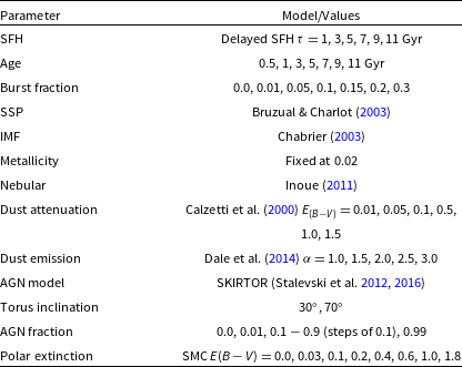


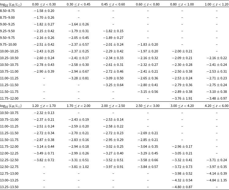


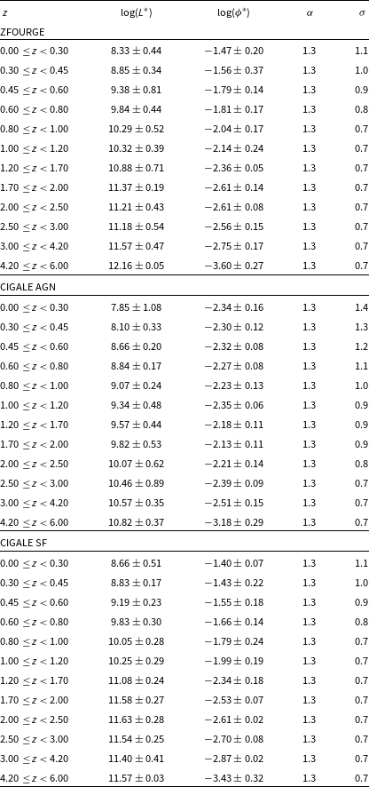


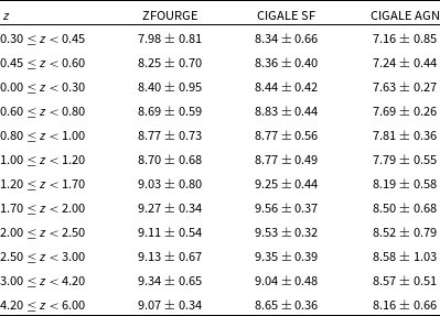


 Open access