


Introduction
Glacier mass loss is accelerating with the changing climate (Hugonnet and others, Reference Hugonnet2021; Bevington and Menounos, Reference Bevington and Menounos2022; Rounce and others, Reference Rounce2023), making glacier projections essential for planning for sea-level rise and changing water resources. Most large-scale glacier models estimate melt using an empirical relationship with temperature (i.e. temperature-index models) (e.g. Marzeion and others, Reference Marzeion2020); however, such models assume a temporally constant degree-day factor over snow and ice surfaces, which is known to vary on subseasonal (e.g. Kuusisto, Reference Kuusisto1980; Braithwaite, Reference Braithwaite1995; Hock, Reference Hock2003) and decadal timescales (e.g. Huss and others, Reference Huss, Funk and Ohmura2009; Matthews and Hodgkins, Reference Matthews and Hodgkins2016). Using temperature as a proxy for energy-balance interactions potentially causes temperature-index models to be overly sensitive to temperature changes (Pellicciotti and others, Reference Pellicciotti, Brock, Strasser, Burlando, Funk and Corripio2005; Gabbi and others, Reference Gabbi, Carenzo, Pellicciotti, Bauder and Funk2014; Marzeion and others, Reference Marzeion2020; Bolibar and others, Reference Bolibar, Rabatel, Gouttevin, Zekollari and Galiez2022). Energy-balance models estimate melt by resolving each individual energy flux, avoiding the assumption that melt scales linearly with temperature (Hock and others, Reference Hock, Radić and Woul2007; Ismail and others, Reference Ismail, Bogacki, Disse, Schäfer and Kirschbauer2023). While their physics-based nature makes energy-balance models more robust to overfitting and thus more transferable than simplified models (MacDougall and others, Reference MacDougall, Wheler and Flowers2011), site-specific calibration is often still necessary to match observations, especially when quality forcing data from local weather stations are not available (e.g. Réveillet and others, Reference Réveillet2018; Temme and others, Reference Temme2023). Given the scarcity of meteorological and mass-balance data on glaciers, rigorous evaluation and continued development of energy-balance models are essential for their reliable application at large scales.
The dominant source of energy for melt on most glaciers is incoming shortwave radiation (e.g. Braithwaite, Reference Braithwaite1995; Pellicciotti and others, Reference Pellicciotti, Brock, Strasser, Burlando, Funk and Corripio2005), making albedo a critical control on melt. Albedo has a complex relationship with melt due to multiple feedback loops involving meteorological variables, such as increasing temperatures diminishing the frequency of summer snowfall events (Johnson and Rupper, Reference Johnson and Rupper2020; Marshall and Miller, Reference Marshall and Miller2020; Ing and others, Reference Ing, Ely, Jones and Davies2025). Current state-of-the-art glacier energy-balance models use various empirical representations of albedo evolution (Brock and others, Reference Brock, Willis and Sharp2000), such as exponential decay over time (Sauter and others, Reference Sauter, Arndt and Schneider2020) or an empirical relationship with another snow property like density (Shannon and others, Reference Shannon2019) or positive degree days (Hirose and Marshall, Reference Hirose and Marshall2013). Calibration of these empirical constants implicitly accounts for several mechanisms of albedo decay, such as surface darkening by light-absorbing particles and snow grain growth. However, the drivers of these mechanisms are changing, such as wildfires occurring with increasing frequency, and these empirical relationships fail to capture the associated albedo feedback loops (Menounos and others, Reference Menounos, Huss, Marshall, Ednie, Florentine and Hartl2025; Williamson and others, Reference Williamson, Marshall and Menounos2025). A more physical implementation of snow evolution considering snow grain growth and deposition of light-absorbing particles, such as that applied in the Community Land Model (Lawrence and others, Reference Lawrence2011), is necessary to capture such dynamic changes. Despite enabling more flexible usage and potentially reducing the number of calibrated parameters, few models apply such physics-based representations of albedo. Thus, we seek to implement and test a physical representation of albedo evolution in a glacier energy-balance model to improve our predictive capabilities.
The most significant challenge with energy-balance models is the considerable data requirements. While temperature-index models only need air temperature to estimate melt, surface energy-balance models require high-quality meteorological forcing data (e.g. temperature, wind speed, relative humidity) to accurately represent heat and mass transfer. These additional meteorological fields increase data requirements and are more challenging to interpolate spatially than air temperature (e.g. Risk and James, Reference Risk and James2022). Energy-balance models are thus often forced by observations from on-ice or glacier-adjacent automatic weather stations (e.g. Fitzpatrick and others, Reference Fitzpatrick, Radić and Menounos2017; Hill and others, Reference Hill, Dow, Bash and Copland2021; Conway and others, Reference Conway2022; Abrahim and others, Reference Abrahim, Cullen, Conway and Sirguey2023). However, in situ forcing data limit applications to glaciers where observations are collected. Alternatively, gridded reanalysis datasets enable large-scale applications (e.g. Shannon and others, Reference Shannon2019) but introduce biases due to their low spatial resolution and must be downscaled to the glacier scale.
The complexity of downscaling varies from simple elevation-based scaling (e.g. temperature lapse rates) to statistical methods like bias corrections using in situ data (e.g. quantile mapping) to more sophisticated dynamical downscaling, such as using the Weather and Research Forecasting model (e.g. Draeger and others, Reference Draeger, Radić, White and Tessema2024). When using statistically downscaled reanalysis data, calibrated parameters are still needed to further correct model biases (e.g. Réveillet and others, Reference Réveillet2018; Temme and others, Reference Temme2023), which improve the fit to observations but limit the model’s applicability to the site(s) where it was calibrated or those with similar characteristics. Dynamical downscaling eliminates the need for calibrated parameters and thus is more transferable to non-monitored sites; however, it increases computational expense and does not remove the in situ data requirement for validation (Arndt and others, Reference Arndt, Scherer and Schneider2021; Draeger and others, Reference Draeger, Radić, White and Tessema2024). While dynamically downscaled data products are readily available for certain geographic regions (e.g. Lader and others, Reference Lader, Bidlack, Walsh, Bhatt and Bieniek2020; Spero and others, Reference Spero2025), no equivalent product exists for a majority of Alaska’s glaciated area, and the lack of high-elevation meteorological observations presents a major challenge in the development and validation of such a product. Thus, more research is needed to evaluate the limitations of statistically downscaled reanalysis data in forcing glacier energy-balance models.
Energy-balance models require both physically based parameters (e.g. temperature lapse rate, bare ice albedo) that are measurable but often unmeasured, and empirical parameters (e.g. stability correction for turbulent fluxes, snow densification) that were calibrated to other glaciers. Both types of parameters are poorly constrained and must be calibrated or assumed, which introduces uncertainty as to whether they represent physical reality or compensate for other forcing or model biases. Some energy-balance model studies ignore this parameter uncertainty, which may be justified in the case of high-quality forcing data (e.g. Marshall and Miller, Reference Marshall and Miller2020; Hill and others, Reference Hill, Dow, Bash and Copland2021; Pradhananga and Pomeroy, Reference Pradhananga and Pomeroy2022), while more robust studies use sensitivity analyses and/or ensembles to assess parameter uncertainty (e.g. Réveillet and others, Reference Réveillet2018; Ing and others, Reference Ing, Ely, Jones and Davies2025; Phelps and others, Reference Phelps, Radić and Williamson2025). Sensitivity analyses can justify the use of assumed values by identifying parameters with minimal influence on model output, enabling constant values to be applied where appropriate (e.g. Klok and Oerlemans, Reference Klok and Oerlemans2002; Réveillet and others, Reference Réveillet2018; Arndt and others, Reference Arndt, Scherer and Schneider2021). Alternatively, ensembles of parameters can be used to quantify uncertainties for physically or empirically based ranges of parameters (e.g. Mölg and others, Reference Mölg, Maussion, Yang and Scherer2012; Ismail and others, Reference Ismail, Bogacki, Disse, Schäfer and Kirschbauer2023). While both approaches help quantify uncertainty, calibration to limited datasets can still lead to overfitting and poor transferability (Prinz and others, Reference Prinz, Nicholson, Mölg, Gurgiser and Kaser2016; Temme and others, Reference Temme2023). The most robust assessment of parameter uncertainty incorporates diverse datasets and applies multi-objective optimization methods (Rye and others, Reference Rye, Arnold, Willis and Kohler2010; Zolles and others, Reference Zolles, Maussion, Galos, Gurgiser and Nicholson2019).
We developed a new open-source glacier energy and mass-balance model specifically designed to run on broadly available forcing data and incorporate robust calibration procedures. We call this the Python Energy Balance model for Snow and Ice (PEBSI), which improves upon existing snow albedo frameworks by coupling with the Snow, Ice and Aerosol Radiative (SNICAR) model (Flanner and others, Reference Flanner2021; Whicker and others, Reference Whicker, Flanner, Dang, Zender, Cook and Gardner2022). This study leverages extensive field observations at Gulkana Glacier, including long-term records of seasonal mass balance and snow density, as well as on-ice meteorology and daily surface-height change measurements from the 2024 melt season, to force, calibrate and evaluate the model. We assess the viability of forcing the model with statistically downscaled climate reanalysis data and examine the tradeoffs when calibrating parameters to multiple in situ datasets. Our work ultimately aims to provide a framework for assessing model performance across multiple objectives and discusses the challenges of forcing and calibrating glacier energy-balance models in data-scarce environments.
Field data
Gulkana Glacier, or C’ulc’ena’ Łuu’ (cutting stream glacier) in the Ahtna language, is a temperate mountain glacier (∼15.5 km2 in 2021) located in the Alaska Range that has a robust history of glaciological and meteorological measurements from the U.S. Geological Survey (USGS) Benchmark Glacier Project since 1966 (U.S. Geological Survey Glacier Project, 2016, 2019b). The USGS monitors seasonal mass balance at several sites using traditional stake surveying and snow pit methods on dates near the end-of-winter and end-of-summer. The survey sites range from the lower ablation area (Site A at 1315 m a.s.l.; average annual mass balance of −3.55 m w.e.) to the accumulation area (Site T at 1877 m a.s.l.; average annual mass balance of +0.32 m w.e.) (Fig. 1). Sites B and D have a continuous record of seasonal mass-balance measurements over the 2000–24 study period. Site A was only surveyed through 2014 due to terminus retreat, and a new Site AU was established in 2012. From 2000 to 2024, the average glacier-wide summer and winter mass balance were around −1.7 and 1.0 m water equivalent (w.e.), respectively (U.S. Geological Survey Glacier Project, 2016). The USGS also maintained multiple weather stations adjacent to the glacier which operated year-round with minimal data gaps. One station was located on a lateral moraine on the east side of the lower glacier and operated from 1996 to 2022. A second weather station on a nunatak near the center of the glacier was added in 2012 and is currently maintained (U.S. Geological Survey Glacier Project, 2019b).
Overview of Gulkana Glacier showing the locations of mass balance and meteorological measurements. The inset shows the glacier location in Alaska. The glacier outline from 2021 is overlaid on a WorldView orthophoto from 30 August 2016 (U.S. Geological Survey Glacier Project, 2019a). Data and site locations can be found in Wilson and others (Reference Wilson2025).

In addition to USGS’ seasonal mass-balance and meteorological measurements, we installed instruments to measure the daily surface-height change and on-ice meteorology from 17 April to 20 August 2024. Six GNSS systems were installed on monitored, banded ablation stakes at different elevations on the glacier, and daily surface-height change from interferometric reflectometry was used to estimate climatic mass balance (Wells and others, Reference Wells2024). An on-ice weather station (Fig. S1) measured air temperature, relative humidity, surface pressure, wind speed, and incoming and outgoing shortwave radiation every 15 min which were then averaged to hourly data (Table 1). The on-ice station was floating such that it lowered as the snow melted until it rested on ice, allowing the sensors to remain at an approximately constant height above the surface.
Sensors installed on the on-ice and nunatak weather stations.

Additional measurements of snow properties were made to initialize and validate the model. Snow density measurements were made by sampling 10 cm vertical sections with a 1000 cc wedge cutter throughout snow pits at each USGS site during each end-of-winter field campaign (U.S. Geological Survey Glacier Project, 2016). One snow temperature profile was recorded at Site B using five iButton temperature sensors (precision of ±0.5°C) that were installed at evenly spaced depths (65 cm increments). Concentrations of dust and black carbon were measured from snow samples that were collected at 3 cm increments from the snow surface to a depth of 12 cm at Site D in August with duplicates of the surface. The samples were kept cold in transit to the Snow HydRO Lab at the University of Utah (Salt Lake City) where concentrations of dust and black carbon were quantified using the gravimetric method and a Single Particle Soot Photometer, respectively (Skiles and Painter, Reference Skiles and Painter2017). Additionally, spectral albedo measurements were collected using an ASD, Inc. (Boulder, CO) FieldSpec4 High-Res spectroradiometer (350–2500 nm) and cosine receptor foreoptic on aged snow and bare ice in June 2024.
Meteorological forcing
The model is forced with both reanalysis and in situ meteorological datasets to evaluate the impact of the forcing data on model performance. Following data availability, simulations with MERRA-2 reanalysis data (Gelaro and others, Reference Gelaro2017) are performed for a 25 year period (April 2000 to August 2024), while the in situ data are used to force a single-summer simulation (April to August 2024). For simulations using weather station data, the on-ice station data are used except for incoming longwave radiation, which, due to sensor failure on the on-ice station, is taken from the nunatak station. Because the nunatak station is on an exposed ridge at a similar elevation (1725 m a.s.l.) to the on-ice weather station (1682 m a.s.l.), we expect the incoming longwave measurements to transfer well to the on-ice weather station site. Effects of tilting on shortwave radiation are neglected because the station was observed to tilt less than 3° during deployment. Because no measurements exist to assess these assumptions, we proceed with the uncorrected shortwave and longwave measurements.
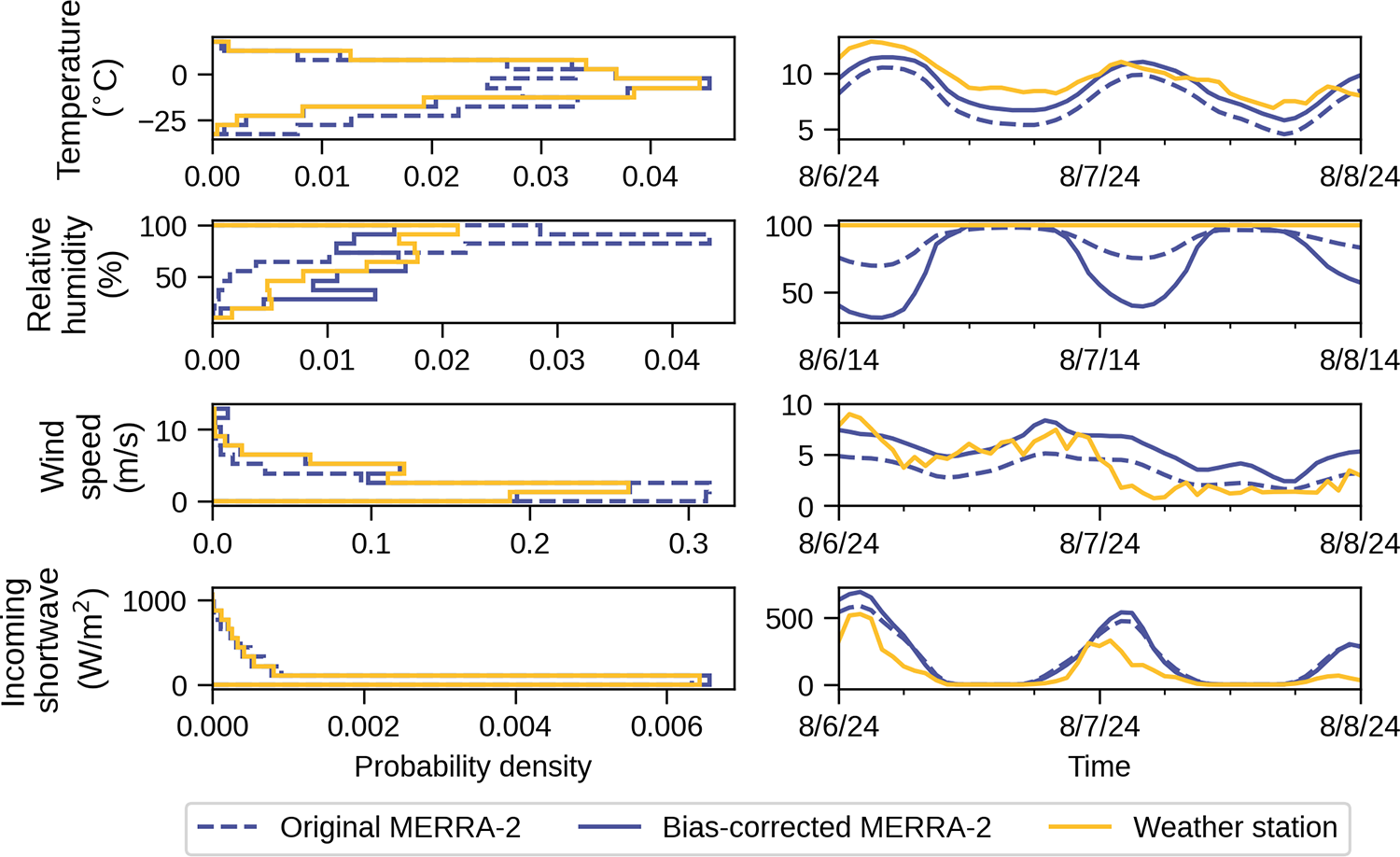
Meteorological variables before and after correction with quantile mapping compared to the distribution of observations from the weather station. Two-day example time series are included in the right column to illustrate the effect of quantile mapping on the actual forcing data. The example time series for relative humidity is taken from a different year than the other variables because relative humidity is not measured at the nunatak station and is thus taken from the moraine station. Note that the distributions of bias-corrected MERRA-2 and weather station data are not perfectly aligned because the bias correction is applied to the entire time series, rather than the temporal subset used to determine the quantile mapping.

Meteorological forcing requirements for the model include all variables listed in Table 1, which are taken either from the automatic weather station (single-summer simulations) or MERRA-2 (25 year simulations), as well as the rate of precipitation and deposition of light-absorbing particles, which are taken from MERRA-2 in all simulations. MERRA-2 is chosen over other reanalysis products, such as ERA-5 (Hersbach and others, Reference Hersbach2020), because it produces deposition fluxes for light-absorbing particles. The MERRA-2 data come from four datasets: surface pressure, 2 meter air temperature, 2 meter eastward and northward wind speed and 2 meter specific humidity from the Single-Level Diagnostics dataset (Global Modeling and Assimilation Office (GMAO), 2015d); incoming shortwave and longwave radiation and total cloud cover from the Radiation Diagnostics dataset (GMAO, 2015c); precipitation from the Surface Flux Diagnostics dataset (GMAO, 2015b); and light-absorbing particle deposition from the Aerosol Diagnostics (extended) dataset (GMAO, 2015a). To limit data requirements, deposition forcing comes from a single representative species of each particle type (i.e. size bin #3 for dust and the hydrophilic species for black and organic carbon) and is scaled to estimate total dry and wet deposition rates (Supplemental Text S2.1; Table S3). The time-averaged size distribution of dust particles is preserved by interpolating mass percentages from the MERRA-2 size bins to the SNICAR size bins (Fig. S2).
The MERRA-2 data are taken from the nearest grid cell, which is centered at 63.5° N, 145.625° W (∼25 km away from the glacier center point) and has 23.3% glacier cover (the remaining area is mixed tundra and boreal forest) and a nominal elevation of 1232 m a.s.l. Temperature and surface pressure are adjusted to the elevation of each site using a constant temperature lapse rate (−6.5 K km−1) and the barometric formula, respectively. Precipitation data are scaled using a calibrated, constant precipitation factor and a precipitation gradient that is applied from the median glacier elevation to the elevation of each site. The precipitation gradient is 0.00013 m−1 based on a linear regression of winter mass balance and elevation data (Supplemental Text S2.2; U.S. Geological Survey Glacier Project, 2016).
Downscaled MERRA-2 data are inspected for bias using coincident in situ observations. Incoming longwave radiation and surface pressure are found to be unbiased (<10% relative bias) and thus are not corrected. The other biased variables (air temperature, relative humidity, incoming shortwave radiation and wind speed) are corrected using quantile mapping (e.g. Rye and others, Reference Rye, Arnold, Willis and Kohler2010; Gobiet and others, Reference Gobiet, Suklitsch and Heinrich2015), which adjusts the distribution of reanalysis data to match that of observed data. For air temperature, relative humidity and incoming shortwave radiation, the underlying distribution varies seasonally; thus, the year-round nunatak weather station observations are utilized for quantile mapping to ensure a representative distribution was used. Wind speed is corrected by the on-ice observations such that the observed data distribution includes katabatic winds and does not include ridge effects from the nunatak. The resulting bias-corrected distributions have an increase in mean air temperature, wind speed and incoming shortwave radiation, and a decrease in mean relative humidity (Fig. 2). The mean absolute and root mean square error do not always improve after performing this correction because quantile mapping only addresses the magnitude and not the timing of MERRA-2 values (Fig. 2). However, the goal of removing bias is achieved for all four variables (Table S2).
For precipitation, we elect to calibrate the precipitation factor instead of performing a bias correction to weather station data because precipitation measurements are themselves biased (Groisman and Legates, Reference Groisman and Legates1994). The precipitation sensor on the nunatak weather station therefore is only used to determine the lower and upper temperature threshold for liquid and solid precipitation (Supplemental Text S2.3; Fig. S3).
Model description
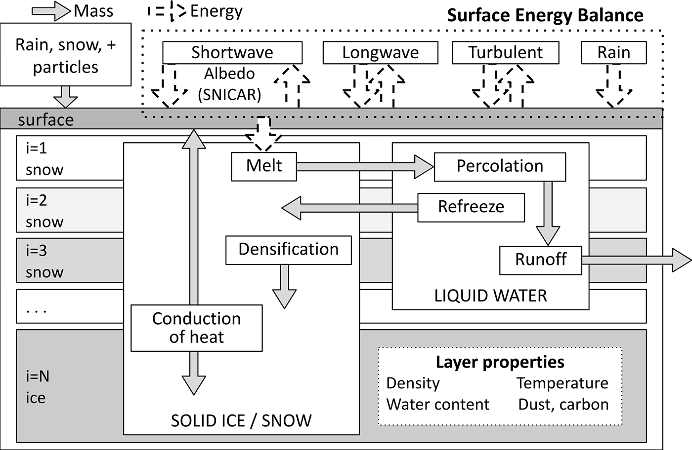
PEBSI simulates the surface energy balance and subsurface mass and energy transfer using a multilayer snow and ice model (Fig. 3) based on well-established methods (e.g. Hock and Holmgren, Reference Hock and Holmgren2005; Sauter and others, Reference Sauter, Arndt and Schneider2020). The model is run at an hourly time step at individual points on the glacier, i.e. lateral heat and mass transfer are neglected. Key details of the model are provided below, and additional details are provided in Supplementary Text S1. All model constants are provided in Table S1.
Schematic of the 1D heat and mass transfer processes included in PEBSI including the surface and subsurface layers.

Surface energy balance
Due to the dependence of multiple energy fluxes on surface temperature, the surface energy balance and surface temperature are calculated iteratively (Eqn (1)):
 \begin{equation}{Q_{\text{m}}} + S{W_{{\text{net}}}} + L{W_{{\text{net}}}} + {Q_{\text{s}}} + {Q_{\text{l}}} + {Q_{\text{r}}} + {Q_{\text{g}}} = 0\end{equation}
where Q m is the melt energy, SW net is the net shortwave radiation, LW net is the net longwave radiation, Q s is the sensible heat flux, Q l is the latent heat flux, Q r is the rain heat flux and Q g is the ground heat flux. The melt energy term can be positive if the surface temperature is at the melting point (0°C); otherwise, the surface temperature is iteratively lowered by 0.25°C increments until the melt energy is within ±0.5 W m−2 of zero or after ten iterations. Incoming shortwave (SW in) and longwave (LW in) fluxes are taken from meteorological forcing and the corresponding outgoing fluxes (SW ref and LW out) are calculated based on the albedo (α) and surface temperature (T s) (Eqns (2) and (Eqns (3):
 \begin{equation}S{W_{{\text{ref}}}} = - S{W_{{\text{in}}}}\alpha \end{equation}
 \begin{equation}L{W_{{\text{out}}}} = - \sigma T_{\text{s}}^4\end{equation}
where σ is the Stefan–Boltzmann constant (5.67 × 10⁻⁸ W m−2 K−4). Incoming shortwave radiation is adjusted to account for topographic shading, terrain-scattered diffuse radiation, and the surface slope and aspect, as described in Supplemental Text S1.
Snow albedo is calculated on a daily time step by the bioSNICAR Python implementation of SNICAR (Cook and others, Reference Cook2020; Flanner and others, Reference Flanner2021; Whicker and others, Reference Whicker, Flanner, Dang, Zender, Cook and Gardner2022). SNICAR simulates the spectral reflectance of a snow column based on optical properties of the layers under diffuse or direct lighting conditions. The snow layer density, grain size and concentration of light-absorbing particles are inputs. Snow grain size evolves based on several processes. First, fresh snow falls at a constant user-specified grain size (54.5 μm; Kuipers Munneke and others, Reference Kuipers Munneke, van den Broeke, Lenaerts, Flanner, Gardner and van de Berg2011). The snow grains age with both dry and wet metamorphosis as parameterized by Flanner and Zender (Reference Flanner and Zender2006). Refrozen grains are assumed to be a constant size of 1.5 mm and the total content of refreeze in each layer is tracked. The grain size of each layer is then calculated by the mass fraction of new, old and refrozen snow. SNICAR is used only for snow layers, while firn and ice albedo are assumed to be constant in time. Firn albedo is a prescribed constant of 0.5, and ice albedo is scaled linearly with elevation between the glacier terminus (0.32, partially debris-covered) and near the end-of-summer snowline (0.49, clean ice). The ice albedo endpoints come from spectrometer and on-ice automatic weather station measurements, and the linear scaling is used to account for the increased presence of debris at lower elevations. The measured reflectance spectrum from the glacier terminus is scaled to the broadband ice albedo at each elevation and used as the underlying surface in SNICAR, which is important when the snow is thin.
Turbulent (sensible and latent) heat fluxes are estimated using Eqns (4) and (5) which apply the bulk aerodynamic formulation (Lettau, Reference Lettau1934; Prandtl, Reference Prandtl and Durand1934) with stability corrections determined from the dimensionless Richardson number (e.g. Essery and others, Reference Essery, Morin, Lejeune and Ménard2013; Radić and others, Reference Radić, Menounos, Shea, Fitzpatrick, Tessema and Déry2017; Sauter and others, Reference Sauter, Arndt and Schneider2020; Lute and others, Reference Lute, Abatzoglou and Link2022):
 \begin{equation}{Q_{\text{s}}} = {\rho _{{\text{air}}}}{c_{p{\text{, air}}}}{C_H}{u_{2{\text{m}}}}\left( {{T_{2{\text{m}}}} - {T_{\text{s}}}} \right)\end{equation}
 \begin{equation}{Q_{\text{l}}} = {\rho _{{\text{air}}}}{L_{\text{v}}}{C_E}{u_{2{\text{m}}}}\left( {{q_{2{\text{m}}}} - {q_{\text{s}}}} \right)\end{equation}
where ρ air is the density of air derived from ideal gas law (kg m−3), c p,air is the specific heat capacity of air (J kg−1 K−1), L v is the latent heat of vaporization or sublimation (J kg−1), u 2m is the 2 meter wind speed (m s−1), T is the temperature (K) and q is the water mixing ratio (unitless). Subscripts ‘2m’ and ‘s’ refer to the 2 meter and surface value for temperature and water mixing ratio. The dimensionless coefficients CH and CE are the Stanton and Dalton number, respectively, which are defined in Supplementary Text S1. Roughness length for momentum is assumed to linearly increase following snowfall events from that of fresh snow to firn (Mölg and others, Reference Mölg, Maussion, Yang and Scherer2012), while ice is assumed to have a constant roughness (Table S1). Roughness lengths for temperature and humidity used in the Richardson stability correction are scaled from the roughness length for momentum by 0.1 and 0.01, respectively (Smeets and van den Broeke, Reference Smeets and van den Broeke2008; Conway and Cullen, Reference Conway and Cullen2013).
Rainfall supplies heat according to the precipitation rate and the temperature difference between the surface and rain (Eqn (6)), assuming the rain is the same temperature as the 2 meter air temperature (Hock and Holmgren, Reference Hock and Holmgren2005):
 \begin{equation}{Q_{\text{r}}} = {c_{p{\text{,w}}}}\left( {{T_{2{\text{m}}}} - {T_{\text{s}}}} \right)P\end{equation}
where P is the rainfall rate (kg m−2 s−1) and cp ,w is the specific heat capacity of water (J kg−1 K−1).
The ground heat flux (Eqn (7)) is estimated from the assumption that all ice layers below 10 m (z temp) remain at 0°C (T temp; Harrison and others, Reference Harrison, Mayo and Trabant1975; Bliss and others, Reference Bliss2020) and transfer heat to the surface based on the temperature gradient (Mölg and Hardy, Reference Mölg and Hardy2004):
 \begin{equation}{Q_{\text{g}}} = \frac{{ - {k_{{\text{ice}}}}\left( {{T_{\text{s}}} - {T_{{\text{temp}}}}} \right)}}{{{z_{{\text{temp}}}}}}\end{equation}
where k ice is the thermal conductivity of ice (W K−1 m−1).
Subsurface layer model
In this implementation, PEBSI is initialized using measurements of snow density and temperature and assumes snow and firn do not contain any light-absorbing particles or liquid water. Melting of snow and ice layers can occur by two methods: surface melt and penetrating shortwave radiation. Surface melt is estimated from the melt energy in Eqn (1) and the latent heat of fusion of ice. Penetrating shortwave radiation can also warm and melt subsurface layers following Bintanja and van den Broeke (Reference Bintanja and van den Broeke1995). Melt and rainwater is then percolated downward based on the porosity of each layer. Following the Community Land Model (Lawrence and others, Reference Lawrence2011), percolation also transports light-absorbing particles through the snowpack. The model tracks changes in dust, black carbon and organic carbon content. These particles are deposited on the top snow or firn layer based on dry and wet deposition rates from MERRA-2, some of which are then flushed through the layers based on the meltwater fluxes and scavenging coefficient of each particle type. Meltwater and the corresponding concentration of light-absorbing particles are assumed to run off-glacier upon reaching the uppermost ice layer.
The meltwater scavenging coefficient, which dictates the amount of each particle type that percolates with meltwater, is difficult to constrain with measurements (Qian and others, Reference Qian, Wang, Zhang, Flanner and Rasch2014) and thus is tuned such that modeled end-of-summer concentrations match measurements from snow samples. For black carbon, the coefficient is determined to be 1. Organic carbon is assumed to have the same scavenging coefficient as black carbon because samples were not analyzed for organic carbon. End-of-summer dust concentrations are found to be consistently underestimated by the model; thus, the value presented in existing literature is used (0.01; Lawrence and others, Reference Lawrence2011). MERRA-2 is unlikely able to capture the magnitude of dust deposition given the presence of local dust sources (Bullard, Reference Bullard2013).
Density of snow and firn layers increases over time from refreezing and densification. Refreezing can occur if liquid water percolates into a layer below the freezing point. The refrozen mass is limited by the availability of liquid water, cold content and pore space. Densification includes the fast settling of fresh snow and slower compression due to overburden pressure following Anderson (Reference Anderson1976) and applied by Sauter and others (Reference Sauter, Arndt and Schneider2020) (Eqns (8– (9):
 \begin{equation}\frac{1}{{{\rho _i}}}\frac{{d{\rho _i}}}{{dt}} = \frac{{{m_{{\text{over}}}}g}}{{{\eta _i}}} + {c_1}{\text{exp}}\left( { - {c_2}\left( {{T_0} - {T_i}} \right)} \right) - {c_3}{\text{max}}\left( {0,\,{\rho _i} - {\rho _0}} \right)\,\end{equation}
 \begin{equation}{\eta _i} = {\eta _0}{\text{exp}}\left( {{c_4}\left( {{T_0} - {T_i}} \right) + {c_5}{\rho _i}} \right)\end{equation}
 where  $\rho$i is the layer density (kg m−3), Ti is the layer temperature (°C), $\rho$0 is the density of fresh snow (kg m−3), T 0 is the melting point temperature (0°C), m over is the overlying mass (kg m−2), g is the gravitational constant (9.81 m s−1), ηi is the layer snow viscosity, and η0 and c 1–5 are constants defined in Table S1. Snow layers are merged into a single firn layer at the end of each summer, which is determined prognostically from the start of accumulation. Firn layers become ice when their density reaches the density of ice (900 kg m−3).
Subsurface heat transfer between layers is modeled assuming one-dimensional heat transfer where the thermal conductivity is a function of each layer’s density following the empirical relationship from Douville and others (Reference Douville, Royer and Mahfouf1995). The surface temperature and temperate ice depth serve as boundary conditions in an explicit, forward-in-time, central-in-space formulation of vertical heat conduction on a layer-centered grid. Numerical stability is ensured by solving the heat conduction equation on a sub-hourly time step according to the Courant–Friedrichs–Lewy condition (Courant and others, Reference Courant, Friedrichs and Lewy1928).
Comparison to in situ observations
USGS provides point stratigraphic measurements in m w.e. for winter and annual mass balance as well as summer accumulation (i.e. new snow that is already present at the end-of-summer date) and winter ablation (i.e. melt that occurred after the previous end-of-summer date). These values are combined to determine the total mass balance between end-of-winter and end-of-summer sample dates. The modeled melt, accumulation and refrozen water between the sample dates is then summed to enable comparison with the measured mass balance. For sites in the accumulation zone, modeled internal accumulation (i.e. refrozen mass below the depth of the end-of-summer surface) is removed because this is not included in the measurement. Comparison to measured snow density requires interpolation of the modeled snow density profile to the measurement depths, while modeled snow depth is directly compared to the measured depth.
Modeled surface-height change is calculated as the combined snow, firn and ice layer height changes due to melt, accumulation and densification and is then compared to daily observations from the 2024 melt season. All observations are representative of the climatic mass balance, i.e. ice dynamics are not considered. Modeled surface-height change is taken only for the relevant vertical section, i.e. densification to the bottom depth of the stake.
Calibration and validation
The model is calibrated using the 25 year simulation compared to four datasets: winter and summer mass balance and end-of-winter snow density and depth. For each of the four datasets, the mean absolute error (MAE) and mean error (bias) are calculated at each of the four sites with long-term seasonal mass-balance measurements (Sites A, AU, B and D; Fig. 1). A grid search is used to inspect tradeoffs with the calibrated parameters and quantify performance with respect to each dataset. To determine which parameters to calibrate, we perform a sensitivity analysis comparing the impact of many parameters on two model variables: mass balance and snow density (Fig. S4). The two most influential parameters are the precipitation factor and the densification parameter which are then calibrated, while default values from the literature are used for all other parameters (Table S1). The precipitation factor scales the amount of accumulation and is varied from 1 to 3 with a step size of 0.25. The densification parameter (c5 in Eqn (9)) impacts the rate of densification and is varied from 0.014 to 0.024 with a step size of 0.002.
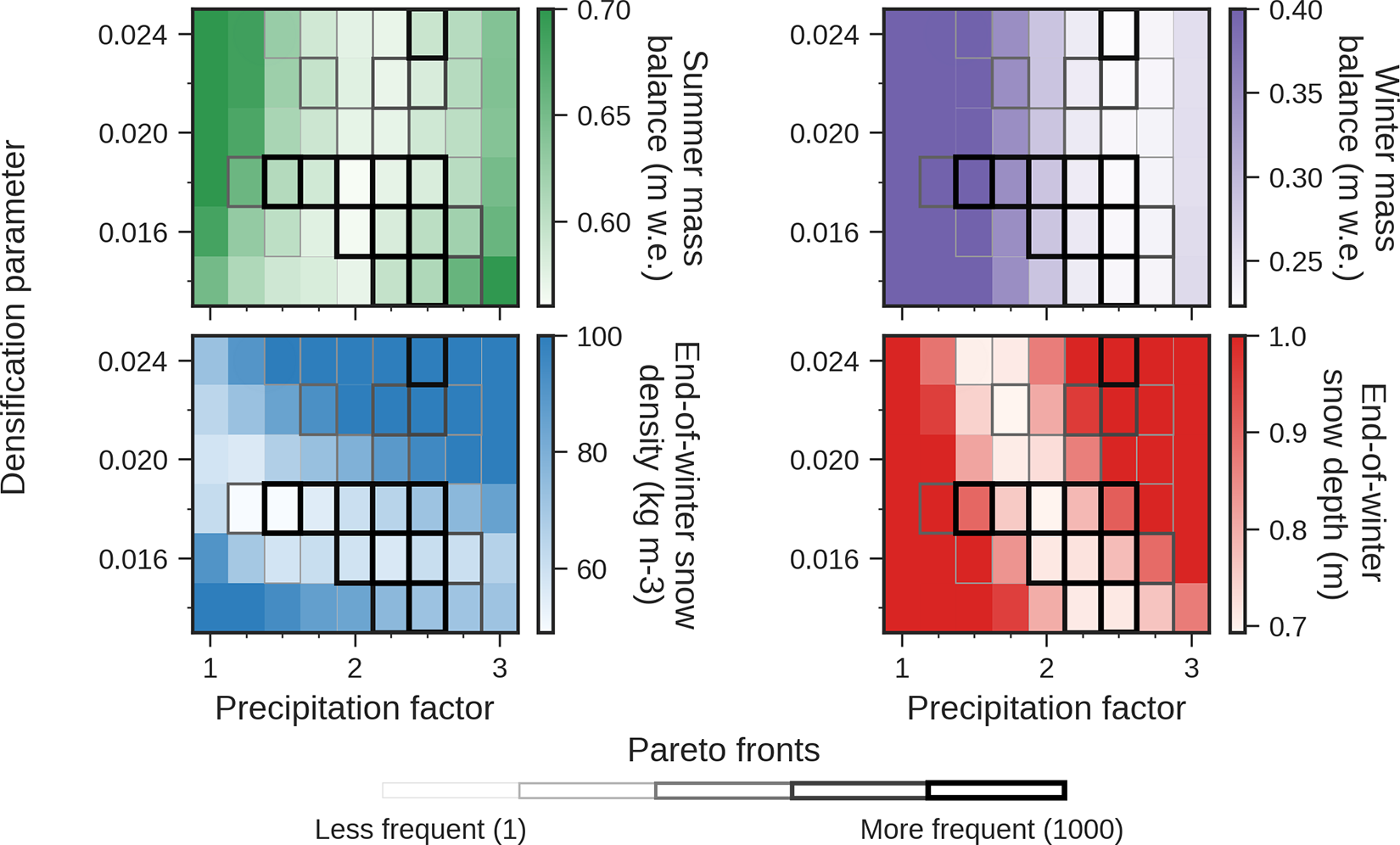
Heatmap of mean absolute error of each dataset on parameter space showing the spread of the Pareto fronts. The optimal solutions for each error metric are shown in white. The grayscale outlined boxes show how many times a parameter set was identified as a Pareto front out of 1000 bootstrapping iterations. Refer to Figure S6 for the heatmap of bias.

The 25 year simulations are split such that 70% of the data are used to calibrate parameters and the remaining 30% are used to evaluate the performance on unseen data. Choosing a distinct calibration and validation period (e.g. 2000–15 for calibration; 2016–24 for validation) results in biased parameters due to underlying temporal trends in the dataset. Thus, we use bootstrapping to randomly divide the modeled and measured mass-balance time series into calibration and validation periods across many iterations, allowing quantification of the uncertainty associated with the choice of years. For each iteration, error metrics for each dataset are calculated for the calibration and validation years and for each parameter combination, then averaged across sites and compared to determine which parameter sets lie on the Pareto front. The Pareto front represents the set of non-dominated solutions, i.e. the combinations across which one objective (e.g. minimizing summer mass-balance error) cannot be improved without worsening the performance of another (e.g. increasing error in snow density or winter mass balance). The Pareto fronts are then aggregated across 1000 iterations to inspect the frequency at which each parameter combination is optimized. The model performance is further evaluated by applying Pareto front parameters to the single-summer simulation at Site B and assessing the error with respect to surface-height change and albedo.
To determine the best overall parameter set, the MAE for each metric is normalized between its minimum value (set to 0) and a maximum cutoff determined from the 75th percentile of the probability distribution function (set to 1). The maximum cutoff is chosen to remove outliers and consider only an acceptable subset of all solutions. Equal weights are applied, and the parameter combination which results in the lowest weighted error is determined. This equal-weighting scheme is used to repeat the calibration for each individual site, and the optimized parameters from each site are used to model the other sites to quantify cross-site parameter transferability.
Results
Calibration and validation on the 25 year simulations
Bootstrapping is used to identify optimal parameters while considering uncertainty in the calibration and validation periods, which eliminates sampling bias (Fig. S5). Pareto fronts are identified which represent non-dominated solutions for each random subset of calibration and validation data. The outlined Pareto front region over each heatmap in Fig. 4 reveals where error is minimized across the four datasets. Overall, winter mass balance is modeled better than summer mass balance with an absolute minimum error of 0.22 and 0.56 m w.e., respectively. The winter mass-balance error is minimized at a precipitation factor of 2.5, indicating that reanalysis data underestimate winter accumulation when left unscaled (Fig. S6). The value of the densification parameter which appears most frequently in Pareto front parameter sets is the default value (c 5 = 0.018), suggesting this empirical relationship transfers well to Gulkana Glacier.
A conflicting trend in performance exists between the summer mass balance and end-of-winter snow density and depth (Fig. S7). As the precipitation factor increases, summer mass-balance performance is improved by increasing the densification parameter, while end-of-winter snow depth and density performance are improved by decreasing the densification parameter. These tradeoffs are important for modelers to recognize and understand when calibrating complex models to limited data, as errors with respect to multiple datasets cannot be simultaneously optimized.
Time series of the observations and differences between modeled quantities and observations from 2000 to 2024 for various values of the densification parameter and precipitation factor. The left column (panels a, d, g and j) shows the measured and modeled time series, where snow density is averaged across the pit depth. Modeled time series in gray use a densification parameter of 0.016 and precipitation factor of 2.25. The center column (panels b, e, h and k) shows the difference between modeled results and data when varying the densification parameter (c 5), and the right column (panels c, f, i and l) shows the difference between modeled result and data when varying the precipitation factor (k p). The other parameter is held constant at the value determined from the equal weighting scheme. In the row labels, b refers to seasonal mass balance with subscript ‘s’ for summer and ‘w’ for winter, ρ refers to end-of-winter bulk snow density and h refers to end-of-winter snow depth. Subscripts ‘mod’ and ‘meas’ refer to modeled and measured quantities, respectively.

To simulate calibration on a more data-scarce glacier, we test how the parameters change when limiting the data to annual or seasonal mass balance (Fig. S8). Removing the snow density and snow depth calibration data eliminates most of the Pareto fronts identified using all four datasets. Most Pareto fronts now occur at high values of the densification parameter, suggesting the snow densification would be underestimated when only mass-balance data are used for calibration (Fig. S6). Further limiting the calibration data to the annual mass balance removes the competition between winter and summer. The range of Pareto fronts is reduced, and the same parameter set is identified for most iterations regardless of the calibration and validation time periods. This parameter combination also lies on the Pareto front when calibrating on all four datasets but results in high snow density and depth error.
Tradeoff analysis for the 25 year simulations
A tradeoff analysis was conducted to quantify how altering the two calibrated model parameters affects the agreement with in situ observations (i.e. the summer and winter mass balance and end-of-winter snow depth and snow density) (Fig. 5). The precipitation factor directly scales the accumulation term of the mass balance and therefore is linearly related to the snow depth and winter mass balance (Fig. S9). For summer mass balance, the effect of the precipitation factor is nonlinear as summer snowfall increases accumulation but reduces melt by increasing the albedo. Snow density is lower with a higher precipitation factor because the snow depth is overestimated, so the snow is lighter at the measurement depths where the modeled values are interpolated.
High values of the densification parameter cause slower densification and thus decrease snow density and increase snow depth (Fig. 5h, k). Slower densification has no impact on the winter mass balance but a small impact on the summer mass balance by increasing melt, which is counterintuitively driven by lower densities leading to lower albedo. The additional pore space from lower snow density allows more water to be retained, amplifying wet grain metamorphism and decreasing albedo. Thus, increasing the densification parameter decreases the summer mass balance (Fig. 5e). More measurements on the relationship between snow density, liquid water content and grain size would improve our mechanistic understanding of these complex interactions.
Calibration by site for the 25 year simulations
To evaluate the spatial transferability of parameters, the model is calibrated to individual sites by minimizing the weighted, normalized error of all four datasets, and the model performance with those parameters is evaluated at all sites (Fig. 6). Predictably, performance declines when the parameters are applied to a different site. For example, when the parameters are tuned to the accumulation area (Site D) where accumulation is high and melt is low, the mass balance in the ablation area (Sites A and AU) is positively biased, and vice versa (Fig. S10).
Heatmap of mean absolute error at each site when calibrated to each site for the four datasets. Parameters are calibrated to the weighted error, and the resulting parameter combinations are used to generate heatmaps for each individual error metric. The dashed line on the diagonal of the weighted error panel represents the minimum weighted error used to determine the parameters for each site. Refer to Figure S10 for bias.

When calibrating to a single site, calibration to Sites AU and B achieves the best performance on the mean of all sites. Likewise, when the model is calibrated to the site-averaged error, the weighted error is low for the middle two sites (0.26 at AU; 0.34 at B) but higher at the uppermost (0.55 at D) and lowermost (0.51 at A) sites (Fig. 6). These results suggest behavior at high or low elevation sites is difficult to capture when calibrating to mean data, potentially due to missing processes such as topographic wind corrections.
Validation on 2024 melt season
The Pareto front parameter sets determined from the 25 year simulation are applied to the 2024 summer using meteorological data from an automatic weather station and compared to measured surface-height change and albedo at Site B (Fig. 7). Error with respect to the albedo and surface-height change decreases for higher precipitation factors (Fig. 7b, d). The model generally overestimates surface lowering, so increasing the precipitation factor helps compensate for this bias by raising the surface height with more snowfall. Increasing the precipitation factor also reduces error in modeled albedo because the additional snow takes longer to melt, thus increasing the accuracy of the modeled date of bare ice exposure (Fig. 7c). There is no clear relationship between either error metric and the densification parameter. With a smaller densification parameter, the surface lowering due to densification is increased, but melting is decreased. Therefore, the relationship between the densification parameter and surface-height change bias inverts between the early summer when densification dominates and late summer when melt dominates. As observed in the 25 year simulations, modeled snow albedo is generally higher with faster densification because dense snow has less pore space to hold liquid water and thus wet grain metamorphosis is reduced.
Modeled surface-height change and broadband albedo over the 2024 melt season compared to observations at Site B. The gray region represents the area between the minimum and maximum of the Pareto front solutions. The black line for ‘best parameters’ refers to the simulation using parameters identified by the equal-weighting scheme. Only the Pareto front parameter sets are included in the tradeoffs panel on the right. The red lines in panel c represent the date when the ice was exposed, as modeled and as observed by a time lapse camera.

Modeled albedo captures several aspects of the subseasonal variation (Fig. 7c). In the early summer, snowfall events frequently ‘reset’ the albedo to ∼0.9. The quality of reanalysis precipitation data is known to be poor, so the exact timing of snowfall events does not always align. Significant albedo reduction is not observed over the melt period before bare ice exposure, suggesting the snow remained relatively clean, even when highly melt-affected in late July. The timing of bare ice exposure is modeled within a few days of the observation. Because bare ice albedo is assumed to be constant, the range of bare ice exposure timing is the greatest source of albedo variability across parameter sets, occurring between July 1 and July 20. This timing has a large impact on the mass balance due to the increased absorption of shortwave radiation on exposed ice.
The coefficient of determination (R 2) for surface-height change ranges from −2.10 to 0.99, indicating a large range in model performance across sites and parameter combinations (Fig. S11). A negative R 2 indicates that the model performs worse than if the mean of the data was used as a constant predictor, whereas an R 2 close to 1 indicates good agreement between the model and measurements. All Pareto front parameter sets applied to Sites ABB and BD result in R 2 > 0.75, and median R 2 at Site B is 0.77. However, surface lowering at sites D and T is mostly overestimated (Fig. S11). Despite poor agreement with surface-height change at the accumulation area sites, the Pareto front region of modeled mass balance for the 2024 period surrounds the observation for most sites where mass balance was measured (Sites B, D and T) (Fig. S12). The mismatch in performance between surface-height change and summer mass balance at Sites D and T indicates an overestimation of surface lowering that is likely caused by densification and not melt. All sites overestimate surface lowering in the early summer (Fig. S11). However, in the ablation area, ice exposure halts the effect of densification mid-summer, whereas densification occurs at the accumulation area sites for the entire summer, compounding error.
Modeled snowpack ripening is compared to snow temperature measurements from the 2024 melt season and reveals that the modelled snowpack reaches 0°C several weeks before the observed snowpack (Fig. 8). While this error suggests the model transfers excessive heat into the snowpack in the early period, the result has a negligible impact on the mass balance since significant melting does not occur in the model until after the sensors indicate the snowpack is ripe.
Modeled snow temperatures (heatmap) compared to snow temperature measurements from iButton temperature sensors. The triangles are located at the depth the sensor was originally buried, and this depth is extrapolated to the date each sensor first measured 0°C.

Comparison of meteorological forcings on summer mass balance
Using the model parameters determined by the equal-weighting scheme, simulations over the 2024 melt season are conducted with forcings from three datasets—MERRA-2, bias-corrected MERRA-2 and on-ice weather station data—to quantify the impact of climate forcing data on the modeled mass balance (Fig. 9). Forcing the model with uncorrected MERRA-2 data causes the model to consistently overestimate summer mass balance across all sites, especially in the ablation area (Sites AU and AB), ranging from +0.16 m w.e. at Site T to +1.48 m w.e. at Site AB. This bias is primarily caused by the underestimation of wind speed and air temperature in MERRA-2 (Fig. 2), which reduces sensible heat fluxes (Fig. S13) and causes an underestimation of melt. The MAE across the five sites when forced with bias-corrected MERRA-2 (0.22 m w.e.) and the weather station (0.17 m w.e.) are much lower than when forced the uncorrected reanalysis forcing (0.75 m w.e.). Bias correction also improves modeled summer mass balance in the 25 year simulations where MAE is reduced from 1.58 to 0.58 m w.e. (Fig. S14), while winter mass balance remains largely unaffected (MAE of 0.26 vs 0.24 m w.e.). Because the dominant mass-balance process over the winter is accumulation, the primary impact of bias correction is a slight reduction in solid precipitation due to increased air temperatures.
Difference in modeled and measured mass balance for the 2024 ablation season when the model is forced with various meteorological datasets.

Discussion
Bias correction of reanalysis data
Our application of PEBSI at Gulkana Glacier illustrates the challenges associated with using reanalysis data to force energy-balance models. While gridded reanalysis data provide the inputs required for energy-balance modeling on glaciers without in situ data, the spatial resolution of reanalysis data and the associated biases remain a major challenge for large-scale applications. Simple elevation-based downscaling (i.e. temperature lapse rates) has been applied on large scales, but the models are subject to biases such as underestimated accumulation (Shannon and others, Reference Shannon2019) or underestimated ablation, as observed in this study (Fig. 9). Attempting to overcome these biases solely with calibrated parameters can lead to nonphysical representations of physical processes, such as a precipitation factor of 0, highlighting the limitations of reanalysis data when the meaningful scale of meteorological variability is smaller than the resolution of the data.
Here we show that bias-correcting the reanalysis forcing data using statistical downscaling, such as quantile mapping, broadly improves model performance; however, the approach does not capture spatial variations across individual glaciers. For example, wind speed is underestimated by MERRA-2 compared to the weather station at Site B (Fig. 2); however, the bias correction reduces performance with respect to 2024 summer mass balance at Site T (Fig. 9), suggesting that wind speeds are lower at Site T than Site B. In this case, other downscaling approaches, such as distributed wind models (e.g. WindMapper; Marsh and others, Reference Marsh, Vionnet and Pomeroy2023), are a logical addition. Conversely, dynamic downscaling may provide better forcings of multiple meteorological variables on the local scale without requiring in situ data but comes with an additional computational expense. Future work should evaluate downscaling approaches and include observations from other glaciers in the subregion to determine how far away in situ measurements can be taken while maintaining good model performance. Regardless, meteorological and in situ mass-balance data are crucial for validation, highlighting the importance of maintaining existing systems and the need to deploy more systems.
Parameter tuning
Even when high-quality forcing data are available, energy-balance models must be calibrated to in situ observations to properly constrain their numerous model parameters. While the incorporation of multiple calibration datasets can help constrain parameters, multiple-objective optimization rarely yields a solution that minimizes all error metrics simultaneously. Ideally, measurements would be available to constrain all of the energy-balance model parameters (such as how we used a measurement of end-of-summer black carbon concentration to constrain the meltwater scavenging coefficient) and their spatial variations across the glacier; however, this is not feasible given the challenges associated with obtaining these data even at well-monitored glaciers like Gulkana Glacier. Nonetheless, in situ observations such as annual and seasonal mass balance are crucial for evaluating model performance. The fact that only 61 reference glaciers have multi-annual seasonal mass-balance measurements (WGMS, 2025) highlights a major challenge for scaling these models. Furthermore, the accuracy of light-absorbing particle deposition rates in MERRA-2 is unknown, and few observations exist to assess the potential biases we introduce by applying these rates on glaciers. Future work should continue to improve and expand in situ measurements, but given the monetary and logistical constraints associated with fieldwork, additional data from remote sensing, such as albedo (e.g. Williamson and others, Reference Williamson, Copland, Thomson and Burgess2020), snowlines (e.g. Aberle and others, Reference Aberle2025) and melt extents (e.g. Scher and others, Reference Scher, Steiner and McDonald2021), should also be incorporated. As these data are used in calibration, the tradeoffs in model performance across datasets and the influence of the selected parameters on modeled quantities should be assessed.
Here, we calibrated a precipitation factor and densification parameter using seasonal mass-balance data, snow depth and snow density profiles, which revealed complex tradeoffs between parameters that also varied by site. While a sensitivity analysis identified the model output was highly sensitive to these parameters (Fig. S4), the parameters also have physical justifications. The precipitation factor scales the accumulation, which is substantially underestimated at Gulkana Glacier like in many mountainous regions (Groisman and Legates, Reference Groisman and Legates1994). The densification parameter controls the rate of densification by adjusting the snow viscosity—a parameter that is not well-constrained and varies in other model studies (Essery and others, Reference Essery, Morin, Lejeune and Ménard2013). Despite having known effects on specific model quantities, the calibration process inevitably leads to these parameters compensating for other model deficiencies introduced by errors in the meteorological forcing or our parameter(ization) choices. To investigate this compensatory behavior, we derived a data-driven precipitation factor (k p = 1.82) by regressing in situ precipitation data against winter mass-balance observations, then compared the adjusted in situ data to MERRA-2 precipitation scaled by the calibrated precipitation factor (k p = 2.25; Supplementary Text S3; Fig. S15). The adjusted MERRA-2 data closely match annual precipitation from the adjusted in situ data (MAE = 0.28 m a−1), indicating that the precipitation factor primarily corrects for precipitation input bias rather than compensating for other model errors.
While the agreement between calibrated and data-derived precipitation factors is encouraging, the lack of compensatory behavior indicates the densification parameter is the sole lever to tune the model’s remaining biases. Indeed, densification is overestimated in the single-summer simulations, suggesting the calibrated value accounts for the densification process itself and for limitations elsewhere in the model. In theory, more parameters could be calibrated, such as the temperature lapse rate which provides a more direct control on melt (Fig. S4); however, in the absence of data that directly constrains individual parameters, the risk of overparameterization and overfitting increases. Regardless, challenges associated with overparameterization and potential overfitting plague all existing glacier mass-balance models (e.g. Rounce and others, Reference Rounce, Khurana, Short, Hock, Shean and Brinkerhoff2020) and thus should not be a reason to avoid efforts to scale energy-balance models. Our work provides a framework for assessing model tradeoffs which is not limited to parameter uncertainty; for example, the framework could be used to examine model performance under varying levels of model complexity. The potential that energy-balance models may be less sensitive to future increases in temperature (e.g. Gabbi and others, Reference Gabbi, Carenzo, Pellicciotti, Bauder and Funk2014; Marzeion and others, Reference Marzeion2020) and their ability to capture complex albedo feedbacks (e.g. Marshall and Miller, Reference Marshall and Miller2020; Ing and others, Reference Ing, Ely, Jones and Davies2025) highlight the importance of continuing to improve energy-balance models and the forcing data needed to support their use.
Conclusions
This study presents the open-source glacier energy-balance model, PEBSI, and evaluates model performance using a rigorous statistical analysis of parameter tradeoffs on multiple datasets. Comparisons of seasonal mass balance forced by different meteorological data reveal the underestimation of wind speed and air temperature in uncorrected MERRA-2 causes the model to underestimate ablation. Bias-correcting the MERRA-2 data improves the simulated summer mass balance, highlighting the importance of in situ meteorological data and the value of automatic weather stations on or near glaciers. The calibrated model was also applied to a single-summer simulation forced with on-ice weather station data and performed well at most sites compared to daily surface-height change and seasonal mass balance. The greatest errors were consistently found at the highest and lowest elevation sites, indicating the model performs best closer to the median glacier elevation where both weather stations were located.
The robust in situ dataset of seasonal mass balance, daily surface-height change and snow density enable comparison of tradeoffs on multiple corresponding modeled quantities. We find that error across all datasets cannot be minimized with a single set of parameters, illustrating shortcomings associated with model overparameterization and forcing data, even for a well-monitored glacier. Acknowledging the potential for overfitting of parameters is important in energy-balance model studies because unaccounted errors can manifest in modeled quantities that were not evaluated, such as snow density. However, these limitations should not preclude the use of energy-balance models in large-scale applications. Here we highlight a framework that can be used to quantify these tradeoffs and sources of uncertainty, opening opportunities for further exploration of model complexity and performance tradeoffs. Future work should assess the performance of climate downscaling methods on reanalysis forcing data and utilize remote sensing products to expand applications of energy-balance models. Furthermore, the albedo framework of PEBSI should be used to investigate how glacier mass balance is impacted by albedo feedbacks, such as those driven by wildfires and heatwaves, to improve our projections of glacier mass change.
Supplementary material
The supplementary material for this article can be found at https://doi.org/10.1017/jog.2026.10154.
Data availability statement
All data used in this study are publicly available. USGS data releases include the seasonal mass balance, snow depth and density (U.S. Geological Survey Glacier Project, 2016), and off-ice weather station data (U.S. Geological Survey Glacier Project, 2019b). On-ice weather station data, daily surface-height change, snow temperature and spectral albedo measurements are available in Wilson and others (Reference Wilson2025). The code and manual for the energy-balance model can be found at https://github.com/clairevwilson/PEBSI/. The version of PEBSI used in this study is archived at https://doi.org/10.5281/zenodo.19099385.
Acknowledgements
This material is based upon work supported by the National Science Foundation (NSF) Graduate Research Fellowship Program under Grant No DGE2140739. Any opinions, findings, and conclusions or recommendations expressed in this material are those of the authors and do not necessarily reflect the views of the National Science Foundation. C.W. and D.R. were supported by the NSF Arctic Natural Sciences grant 2214509. A.W. and D.R. were supported by the National Aeronautics and Space Administration (NASA) award 80NSSC20K1296. S.M.S. was supported by the NASA award 80NSSC22K0686. The Benchmark Glacier Project, including E.B. and L.S., was supported by the U.S. Geological Survey Ecosystems Mission Area Land Change Science Program. Any use of trade, firm or product names is for descriptive purposes only and does not imply endorsement by the U.S. Government. We acknowledge the use of imagery from the Worldview Snapshots application (https://wvs.earthdata.nasa.gov), part of the Earth Science Data and Information System (ESDIS). We appreciate the help from all people involved with the fieldwork, including Marie Schroeder, Zanden Frederick, Katherine Bollen and Janet Curran. Thanks to Mathis Leeman for processing the snow samples. We also thank Hamish Gordon for guidance on the use of reanalysis data.
Author contributions
Programming was done by C.W., D.R. and M.F.; field design and deployment by L.S., D.R., C.W., A.W., S.M.S. and E.B; laboratory analysis by S.M.S.; visualization by C.W.; funding acquisition and project administration by L.S. and D.R.; writing of original draft by C.W; all authors contributed to editing and review.


 Open access