
1. Introduction
Electron cryomicroscopy (cryoEM) of biological structures has grown to become a powerful technique for three-dimensional (3D) structure determination of biological molecules. Figures 1–3 show three recent examples of single particle cryoEM structure determinations that span the range from large highly symmetrical viruses to ribonucleoprotein complexes and membrane proteins. In this review, we discuss progress over the last few years and identify some of the key issues that may be important in producing further improvements over the next few years. In addition to the topics we highlight here, there are other technical developments that have the potential to improve cryoEM. These include the development of phase plates (Danev et al. Reference Danev, Buijsse, Khoshouei, Plitzko and Baumeister2014; Glaeser, Reference Glaeser2013; Murata et al. Reference Murata, Liu, Danev, Jakana, Schmid, King, Nagayama and Chiu2010; Nagayama, Reference Nagayama2014), Cc correctors (Kabius et al. Reference Kabius, Hartel, Haider, Muller, Uhlemann, Loebau, Zach and Rose2009) and cooling to liquid helium temperature (Fujiyoshi, Reference Fujiyoshi1998) provided that the problems of beam-induced movement can be minimised. There are also valuable publications that focus on specific issues, including map validation (Rosenthal & Rubinstein, Reference Rosenthal and Rubinstein2015), specimen preparation (Glaeser et al. Reference Glaeser, Han, Csencsits, Killilea, Pulk and Cate2016; Glaeser, Reference Glaeser2016), electron cryotomography (Gan & Jensen, Reference Gan and Jensen2012; Medalia et al. Reference Medalia, Weber, Frangakis, Nicastro, Gerisch and Baumeister2002) and finally three volumes of Methods in Enzymology covering a wide range of topics in more detail (Volumes 481, 482, 483, published in 2010).
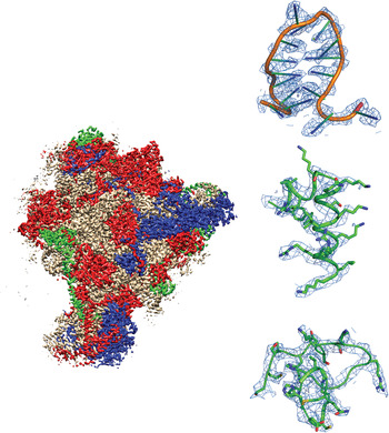
Example of a recently-published single-particle cryoEM structure, with images collected using FEI Falcon direct electron detector – Mitochondrial ribosome, EMDB-2566 (Amunts et al. Reference Amunts, Brown, Toots, Scheres and Ramakrishnan2015). Densities are shown for RNA, an α-helix and a loop.
Example of a recently-published single-particle cryoEM structure, with images collected using Direct Electron DE-12 direct electron detector – Brome mosaic virus, EMDB-6000 (Wang et al. Reference Wang, Hryc, Bammes, Afonine, Jakana, Chen, Liu, Baker, Kao, Ludtke, Schmid, Adams and Chiu2014). Densities are shown for a α-helix and two β-strands.

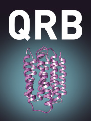
Example of a recently-published single-particle cryoEM structure, with images collected using Gatan K2 Summit direct electron detector – TRPV1 channels, EMDB-5778 (Liao et al. Reference Liao, Cao, Julius and Cheng2013). Densities are shown for three α-helices.

2. Historical overview
CryoEM has drawn strength gradually from a series of contributing ideas and observations, from both academia and industry. These are briefly summarised below.
2.1 The path to CryoEM
Electrons and electron microscopy (EM) have the power to image individual atoms. In the study of inorganic materials, resolutions better than 1 Ångstrom are routinely achieved. However, this requires high-electron doses and Glaeser (Reference Glaeser1971) pointed out that radiation damage by the electron beam meant that structure determination of organic and biological molecules, such as valine and adenine, would require averaging multiple molecular images and suggested that this could be done by recording images from crystals and averaging over many unit cells. Unwin & Henderson determined the 3D structure of bacteriorhodopsin to 7 Å resolution by averaging data from images of unstained 2D crystals of bacteriorhodopsin (purple membrane) at room temperature (Unwin & Henderson, Reference Unwin and Henderson1975; Henderson & Unwin, Reference Henderson and Unwin1975). Taylor & Glaeser (Reference Taylor and Glaeser1974) showed that diffraction patterns and images (Taylor & Glaeser, Reference Taylor and Glaeser1976) of frozen catalase crystals cooled to −120 °C could be recorded with longer exposures than at higher temperatures and would thus give more information due to the reduced effect of radiation damage. In the 1970s, the X-ray crystallographic community also adopted crystal cooling to preserve diffraction from crystals for longer both for small organic molecules and for protein and nucleic acid crystals (Haas & Rossmann, Reference Haas and Rossmann1970; Thomanek et al. Reference Thomanek, Parak, Mossbaue, Formanek, Schwager and Hoppe1973; Petsko, Reference Petsko1975).
The biggest step forward came from the extensive work by Dubochet and his colleagues at European Molecular Biology Laboratory (EMBL) in the early 1980s when they investigated in the electron microscope the properties of thin films of water rapidly frozen at different freezing rates and different temperatures. They characterised vitreous, cubic and hexagonal forms of ice, and developed a simple plunge-freezing method for preparing grids (Adrian et al. Reference Adrian, Dubochet, Lepault and Mcdowall1984; Dubochet et al. Reference Dubochet, Lepault, Freeman, Berriman and Homo1982, Reference Dubochet, Adrian, Teixeira, Alba, Kadiyala, Macfarlane and Angell1984). Their work depended on the development of the first ultra-high vacuum specimen environment in the Philips 400 electron microscope, which had been required by the materials science community to avoid contamination of their clean metallic specimens. Dubochet et al. (Reference Dubochet, Adrian, Chang, Homo, Lepault, Mcdowall and Schultz1988) showed that beautiful images of a whole series of structures from ferritin to adenovirus could be recorded after rapidly freezing EM grids on which thin suspensions of the structures in normal aqueous buffer had been made by application of a small drop followed by blotting and plunge-freezing into liquid ethane. They also developed an efficient double-blade cold shield that they used to protect the grid once it was in the electron microscope and reduce the rate of surface ice contamination from residual water in the microscope chamber.
Freezing and the use of cryoprotection took longer to become widely adopted for X-ray crystallography. It was not until crystals were cooled to near liquid nitrogen temperature that the full benefit of reduced radiation damage was obtained (Henderson, Reference Henderson1990; Hope & Nichols, Reference Hope and Nichols1981; Hope et al. Reference Hope, Frolow, Vonbohlen, Makowski, Kratky, Halfon, Danz, Webster, Bartels, Wittmann and Yonath1989).
2.2 Theoretical background
With some simplifying assumptions, Henderson (Reference Henderson1995) attempted to calculate from first principles the size of the smallest particle that would allow its orientation to be determined from single particle cryoEM images, if perfect images could be obtained that were limited only by the observed radiation damage rates for organic and biological structures in the electron beam. This showed that it should be possible to determine the orientations of single particles as small as 40 kDa and to determine the structure at 3 Å resolution using images of about 12 000 single particles, and less images if the particles had internal symmetry. This calculation was done with the criterion that the structure factors (amplitudes and phases of the Fourier components of the structure) should be recorded with a signal-to-noise ratio of 3. Later Rosenthal & Henderson (Reference Rosenthal and Henderson2003) argued that, since the X-ray protein crystallography community had agreed upon a figure-of-merit of 0.5 as a threshold criterion of structure factor quality, equivalent to a phase error of 60°, the EM community should adopt the same criterion, which translated into a signal-to-noise ratio of 0.6. This 5-fold reduction in the target signal-to-noise ratio reduced the estimate of the number of required single particle images by a factor of 25 to only 600. They also produced a chart that related the number of particles to the achievable resolution, which depended also on the B-factor that could be used to characterise the resolution-dependent fading of the observed Fourier component amplitudes in real images compared with that expected from theory or electron diffraction. In the interim, Glaeser (Reference Glaeser1999) also argued that the 3 sigma criterion was too stringent and estimated ~1400 particles would be required. Of course, these calculations were all approximate and involved a number of simplifying assumptions, but nevertheless they provided a theoretical framework to justify continued efforts to improve the methods being used in practice. Note that the number of particles required is independent of the particle size or molecular weight. For large particles, each single particle image has more contrast than for small particles so fewer images are required to determine the projection structure to a desired accuracy. On the other hand, large particles require more views to sample reciprocal space adequately in three dimensions, according to the πD/d formula of Crowther et al. (Reference Crowther, Derosier and Klug1970), and these two effects cancel out precisely.
2.3 2D-crystalline, helical and single particles with icosahedral symmetry
The poor quality of the electron images of radiation-sensitive organic or biological structures had been noted and quantitative estimates made of the signal loss in images of 2D crystals of paraffin (Henderson & Glaeser, Reference Henderson and Glaeser1985), but good progress with electron crystallography was still possible by averaging the images of many more molecules than suggested by theory. A 3D structure of bacteriorhodopsin at 3.5 Å was obtained by averaging images containing 5 million molecules recorded using film as the detector (Henderson et al. Reference Henderson, Baldwin, Ceska, Zemlin, Beckmann and Downing1990). Similar numbers were needed to determine the structure for 2D crystals of light-harvesting complex (LHC) II (Kuhlbrandt et al. Reference Kuhlbrandt, Wang and Fujiyoshi1994) and αβ-tubulin zinc sheets (Nogales et al. Reference Nogales, Wolf and Downing1998). More recently, following the development of more powerful computer programs that could deal with images of single particles embedded in ice (Spider, Imagic, Electron Micrograph ANalysis (EMAN), Frealign, Xmipp), and faster computational resources that could be parallelised, structures of icosahedral viruses (Grigorieff & Harrison, Reference Grigorieff and Harrison2011) and helically-ordered proteins at resolutions beyond 4 Å (Egelman, Reference Egelman2007) were achieved. However, these still required the averaging of images of millions of asymmetric units, in the same way as had been required for 2D crystals. For example, the structure of aquareovirus (Zhang et al. Reference Zhang, Jin, Fang, Hui and Zhou2010) at 3.3 Å that allowed side chains of phenylalanine, tyrosine and tryptophan to be resolved required 80 000 icosahedral viruses, which for a T = 13 virus represented 60 million asymmetric units. Rotavirus (T = 13) at 3.8 Å also required 10 million asymmetric units (Zhang et al. Reference Zhang, Settembre, Xu, Dormitzer, Bellamy, Harrison and Grigorieff2008).
The structure of helically ordered protein assemblies in bacterial flagella at 4 Å resolution (Yonekura et al. Reference Yonekura, Maki-Yonekura and Namba2003) and of the acetylcholine receptor at a similar resolution (Miyazawa et al. Reference Miyazawa, Fujiyoshi and Unwin2003) were the two earliest helical structures with relatively high resolution maps. CryoEM of helically ordered assemblies is an active research area with many recent structures reported with resolutions close to 3 Å (Egelman, Reference Egelman2015).
2.4 Single particles without symmetry
Early efforts to use EM for structure determination by combining images of single particles recorded at different specimen tilts came from the group of Hoppe. This involved 3D tomographic imaging of specimens that were relatively stable, including carbon films and heavy-metal-stained molecular assemblies such as fatty acid synthetase (Hoppe et al. Reference Hoppe, Schramm, Sturm, Hunsmann and Gassmann1976) or ribosomal subunits (Knauer et al. Reference Knauer, Hegerl and Hoppe1983). Frank continued this tradition and with van Heel introduced multivariate statistical methods that allowed 2D averaging and classification, with an accompanying improvement in signal-to-noise ratio of the averaged 2D images (Frank & van Heel, Reference Frank and van Heel1982; van Heel & Frank, Reference van Heel and Frank1981). The transition from 2D into 3D for single particles without symmetry came with the introduction of angular reconstitution by van Heel (Reference van Heel1987) and the Random Conical Tilt (RCT) method by Radermacher et al. (Reference Radermacher, Wagenknecht, Verschoor and Frank1987), allowing 3D structures to be obtained from non-symmetrical particles. The first cryoEM images of ribosomes in projection came in 1988 (Wagenknecht et al. Reference Wagenknecht, Grassucci and Frank1988b) and in 3D in 1991 (Frank et al. Reference Frank, Penczek, Grassucci and Srivastava1991). Since then, but prior to the introduction of direct electron detectors, many groups in the ribosome community, in an effort to reach higher resolution on specimens with no internal symmetry, started to collect data sets consisting of several million single particle images (Armache et al. Reference Armache, Jarasch, Anger, Villa, Becker, Bhushan, Jossinet, Habeck, Dindar, Franckenberg, Marquez, Mielke, Thomm, Berninghausen, Beatrix, Soding, Westhof, Wilson and Beckmann2010; Fischer et al. Reference Fischer, Konevega, Wintermeyer, Rodnina and Stark2010), but found that resolution was limited by specimen and image quality.
2.5 Electronic detectors based on phosphor/fibre-optic/charge-coupled device (CCD)
The introduction of electronic detectors in the 1990s as a replacement for film (Krivanek & Mooney, Reference Krivanek and Mooney1993) for recording images or electron diffraction patterns (Downing & Hendrickson, Reference Downing and Hendrickson1999; Faruqi et al. Reference Faruqi, Henderson and Subramaniam1999) had both advantages and disadvantages. The advantage was that the microscopist could immediately see the quality of their specimen and thus avoid the long delay between exposure and observing the image that occurred when using film. Film had to be exposed, removed from the microscope, developed, washed, dried, and digitised using a film scanner, though many microscopists became adept at making judgements from images on wet film. The disadvantage was that the first electronic cameras for EM were based on phosphor/fibre-optic/CCD technology, in which the detective quantum efficiency (DQE) was similar to film when used with 80 or 100 keV electrons. At higher voltages, where the microscope resolution, depth-of-focus, aberrations, and beam penetration improve and the undesirable effects of beam-induced specimen charging are less, the DQE of these detectors was actually a lot worse than film. This was especially clear once it became possible to measure the frequency dependence of the DQE (De Ruijter, Reference De Ruijter1995; Meyer & Kirkland, Reference Meyer and Kirkland2000). Typically the DQE of a phosphor/fibre-optic/CCD electron camera operated at 300 keV was 7–10% at half Nyquist resolution, much lower than film, which has a DQE at half Nyquist of 30–35% when using a 7 µm pixel size (McMullan et al. Reference McMullan, Chen, Henderson and Faruqi2009a). As a result, the highest resolution single-particle structures determined prior to 2012 were largely obtained with images recorded on film (Grigorieff & Harrison, Reference Grigorieff and Harrison2011; Zhang et al. Reference Zhang, Jin, Fang, Hui and Zhou2010).
2.6 Computer-based image processing
The computational methods used in single particle cryoEM were initially ad hoc procedures based on the point group symmetry of the particles being studied. The first cryoEM 3D structure of an icosahedral virus (Vogel et al. Reference Vogel, Provencher, Vonbonsdorff, Adrian and Dubochet1986) at 45 Å resolution used special programs written by Provencher & Vogel (Reference Provencher and Vogel1988). The first cryoEM analysis of clathrin cage structures with D6 symmetry (Vigers et al. Reference Vigers, Crowther and Pearse1986) at 45 Å resolution used R-weighted back-projection from a limited number of cryoEM projections plus 6-fold averaging. Although not strictly single particle cryoEM, Lepault & Leonard (Reference Lepault and Leonard1985) published, including correction for the contrast transfer function (CTF), a 3D structure using cryoEM of individual T4 phage tails, which are single helical particles. A more general approach to computation in 3D EM from images of single particles was started by Frank with the SPIDER package (Frank et al. Reference Frank, Shimkin and Dowse1981) and van Heel with the Imagic package (van Heel, Reference van Heel1979; van Heel & Keegstra, Reference van Heel and Keegstra1981). Both were widely used on images of negatively stained specimens during the 1980s, especially as mentioned in Section 2.4, after the introduction of angular reconstitution (van Heel, Reference van Heel1987) and RCT (Radermacher et al. Reference Radermacher, Wagenknecht, Verschoor and Frank1987). The first 3D ribosome structure using cryoEM at 40 Å resolution came in 1991 (Frank et al. Reference Frank, Penczek, Grassucci and Srivastava1991). EMAN (Ludtke et al. Reference Ludtke, Baldwin and Chiu1999; Tang et al. Reference Tang, Peng, Baldwin, Mann, Jiang, Rees and Ludtke2007) and Frealign (Grigorieff, Reference Grigorieff1998, Reference Grigorieff2007) were developed later with explicit treatment of the CTF that would be required to reach high resolution. The first sub-nanometre single particle cryoEM map was obtained by Bottcher et al. (Reference Bottcher, Wynne and Crowther1997) at 7.4 Å resolution and by Conway et al. (Reference Conway, Cheng, Zlotnick, Wingfield, Stahl and Steven1997) for the hepatitis B virus core, and these structures were calculated with icosahedral-specific programs. The cryoEM structure of the E.coli 70S ribosome reached 11.5 Å resolution in the year 2000 (Gabashvili et al. Reference Gabashvili, Agrawal, Spahn, Grassucci, Svergun, Frank and Penczek2000). The introduction of maximum likelihood (ML) methods into EM came with papers showing applications in 2D from Sigworth (Reference Sigworth1998), Scheres et al. (Reference Scheres, Valle, Nunez, Sorzano, Marabini, Herman and Carazo2005) and Zeng et al. (Reference Zeng, Stahlberg and Grigorieff2007). This was adopted by Scheres (Reference Scheres2012) in RELION and most recently by Grigorieff in Frealign (Lyumkis et al. Reference Lyumkis, Brilot, Theobald and Grigorieff2013). There are now many good packages for single particle cryoEM, which include SPARX (Hohn et al. Reference Hohn, Tang, Goodyear, Baldwin, Huang, Penczek, Yang, Glaeser, Adams and Ludtke2007), Simple and Prime (Elmlund & Elmlund, Reference Elmlund and Elmlund2012; Elmlund et al. Reference Elmlund, Elmlund and Bengio2013), BSOFT (Heymann, Reference Heymann2001) and Xmipp (Marabini et al. Reference Marabini, Masegosa, Sanmartin, Marco, Fernandez, Delafraga, Vaquerizo and Carazo1996) as well as those mentioned earlier.
2.7 Field emission guns, column stability and automation
It is illuminating to compare the determination of the structure of adenovirus using cryoEM in 1986 with progress made by 2010. Adrian et al. (Reference Adrian, Dubochet, Lepault and Mcdowall1984) published the first cryoEM images of adenovirus single particles. Vogel et al. (Reference Vogel, Provencher, Vonbonsdorff, Adrian and Dubochet1986) used these images to calculate a map of the structure at 45 Å resolution and Stewart et al. (Reference Stewart, Burnett, Cyrklaff and Fuller1991) improved this to 35 Å. That early work used cryoEM at 100 keV with a tungsten source and home-made cryo-blades to reduce ice contamination. Twenty-five years later, Liu et al. (Reference Liu, Jin, Koh, Atanasov, Schein, Wu and Zhou2010) successfully determined the structure of adenovirus at 3.6 Å resolution. What were the main factors underlying this remarkable improvement? Note that a 10-fold increase in resolution corresponds to a thousand times more information in 3D. Both the earlier and later work used photographic film, so the same medium was used for image recording. In the intervening period, companies such as Philips (subsequently FEI), Hitachi and JEOL had put an enormous amount of development effort into microscope hardware. The key improvements were (a) the introduction of field emission guns (FEGs), which provided a 500-fold increase in brightness that translates into spatial coherence and substantial increase in information transfer at high resolution, (b) the improvement in both column and cold stage stability reducing image drift, (c) the reduction in ice contamination through better vacuum and cryo-shielding, and (d) the increased accelerating voltage from 100 to 300 keV, which reduced the effect of specimen charging, improved the electron-optical performance and gave better depth of focus for thicker specimens like adenovirus. A useful discussion of these factors can be found in Dejong & Vandyck (Reference Dejong and Vandyck1993).
Alongside these hardware improvements, the group at Scripps pursued a major development in automated molecular microscopy with the Leginon system (Carragher et al. Reference Carragher, Kisseberth, Kriegman, Milligan, Potter, Pulokas and Reilein2000; Suloway et al. Reference Suloway, Pulokas, Fellmann, Cheng, Guerra, Quispe, Stagg, Potter and Carragher2005). This enabled thousands of images to be recorded with the microscope under computer control, using grids with a regular array of holes that had been developed by either Quantifoil (Ermantraut et al. Reference Ermantraut, Wohlfart, Schulz and Tichelaar1997, Reference Ermantraut, Wohlfart and Tichelaar1998) or Protochips (Stagg et al. Reference Stagg, Lander, Pulokas, Fellmann, Cheng, Quispe, Mallick, Avila, Carragher and Potter2006). This degree of automation helped to produce larger datasets with more particles, and the resulting increase in data compensated for many other sources of information loss. Most recently, FEI have introduced a commercial package for automated cryoEM called EPU, which is helping to produce larger datasets with less human effort. This greater automation was not available for the adenovirus work by Liu et al. (Reference Liu, Jin, Koh, Atanasov, Schein, Wu and Zhou2010). Those authors simply used more images, collected manually. Whereas the earlier 1991 structure used only 35 adenovirus particles, the later high-resolution structure in 2010 used 45 000 particles from 1350 micrographs. This extraordinary effort shows just how important automation has now become. The same structure determination could now be carried out more quickly and with much less human effort due to automation.
Finally, it is worth mentioning that one product in particular has come to dominate the recent surge in high-resolution structure determinations. That is the FEI Titan Krios, whose platform itself and the associated developments of optics, stage, vacuum system, and autoloader represent an investment of more than $100 M.
3. Recent advances
3.1 Direct electron CMOS detectors
A big step forward came around 2012–2013 with the introduction of direct electron detectors fabricated using complementary metal oxide semiconductor (CMOS) technology that had been developed over the preceding decade (Faruqi et al. Reference Faruqi, Henderson, Pryddetch, Allport and Evans2005; Milazzo et al. Reference Milazzo, Leblanc, Duttweiler, Jin, Bouwer, Peltier, Ellisman, Bieser, Matis, Wieman, Denes, Kleinfelder and Xuong2005). These detectors have a rolling-shutter readout mechanism and can read out images continuously with a frame rate that can range from 1 to 1000 Hz or more. The frame rate simply depends on how many parallel analog-to-digital converter (ADC) are used to digitise the voltage on the diode in each pixel, whose voltage is discharged by electron-hole pairs that are created as the incident high energy electron passes through the detector. The effect of radiation damage on the detector can be minimised both by using special radiation-hard design features, but also by increasing the frame rate, since radiation damage increases the leakage current and this is less important at fast frame rates. In addition, these CMOS detectors can be made to be very thin (by backthinning after wafer fabrication), and this reduces the amount of energy deposited in the incorrect pixel of the detector by electrons backscattered from the substrate material, which also adds noise to the image. The modulation transfer function and DQE of a direct electron detector can be improved by a factor of two or more by backthinning (McMullan et al. Reference McMullan, Faruqi, Henderson, Guerrini, Turchetta, Jacobs and Van Hoften2009c). The reduction of backscattering also results in a 2- to 3-fold improvement in detector lifetime due to reduced overall energy deposition.
The improved DQE, together with the ability to record high frame-rate movies has brought synergistic advantages. The improved DQE alone provides a significant advantage. The availability of movie recording allows the effect of beam-induced specimen movement and image blurring to be reduced by subsequent alignment and appropriate weighting of the individual frames thus increasing the signal-to-noise ratio of the particle images (Bai et al. Reference Bai, Fernandez, McMullan and Scheres2013; Brilot et al. Reference Brilot, Chen, Cheng, Pan, Harrison, Potter, Carragher, Henderson and Grigorieff2012; Campbell et al. Reference Campbell, Cheng, Brilot, Moeller, Lyumkis, Veesler, Pan, Harrison, Potter, Carragher and Grigorieff2012; Grant & Grigorieff, Reference Grant and Grigorieff2015; Li et al. Reference Li, Mooney, Zheng, Booth, Braunfeld, Gubbens, Agard and Cheng2013a; Rubinstein & Brubaker, Reference Rubinstein and Brubaker2015; Scheres, Reference Scheres2014; Vinothkumar et al. Reference Vinothkumar, McMullan and Henderson2014a). These improved motion-corrected images then allow the more accurate determination of the position and orientation of each particle, which produces a 3D map of the structure at higher resolution than it would be without the corrections applied. This higher resolution map then provides a better target for the orientation determination in an iterative manner. Thus the new generation of detectors has arguably produced a bigger impact on the attainable resolution than might have been expected from the increased DQE alone.
3.2 Electron counting
A further improvement in DQE is possible by processing individual frames recorded at very low dose so that single electron events can be identified and their signal replaced either by a delta function at the centroid of the event density at sub-pixel resolution or by applying a more sophisticated procedure (Turchetta, Reference Turchetta1993), before summing the frames to produce a normal image or movie (McMullan et al. Reference McMullan, Clark, Turchetta and Faruqi2009b). Currently the improvement in DQE due to electron counting is most apparent at low resolution (McMullan et al. Reference McMullan, Faruqi, Clare and Henderson2014) and can be exploited by recording images at higher magnification than might normally be chosen and carrying out subsequent 2 × 2 or 3 × 3 binning. At the time of writing this review, only the Gatan K2 camera has a frame rate that is high enough for robust practical recording of images in counting mode (Li et al. Reference Li, Mooney, Zheng, Booth, Braunfeld, Gubbens, Agard and Cheng2013a, Reference Li, Zheng, Egami, Agard and Chengb), though in principle electron counting can be done using any detector with a high enough signal-to-noise ratio.
3.3 Improved computer programs
Many of the early computer programs for image processing required significant experience for successful operation, and compensation for the effects of the CTF were either ignored or involved special procedures with a limited range of applications. EMAN (Ludtke et al. Reference Ludtke, Baldwin and Chiu1999; Tang et al. Reference Tang, Peng, Baldwin, Mann, Jiang, Rees and Ludtke2007) and Frealign (Grigorieff, Reference Grigorieff1998, Reference Grigorieff2007) were the first single particle computational approaches that explicitly included CTF correction at the heart of their operation, which is absolutely required to reach high resolution. The full range of point group symmetries was also embedded in both programs, a feature that had also been available in Imagic since the mid-1980s (van Heel et al. Reference van Heel, Harauz, Orlova, Schmidt and Schatz1996).
RELION was developed by Scheres in 2010 and from the start included a very simple graphical user interface (GUI) that allowed the naïve user to make rapid progress without extensive experience (Scheres, Reference Scheres2012). EMAN had a similar GUI from the beginning, which makes these two systems very popular. RELION also included two significant innovations. A regularised ML scoring system, rather than a simple cross-correlation maximisation algorithm, was used to determine the orientations of the individual single particle images, and to calculate the 3D structures. The ML-scoring itself was not new in RELION. It was also present in Xmipp. However, RELION also used regularisation, which leads to optimal weights on the reconstruction and on the alignments. Parameters for these weights are estimated through the empirical Bayesian approach from the data themselves, rather than through tuning by a user. RELION was also the first approach that forced division of the dataset of individual images into two completely independent halves at the very start of the processing and kept them separate throughout processing. This procedure produced Fourier Shell Correlation (FSC) plots that were termed ‘gold-standard’ following a discussion at a meeting of the EM validation task force (EMVTF) in 2010 (Henderson et al. Reference Henderson, Sali, Baker, Carragher, Devkota, Downing, Egelman, Feng, Frank, Grigorieff, Jiang, Ludtke, Medalia, Penczek, Rosenthal, Rossmann, Schmid, Schroder, Steven, Stokes, Westbrook, Wriggers, Yang, Young, Berman, Chiu, Kleywegt and Lawson2012). The importance of keeping the two halves of any dataset completely separate to avoid ‘overfitting’ of noise had been well established from the work of Grigorieff (Grigorieff, Reference Grigorieff2000; Stewart & Grigorieff, Reference Stewart and Grigorieff2004), but was unpopular because it gave less optimistic (although realistic) resolution estimates. RELION uses the gold-standard FSC curves to estimate the signal level in the dataset of images, to filter the projections used for orientation determination, and to produce 3D maps with more reliable resolution estimates (Scheres & Chen, Reference Scheres and Chen2012). The resolution-limited refinement of particle orientations is also an important principle that can be used to avoid ‘overfitting’ and has always been a recommended feature in Frealign (Grigorieff, Reference Grigorieff2007). Many other improvements in the different packages have been made that are too detailed to be described here. For example, EMAN uses a spectral-signal-to-noise-ratio weighted Fourier Ring Correlation (FRC) integral alongside other similarity metrics for particle registration.
Elmlund introduced SIMPLE (Elmlund & Elmlund, Reference Elmlund and Elmlund2012) and PRIME (Elmlund et al. Reference Elmlund, Elmlund and Bengio2013) with the goal of transforming raw 2D single particle images into an initial model of a 3D structure with no information other than the pixel size and the expected particle size. Although this ignored the CTF completely, which limited the resolution of the resulting structures to around 20 Å, it worked very well on homogeneous datasets.
Three-dimensional classification was originally implemented within Xmipp (Sorzano et al. Reference Sorzano, Marabini, Velazquez-Muriel, Bilbao-Castro, Scheres, Carazo and Pascual-Montano2004) and improved by addition of a ML-scoring system (Scheres et al. Reference Scheres, Valle, Nunez, Sorzano, Marabini, Herman and Carazo2005, Reference Scheres, Gao, Valle, Herman, Eggermont, Frank and Carazo2007a, Reference Scheres, Nunez-Ramirez, Gomez-Llorente, Martin, Eggermont and Carazob). Applied to a pre-existing ribosome dataset, this resulted in identification of two key conformational states showing that the images consisted of a mixture of two principal ribosomal complexes. The major population had tRNA in each of the three A, P and E sites, and the minor population had bound elongation factor EF-G and a single tRNA. Later work with 3D classification in RELION on the same dataset of images, showed the additional presence of about 10% of particles that contained only the large subunit (Scheres, Reference Scheres2012). ML 3D classification has recently also been implemented in Frealign (Lyumkis et al. Reference Lyumkis, Brilot, Theobald and Grigorieff2013) with accompanying improvements in structure quality.
4. Outstanding issues and barriers to progress
4.1 Detector development
Further improvements in detector performance require solving one or two remaining problems. First it is important that detectors should be developed so that their DQE is as close as possible to 100%. This will require universal adoption of electron counting since the distribution of energy deposition when individual electrons pass through any detector is stochastic (Fig. 4) and the so-called Landau distribution (Fig. 5) has a very wide spread. Electron counting can be done on any of the current CMOS detectors but is too slow for normal use unless the frame rate is high. A reasonably high frame rate is already available commercially with the Gatan K2/Summit detector (Li et al. Reference Li, Zheng, Egami, Agard and Cheng2013a). Any implementation of electron counting will benefit from minimising missed or overlapping events, which requires a high signal-to-noise ratio and a high frame rate. Improving the signal-to-noise ratio of the read-out helps to minimise missed events. A larger pixel size would allow the use of a thicker epilayer with a resulting increased signal, and a greater degree of backthinning reduces the incidence of electron tracks, where the incident electron is scattered through 90° and tracks through several pixels. Accurate sub-pixel localisation is incompatible with events that appear as tracks. It should be possible for DQE(0) to approach 100%, and there are reasonable prospects for an increase in DQE(Nyquist) to 80–90%. A very small number of electrons will always be backscattered elastically from the detector surface without depositing any energy. Others may pass through and deposit very little energy so they may remain undetected, unless the epilayer is thick enough to improve signal-to-noise ratio. Others will be scattered sideways (Fig. 6) to leave tracks of deposited energy that contain no high resolution information. Finally, unless the frame rate is very high there will always be the temptation to increase the beam intensity thus increasing the number of overlapping events and reducing the overall DQE.
Single frame image recorded using 300 keV electrons, showing single electron events on an FEI Falcon III detector, with excellent signal-to-noise ratio. Falcon III is a highly backthinned sensor with very low noise level. The single frame shows about 100 000 electron events (i.e. one electron per 150 pixels). This figure is similar to that for Falcon III in Kuijper et al. (Reference Kuijper, Van Hoften, Janssen, Geurink, De Carlo, Vos, Van Duinen, Van Haeringen and Storms2015).

Landau distribution for the single electron events from the image shown in Fig. 4. Single electron events are identified by an initial threshold criterion and then all pixels contributing to each event are added together to determine the total signal from each electron. The Landau plot is the histogram of the single-electron event distribution.

Schematic of 300 keV electron trajectories, reproduced from McMullan et al. (Reference McMullan, Faruqi, Henderson, Guerrini, Turchetta, Jacobs and Van Hoften2009c), showing a Monte Carlo simulation of 300 keV electron tracks in silicon. After backthinning to 35 µm, only those parts of the electron tracks highlighted in red would contribute to the recorded signal. Before backthinning, the additional white tracks would contribute a low-resolution component to the signal together with contributions to the noise at all spatial frequencies. The overall thickness of the silicon in the figure is 350 µm with the 35 µm layer that remains after backthinning shown in grey.

4.2 Beam-induced specimen movement
Although many groups are now obtaining outstanding results with this new generation of CMOS detectors, the number of particles or asymmetric units being used to obtain maps with resolutions in the 3–4 Å region is still in the range of 30 000–500 000, often greater (Vinothkumar, Reference Vinothkumar2015). Thus instead of requiring 10 000x more particles than theory suggests are necessary, which was the situation a few years ago, we now need only 100x more in the best cases. Why are such large numbers of particles still needed? All the groups who have studied the information content in the movie time sequence have noticed that the first few frames, with electron doses of 1–4 el Å−2, contribute much less signal to the final structure than the frames that represent the exposure range from about 5–10 el Å−2 (Allegretti et al. Reference Allegretti, Mills, McMullan, Kühlbrandt and Vonck2014; Grant & Grigorieff, Reference Grant and Grigorieff2015; Liao et al. Reference Liao, Cao, Julius and Cheng2013; Scheres, Reference Scheres2014; Vinothkumar et al. Reference Vinothkumar, McMullan and Henderson2014a). Figure 7 shows some examples of such plots. After an exposure of 10 el Å−2, the signal generally decays as would be expected from the effects of radiation damage, which degrades the structure and replaces it with carbonaceous remains, from which hydrogen and other gases have been released by bond fission.
Plot of the B-factors or signal at 7 Å resolution in typical movie sequences, reproduced from Henderson (Reference Henderson2015) with permission.

Probably the most important outstanding problem in cryoEM is to understand and cure this information loss, which is generally thought to be due to beam-induced specimen movement and charging. Our current understanding of some of the key aspects of single particle cryoEM is summarised first.
Following the preparation of samples for cryoEM using the method of Dubochet et al. (Reference Dubochet, Lepault, Freeman, Berriman and Homo1982,Reference Dubochet, Adrian, Teixeira, Alba, Kadiyala, Macfarlane and Angell1984), we typically apply a small drop (3 µl) of a solution of the biological structure of interest to a holey carbon film on a metal EM grid. This is then blotted for a few seconds (using filter paper) and rapidly frozen by plunging the grid into liquid ethane cooled by liquid nitrogen to a temperature just above the freezing point of liquid ethane (−183 °C). The macromolecular structures of interest are thus suspended in this thin film and can be imaged after transfer at liquid nitrogen temperature into an electron cryomicroscope. There are several steps during the freezing process. During the initial stages of the plunge-freezing, the thin film, which is mostly water, is supercooled by the surrounding ethane sufficiently fast that ice crystals do not have time to nucleate and grow. Instead, the temperature of the thin film rapidly falls to −180 °C, resulting in low-density amorphous ice. Only in regions near the metal grid bars of the EM grid does the temperature fall more slowly due to the thermal inertia of the grid bar, so there is a 3–5 µm wide region near each grid bar where the ice is frequently crystalline. The cooling process produces different volume changes in all three elements of the ‘grid’ structure, namely the metal framework, the support film and the ice.
First the width and spacing of the grid bars, which are normally made from copper or sometimes gold, shrinks by 0.2% as the temperature drops from 4 °C to −180 °C. Second, the carbon film shrinks by much less, since its coefficient of linear expansion is ~10x less than copper. Thus the carbon film develops wrinkles as it cools, often termed cryo-crinkling (Booy & Pawley, Reference Booy and Pawley1993). Its behaviour as a relatively robust, rigid support at room temperature is transformed into that of a fairly floppy support film once cooled to liquid nitrogen temperature (Russo & Passmore, Reference Russo and Passmore2016). Russo & Passmore (Reference Russo and Passmore2014a) have shown that supporting films of pure gold on gold grids do not have this problem so they move much less when irradiated in the electron microscope. Alternatively, tungsten or molybdenum grids can been used, because these metals have a lower linear expansion coefficient and less crinkling (Booy & Pawley, Reference Booy and Pawley1993; Glaeser, Reference Glaeser1992; Vonck, Reference Vonck2000). In contrast to the carbon or gold film, the thin film of buffer with a density of ~1.0 g/cc expands as it is supercooled from 4 °C and continues to expand as it is transformed into amorphous ice, ending up with a density that has dropped to 0.93 g/cc, representing a 2.5% linear expansion (Dubochet et al. Reference Dubochet, Adrian, Chang, Homo, Lepault, Mcdowall and Schultz1988). We believe that these differential changes in volume create stresses in the frozen film of amorphous ice, which are locked into the specimen at least until the electron beam is switched on.
Immediately after an exposure is initiated, the incident electron beam interacts with the specimen and a multitude of complicated processes are initiated. There is radiation damage to the water itself, and this causes movements of every water molecule by ~1 Å rms for every 1 e− Å−2 of electron dose for 300 keV electrons (McMullan et al. Reference McMullan, Vinothkumar and Henderson2015). Thus, after a total dose of 25 e− Å−2 the water molecules have moved on average by ~5 Å. There is radiation damage to the protein that breaks bonds and creates free radicals. The bond breakage produces radiation products such as hydrogen, oxygen, methane and ethane, which are gases at liquid nitrogen temperature (Meents et al. Reference Meents, Gutmann, Wagner and Schulze-Briese2010). Heavier fragments may be retained in a cavity in the specimen near to their original undamaged position. The bond breakage pushes the radiation products apart, for example, from 1.5 Å covalent separation to 3.5 Å van der Waals separation, and thus tends to expand the specimen, increasing the internal pressure. The evaporation of fragments however has the opposite effect, leaving gaps that would tend to collapse the structure. The relative balance between expansion and contraction is not known, but the greater amount of beam-induced specimen motion that is observed at liquid helium temperature, where most fragments – except for hydrogen gas – are solids, supports the idea that radiation damage to proteins and fragment production is a principal cause of beam-induced specimen motion. The increased pressure due to bond breakage also causes doming of the thin films of ice over holes in the supporting carbon film both at liquid nitrogen temperature (Campbell et al. Reference Campbell, Cheng, Brilot, Moeller, Lyumkis, Veesler, Pan, Harrison, Potter, Carragher and Grigorieff2012), and even worse at liquid helium temperature (Wright et al. Reference Wright, Iancu, Tivol and Jensen2006).
The motion of the water molecules during electron irradiation can be deduced from the observation of the strength of Thon rings in images of pure frozen water (McMullan et al. Reference McMullan, Vinothkumar and Henderson2015). This beam-induced fluidity would be expected to allow the amorphous ice to move to relieve any stresses that were introduced during the original plunge-freezing of the specimen, as soon as the electron exposure is initiated. We now have three independent observations that in different ways demonstrate that the first 2–4 e− Å−2 of the electron exposure are particularly important. First, we have the observation through the analysis of movie frames (Fig. 7) that the first few e− Å−2 in any exposure contributes much less information to any structure determination than it should, presumably because of specimen motion or image blurring. Second, from the ice Thon ring measurements, we know that the water molecules themselves move to essentially new, uncorrelated positions at electron doses or 2–4 e− Å−2. Third, the publication by Wright et al. (Reference Wright, Iancu, Tivol and Jensen2006) showed that the broad peak in the electron diffraction pattern of pure amorphous ice after irradiation at liquid helium temperature changes from ~3.7 to ~3.2 Å at electron doses of around 2 e− Å−2. They interpreted this as indicating a change in the density of the ice from low density to high density. Irrespective of whether their interpretation of their observations is correct, the key point is that exposures in the range of 1–2 e− Å−2, at both liquid nitrogen and liquid helium temperatures are sufficient to move water molecules to completely different positions. Several independent observations are thus consistent with a relaxation of the stresses in the amorphous ice structure during exposure to the first few electrons per Å2, explaining why beam-induced specimen motion is worse at the beginning of a normal cryoEM exposure. Of course, the water molecules continue to move randomly during the later frames of a typical cryoEM image, but we hypothesise that the stresses have been relieved by this time and so any beam-induced motion is expected to be less systematic in subsequent frames, as observed. It is unclear whether this early period of stress removal involves only smooth motions or includes random jiggling.
How large is the loss of information from this early image blurring? This can be estimated from the known fading of electron diffraction patterns, such as observed for example with 2D crystals of bacteriorhodopsin. We have replotted the data from Stark et al. (Reference Stark, Zemlin and Boettcher1996) in Fig. 8, together with an extrapolation to 300 keV, using a scattering cross-section for 300 keV electrons that is 60% of that for 120 keV electrons, in proportion to the expected 1/(v 2/c 2) relationship, where v is electron velocity and c is speed of light. Stark et al. (Reference Stark, Zemlin and Boettcher1996) showed that the intensity of diffraction at liquid nitrogen temperature at 3 Å resolution for 120 keV electrons fades to 1% after 3 el Å−2 of exposure. By comparison, the diffraction at 7 Å resolution falls only to 50% of the initial intensity after an exposure of 3 el Å−2 at 120 keV (corresponding to 5 el Å−2 at 300 keV). Thus the 3 Å diffraction fades roughly 6x faster than the 7 Å diffraction, which translates into a B-factor of 90 Å2 for typical exposures. This means that we may be losing only about half of the signal in images at 7–10 Å resolution at present through this beam-induced blurring effect, but as much as 98% of the signal at 3 Å resolution, even after alignment of individual frames. Coincidentally, this rough estimate agrees with the missing factor of 50–100 discussed at the beginning of this section.
Plots showing fading of electron diffraction spots at 7 Å and 3 Å resolution from 2D crystals of bacteriorhodopsin in purple membranes, replotted from Stark et al. (Reference Stark, Zemlin and Boettcher1996), comparing radiation damage at liquid helium and liquid N2 temperatures. Note that the experimental measurements were made using 120 keV electrons. The solid line is the best fit to the experimental data. Since the fading should occur at 1.7x higher electron dose at 300 keV, the dashed line is an extrapolation. Image contrast is reduced for higher energy electrons but the longer exposures that are allowed compensate for the reduced contrast and make the signal-to-noise ratio very similar.

In addition to these physical changes throughout the bulk specimen, the incident electron beam produces surface effects. There is mass loss from the two surfaces of the thin film that consists of hydrogen and oxygen gas that originates from the ice as well as volatised fragments of the protein. The rate of mass loss from the ice does not depend on thickness but is a purely surface effect (Heide, Reference Heide1984), so radiation damage deeper inside the ice film involves recombination and annealing of hydrogen and oxygen-based radiation products.
Secondary electrons are also emitted from of the specimen, causing the illuminated area to become positively charged, especially on protruding regions or contamination where the ice surface is not completely flat. This positive charge on the specimen, if not neutralised by a compensating flow of electrons into the illuminated region, builds up during the exposure and causes either electrostatic lensing (Berriman & Rosenthal, Reference Berriman and Rosenthal2012) that blurs the image (Fig. 9), or a tendency of the specimen physically to explode due to electrostatic repulsion forces.
Effect of paraxial illumination to neutralise positive charge build-up. This illustration of hepatitis B viral core uses the off-axis paraxial charge compensation procedure of Berriman & Rosenthal (Reference Berriman and Rosenthal2012) to reduce specimen charge build-up during exposure of an ice-embedded sample to an electron beam that has a smaller diameter than the hole in the holey carbon film. Panel (a) and (b) show images of the same region, in the absence (a) and presence (b) of the paraxial charge compensation. Panels (c) and (d) show a different area with the first image (c) now in the presence and the second image (d) in the absence of charge compensation. The blurring in (a) and (d) is caused by positive charge build-up. Six off-axis apertures in (b) and (c) illuminate regions of carbon film immediately adjacent to the hole, and these beams are blanked in (a) and (d), as described by Berriman & Rosenthal (Reference Berriman and Rosenthal2012). The diameter of the illuminating beam is ~4000 Å.

There is a final concern. It is possible that microscopic charge fluctuations in ice-embedded specimens (because they are insulators) occur during normal cryoEM imaging conditions and that these fluctuations perturb the image throughout a normal exposure, affecting every frame of the dose-fractionated movie exposure series. This effect can be seen at very large defocus values as the well-known ‘bee-swarm’ effect (Brink et al. Reference Brink, Sherman, Berriman and Chiu1998; Curtis & Ferrier, Reference Curtis and Ferrier1969; Dove, Reference Dove1964). We do not yet have enough quantitative analysis to know how well the experimental image frames compare with those from simulations limited only by radiation damage. Even if the current loss of information during the first few frames could be cured, it is possible that the entire exposure series is affected by microscopic electrostatic charging. If it is a serious factor, then one way round this would be to work at higher accelerating voltage, for example 1 or 3 MeV rather than 300 keV, though there are no modern cryEMs that have such a high operating voltage. The higher voltage would have the additional advantage of larger depth of field corresponding to a lower Ewald sphere curvature.
In summary, single particle cryoEM has already realised some of its potential and can currently be used to analyse structures quite well. However, with further efforts to address outstanding issues, the method should reach its full potential. The impact of these improvements will be to produce improved resolution, lead to a requirement for fewer particles, allow determination of orientations and structures of smaller particles, and allow the dissection of more multiple conformations from images of mixed populations.
4.3 Practical solutions to charging and movement
What can be done to minimise beam-induced specimen movement and charging? There is the possibility of using thicker support films (for example 500 Å thick amorphous carbon) that are still holey or gold films (Meyerson et al. Reference Meyerson, Rao, Kumar, Chittori, Banerjee, Pierson, Mayer and Subramaniam2014; Russo & Passmore, Reference Russo and Passmore2014a, Reference Russo and Passmore2016), which are more stable and electrically conductive than amorphous carbon. Glaeser et al. (Reference Glaeser, McMullan, Faruqi and Henderson2011) showed that images of paraffin on thick continuous carbon supports suffered from much less blurring due to beam-induced movement than on thin carbon supports (Glaeser et al. Reference Glaeser, McMullan, Faruqi and Henderson2011). Gold grids are now available commercially from Quantifoil Micro Tools. There is also a possibility that smaller holes will provide a stronger supporting environment that will constrain any tendency to beam-induced motion. There are also efforts to explore the use of graphene support films (Pantelic et al. Reference Pantelic, Meyer, Kaiser, Baumeister and Plitzko2010; Russo & Passmore, Reference Russo and Passmore2014b; Sader et al. Reference Sader, Stopps, Calder and Rosenthal2013), which could help to screen the incoming electron beam from any changes in internal specimen charge distribution, to supply new electrons to replace those ejected by beam damage and to prevent charge build-up.
Another possibility is to employ the equivalent of spotscan imaging (Bullough & Henderson, Reference Bullough and Henderson1987; Downing, Reference Downing1988, Reference Downing1991), which was used successfully to decrease greatly the extent of beam-induced motion in images of 2D crystals, particularly when the specimen was highly tilted (Henderson et al. Reference Henderson, Baldwin, Ceska, Zemlin, Beckmann and Downing1990). The idea behind spotscan is to illuminate only a small area of the specimen (the ‘spot’), for example a circle of diameter ~1000 Å or smaller, at each moment followed by scanning or stepping the illuminating spot across the specimen to build up a complete image. Only the image of the illuminated region suffers from beam-induced blurring during the recording of the image of that spot and the surrounding unilluminated area acts as a robust anchor to minimise movement. The smaller illuminated diameter due to the small spot results in smaller movements.
For single particle specimens suspended in a thin film of ice this produces a problem that did not occur for 2D crystals supported on a carbon film. The illuminated area gets charged up and the resulting images are badly blurred due to electrostatic lensing. Berriman & Rosenthal (Reference Berriman and Rosenthal2012) developed a method to allow small spot illumination of an ice-embedded specimen that prevents charge build up. They used an off-axis multi-hole condenser aperture to provide paraxial illumination that effectively neutralised the charge on the ice by providing a source of secondary electrons to discharge it. They used up to 6 additional off-axis apertures to illuminate the surrounding carbon film and showed that the degree of specimen charging was greatly reduced. The effect of using the Berriman & Rosenthal procedure is shown in Fig. 9 and may be useful for improving the quality of small spot imaging.
5. Need for affordable cryoEM
The technical details of cryoEM are important and can strongly affect the amount of effort required, the resolution obtained and the ability to resolve multiple states. At present, the performance advantage of ‘high-end’ cryoEM (‘high’ because of the large associated capital and running costs of a 300 keV facility) means that those groups and institutions that have access to the best equipment have an enormous advantage over those without such access. Since an installation with equipment that can deliver the best quality images can cost £5 M with annual running cost including management in the range of ~£250 000, this acts a barrier to providing access for research groups that are not located in a major centre. One solution to the problem would be to provide national (e.g. Saibil et al. (Reference Saibil, Grunewald and Stuart2015) for cryoEM in the UK) or international facilities best illustrated by the success and wide availability of third generation synchrotron sources for X-ray diffraction studies (e.g. ESRF, SPring-8).
The preparation of suitable specimens for cryoEM also requires a lot of preliminary evaluation. Alongside the need for excellent biochemistry, there are many pitfalls along the route to producing a perfect cryoEM grid with a good distribution of single particles that are not denatured at the air–water interface, aggregated, stuck to the support film or suffering from preferential orientations. To overcome this list of typical problems requires (preferably) daily access to a cryoEM facility that is good enough for characterisation of any specimen preparation problems, and for collection of small diagnostic datasets. High electron energy is not necessary in such a diagnostic tool since good images can be obtained at 100 keV. However, the coherence of the electron source makes an enormous difference to the detail visible in the highly defocussed images that are need to observe internal structure in smaller proteins. At present, it is not possible to interpret clearly images of protein assemblies of 150 kDa without the higher defocus that can be used with the much higher coherence of a field emission gun (FEG).
Thus alongside the availability of state-of-the-art ‘high-end’ electron cryomicroscopes, the structural biology field also desperately needs an inexpensive diagnostic cryoEM. Such an instrument is needed for preliminary evaluations, and should be able to achieve good enough resolution (e.g. 4 Å, which is enough to resolve the strands in β-sheets and some side-chain information) to evaluate the intrinsic quality of the specimens once a suitable particle distribution has been obtained. This local characterisation of specimens and grids could then feed into and make the best use of regional, national or international resources where higher resolution cryo-microscopes with greater automation could be available. It is certainly unrealistic to expect every laboratory to be able to afford a state-of-the-art facility, which at present needs to include a 300 keV Krios or similar high-end instrument, plus a direct electron detector and possibly also a zero-loss energy filter.
Given the cost of these higher voltage microscopes (due to the need for X-ray shielding and high voltage power supplies), it would be sensible to aim for a 100 or 120 keV instrument for the general market with a FEG electron source (500x brighter than a tungsten filament) and an efficient inexpensive detector at perhaps one tenth of the cost of the ‘high-end’ instruments.
6. Specimen preparation and gallery of cryoEM images
Single particle cryoEM has become very popular. While many of the recently determined structures have benefitted from years of careful biochemistry, there are also many other projects that are stuck at an earlier stage, often due to problems with biochemistry, or grid preparation alongside evaluation of cryoEM images. The main practical difficulty is to produce an even distribution of single particles without aggregation, suspended in a thin film of amorphous ice and with nearly random orientations so that all views are well represented. To get a good distribution of orientations, it often helps to add small amounts of detergents or explore different treatments of a thin carbon support film onto which the specimen is adsorbed, rather than using holey carbon or gold support films. Initially it is often not known what a particular specimen should look like and experience may be needed to know what to expect. As a result, it is good practice to pick the first set of single particles by hand (Henderson, Reference Henderson2013) rather than by using automated particle-picking procedures. A gallery of typical cryoEM images provides some useful common ground.
We show (Fig. 10) examples of cryoEM images of a series of monodisperse, well-behaved proteins such as a small icosahedral enzyme (1.6 MDa), mitochondrial Complex I (900 kDa), β-galactosidase (450 kDa), catalase (240 kDa), C-reactive protein (124 kDa), haemoglobin (64 kDa), ovalbumin (40 kDa) and lysozyme (14 kDa). All the images in Fig. 10 were taken under very similar conditions, as described in the legend. The smallest of these proteins appear simply as small dark dots without enough information to discern the orientation. As the structures get bigger it is possible to determine orientation, but the current minimum size for reliable orientation determination is in the range 100–200 kDa. Since many people are trying to use cryoEM to analyse the structure of membrane proteins or membrane protein complexes, we also show some images (Fig. 11a and b ) of pure detergent micelles or micellar/tubular structures that are often found after very dilute protein samples containing detergent are concentrated during the final step of purification. These detergent structures may appear alongside images of the desired membrane protein:detergent complex and for smaller membrane proteins are virtually indistinguishable. For completeness, some images of DNA (Fig. 11c ) and lipid vesicles (Fig. 11d ) are also shown. Even with preparations believed to represent pure monodisperse membrane proteins where we hope to see a nice distribution of single particles, cryoEM images often reveal the presence of everything except the one thing that is being looked for. Such images sometimes show features recognisable as detergent micelles, liposomes, aggregated protein and/or DNA impurities, sometimes all in the same image. We hope this gallery will help with the interpretation of sample preparation problems so that appropriate steps can be taken to overcome them. It is also useful to know how many particles should be expected in a typical image, assuming the single particles behave as if in free solution. Figure 12 shows a table of the expected particle density for different sized macromolecular complexes at different concentrations on holey grids. The legend gives some possible explanations for why more or less particles than this are often found.
Gallery of images of various specimens. Scale bars 500 Å. All the images shown in Figs 10 and 11 were taken at similar magnifications (1.75 Å/pixel) either on an FEI Polara or Krios at 3–4 µm defocus, 17 e Å−2 s−1 and 4s exposure. The images were taken on Falcon-II/III detectors, except for the β-galactosidase, which was taken on a K2 detector. (a) Pyruvate dehydrogenase E2CD, MW ~1.6MDa. Specimen prepared by Peter Rosenthal in 2001. 5-fold, 3-fold and 2-fold views are clearly visible. (b) Complex I, MW ~900 kDa (Vinothkumar et al. Reference Vinothkumar, Zhu and Hirst2014b). (c) β-galactosidase, MW ~480 kDa (SigmaAldrich G3153; Chen et al. Reference Chen, McMullan, Faruqi, Murshudov, Short, Scheres and Henderson2013). (d) Human erythrocyte catalase, MW ~240 kDa (SigmaAldrich C3566). The central empty region is where the ice is very thin. Surrounding this is a circle of molecules where the catalase has been squeezed out and may be interacting with the air–water interfaces on both sides of the ice film. Further from the centre of the hole where the ice is thicker, the molecules are in random orientations and, once the ice gets much thicker at the edge of the hole, the molecules are even overlapping. (e) C-reactive protein, MW ~124 kDa pentamer (specimen courtesy of Glenys Tennent and Mark Pepys). Many 5-fold views are clearly visible with side views of the pentamers appearing as double dots or lines. Occasional decamers can be seen where the pentamers dimerise. (f) haemoglobin, MW 64 kDa (SigmaAldrich H7379). (g) ovalbumin, MW ~40 kDa (SigmaAldrich A5503). For these small proteins, the images appear as single dots. (h) lysozyme, MW ~14 kDa (SigmaAldrich L6876). Lysozyme molecules can be seen as individual very small dots, but still well above the noise level.

Gallery of images of detergents, DNA, or lipid vesicles, which are often found in single particle cryoEM before optimisation of specimen preparation. Scale bar 500 Å. (a) DDM (Anatrace) 1%, showing lighter densities in the centre of each detergent micelle. (b) LMNG (Anatrace) 1%, showing aggregation into filamentous cylindrical micellar structures. (c) DNA (genomic DNA from E.coli), showing double-stranded filaments with an occasional hint of the 35 Å major groove periodicity. (d) Small spherical lipid vesicles with a small proportion of bilayer disks. POPC lipids (25 mg ml−1) in chloroform (Avanti polar lipids) were dried under argon and the film resuspended in 1% decyl-maltoside solution to give a final concentration of 5 mg ml−1. For making liposomes, the detergent was dialysed out with buffer exchanged twice over 2 days. The liposome solution was passed through an extruder with a 0.1 µm filter and subsequently used for plunge-freezing.

Expected particle distribution on holey grids. The table lists the expected number of single particles in cryoEM, answering the question ‘Given the concentration of the molecule of interest in mg ml−1 and the molecular weight (MW), how many particles should you see in the image if the frozen specimen has the same concentration of molecules that you expect in free solution?’. The number per μm2 is given, as well as the expected particle separation for 800 Å thick ice. The boxes shown in red represent a distribution that is too dense, those in blue too sparse, and those in green about right. If images for the grid show either many more or many less particles than this, then something unexpected is going on. For example all the particles might be sticking to the carbon (if too few are seen in the holes) or the blotting operation might be concentrating the particles (if there are too many), but many different explanations are possible.

There are a few other issues that occur frequently enough to be worth noting here. Purified proteins are often relatively unstable but the stability can be improved in the presence of 10 or 20% glycerol. Since high glycerol concentrations in the electron beam makes the frozen specimen more susceptible to radiation damage, it is usually wise to change the buffer to a glycerol-free medium immediately before preparing grids using a small spin-column. In a similar vein, salt concentrations above about 0.5 M can increase the background contrast in the image, especially if there is some evaporation during the blotting procedure, so it is best to aim for the lowest salt concentration that is compatible with the stability of the protein or macromolecular complex being investigated. Finally, one unsolved problem concerns the deleterious effect of the air–water interface. During the blotting procedure, the specimen is exposed to the air-water surface on one or both sides of the thin film of buffer for a period of several seconds, depending on whether the drop of specimen solution is adsorbed to a thin continuous carbon film or applied to a holey carbon film. It is well known that proteins are adsorbed and frequently denatured at most surfaces (Ramsden, Reference Ramsden1994), including the air-water surface, and the thickness of the adsorbed layer increases with time. Clearly, it would be advantageous to plunge-freeze the thin film as soon as possible after its formation to minimise the number of times the suspended particles interact with the surface.
7. Conclusion
Apart from the increased cost, further improvements in detector performance will produce virtually painless improvements in the attainable resolution, the amount of effort required or the ability to resolve multiple states using cryoEM. The biggest reward in terms of improved signal in high-resolution images or movies will come if the problem of beam-induced movement and image blurring in the early part of the exposure, corresponding to the first few frames of a movie could be cured. This may require some new approach to specimen preparation such as the use of a thicker support with smaller holes into which the ice-embedded molecules are trapped and frozen. Affordable entry-level instruments and more experience in specimen preparation will also be very useful. Progress may even come from new and unexpected approaches. Whatever happens, it is clear that cryoEM has a promising future.
Acknowledgements
We thank Peter Rosenthal for making the frozen E2CD grid used for Fig. 10a , 15 years ago, Glenys Tennent and Mark Pepys for supplying a sample of human C-reactive protein, and Shaoxia Chen for help and advice. We also thank Tony Crowther, Peter Fruhstorfer, Peter Rosenthal, Nigel Unwin, Sjors Scheres, Chris Russo, Greg McMullan and Steve Ludtke for comments and suggestions to improve the manuscript.


 Open access