


1. Introduction
Dynamic glaciers that flow into lakes and fjords and large mass balance gradients characterise Patagonian icefields (Aniya and others, Reference Aniya, Sato, Naruse, Skvarca and Casassa1997; Lenaerts and others, Reference Lenaerts2014). An extremely large amount of snow accumulates over these icefields (e.g., Shiraiwa and others, Reference Shiraiwa2002; Schwikowski and others, Reference Schwikowski, Schläppi, Santibañez, Rivera and Casassa2013). Surface ablation down-glacier removes a large amount of this snow accumulation (Schaefer and others, Reference Schaefer, Machguth, Falvey and Casassa2013, Reference Schaefer, Machguth, Falvey, Casassa and Rignot2015), and frontal ablation does so in fjords or lakes (Minowa and others, Reference Minowa, Schaefer, Sugiyama, Sakakibara and Skvarca2021). The Patagonian icefields have the fastest mass loss rate in the world (Hugonnet and others, Reference Hugonnet2021). Mass loss from lake-terminating glaciers, which have large ablation areas at lower elevations, dominates the mass loss from the ice fields (Minowa and others, Reference Minowa, Schaefer, Sugiyama, Sakakibara and Skvarca2021). Surface ablation has been studied in the lower ablation areas, and net shortwave radiation and sensible heat flux are the two most important contributors to the surface mass balance (SMB) (Takeuchi and others, Reference Takeuchi, Naruse and Skvarca1996; Stuefer and others, Reference Stuefer, Rott and Skvarca2007; Schaefer and others, Reference Schaefer, Fonseca-Gallardo, Farías-Barahona and Casassa2020; Minowa and others, Reference Minowa, Skvarca and Fujita2022). It is the interannual variability of sensible heat flux which modulates the surface ablation, as demonstrated in a 25-year record of point surface mass and energy balance calculations at Glaciar Perito Moreno in the southern Patagonian icefield (Minowa and others, Reference Minowa, Skvarca and Fujita2022). However, the atmospheric conditions that drive the interannual variation in surface ablation are not well understood.
Several studies discuss the importance of local climate on surface ablation in Patagonian glaciers, such as foehn or katabatic winds (Ohata, Reference Ohata1985; Fukami, Reference Fukami1987; Takeuchi and others, Reference Takeuchi, Naruse and Satow1995; Bravo and others, Reference Bravo2019; Temme and others, Reference Temme, Turton, Mölg and Sauter2020). Two major contributors to foehn are isentropic drawdown by interacting between the topography and air masses or dry and warm air advection due to thermodynamic warming (e.g., Elvidge and Renfrew, Reference Elvidge and Renfrew2016). In the latter case, the ascent of moist air masses on mountain slopes cools the air, leading to condensation and latent heat release. Because precipitation removes the condensed water, the air masses that descend on the lee side of the mountain are dry. Thus, a larger temperature lapse rate causes higher lee-side temperatures. In the former case, upwind of the mountain, cool, moist air can be blocked, allowing potentially warmer, drier air to be advected down the lee slopes isentropically. In the southern Andes, the prevailing moist westerly winds interact with the Andean mountain range and can result in dry and warm air advection due to the adiabatic process of dry air on the eastern side. The warm air temperature and strong wind may increase the sensible heat flux at the ice surface to melt ice (Fukami, Reference Fukami1987; Takeuchi and others, Reference Takeuchi, Naruse and Satow1995; Temme and others, Reference Temme, Turton, Mölg and Sauter2020). Clear sky on the eastern side due to dry air may also result from foehn (Elvidge and Renfrew, Reference Elvidge and Renfrew2016; Temme and others, Reference Temme, Turton, Mölg and Sauter2020), which increases the downward shortwave radiation. While foehn winds increase air temperature down the glacier, katabatic winds cool it. The air mass cools and flows down along the glacier, because of the interaction of the ambient warm air mass with the cold glacier surface (Ohata, Reference Ohata1985; Oerlemans and Grisogono, Reference Oerlemans and Grisogono2002). Katabatic winds can modify the air temperature distribution at the boundary layer between the atmosphere and the glacier, resulting in reduced surface ablation. Therefore, in addition to the relative contribution to energy fluxes, detailed meteorological conditions are critical to develop a better understanding the controlling factors of SMB.
Local-scale climate is also important in distributing air temperature from point data to the entire glacier surface to calculate glacier-wide SMB. This is often achieved by defining the temperature lapse rate (e.g., Hock, Reference Hock2003; Bravo and others, Reference Bravo2019, Reference Bravo, Ross, Quincey, Cisternas and Rivera2021). Recent studies conducted in Patagonia investigated 6-month meteorological records and found a steeper temperature lapse rate in the east (7.2°C km−1) than in the west (5.5°C km−1) (Bravo and others, Reference Bravo2019), resulting in a difference in controls of surface ablation along the west-east transect (Bravo and others, Reference Bravo, Ross, Quincey, Cisternas and Rivera2021). In the summer and autumn of 2016, Patagonia experienced a severe drought (Bravo and others, Reference Bravo2019, Reference Bravo, Ross, Quincey, Cisternas and Rivera2021), which appears to have been caused by large-scale climate variability modulating the strength of westerlies (Garreaud, Reference Garreaud2018). To further understand the processes that control the glacier's SMB, it is necessary to investigate the meteorological records from both local- and large-scale perspectives.
In this study, we aim to further extend the results presented by Minowa and others (Reference Minowa, Skvarca and Fujita2022), henceforth MM22, in order to understand the processes controlling extreme ablation and its interannual variability on a Patagonian glacier. In addition to the meteorological records presented in MM22, we analyse another temperature record from 2003–2020 near the equilibrium line of Glaciar Perito Moreno. We used these datasets to investigate the local-scale climate, including foehn or katabatic winds, to understand their influences on the surface ablation of the glacier. We detect foehn events using an algorithm and comparing them with the meteorological records and the modelled energy and surface mass balances to quantify their influence. The interannual variability of foehn frequency is then compared with indices representing climate anomalies in the southern hemisphere. Our study quantifies the influence of the local climate, particularly foehn winds, on the surface ablation of Glaciar Perito Moreno.
2. Materials and methods
2.1 Meteorological records
A permanent automatic weather station (AWS), EMMO (Estación Meterológica Moreno), has been continuously operating since late 1995, located on the bedrock ~450 m southeast of Glaciar Perito Moreno (Fig. 1d) (Stuefer and others, Reference Stuefer, Rott and Skvarca2007). EMMO measures air temperature, relative humidity, air pressure, downward shortwave radiation, wind speed, and wind direction at 1-h intervals. AWS details are described in previous studies (Stuefer, Reference Stuefer1999; Minowa and others, Reference Minowa, Skvarca and Fujita2022). In addition to EMMO, an air temperature sensor, called EMCE (Estación Meterológica Cervantes), has been continuously operating since 2003, located on the southern flank of the glacier at an elevation of 1260 m a.s.l. (Fig. 1d). The elevation of the temperature sensor is nearly the same as the equilibrium line altitude of Glaciar Perito Moreno as 1170–1230 m a.s.l. (Stuefer and others, Reference Stuefer, Rott and Skvarca2007; De Angelis, Reference De Angelis2014). The sensor is placed 2 m above the ground within a radiation shield, with air temperature is measured every hour. There were some data gaps in 2004, 2006, and 2007 due to logging failures.
(a) Mean sea level pressure (white contours), wind (black vectors), and sea surface temperature (SST, colour coded) of ERA5 reanalysis averaged from 1980–2020. Red dot is the location of Glaciar Perito Moreno. (b) An example of synoptic-scale conditions is shown for a foehn day observed on 3 January 2013 (Fig. 4). (c) Topography map of the study site with the glacier area indicated in light blue. Glaciar Perito Moreno, located in Argentina, is highlighted in light yellow. (d) Location of the weather station (EMMO) (red triangle), temperature stations (red circles), and ablation stakes (black crosses). EMMO and EMCE stand for Estación Meteorológica Moreno and Estación Meteorológica Cervantes, respectively. The background map shows topography with 50-m contour intervals. (e) An oblique view of Glaciar Perito Moreno shows the location of weather stations and ablation stakes. Panels (a), (c) and (d) modified from MM22.

The temperature lapse rate, Γ, was calculated between EMMO and EMCE: Γ ≡ −dT/dz, where T is air temperature and z is the altitude of the station. We define it as positive, except during inversions. We note also that both measurements are not taken on the glacier, but rather beside the glacier. Possible influences on the temperature lapse rate due to the location of the stations are noted in the discussion sections.
2.2 Foehn detection
We analyse hourly meteorological records at EMMO and EMCE from 2003–2020 to identify occurrences of foehn by using air temperature, potential temperature, relative humidity, and wind speed (Fig. 2) based on an algorithm proposed in previous studies (e.g., Cape and others, Reference Cape2015; Temme and others, Reference Temme, Turton, Mölg and Sauter2020; Laffin and others, Reference Laffin2021). The potential temperature θ (K) was calculated as: $\theta = ( T + 273.15) ( P_{0} / P) ^{{R_{\rm d} / C_{\rm p}}}$ , where P 0 is standard atmospheric pressure (1013 hPa), R d is the specific gas constant of dry air (287.03 J kg−1 K−1), C p is the specific heat of dry air at constant pressure (1005 J kg−1 K−1), T is air temperature (°C), and P is atmospheric pressure (hPa).
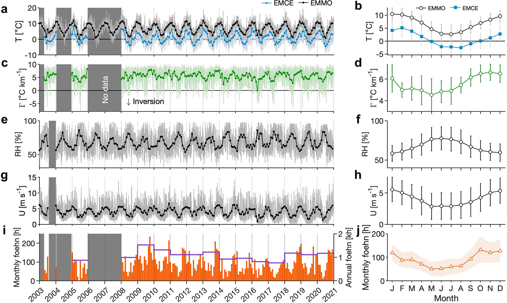
Daily and monthly variables (left panels) and monthly climatology of variables (right panels) observed at EMMO for (a,b) air temperature (T), (c,d) temperature lapse rate between EMMO and EMCE (Γ), (e,f) relative humidity (RH), and (g,h) wind speed (U). The monthly mean air temperature observed at EMCE is also depicted in (a,b). (i) Monthly (orange bars, in hours) and annual (purple line, in kilo-hours) cumulative foehn hours, and (j) monthly climatology of foehn hours. The orange shaded area in panel (j) represents the standard deviation in the mean (1σ). Dark grey shaded areas in the panels indicate periods without any data.
Two requirements must be fulfilled to detect foehn winds: (i) θ EMMO + T ofs > θ EMCE and (ii) 200° < U d < 320°. The potential temperature at the lee station (θ EMMO) must exceed the potential temperature at the mountain station (θ EMCE), which suggests that the air mass warmed adiabatically. We added an offset temperature T ofs = 2.5 K after considering the uncertainty in the estimated potential temperature and sensor accuracy. The threshold in the wind direction (U d) was determined by using the topography at EMMO, in which winds flow from up- to down-glacier (Fig. 1d). In addition to these two requirements, at least one of the following criteria must be met: (iii) $\Delta RH_{\rm EMMO} \ge 14\%$ , (iv) RH < 10th percentile, or (v) RH < 15th percentile and ΔT EMMO ≥ 2.5 K. Here, we define Δ as the difference in the corresponding value over 5 h. The threshold for decreasing relative humidity over 5 h (ΔRH EMMO) was set to 14%, determined by the 90th percentile of the relative humidity reduction over 5 h at EMMO. The 10th and 15th percentiles of relative humidity were 44% and 47% at EMMO. Temperature increases over 5 h (ΔT EMMO) were set to be 90th percentiles of the 5 h temperature increase at EMMO.
To quantify the influence of foehn on the SMB, we calculate the rate of surface ablation during the foehn event. While foehn is detected based on hourly meteorological records, we performed our mass balance calculation using daily time resolution, described in Section 2.3. Therefore, we defined the foehn day to be when the foehn continues ≥10 h over the course of a day. We determine the optimal threshold by calculating the over- and underestimation of surface ablation during the foehn event dependent on the threshold hour (Fig. 11). To do so, we first obtain the frequency of foehn hours (orange stairs in Fig. 11a) and mean surface ablation as a function of the hour (Fig. 11b). By assuming that surface ablation occurs evenly throughout the day, we divide total ablation into ablation during the foehn and not during the foehn (Fig. 11b). We calculate the cumulative effect of foehn events on surface ablation by adjusting the threshold hour. This calculation involves summing the products of the foehn frequency and mean ablation using different threshold hours. When the values are smaller than the threshold, we calculated the sum of products between the foehn frequency and mean ablation during foehn (orange triangle in Fig. 11b), suggesting an underestimation of surface ablation on a foehn day. On the other hand, an overestimation is likely when the sum of products between mean surface ablation not during foehn and foehn frequency is greater than or equal to the given threshold hour (Fig. 11b). We summed the calculated overestimation and underestimation dependent on the threshold hours (Fig. 11c). We find that the 10-h threshold minimises possible errors due to the choice of the threshold hour (Fig. 11c).
2.3 Energy and surface mass balance models
The daily surface mass balance is calculated at stake 1 (S1) in MM22 by quantifying the energy flux for ice melting, snowfall rate, evaporation rate, and the amount of refrozen meltwater. In the calculation, the fluxes directed towards the surface are defined to be positive. The modelled SMB is calibrated and validated with the SMB measured by the ablation stake located at S1. The input data for the models consists of meteorological records obtained at EMMO, with air temperature and relative humidity calibrated against those obtained at S1. The root-mean-square error between the observed and modelled point surface mass balance is 0.69 m w.e. a−1, which corresponds to 4% of the mean annual observed point SMB. Details of the calculation, model sensitivity, and model input are described in MM22.
We need to exercise caution in interpreting net shortwave radiation, net longwave radiation, and latent heat flux over the long-term trend in the SMB (Minowa and others, Reference Minowa, Skvarca and Fujita2022). This is because incoming shortwave radiation and relative humidity sensors may have drifted over the course of the observation period. However, we expect that the influence of the uncertainties in the meteorological observations on the calculated surface and energy balance is limited. The root mean square between the observed and modelled SMB is only improved by 0.03 m w.e. a−1 when we removed the possible drift in incoming shortwave radiation and relative humidity (Minowa and others, Reference Minowa, Skvarca and Fujita2022).
2.4 Climate reanalysis data and climate indices
Monthly ERA5 reanalysis data, made available by the European Centre for Medium-Range Weather Forecasts (Hersbach and others, Reference Hersbach2020), are used to understand how synoptic-scale atmospheric conditions relate to foehn occurrence. We used the 10-m height wind and mean sea level pressure from 1996–2020 over the region 40–110°W and 10–80°S. A seasonal mean anomaly of wind speed and mean sea-level pressure is calculated using mean monthly variables from 1996–2020 during the positive and negative foehn events anomalies.
We use two climate indices that could influence the foehn events at the study site: the Southern Annular Mode (SAM) and the El Niño-Southern Oscillation (ENSO). We utilise the SAM index calculated using the air pressure observed around 40°S and 65°S (Marshall, Reference Marshall2003) (https://climatedataguide.ucar.edu/climate-data/). At both latitudes, the mean zonal sea level pressure is calculated using data from six weather stations. For ENSO, we use the bi-monthly Multivariate ENSO index (MEI.v2) (https://psl.noaa.gov/enso/mei/). The index is obtained by using the empirical orthogonal function of sea level pressure, sea surface temperature, zonal and meridional components of the surface wind, and outgoing longwave radiation over the tropical Pacific between 30°S–30°N and between 100°E–70°W (Wolter and Timlin, Reference Wolter and Timlin2011).
3. Results
3.1 Meteorological records
Figure 2 illustrates the meteorological records since 2003 at EMCE and EMMO. The mean annual temperature at EMCE was 0.82°C, which is 5.89°C lower than that at EMMO (6.71°C). Compared with the temperature observed at EMMO, the maximum temperature at EMCE was recorded a month later, in February (Fig. 2b). The mean annual temperature lapse rate between EMCE and EMMO was 5.6°C km−1, showing large daily and monthly variability (Figs 2c and d). The minimum and maximum daily lapse rates are −7.8°C km−1 and 10.4°C km−1, respectively (Fig. 2c). Temperature inversion is often observed during autumn and winter (Fig. 2c), causing a large seasonality in the monthly lapse rate, ranging from 4.5°C km−1 in May to 6.6°C km−1 in November (Fig. 2d). Lower relative humidity and stronger winds are observed during the more negative lapse rates observed in early austral spring to summer (Figs. 2e–h). These conditions are consistent with foehn characteristics, suggesting higher foehn occurrence in these seasons, which we described in the next section.
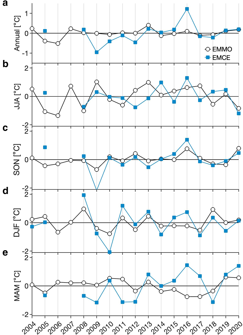
Annual and seasonal air temperature anomalies at EMCE and EMMO are shown in Figure 3. The temperature anomalies are calculated based on the mean temperatures from 2003–2020 for EMCE and 1996–2020 for EMMO. Although both stations are located only 8.5 km apart, their interannual variabilities show a dissimilarity in some years, for example in 2009 and 2016, when we detected the most and the second lowest number of foehn occurrences (Section 3.2). In 2009, the annual air temperature anomaly at EMCE was 0.95°C lower than that at EMMO (Fig. 3a) because of the low-temperature anomalies during SON (September-October-December) and MAM (March-April-May) (Figs. 3c and e). On the other hand, in 2016, the annual air temperature anomaly at EMCE was 1.1°C higher than at EMMO (Fig. 3a). The seasonal mean temperature during MAM in 2016 at EMCE was 2.2°C higher than EMMO (Fig. 3e).
Annual (a) and seasonal (b–e) mean air temperature anomalies observed at EMMO from 1996–2020 (open circles) and at EMCE during 2005, and from 2008–2020 (blue squares). (b) JJA–June-July-August, (c) SON–September-October-November, (d) DJF–December-January-February and (e) MAM–March-April-May.
3.2 Detection and frequency of foehn events
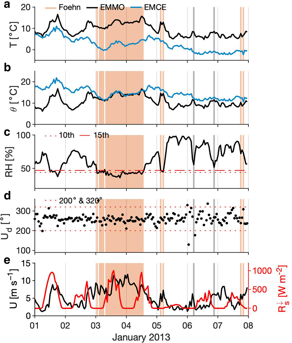
Our meteorological dataset indicates a characteristic foehn signature. Figure 4, for example, shows meteorological records over a week from 1–7 January 2013. Beginning on 3 January 2013, weather conditions with a relatively high temperature, low relative humidity, constant wind direction, and high wind speed are sustained over one and a half days. The potential temperatures calculated at EMMO and EMCE at that time are nearly identical (Fig. 4b) when the foehn event was detected by the algorithm (orange shaded areas in Fig. 4). There are hours when these potential temperatures showed similar values, but they are not determined to be foehn events because of a difference in temperature, relative humidity, or wind direction do not meet the set foehn conditions (grey shaded areas in Fig. 4). To investigate the performance of the algorithm, we conducted a sensitivity test by changing each threshold. We vary ±5th percentiles for temperature and relative humidity, ±0.5°C for offset temperature, and ±1 hour for time difference. The standard deviations of the mean monthly detected foehn hours and total foehn hours were ±11 hours and ±1963 hours, respectively.
A week of hourly meteorological records from 1–7 January 2013. Time series of (a) air temperature (T), (b) potential temperature (θ), (c) relative humidity (RH), (d) wind direction (U d), and (e) wind speed (U) and downward shortwave radiation ($R^{\downarrow }_{s}$ ) (red line). The blue and black lines indicate data obtained at EMMO and EMCE in panels (a) and (b), respectively. Note that only EMMO station data is shown in panels (c)–(e). The vertical light orange hatches indicate periods of foehn events identified by the algorithm. The synoptic-scale conditions on 3 January 2013 are shown in Fig. 1b. The red dotted and dotted-dashed lines in panel (c) indicate the 10th and 15th percentiles of relative humidity used as the threshold in the algorithm. The red dotted lines in panel (d) indicate the thresholds used for wind direction.
The detection algorithm was applied to 5386 days from 2003–2020 (Fig. 2). Figure 2(i) shows the monthly and annual cumulative foehn hours. We detect a total of foehn winds 15 438 hours, or 89 hours per month and 1073 hours per year (Fig. 2i). Foehn hours detected vary interannually and seasonally (Figs. 2i and j). The algorithm detects the most hours in 2009 (1524 h), gradually decreasing until 2017, except for a small increases in 2013 and 2015 (Fig. 2i). In 2017, we detected a minimum of 760 foehn hours, which is almost half of that in 2009. Between 2018 and 2020, the number of foehn hours detected was similar, at ~1150 h. Figure 2j shows the monthly climatology of foehn hours. On average, the greatest number of foehn hours was 130 in October. The following summer months between November and January also show many foehn hours (more than 100 hours) (Fig. 2j). Foehn hours decrease towards the winter, reaching a minimum of 50 h in May. Between June and August, the number of foehn hours were relatively similar (around 60 hours), and increase rapidly in September all the way up to 100 hours (Fig. 2j).
3.3 Meteorology during foehn events
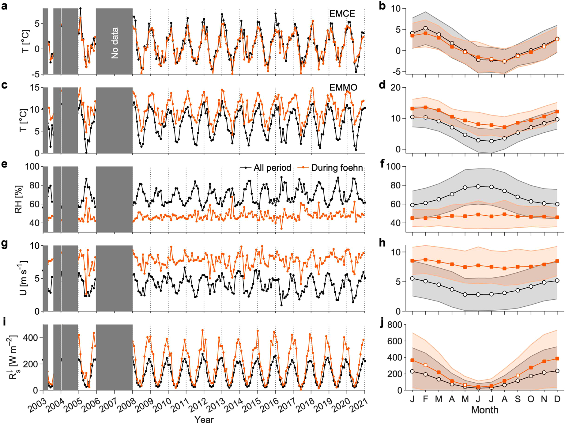
Figure 5 compares the monthly climatology of variables such as air temperature, relative humidity, wind speed, and downward shortwave radiation during foehn events with the entire period. During foehn events, the monthly air temperature at EMMO consistently exceeds that of the entire period by 0.4–10.1°C (Fig. 5c). The temperature difference is particularly high between May and July (Fig. 5d). On the other hand, the air temperature at EMCE shows similar temperature variability during both the foehn events and the entire period (Figs. 5a and b). Monthly relative humidity is consistently lower during foehn events than during the entire period (Fig. 5e). For all seasons, monthly mean relative humidity remains nearly constant, ranging from 45%–50% during foehn events (Fig. 5f). Similar to relative humidity, the monthly mean wind speed during the foehn events is higher than that for the entire period (Fig. 5g). The monthly mean wind speed during foehn shows no clear seasonality, ranging from 7.5 to 8.5 m s−1 and consistently higher than that for the entire period (Fig. 5h). Because the relative humidity increases and wind speed decreases in most of the winter months due to seasonality, the differences are maximised in those periods (Figs. 5f and h). Downward shortwave radiation is higher during the foehn events than it was for the entire period (Fig. 5i). Between November and February, the shortwave radiation is more than 100 W m−2 higher than that during the entire period, with the largest difference of 136 W m−2 was found in December (Fig. 5j). In contrast, the difference is limited to the winter months between May and July.
Monthly (left panels) and monthly climatology (right panels) variables calculated for the entire period (black) and foehn events (orange) for (a,b) air temperature at EMCE, (c,d) air temperature at EMMO, (e,f) relative humidity at EMMO, (g,h) wind speed at EMMO, and (i,j) downward shortwave radiation at EMMO. The filled orange squares indicates that the difference between the two monthly mean variables is statistically significant (p < 0.05) based on the two-sample t-test. T–air temperature, RH–relative humidity, U–wind speed and $R^{\downarrow }_{s}$ –downward shortwave radiation.
It is worth noting that wind speed and downward shortwave radiation were not used to detect foehn winds (Section 2.2). The fact that we observe a higher wind speed and larger downward shortwave radiation during the foehn event increases confidence in the plausibility of the detection criteria. Both increased winds and shortwave radiation fit well with the meteorological conditions during foehn events (e.g., Elvidge and Renfrew, Reference Elvidge and Renfrew2016).
4. Discussion
4.1 Foehn winds influence surface ablation
The foehn events detected are compared with the modelled energy and surface mass balances reported in MM22. Figure 6 shows the daily mean surface ablation, net shortwave radiation, net longwave radiation, sensible heat flux, and latent heat flux vs. mean air temperature for days defined as foehn days or non-foehn days. Temperature dependence is approximately 1.5 times higher for surface ablation on foehn days than for surface ablation on non-foehn days (Fig. 6a). This difference in the surface ablation arises from the enhanced sensible heat flux (Fig. 6d) and net shortwave radiation (Fig. 6b) during foehn days. The sensible heat flux during the foehn days is often higher than the sensible heat flux during non-foehn days because of the higher air temperature and wind speed (Fig. 5). It has been hypothesised that the downward shortwave radiation increases during foehn due to cloudless conditions on the lee side of the Andes (e.g., Temme and others, Reference Temme, Turton, Mölg and Sauter2020). A similar hypothesis has been proposed for ice shelves in the Antarctic Peninsula (Grosvenor and others, Reference Grosvenor, King, Choularton and Lachlan-Cope2014; Elvidge and others, Reference Elvidge2015). Our data supports this hypothesis and indicates that it enhances the surface ablation of the glacier. The downward shortwave radiation sampled during foehn events is higher than the mean insolation for the entire period (Fig. 5i), which is particularly significant in the summer months (Fig. 5j). Foehn events cause more frequent higher net short wave radiation than during non-foehn events (Fig. 6b).
(a) Daily mean surface ablation, a, vs. daily mean temperature, T, for foehn days (orange dots) and non-foehn days (grey dots). The point surface mass and energy balance are calculated at S1 using the meteorological dataset obtained at EMMO (Minowa and others, Reference Minowa, Skvarca and Fujita2022). Orange and grey lines represent the best-fit linear trend. Similar scatter plots for (b) shortwave radiation R s, (c) longwave radiation R l, (d) sensible heat flux H s, and (e) latent heat flux H l. Relative frequency of each variable is indicated by a histogram along the margin of the panel. Orange and grey dots represent the relative frequency of individual variables for foehn and non-foehn days. If the mean value for each bin is statistically significant based on the two-sample t-test, we mark the orange dots with an open orange circle. (f) Scatter plot of air temperature and latent heat flux for foehn days. The marks were coloured by the difference between observed relative humidity, RH, and the threshold relative humidity, RHth.

Latent heat flux shows two different aspects, which dependent on the gradient in humidity (Fig. 6e). We define the threshold of relative humidity to be RHth = e s0/e s × 100, where e s0 and e s are the saturated vapour pressure at 0°C and given air temperature, respectively. The vapour pressure was calculated using the Tetens formulation (Tetens, Reference Tetens1930). Thus, when the observed relative humidity is larger than RHth, condensation will take place, whereas when the relative humidity is less than RHth, we expect evaporation (Fig. 6f). Previous studies highlight the importance of evaporation during foehn winds in terms of energy balance (e.g., Hayashi and others, Reference Hayashi, Hirota, Iwata and Takayabu2005; Shestakova and others, Reference Shestakova, Chechin, Lüpkes, Hartmann and Maturilli2022). Sensible heat flux was nearly cancelled by latent heat flux (Hayashi and others, Reference Hayashi, Hirota, Iwata and Takayabu2005). However, at Glaciar Perito Moreno, foehn winds are not dry enough to allow evaporation/sublimation to take place because of the high air temperature and moisture (Fig. 6e). This is a characteristic meteorological condition found in Patagonia, where the glaciers are located in warm and moist climatic conditions.
Next, we show how foehn winds influence the surface ablation of the glacier by comparing daily foehn hours, energy balance, SMB, and meteorological records in 2011 (Fig. 7). When foehn events are detected, we also observe an increase in sensible heat flux and a decrease in SMB (Figs. 7a–c). One of the largest foehn events and its influence on the SMB is detected in early April 2011 (highlighted by a grey band on Fig. 7a). The daily wind speed and air temperature reaches 11.3 m s−1 and 17.5°C, respectively (Figs. 7d and f). The modelled SMB reaches −0.22 m w.e. d−1, which is the most negative daily value estimated for 2011 (Fig. 7b). This negative SMB may be explained by a large sensible heat flux (Fig. 7c), which reaches 582 W m−2, approximately six times larger than the net shortwave radiation flux (96 W m−2). The latent heat flux is also relatively high during this event (166 W m−2) due to a relatively high humidity compared to the threshold relative humidity (Fig. 7f).
Example of the daily foehn hours, meteorological conditions, energy flux, and surface mass balance in 2011. (a) Time series of daily detected cumulative foehn hours. The horizontal dashed line indicates the 10-h threshold, which defines the foehn day. Daily mean (b) modelled (b m) and observed (b o) point surface mass balance, and (c) the four energy flux components, including net shortwave radiation (R s), net longwave radiation (R l), sensible heat flux (H s), and latent heat flux (H l). Surface and energy balances were calculated at S1 in MM22 (Fig. 1d). The vertical grey bands highlight the timing of one of the greatest foehn events. Daily mean (d) air temperature (T) at EMMO and EMCE, (e) temperature lapse rate calculated between EMMO and EMCE (Γ), and (f) wind speed (U) and relative humidity (RH) at EMMO. On the panel (f), we also show the threshold relative humidity (RHth) for the comparison.

We calculated the contribution to surface ablation during foehn days (Fig. 8). The mean annual surface ablation during foehn events from 2005–2020 is 3.5 m w.e. a−1, or 20% of the annual surface ablation (Fig. 8a). It ranges from 1.8 to 4.6 m w.e. a−1, accounting for 11% to 27% of the annual surface ablation (Fig. 8a). The mean annual surface ablation during foehn events varies between 2.9 m w.e. a−1 and 4.0 m w.e. a−1 by changing the 10-hour criteria ±1 hour. Sensitivity in the detection algorithm is dependent on threshold choice (Section 3.2). Differences in the detected foehn hours led to a standard deviation of the mean annual ablation during foehn events of ±0.5 m w.e. a−1.
(a) Annual surface ablation during foehn (orange bar) and non-foehn days (white bar). The fraction (%) of surface ablation during foehn and non-foehn days is indicated inside individual bars. (b) Monthly surface ablation during foehn (orange bar) and non-foehn days (white bar). The orange and black coloured numbers are the fraction of surface ablation during foehn and non-foehn days, respectively.

On the Antarctic Peninsula, the contribution of foehn wind-induced ablation of the total melt is reported to be 3.1% (Laffin and others, Reference Laffin2021), which is smaller than at Glaciar Perito Moreno. The influence of foehn winds is particularly high (up to 18%) close to the mountain range of the Antarctic Peninsula, where the winds funnel through mountain canyons. Glaciar Perito Moreno is located near the Andean peaks and flows through a valley surrounded by steep mountain terrains (Fig. 1). Foehn winds may be enhanced by funnelling winds through these topographies. The contribution to melting during foehn events also varied seasonally (Fig. 8b). Mean seasonal surface ablation during foehn events is determined to be 0.57 m w.e. month−1 in DJF and 0.36 m w.e. month−1 in SON, whereas the mean ablation is approximately 0.20 m w.e. month−1 in MAM and 0.08 m w.e. month−1 in JJA (Fig. 8b). We find that a relatively large contribution to foehn-induced melting to the total surface melting occurs during JJA (24–31%) and SON (21–26%) more than during DJF (20–23%) and MAM (17–20%). These differences are due to limited surface melting during winter months (Minowa and others, Reference Minowa, Skvarca and Fujita2022) and the frequent occurrence of foehn events during spring (Fig. 2j).
Further qualitative analysis evaluating the processes underlying glacier ablation and its interannual variability is hindered by the daily resolution of the energy and surface mass balance calculation. However, surface mass balance clearly shows a higher ablation rate during foehn days than that during non-foehn days (Fig. 6a). In addition, the interannual variability in the point SMB at S1 is dominated by the variability in the sensible heat flux modulated by air temperature variability, implying the possible influence of foehn winds on surface ablation (Minowa and others, Reference Minowa, Skvarca and Fujita2022). Therefore, we compare the annual foehn frequency (Fig. 3) and mean annual temperature and EMMO and EMCE (Fig. 5i) to infer the influence of foehn winds on surface ablation. Annual foehn frequency and mean annual temperature at EMMO do not show a significant positive relationship (r = 0.34, p < 0.24). On the other hand, a significant negative correlation was found between annual foehn frequency and mean annual temperature at EMCE (r = −0.65, p < 0.01). These relationships imply that foehn winds only weakly relate to the interannual variability of surface ablation at S1. This is because the temperature of the original upwind air mass negatively relates to the frequency of foehn events. It seems that the increased air temperature due to foehn events is compensated by the relatively cold air mass from the west. Further analyses are required to elucidate the underlying mechanisms controlling surface mass balance. Such analysis can be performed by computing the relative contribution of each energy flux component during foehn events and non-foehn events with an hourly resolved energy balance model (e.g., Laffin and others, Reference Laffin2021). It may also be worth measuring meteorological conditions on the glacier to take into account micro-climates caused by interactions at the atmospheric boundary, which we did not investigated in this study. We discuss the importance of the temperature differences between EMMO and EMCE with regard to glacier-wide surface ablation is discussed in Section 4.2. We also discussed the relationship between large-scale climate and temperatures observed at EMCE in Section 4.3.
4.2 Implications for air temperature distribution
Our long-term air temperature records are unique in the region, where in situ and long-term meteorological records are rarely reported (Weidemann and others, Reference Weidemann2018; Bravo and others, Reference Bravo2019; Temme and others, Reference Temme, Turton, Mölg and Sauter2020; Minowa and others, Reference Minowa, Skvarca and Fujita2022). Intriguingly, the temperature at EMMO and EMCE shows different interannual variability (Figs. 3 and 9b,c), which has important implications for spatial distribution of air temperature and we expect influences on local-scale climates, particularly at EMMO. For example, previous SMB modelling studies set the lapse rate to be temporally and spatially constant at 6.5°C km−1 (e.g., Schaefer and others, Reference Schaefer, Machguth, Falvey and Casassa2013, Reference Schaefer, Machguth, Falvey, Casassa and Rignot2015) or to vary monthly (Mernild and others, Reference Mernild, Liston, Hiemstra and Wilson2017). This can introduce uncertainty in derived surface ablation when the lapse rate changes spatiotemporally (Bravo and others, Reference Bravo2019). At Glaciar Perito Moreno, the lapse rate is previously estimated to be 8.0°C km−1 based on field observations (Takeuchi and others, Reference Takeuchi, Naruse and Skvarca1996; Stuefer and others, Reference Stuefer, Rott and Skvarca2007). Takeuchi and others (Reference Takeuchi, Naruse and Skvarca1996) reported that no clear seasonality in lapse rate was detected by their two temperature sensors located in the forest at the coastline, and another 150 m higher on ice. Stuefer and others (Reference Stuefer, Rott and Skvarca2007) also placed a weather station also on the coastline of the lake, and another about 400 m higher on the glacier. Our mean lapse rate of 5.6°C km−1 is lower than previously reported values. It also shows clear seasonal and diurnal variability, with a seasonal maximum from October to November (up to 6.6°C km−1) and a seasonal minimum from May to July (down to 4.5°C km−1) (Figs. 2c and d). The main difference with our observations is that EMCE is located at a much higher elevation of 1260 m, compared to the other stations are located along the coastline (Fig. 1e). Thus, the temperature at EMCE represents the free atmospheric temperature, which causes a difference in the lapse rate reported by previous studies due to local climate, as detailed in the following section. This is supported by our observation that the mean air temperature at EMCE is similar during all foehn periods (Figs. 5a and b).
The monthly anomaly of foehn hours, the temperature at EMMO and EMCE (δT), temperature lapse rate (δΓ) and wind speed δU, and climate indexes. (a) Orange bars and thick orange line indicate the monthly anomaly of the foehn hour and its 3-year running average. (b) Grey bars and thick black lines indicate the monthly air temperature at EMMO and its 3-year running average. A similar plot for (c) air temperature at EMCE, (d) lapse rate, and (e) wind speed. Also indicated are (f) SAM and (g) ENSO indexes with a 3-year running average (thick lines). A large-scale atmospheric circulation pattern is shown in Fig. 10 during the two periods and is indicated by light grey-shaded areas from 2008–2013 and 2015–2016.

Mean wind speed, U (black arrows and coloured contour) and sea level pressure (red contours) during (a) period 1 and (b) 2. Mean anomaly of wind speed, δU, (black arrows and coloured contour) and sea level pressure (red contours) during (c) period 1 and (d) 2. The two periods are indicated in Fig. 9 by light grey shaded areas.

We discuss the large variability of temperature lapse rates resulting in foehn, fog, and katabatic winds. Marked air temperature differences, for example, were observed in 2009 and 2016 (Fig. 3a). In 2009, while the annual temperature at EMMO was close to the mean value, the annual temperature at EMCE shows a negative anomaly primarily due to the negative anomaly in SON (Fig. 3c). The wind speed anomaly shows positive values during SON in 2009 (Fig. 4 in MM22). The highest monthly foehn hours was detected during SON in 2009 (Fig. 2i). These results suggest that the westerlies were strengthened during SON in 2009, resulting in more frequent foehn events at the glacier. With regard to glacier ablation, 2009 shows relatively lower surface ablation over the observed period (Fig. 8a). It is also expected that glacier-wide surface ablation is low for this year because the temperature at EMCE showed the lowest temperature anomaly (Fig. 3a).
In contrast, we observe a positive annual temperature anomaly at EMCE when a marked difference was found in MAM (Figs. 3a and e). The year 2016 is also the year a severe drought hit southern South America (Garreaud, Reference Garreaud2018), causing a large mass loss anomaly on the Patagonian icefields (Gómez and others, Reference Gómez2022). Figure 12 shows the meteorological records for 2016 with daily mean variables. During MAM in 2016, high relative humidity, high downward shortwave radiation, and low wind speed are observed (Fig. 12). These meteorological conditions favour foggy weather because of the interaction of the atmosphere and the lake. The lake surface temperature is several degrees higher than the atmospheric temperature (Minowa and others, Reference Minowa, Sugiyama, Sakakibara and Skvarca2017), which enhances evaporation and causes the formation of fog over the lake. Figure 13 presents an example where the terminus of the glacier is partly covered by fog, whereas sunny conditions exist at high altitudes. Hence, the temperature lapse rate was small in 2016 (Fig. 3a), and the glacier surface was exposed to a higher air temperature than in other years.
Intriguingly, between 3–5 February 2019, saw unprecedented high temperatures due to a heatwave were observed over Patagonia (e.g., Jacques-Coper and others, Reference Jacques-Coper, Veloso-Aguila, Segura and Valencia2021). It has been demonstrated that these heat waves are induced by warm air advection and enhanced radiative heating caused by anticyclonic anomalies over the southwest Atlantic Ocean (Jacques-Coper and others, Reference Jacques-Coper, Brönnimann, Martius, Vera and Cerne2016, Reference Jacques-Coper, Veloso-Aguila, Segura and Valencia2021). High temperatures are also observed at our AWSs (Fig. 14). The temperatures recorded at EMCE reached 24.8°C at 16:00 on 4 February 2019, while the air temperature at EMMO was 15.4°C at that time (Fig. 14a). Wind speed was also relatively low ~5 m s−1 (Fig. 14e). Due to the relatively low air temperature and wind speed, the sensible heat flux was limited, resulting in a small surface mass balance (Figs. 14f and g). A much larger negative surface mass balance was indeed observed during the foehn event that occurred on February 15th due to warm temperatures and high wind speeds (Figs. 14a, e, and f). We interpret the negative temperature inversion during the heatwave as a result of the influence of katabatic winds (Oerlemans and Grisogono, Reference Oerlemans and Grisogono2002). The warm ambient air mass cooled due to the interaction between the atmosphere and glacier surface during ice melting and flowing down the glacier.
Overall, the lapse rate varied spatially and temporally due to the local-scale meteorology described above. Distributing air temperature with a fixed lapse rate misses these aspects and introduces biases in the calculated surface mass balance. On the other hand, our long-term meteorological records are obtained on the bedrock beside the glacier, which means that micro-scale processes are not observed. Air mass temperature on the glacier near the atmospheric boundary between glacier surface and free-atmosphere vary drastically due to micro-scale meteorological conditions and therefore the temperature lapse rate (e.g., Gardner and others, Reference Gardner2009). Further study is beneficial for exploring the relationships between local-scale and micro-scale climates, as well as to conduct a glacier-wide surface mass balance calculation. This calculation has been validated with the help of our stake network (Fig. 1d).
4.3 Large-scale climate influences on foehn
The meteorological records and occurrence of foehn vary interannually over the study period (Figs. 2 and 3). We compared foehn occurrence with SAM and ENSO and investigate their potential connection. In MM22, they compared air temperature and wind speed at EMMO with SAM and ENSO, showing a potential connection between them. Positive SAM and La Niña conditions favour high air temperature and wind speed, whereas negative SAM and El Niño favour low temperature and wind speed. Thus, the surface mass balance can be modulated by these large-scale climates. In this study, we also compare the air temperature at EMCE and the lapse rate between EMCE and EMMO with these climate indices (Fig. 9). Upon comparison, seasonal variability is removed from the meteorological records by subtracting the monthly mean climatology (2003–2020). Correlation coefficients among variables are listed in Table 1.
Correlation coefficients between the temperature at EMCE, lapse rate, ENSO, and SAM. In the first row, the monthly temperature and lapse rate are compared with the monthly SAM and ENSO. In the following rows, the seasonal mean temperature and lapse rate are compared with the seasonally averaged SAM and ENSO. The significance level of the correlation p-values of 0.1 and 0.05 are bolded and underlined. Seasonal variability is removed upon comparison with meteorological records by subtracting the mean monthly value over the period 2003–2020

No simple relationship was found between foehn occurrence and these climate indices (Table 1). A weak negative correlation was found in MAM between foehn occurrence and ENSO (Table 1). Stronger relationships were found in ENSO with the temperature at EMCE (r = 0.69, p < 0.01) and with the lapse rate (r = −0.76, p < 0.01). To understand how foehn occurrence is controlled by large-scale climate circulation, the mean and mean anomaly of wind speed and sea level pressure is calculated during two periods when stronger ENSO and SAM are observed. Positive SAM and La Niña are observed most of the time during Period 1 from 2008–2013, with stronger positive SAM and El Niño during Period 2 from 2015–June 2016 (Fig. 9). For both periods, the mean and mean anomaly atmospheric fields show a pressure change over the Amundsen Sea Low (Fig. 10). During Period 1, the strengthening of the Amundsen Sea Low over the Drake passage can also be observed, resulting in an enhancement of the westerly winds in the study region (Figs. 10a and c). In contrast, during Period 2, the weakening of low-pressure caused a reduction and southward shift of the westerlies in the study region (Figs. 10b and d).
Several studies have suggested that SAM and ENSO influence variations in the Amundsen Sea Low (Fogt and others, Reference Fogt, Bromwich and Hines2011; Turner and others, Reference Turner, Phillips, Hosking, Marshall and Orr2013; Hosking and others, Reference Hosking, Orr, Marshall, Turner and Phillips2013; Vera and Osman, Reference Vera and Osman2018; Fogt and Connolly, Reference Fogt and Connolly2021; Carrasco-Escaff and others, Reference Carrasco-Escaff, Rojas, Garreaud, Bozkurt and Schaefer2023). The SAM, defined by the normalised monthly mean sea-level pressure difference between mid-latitude (40°S) and high-latitude (65°S), substantially modulates the Amundsen Sea Low. During positive SAM, the westerly winds intensify and shift towards Antarctica (Thompson and Wallace, Reference Thompson and Wallace2000), which amplifies local meridional wind anomalies, and the Amundsen Sea Low tends to be stronger than during normal conditions (Turner and others, Reference Turner, Phillips, Hosking, Marshall and Orr2013). In contrast, the La Niña phase in ENSO enhances and broadens the Amundsen Sea Low (Turner and others, Reference Turner, Phillips, Hosking, Marshall and Orr2013). The wind speed and sea-level pressure anomalies during Period 1 are consistent with previous reports (Fig. 10c), resulting in an enhancement of the westerly winds and foehn occurrence (Fig. 9).
Wang and Cai (Reference Wang and Cai2013) report that ENSO and SAM are not independent. El Niño events tend to occur with a negative SAM, while La Niña events occur with a positive SAM. Thus, the strong positive SAM associated with El Niño event observed between 2015 and 2016 (Period 2) remains an unsolved question (Vera and Osman, Reference Vera and Osman2018). These unprecedented climate anomalies caused severe drought in southern Patagonia in 2016 (Garreaud, Reference Garreaud2018). In addition to this finding, our local weather station datasets indicate a substantial decrease in wind speed at EMMO and temperature warming at EMCE (Figs. 9e and c, respectively), resulting in a decrease in foehn occurrence (Fig. 9a), which continued even after the climate anomalies of mid-2016 were over (Fig. 9). The mean wind speed and sea-level pressure anomalies indicate a weakening of the Amundsen Sea Low and therefore a reduction in westerlies during Period 2 (Fig. 10b). This extreme climate anomaly caused a reduction in foehn events, and surface ablation is relatively reduced between 2015 and 2017 (Fig. 8a).
Further investigation of these and other periods is necessary to better understand the influence of climate anomalies on glaciers’ surface mass balance. Westerlies have migrated polarward over the last few decades, as indicated by the positive SAM trend (e.g., Gillett and others, Reference Gillett, Kell and Jones2006; Swart and Fyfe, Reference Swart and Fyfe2012), and this trend is projected to continue in this century (Goyal and others, Reference Goyal, Sen Gupta, Jucker and England2021). Additionally, stratospheric ozone depletion and increased greenhouse gas concentration favour stronger El Niño in the future (e.g., Gillett and others, Reference Gillett, Kell and Jones2006; Arblaster and Meehl, Reference Arblaster and Meehl2006; Cai and others, Reference Cai2018). Because changes in large-scale climate influence the variability of the westerlies (Fig. 10), they also control the variability of foehn occurrence (Fig. 9). Because the ongoing variations in westerly winds due to anthropogenic forcing alter the dominant process of surface mass balance in Patagonian glaciers, the continuation of meteorological field observations is invaluable for understanding glacier behaviour in Patagonia.
5. Conclusions
An algorithm is applied to detect foehn events based on hourly meteorological records observed at Glaciar Perito Moreno in the southern Patagonian icefield from 2003–2020. We detected 15 438 hours of foehn, or an average of 89 hours per month and 1073 hours per year on average. The number of foehn hours is approximately three times larger from October to January (austral spring and summer) than between May and July (austral winter). Enhanced wind speed during summer from the southern Pacific Ocean resulted in a higher occurrence of foehn on the lee side of the Andes. Surface ablation during foehn hours accounts for 20% of annual surface ablation. The surface ablation rate increased significantly during foehn events due to the increased sensible heat flux and net shortwave radiation. However, foehn occurrence was only weakly related to the temperature at the lower EMMO station, and negatively related to the temperature at the upper EMCE station. This suggests that foehn winds are not the only meteorological condition that determines strong surface ablation and its interannual variability in Patagonia.
The temperature observed at EMCE at ~1260 m a.s.l. and EMMO at 192 m a.s.l. shows different variability due to temperature inversion because of the influence of local-scale weather conditions, i.e., foehn, fog, and katabatic winds. Calm sunny days in winter cause a large temperature difference between the atmosphere and the lake. The fog, which partly covers the glacier terminus, forms over Lago Argentino, causing a temperature inversion. On the other hand, on warm but calm sunny days in summer, the ambient warm air interacts with the glacier surface and cool air flows down the glacier. This temperature inversion as a result of the local climate may play an important role in determining the glacier-wide surface mass balance.
No simple relationship was found between foehn occurrence and large-scale climate variability. However, foehn occurrence appears to be related to the strength of the westerlies, which are related to the location and development of the Amundsen Sea Low under the influence of SAM and ENSO variability. For example, a reduction of foehn occurrences occurred between 2015 and 2017, coinciding with strong El Niño and positive Southern Annular Mode by weakening the westerlies. Considering that these large-scale conditions are anticipated to continue in the coming decades, the future evolution of foehn events and their relationship with projected changes to ENSO and SAM would be an important area of future research. Because our observations and analyses are limited to the period from 2003–2020, continuing observations in the region is invaluable for understanding the fluctuation of glaciers, which are losing ice mass at the fastest rate in the world.
Data
Meteorological data used in the study are available upon reasonable request to PS. ERA5 reanalysis dataset is available at https://cds.climate.copernicus.eu/. SAM and ENSO indices are available at https://climatedataguide.ucar.edu/climate-data/marshall-southern-annular-mode-sam-index-station-based/ and https://psl.noaa.gov/enso/mei/, respectively.
Acknowledgements
We are grateful to all those who helped in the field campaigns, in particular to Carlos Domínguez for collecting the climate data. Hielo y Aventura provided invaluable logistical support at the glacier. The manuscript was improved by comments and suggestions from Charlie Zender, an anonymous reviewer, Chief Editor Hester Jiskoot and Scientific Editor Carleen Reijmer. The English text was corrected by Fluent Prose. MM was supported by Grant-in-Aid for JSPS Fellows (JP20J00526) and JSPS KAKENHI Grant (JP22K14093). Datasets were analysed using Matlab R2018a. Figures were produced using Matlab R2018a and QGIS 3.20.
Author's contributions
MM led the study with support from KF and PS. PS initiated and managed the meteorological and surface ablation observations. MM contributed to field observation and instrument maintenance. KF developed and contributed to the surface mass balance calculation. All authors contributed to the discussion of the results.
Appendix 1: Additional Figures
(a) Cumulative distribution frequency of foehn hours using the algorithm. (b) Mean daily surface ablation calculated during foehn (orange triangle) and during non-foehn events (grey square) at S1. Total surface ablation dependent on foehn hours is indicated by green circles. The shaded areas indicate one standard deviation of surface ablation. The vertical dashed line indicates the 10-hour criteria to define a foehn day. (c) The sum of possible overestimation and underestimation is calculated with different threshold hours. The 10-hour criteria minimise the error that arose from the choice of threshold.

Daily meteorological records from 2016 are indicated by red lines. (a) Air temperature (T) at EMCE and (b) EMMO, (c) temperature lapse rate (Γ), (d) relative humidity (RH), (e) downward shortwave radiation ($R^{\downarrow }_{s}$ ), (f) wind speed (U), and (g) wind direction (U d). The background grey lines and shaded areas indicate the mean daily value and its one standard deviation calculated from 1996–2020.

(a) Satellite image captured on 16 May 2016 by Landsat 7. Low cloud cover over Lago Argentino. (b) A cloud-free satellite image captured on 3 March 2021 by Sentinel 2. The two AWSs are indicated by red triangle and circle. Note that the black stripes on the panel (a) are due to a failure of the Landsat 7 scan line corrector.

Hourly meteorological, surface mass balance, and energy balance records between 1–17 February 2019. (a) Air temperature (T) at EMMO and EMCE. (b) Temperature lapse rate (Γ). (c) Relative humidity (RH). (d) Downward shortwave radiation ($R^{\downarrow }_s$ ). (e) Wind speed (U). (f) Observed (b o) and modelled (b m) point surface mass balance at S1. (g) Component of energy flux for ice melting: R s—net shortwave radiation, R l—net longwave radiation, H s—sensible heat flux and H l—latent heat flux. The surface energy balance components are after MM22. Vertical orange areas indicate detected foehn hours, whereas grey areas highlight the temperature inversion observed during the heatwave between 3–5 February.


 Open access