


Introduction
Over the last several decades, the resolution and availability of synthetic aperture radar (SAR) data have increased dramatically (Ignatenko and others, Reference Ignatenko2020), creating new potential opportunities at the intersection of glaciology and remote sensing (e.g., Yang and others, Reference Yang, Li, Huang, Tian and Chen2016). SAR, which was first applied as a glaciological tool in 1993 to measure the velocities and grounding line positions of Antarctic ice streams (Goldstein and others, Reference Goldstein, Engelhardt, Kamb and Frolich1993), allows for remote sensing of glacier motion regardless of daylight or weather conditions (Joughin and others, Reference Joughin, Smith and Abdalati2011). Furthermore, as a radar is phase sensitive, interferometric SAR (InSAR) techniques can be applied to resolve glacier motion at the centimeter scale, regardless of the spatial resolution (essentially the pixel size) of the sensor (e.g., Goldstein and others, Reference Goldstein, Engelhardt, Kamb and Frolich1993; Gray and others, Reference Gray1998). Due to its accuracy, InSAR has been used to measure and investigate ‘mesoscale’ glacier phenomena that result in subtle (i.e., centimeter-scale) perturbations in surface ice velocity fields, such as migration of subglacial water pockets (Fatland and Lingle, Reference Fatland and Lingle2002) or movement of ice-shelf grounding lines (Rignot, Reference Rignot1998; Rabus and Lang, Reference Rabus and Lang2002).
However, while InSAR delivers high-resolution deformation measurements, it is only sensitive to motion in the line-of-sight (LOS) direction of the radar and is plagued by a number of complex pitfalls stemming from the cyclical nature of phase data (Yu and others, Reference Yu, Lan, Yuan, Xu and Lee2019). Thus, Gray and others (Reference Gray1998) introduced a second SAR-based technique known as speckle tracking that avoids many of the InSAR pitfalls while also measuring motion along both axes of the SAR image. However, unlike InSAR, the accuracy of SAR speckle tracking is linked to the pixel size of the image (Gray and others, Reference Gray, Short, Mattar and Jezek2001; Bamler and others, Reference Bamler, Eineder, Adam, Zhu and Gernhardt2009) and early SAR sensors suffered from coarse spatial resolutions, with pixel sizes on the order of 10 m or larger. Thus, for a number of years, researchers were often forced to choose between InSAR, which was directionally limited and complex, or the simpler and more versatile, but much lower resolution, speckle tracking.
The spatial resolution of SAR sensors has increased significantly since the early 1990s, particularly through introduction of sub-meter-resolution spotlight modes, which now allow SAR speckle tracking to approach the resolution of (regular, stripmap mode) InSAR. However, high-resolution SAR speckle tracking, which is able to resolve mesoscale glacier motion, remains a relatively under-exploited tool, generally only being used to measure glacier- or ice-sheet-wide velocity fields, albeit at higher resolutions.
Spatially discontinuous glacier motion, which is poorly understood, in part due to a lack of observational evidence, is one form of glacier motion that can now be measured using high-resolution speckle tracking. Discontinuous glacier motion generally results from the brittle failure and fracture of ice and can lead to glacier velocity fields that are spatially or temporally discontinuous (e.g., serac fall or glacier collapse). Discontinuous glacier motion also results in a variety of glacier structures such as crevasses and seracs and can significantly contribute to glacier dynamics (Faillettaz and others, Reference Faillettaz, Funk and Vincent2015; Colgan and others, Reference Colgan2016).
Speckle tracking
Single look complex (SLC) images, essentially SAR images with minimal processing applied post-focusing, exhibit a characteristic speckle pattern. This speckle pattern is controlled by the roughness of the glacier surface at the sub-pixel scale and can be tracked between SLCs, provided that the glacier surface remains relatively unchanged (i.e., has non-zero interferometric coherence), as the speckle pattern is advected down-glacier (Joughin, Reference Joughin2002; Moreira and others, Reference Moreira2013). Speckle tracking itself is done by selecting a multi-pixel chip of fixed shape from an initial SAR image and searching for a matching chip in a subsequent image using the normalized two-dimensional (2-D) cross-correlation coefficient (NCC) as a similarity measure. The NCC is generally calculated using the normalized product of SAR image intensities, but in some cases, the interferometric phase is included and this then makes the similarity measure to be optimized equal to the (intensity weighted) interferometric coherence (Michel and Rignot, Reference Michel and Rignot1999; Gray and others, Reference Gray, Short, Mattar and Jezek2001; Joughin, Reference Joughin2002). In theory, for featureless areas, phase-based SAR speckle tracking is more accurate than its intensity-based counterpart, but is more computationally expensive and requires accounting for systemic phase differences due to factors such as topography (Bamler and Eineder, Reference Bamler and Eineder2005; De Zan, Reference De Zan2014). Thus, in real-world scenarios, phase-based speckle tracking is used less frequently and may not outperform intensity speckle tracking. It is important to note, however, that phase-based speckle tracking and intensity speckle tracking are fundamentally linked, as a variation in coherence (i.e., decreases in complex cross-correlation due to changing radar scatterers) will lead to corresponding differences of the speckle pattern between chips as the spatial signature of the pattern is ultimately controlled by the phase and amplitude response of the radar scatterers within the resolution cell.
A major benefit of SAR speckle tracking is that it is able to unambiguously resolve glacier motion and benefits greatly from high-resolution SAR images as its accuracy is directly linked to pixel size. Moreover, the coherence (i.e., similarity resulting from an unchanged ground/glacier surface) of a scene pair is often better preserved with high-resolution SAR images (e.g., Mohammadimanesh and others, Reference Mohammadimanesh, Salehi, Mahdianpari, Brisco and Motagh2018) as smaller pixels are less likely to capture an altered radar scatterer (Closson and Milisavljevic, Reference Closson and Milisavljevic2017). Thus, high-resolution speckle tracking presents a powerful, but underleveraged, tool for investigating ice dynamics associated with meso-glacier motion. In this study, we develop an intensity prefilter for SLCs designed to improve the performance of high-resolution SAR speckle tracking and use this improved method, in conjunction with a 2-D cross-sectional ice-flow model, to investigate unusual hypothesized mesoscale discontinuous glacier motion on Thompson Glacier, Canadian High Arctic. Potential evidence of this motion comes from preliminary InSAR analysis of the area that shows broken interferometric fringes, a phenomenon that has previously been attributed to discontinuous motion (e.g., Rignot, Reference Rignot1996; Kobayashi and others, Reference Kobayashi, Morishita and Yarai2018; Millan and others, Reference Millan2022a), albeit at much larger spatial scales.
Study site
The focus of this study, Thompson Glacier, is located at the head of Expedition Fjord on Umingmat Nunaat (Axel Heiberg Island) in the Canadian Arctic Archipelago (Fig. 1). Thompson Glacier, the largest of the Expedition Fjord glaciers, is an outlet glacier of Mueller Ice Cap (Müller, Reference Müller1962) and has several named tributary glaciers including Piper (formerly Wreck) Glacier and Astro Glacier. While relatively few glaciological studies have been conducted on Thompson Glacier, the neighboring White Glacier, which is substantially smaller, is one of the most intensively studied (e.g., Hambrey and Müller, Reference Hambrey and Müller1978; Blatter, Reference Blatter1987; Cogley and others, Reference Cogley, Adams, Ecclestone, Jung-Rothenhäusler and Ommanney1996; Thomson and others, Reference Thomson, Zemp, Copland, Cogley and Ecclestone2017) glaciers in the Canadian Arctic largely due to its proximity to the McGill Arctic Research Station (Thomson and Copland, Reference Thomson and Copland2017). Mapping of the Expedition Fjord glaciers shows that, between 1948 and 1995, Thompson Glacier advanced ~950 m while White Glacier retreated 250 m. The reason for this difference remains unclear, but researchers speculate that differing response times to climatic forcings due to size differences or a slow surge on Thompson Glacier may be responsible (Cogley and others, Reference Cogley, Adams and Ecclestone2011).
Expedition Fjord glaciers on Umingmat Nunaat (Axel Heiberg Island), including Thompson Glacier, the subject of this study. The red box indicates the footprint used in developing the intensity rescaling scheme. The arrows indicate, from top to bottom, the Upper Channel, West Channel and Astro Channel across which discontinuous glacier motion is suspected to occur. Coordinates are given in UTM, Zone 15 N. The inset at top right shows the Astro Channel in 2022 near the Piper–Thompson Confluence. The photographer estimates the channel is ~10 m deep and 3 m wide. Astro Channel imagery courtesy of Laura Thomson and satellite imagery courtesy of Esri World Imagery (Esri, 2022).

A key feature of interest in this study is the large supraglacial channel on Thompson Glacier, which we henceforth refer to as the Astro Channel, originating from Astro Lake and extending ~5 km down glacier. Preliminary remote sensing results indicate that discontinuous glacier motion may be occurring around the Astro Channel, although the exact nature and cause of this hypothesized discontinuous motion is unclear. A variety of observations over the last 75 years, beginning with aerial photography in 1948 (photograph 60LT-72PL-C-8M219-72RS-11 AUG. 48-14C, National Archives of Canada), indicate that the channel is a persistent feature. During fieldwork conducted in the spring of 1961, Maag (Reference Maag1963) observed the Astro Channel, noting that it drained Astro Lake and had depths of up to 30 m in some areas. Researchers visiting the Astro Lake area in 1976 and 2008 photographed the Astro Channel, noting that the channel bridges over due to plastic deformation (swisseduc.ch/glaciers). Additionally, satellite imagery dating back to at least 2009 consistently shows the Astro Channel, although the degree to which it is bridged over varies.
Remote sensing methods and data
SAR data
We use SAR speckle tracking to measure the surface velocities of the Expedition Fjord area glaciers with a specific emphasis on the location near the Piper–Thompson confluence. SAR data used in this study (see Table S1 and Fig. S1) are collected with the spotlight beam mode of RADARSAT-2, a Canadian Space Agency SAR satellite with a 24 d repeat orbit, that operates at C-band (5.6 cm wavelength) (Morena and others, Reference Morena, James and Beck2004; Van Wychen and others, Reference Van Wychen2018). These SAR images have pixel sizes of 1.330–1.332 m in range and 0.379–0.414 m in azimuth. The spotlight beam mode itself employs electronic beam steering to dwell on the area of interest for a longer duration than would otherwise occur, resulting in the high image resolution in the satellite flight (i.e., azimuth) direction as compared to other imaging modes (MDA, 2018). The SAR data used in this study are only collected during the winter and spring as low temperatures and low snow accumulation help maintain glacier surface coherence, a prerequisite for accurate InSAR and SAR speckle tracking.
False matches due to high-intensity pixels
Glacier speckle tracking results often contain rectilinear artifacts (see Fig. 2) – a geometry that suggest they are non-physical – due to the speckle tracking algorithm ‘locking-on’ to various features. Here, we investigate the underlying cause of these rectilinear artifacts and develop a compensating method to improve the accuracy of speckle tracking.
Hillshaded (30 × vertical exaggeration) SAR speckle tracking results (for range direction only) from SLCs collected on 5 January 2022 and 29 January 2022 over Thompson Glacier showing rectilinear ‘lock-on’ artifacts. The arrows indicate several of the most obvious artifacts. As expected, the dimensions of these artifacts closely match the speckle tracking chip size, in this case 64 × 192 pixels in range and azimuth respectively (see section on ‘Speckle tracking methods’).

At its core, speckle tracking identifies similar areas in two consecutive SAR images using the NCC, which can be written as

where f(x, y) and g(x, y) are the intensity values of the chips being compared, (x 0, y 0) represents the coordinate translation between images, $\bar {t}$ is the mean intensity of the selected chip and $\bar {f}_{x_0, y_0}$
 is the mean value of the region in f(x, y) that is being searched (Yoo and Han, Reference Yoo and Han2009). Equation (1) involves element-wise multiplication of the demeaned intensities of the two pixels in the same in-chip position. This makes the NCC particularly sensitive to situations in which high intensity pixels are in the same in-chip position, an issue that is compounded by the strong right-skew of a Rayleigh intensity distribution characteristic of an SAR image.
To reduce the prevalence of false matches caused by multiplication of high-intensity pixels, we propose a non-linear intensity rescaling that will be applied to SAR images before speckle tracking to reduce the impact of high intensity pixels on the NCC.
Creating a simulated SAR image pair
To confirm that intensity rescaling can improve SAR speckle tracking performance, and to identify a rescaling that performs well, we develop an SAR simulator capable of producing a realistic glacier speckle tracking pair with a known motion field. We identify three key requirements for a realistic SLC pair: (1) a partially correlated speckle pattern, (2) a glaciologically realistic motion field and (3) realistic terrain (e.g., supraglacial streams, moraines, etc.) and speckle patterns. To generate a realistic SLC pair, we start with a real SAR image, covering a glacierized area, as the initial scene in the speckle tracking pair. For the second image, we use an SLC formed from a combination of speckle patterns, terrain maps and motion fields extracted from actual SAR images of the same glacierized area (see Fig. 3).
Schematic outlining the process for generating the second synthetic SAR image used in the simulated SAR speckle tracking pair. Actual SLC 1 and synthetic SLC 2 will be used as the image pair.

The process begins by selecting an area of interest (see Fig. 1) on Thompson Glacier that contains both the glacier margin, meaning that a significant velocity gradient will be captured, along with a large and perennial supraglacial channel across which discontinuous glacier motion is suspected to occur. Both the glacier margin and the channel provide clusters of high intensity pixels that may result in false speckle tracking matches.
After selecting the area of interest, two (globally coregistered) SLCs are cropped to contain this common area. The two images are chosen to maximize the temporal separation, and thus glacier surface change, which results in the speckle patterns between them being as decorrelated as possible. The selected images were acquired on 15 February 2018 and 22 May 2018, comprising the first and last SLCs available with matching acquisition parameters. The SLC collected on 15 February 2018 will serve as the initial image in the simulated speckle tracking scene pair.
A Lee sigma filter (Lee, Reference Lee1983) with a 3 × 3 pixel window is used to obtain both the terrain backscatter map, T (i.e., a speckle-free image) and the speckle pattern S 1 from the initial real SLC. This filter, chosen for its ease of implementation and low-computational cost, is designed to suppress radar speckle while preserving edges and fine details. A 3 × 3 pixel window is chosen in order to minimize blurring of surface features in the terrain map. The same Lee sigma filter is also used to obtain S 2, the speckle pattern from the second real SLC. The major benefit of obtaining these speckle patterns from real data is that glacier features such as marginal moraines will be captured in S 1 and S 2 if these features happen to exhibit some control on the speckle patterns.
To form the second, simulated SLC in the speckle tracking pair, a speckle pattern that is partially correlated with S 1 is necessary. This partial correlation simulates the minor changes in the glacier surface that are inevitable over the 24 d repeat period of RADARSAT-2. S 3, the speckle pattern for the second simulated SLC, is formed by combining S 1 and S 2 using the Kaiser–Dickman algorithm (Kaiser and Dickman, Reference Kaiser and Dickman1962):

where ρ is the desired coherence. For our experiments, we chose ρ = 0.8, which results in a mean NCC of 0.543 for the simulated scene pair. This value is comparable to the mean NCC, for the same geographic area, of the most coherent scene pairs used in this study and represents a realistic but favorable scenario (i.e., little glacier surface change). To obtain the second SLC for the speckle tracking pair, S 3 is normalized to unit mean to ensure it does not change the overall intensity of the second synthetic SLC and is then multiplied element-wise by the terrain backscatter intensity map T (Xie and others, Reference Xie, Pierce and Ulaby2002).
A realistic glacier motion field is then introduced to the second simulated SLC using Lanczos resampling and a user-defined lookup table. The realistic glacier motion field itself is generated by taking the speckle tracking results from the 15 February 2018 and 11 March 2018 SLCs and smoothing the resulting motion field using a 20 × 60 pixel (~30 m × 30 m) boxcar filter.
Optimal intensity transformation
We begin by using the SAR simulator described above to test intensity transformations that follow

where I represents the normalized intensities, achieved by dividing the original image by the mean intensity of the SLC. The range and step size of k is chosen to ensure that a minimum is captured and that there is a reasonable (~10%) difference in mean absolute error (MAE) between successive steps. k = 1.5 gives the best-performing intensity transformation on the basis of MAE between the speckle tracking results and the imposed motion field. However, despite the measured MAE improvement, the speckle tracking results still pronounce outlier-type errors, appearing as rectilinear artifacts (e.g., Fig. 2), around the bright pixels that form the supraglacial channel in the simulated image pair. Thus, we test a piecewise transformation that applies a higher value of k, denoted k h, to pixels above some intensity threshold. The piecewise transformation is given by

where t is a threshold intensity and the term $( t^{1/1.5}-t^{1/k_{\rm h}})$ ensures that the piecewise function is continuous and monotonically increasing. A grid search with k h ∈ {2, 3, 4, 5} and t ∈ {1, 1.5, 2, 2.5, 3} shows that k h = 3, t = 2 yields the best performance with an MAE of 0.0477. This transformation represents a 23% improvement over the untransformed case for the simulated speckle tracking pair.
Speckle tracking methods
To measure glacier motion, intensity-transformed speckle tracking is performed at the full image resolution (i.e., a one pixel step in both range and azimuth) using an upsampling factor of two and a 64 × 192 pixel correlation chip (prior to upsampling) in range and azimuth respectively. The chip size, which corresponds to a ground footprint of ~80 m × 80 m, is intended to be small enough to capture the glacier motion of interest while still being large enough to provide robust matches. The upsampling factor is chosen as a compromise between accuracy and computational cost (Magnard and others, Reference Magnard, Werner and Wegmuller2017). A minimum cross-correlation threshold of 0.1 is used, where matches that fall below this threshold are discarded. The speckle tracking itself is carried out using the GAMMA software's offset_pwr_tracking function.
Speckle tracking is only capable of measuring the glacier motion field in a 2-D plane defined by the range and azimuth directions. To convert the measurements in this plane into glacier motion, we use the surface-parallel flow assumption (e.g., Cumming and Zhang, Reference Cumming and Zhang1999; Joughin and others, Reference Joughin, Smith and Howat2018) which assumes that the true motion vector lies in the plane that is locally tangent to the glacier surface, equivalent to assuming that emergence/submergence velocities are negligible over the temporal baseline of the speckle tracking pair. In select cases, two speckle tracking results from substantially different look geometries overlap in time and space, allowing for inversion of the full three-dimensional (3-D) velocity field (e.g., Nagler and others, Reference Nagler2012; Wang and others, Reference Wang2019). ArcticDEM 7 (Porter and others, Reference Porter2018) is used to define the locally tangent glacier surface necessary for the surface-parallel assumption and for the geocoding used to align the two speckle results employed in the 3-D velocity inversion.
For scenes of interest that contain the Astro Channel, where speckle tracking results indicate a substantial cross-channel velocity discontinuity, an additional masked speckle tracking is carried out. Here, ice on each side of the channel is tracked separately (i.e., the other side is masked out) to ensure that speckle tracking chips do not straddle the channel itself.
Remote sensing results and discussion
Intensity transformed speckle tracking is used to track glacier motion for the 30 scene pairs (see Table S1) collected over the Expedition Fjord area. In all cases, the scene pairs are formed from SLCs collected 24 d apart. Glacier speeds resulting from speckle tracking under the surface-parallel flow assumption (Fig. 4) match velocity data from NASA ITS_LIVE (Gardner and others, Reference Gardner2018, Reference Gardner, Fahnestock and Scambos2022) closely, with an MAE of 0.52 cm d−1. Note that this comparison masks out ITS_LIVE velocities of <4 cm d−1, as the underlying algorithm is known to perform poorly in areas of slow-moving ice (Lei and others, Reference Lei, Gardner and Agram2021; Williams and others, Reference Williams, Gourmelen and Nienow2021).
Surface flow speed from SAR speckle tracking versus NASA ITS_LIVE data. (a) Average glacier speed as measured by speckle tracking under the surface parallel flow assumption and (b) difference (ITS_LIVE-SAR) between NASA ITS_LIVE data and speckle tracking results. Note that the ITS_LIVE data are annual velocities whereas the speckle tracking data cover only winter and spring. ITS_LIVE velocity data are generated using auto-RIFT (Gardner and others, Reference Gardner2018) and provided by the NASA MEaSUREs ITS_LIVE project (Gardner and others, Reference Gardner, Fahnestock and Scambos2022). Optical imagery courtesy of Esri World Imagery (Esri, 2022).

Broken fringes
The glacier motion maps produced by SAR speckle tracking, along with ArcticDEM (Porter and others, Reference Porter2018), are also used for InSAR analysis. We create interferograms sensitive only to glacier motion along the satellite LOS which show broken fringes in three different areas of Thompson Glacier. In all three cases, the broken fringes align with large, persistent supraglacial channels that are visible in optical satellite imagery dating back until at least 2009 and appearing in the same location in all RADARSAT-2 scenes used in this study which date from 2012, 2013, 2014, 2015, 2018 and 2022. Each channel appears to be fed by an ice-marginal lake. We refer to these three channels as the Upper Channel, West Channel and Astro Channel (see Fig. 1).
Broken InSAR fringes can be the result of (1) discontinuous motion, (2) a topographic discontinuity (i.e., a cliff or other steep topographic feature) that is not present in the DEM or (3) a topographic discontinuity present in the DEM but that did not exist when the SAR data were collected. Mechanism 3 is easily ruled out by examining the DEM, which contains no steep gradients in the areas of the broken fringes. Mechanism 2 can be investigated as fringe spacing resulting from topography would exhibit an inversely proportional stereo-like sensitivity to the spatial baseline (i.e., a measurement of the distance between the two acquisition positions of the SAR satellite) of the scene pairs while fringes from motion fields would remain constant as the spatial baseline changes (Pepe and Calò, Reference Pepe and Calò2017). Examination of consecutive interferograms with the same acquisition parameters (e.g., Figs 5, S2, S3), with baselines that vary by up to a factor of 4, show highly consistent fringe patterns, indicating that the broken fringes result from persistent discontinuous glacier motion.
Broken SAR interferometric fringes across the Astro Channel along with optical imagery. The interferogram in (a) and (c) is created using data from 15 February 2018 and 11 March 2018. The interferogram in (d) is created using data from 11 March 2018 and 4 April 2018. Panels c and d show a close-up of the respective interferogram in the area around the channel. Note that despite the significant difference in B ⊥, the magnitude of the fringe discontinuities is approximately equal in both interferograms, indicating discontinuous motion as opposed to discontinuous topography. Optical imagery courtesy of Esri World Imagery (Esri, 2022).

It should be noted that a spatial discontinuity in the liquid water content of the snowpack may plausibly cause broken interferometric fringes (Minchew and others, Reference Minchew, Simons, Hensley, Björnsson and Pálsson2015). However, the extreme cold and thin Arctic snowpack concurrent with many of the observed broken fringes preclude the presence of liquid water in the snowpack. For example, from 15 February 2018 to 11 March 2018 (see Fig. 5), the maximum temperature recorded at Eureka, the closest weather station located 120 km east of the study site at 100 m a.s.l., never exceeded −18.9°C. Moreover, the aforementioned timeframe is not a special case as we almost exclusively use SAR data collected during winter and early spring (i.e., low-temperature periods) to avoid loss of surface coherence due to melt.
3-D velocity profiles
To characterize and visualize the Astro Channel discontinuity, we plot velocity profiles by sampling 3-D velocity rasters across transects that run perpendicular to the channel. For each profile, velocities are plotted from both the masked and unmasked 3-D inversion rasters. Figure 6 shows these profiles for the 3-D inversion results from the 29 January 2022 and 22 February 2022 (ascending) and 25 January 2022 and 18 February 2022 (descending) scene pairs which have the highest coherence of all the 3-D velocity inversions. These velocity profiles show that while the magnitude of the velocity discontinuity varies from location to location, the central (western) ice moves ~1 cm d−1 faster than the marginal (eastern) ice. Velocity profiles are also plotted across the Upper and West channels (see Figs S5 and S4) but no discontinuous motion is visible in the resulting profiles, indicating that the discontinuous motion is too small (≲0.5 cm d−1) to be resolved by speckle tracking.
One-dimensional profiles from 3-D inversion results from the 29 January 2022 and 22 February 2022 (ascending) and 25 January 2022 and 18 February 2022 (descending) scene pairs. (a) Location and number of each profile along with a velocity map. (b–e) The speed along each profile. Results for both the masked and non-masked SAR speckle tracking are shown as the dashed and solid brown lines respectively. (f–i) Profile velocity results, separated into ENU components. Note that the negative sign of the y-axis scale is the result of the ice largely moving south. The dashed black lines in (b–i) indicate the approximate location of the channel as obtained from manual delineation of the channel in optical satellite imagery. Optical imagery courtesy of Esri World Imagery (Esri, 2022).

As these profiles are sampled from the 3-D velocity rasters, it is also possible to separate the Easting, Northing, Up (ENU) direction components of the discontinuous motion (Figs 6f–i). Doing so shows that the discontinuity is mainly (>75% in profiles 1 and 2) the result of differences in the north/south velocity component, which is approximately aligned with the direction of the Astro Channel. This is noteworthy as it means that the discontinuous motion along the Astro Channel is largely the result of differences in ice velocity in the along-channel direction as opposed to differences in vertical velocities or some form of overriding behavior similar, for example, to that observed at the confluence of Berendon Glacier (Eyles and Rogerson, Reference Eyles and Rogerson1977).
Temporal limitations
The speckle tracking pairs used in this study are derived from SAR images collected during only winter and spring in order to limit the temporal decorrelation caused by surface melt, and thus maximize the accuracy of speckle tracking and InSAR. However, Thompson Glacier, like many polythermal glaciers, likely exhibits seasonal velocity fluctuations (Rabus and Echelmeyer, Reference Rabus and Echelmeyer1997; Thomson and Copland, Reference Thomson and Copland2017) characterized by increased velocities during the short melt season. No summer velocity measurements exist for Thompson Glacier, but the neighboring White Glacier, which has velocity records dating back to the 1970s, shows summer velocity increases up to ~50% over winter velocities along a profile near the glacier terminus (Thomson and Copland, Reference Thomson and Copland2017). On White Glacier, both the absolute and relative magnitude of these summer velocity increases are greatest at a profile near the terminus and lower at an up-glacier profile. These summer velocity increases are likely caused by high basal water pressure which leads to reduced friction at the glacier bed (Bingham and others, Reference Bingham, Nienow, Sharp and Copland2006; Thomson and Copland, Reference Thomson and Copland2017).
If a similar seasonal cycle occurs on Thompson Glacier, then the speckle tracking results presented here do not capture this seasonal period of elevated glacier velocities. Thus, the velocity maps presented in this study should represent a slight underestimate of the annual glacier velocities, with the underestimate likely being greatest near the glacier termini. Indeed, this may partially explain the spatial structure seen in Figure 4b where the annual velocities from NASA ITS_LIVE data are generally greater than the SAR derived velocities near the terminus. However, it should also be noted that the SAR speed mosaic (Fig. 4a) does not account for emergence velocities and is largely derived from different time periods than the ITS_LIVE data which, alternatively, may explain why the SAR-derived velocities are higher than the ITS_LIVE velocities in some areas.
Ice-flow modeling methods
We employ a 2-D cross-sectional ice-flow model in order to gain insight into possible causes of the discontinuous glacier motion observed at the supraglacial stream channel originating from Astro Lake (referred to as ‘the Astro Channel’). Specifically, the flow model is used to investigate the effects of channel depth, sliding behavior and glacier thermal structure on the magnitude of a velocity discontinuity across a cleft in a synthetic model domain inspired by the area of Thompson Glacier where the Astro discontinuity is observed. It should be emphasized that this model is not intended to simulate Thompson Glacier itself, as key information such as the bed profile, glacier thermal structure and even stream channel depth are either unknown or poorly constrained. Instead, this model is intended to (1) investigate whether a continuum (i.e., no ice fracture) model of glacier flow can produce velocity discontinuities comparable to those observed and, if so, (2) quantify the effects of glacier and stream channel thermal structure, channel depth and sliding behavior on the velocity discontinuity.
Model domain
The model domain (Fig. 7) represents a transverse cross section of a glacier that is 3 km wide and 425 m deep at the center with a stream channel of some depth incised into the glacier surface 300 m from the eastern margin. As the depth of the Astro Channel is uncertain, we use a number of different model domains with varying stream channel depths. The bed profile is created by selecting several control points that are then used to define a symmetrical basis spline curve that forms the bed profile. These control points, which consist of a depth and lateral position, are selected based on averages of the global ice thickness estimates (Farinotti and others, Reference Farinotti2019; Millan and others, Reference Millan, Mouginot, Rabatel and Morlighem2022b) in the study area. The glacier surface slope θ is approximated as 2.15° based on ArcticDEM (Porter and others, Reference Porter2018). Each channel depth yields a slightly different model domain. All domains use second-order triangular Lagrange elements on a non-uniform grid and have >15 900 individual elements. Mesh refinement tests show that the solutions converge with the chosen mesh resolution to the same values as finer-mesh tests. The mesh itself is generated using the open-source mesh generator gmsh (Geuzaine and Remacle, Reference Geuzaine and Remacle2009).
Model domain for a channel depth of 30 m and a thermal transition location (L t) 1200 m from center. (a) Model boundaries and element size, defined as the diameter of the circle that circumscribes the triangular element; 1.5 times vertical exaggeration. (b) Close-up of the supraglacial stream boundaries. For the polythermal ice-flow models, boundary 1 is frozen to the bed, boundary 2 is either frozen to the bed or sliding according to a sliding-law coefficient and boundaries 3–5 are stress free. For the corresponding thermal models, a geothermal heat flux is applied along boundary 1, boundaries 2 and 5 have a heat flux of zero and boundaries 3 and 4 have a prescribed temperature based on plausible climatic conditions. These boundary conditions are described in greater detail in Table 1.

Parameters used to generate glacier thermal structure, model domain and sliding behavior

Note that channel depth (D c) is the only parameter that alters the model domain and that the values used to describe L t correspond to the coordinate system shown in Figure 7.
This model domain, and the associated boundaries in Figure 7, are used to separately model both glacier thermal structure and ice flow. As no bed measurements exist for Thompson Glacier, we sometimes allow a possible basal thermal transition to occur between boundary 1 (frozen) and boundary 2 (temperate). The position of this boundary is permitted to vary within a 200 m horizontal range and a Weertman-type sliding law (Weertman, Reference Weertman1957) is introduced along boundary 2. In other cases, both boundaries 1 and 2 are frozen to the bed and no sliding occurs.
Ice-flow equations
We employ a steady-state cross-sectional ice-flow model similar to Amundson and others (Reference Amundson, Truffer and Lüthi2006), Wilson and others (Reference Wilson, Flowers and Mingo2013) and Armstrong and others (Reference Armstrong, Anderson, Allen and Rajaram2016) in that our model captures lateral velocity gradients, is appropriate for the geometry of the study area and is computationally efficient enough to test a large set of model parameters. Following Nye (Reference Nye1965), we assume isotropic ice, no compression or extension in the flow direction and no vertical or transverse flow, thus reducing the ice-flow equation to

Here, y and z are the transverse and vertical coordinates, respectively, u is the velocity, ρ is the ice density, g is the acceleration due to gravity, θ is the ice-surface slope and η is the stress-dependent ice viscosity:

where A is the ice-creep parameter, n = 3 and the effective strain rate is written as

In some model configurations we use a Weertman-type sliding law (Weertman, Reference Weertman1957; Minchew and others, Reference Minchew2016), defined as

where τ b is the basal shear stress, u b is the basal velocity and C is the sliding-law coefficient, a constant related to basal friction. Given the absence of information about the bed of Thompson Glacier, the choice of sliding exponent – which matches that used in some previously published studies (e.g., Enderlin and others, Reference Enderlin, Howat and Vieli2013) – is simply intended to yield physically plausible behavior along with reasonable computational cost and ease of implementation. In all cases considered here, at least some portion of the bed is assumed frozen, along which a no-slip (u b = 0) Dirichlet boundary condition is imposed. In the sliding case u b = 0 is applied over boundary 1 and in the non-sliding case u b = 0 is applied over boundaries 1 and 2. A no-stress Neumann boundary condition ($\nabla u = 0$ ) is prescribed along the glacier surface (boundaries 3–5).
The above equations are solved using Firedrake, an open source, finite-element package designed to solve partial differential equations (Rathgeber and others, Reference Rathgeber2016; Shapero and others, Reference Shapero, Badgeley, Hoffman and Joughin2021). As the ice viscosity η is non-linearly dependent on the velocity field u, and the sliding law requires a Neumann boundary condition that is dependent on $\sqrt {u}$ , an iterative method is used to solve for u. We use Picard iteration, in which an initial guess for u is supplied in order to calculate η, which is then used to calculate a new value of u. This process is repeated until the change in u between consecutive iterations is sufficiently small. For the purpose of Picard iteration, the difference between two consecutive velocity field solutions, u k and u k+1, is defined as the element-wise maximum absolute difference between u k and u k+1. For all model runs presented here, this difference threshold is set as 0.04 mm d−1 (1 mm 24 d−1), which is ~1/1000 of the central velocity of Thompson Glacier in the vicinity of the Astro Channel.
Thermal structure
Glacier thermal structures are generated by using Firedrake to solve a steady-state heat diffusion equation under a variety of boundary conditions with internal heat sources. It should be stressed that this method is not intended to simulate the thermodynamic processes occurring in glaciers but rather to flexibly produce a variety of plausible glacier thermal structures that can be used to define the scalar field A (6). The diffusion equation is given by

where k(T) is the thermal conductivity of ice, T is the temperature field and trial function, w is the test function, f 1(y) is a piecewise, spatially varying heat flux and Ω is the model domain (see Supplementary materials for more details). The piecewise heat flux serves to slightly alter the thermal structure of the ice east of the channel, corresponding, in the real world, to the ice originating from Piper Glacier.
Along the upper surface of the glacier (boundary 3) and the bottom half of the channel (boundary 4), Dirichlet boundary conditions are applied where T = T s and T = T c, respectively (see Table 1). Along the frozen bed margins (boundary 1), a heat flux of 40 mW m−2 is applied based on values reported at the toe of White Glacier (Blatter, Reference Blatter1987) and geothermal heat flux maps of the Canadian Arctic Basin (https://www.cangea.ca/nunavutgeothermal.html). Along the central bed (boundary 2), a temperature of either T = −0.5°C is prescribed in models with no sliding or the temperature is set to the pressure melting point (PMP) of pure ice if sliding is to occur. This PMP is calculated using only the ice overburden pressure, as the model assumes no compression or extension along the flowline. Finally, to prevent numerical instabilities that occur in the presence of steep temperature gradients due to low surface temperatures (boundary 3) and high channel temperatures (boundaries 4 and 5), a no-heat-flux boundary condition is prescribed over boundary 5.
Solving the heat equation under the conditions outlined above yields a uniform vertical temperature gradient in ice unaffected by the tributary (f 1) and geothermal (boundary 1) heat fluxes. In order to generate variable vertical temperature gradients, as are usually observed in glaciers, a non-linear rescaling is applied to the temperature fields after their initial generation. This rescaling preserves the minimum and maximum temperature values and is given by

where T is the temperature, $T_{\rm {max}}$ ($T_{\rm {min}}$
 ) is the maximum (minimum) value in the temperature field and G t is the temperature gradient factor. Ice temperatures exceeding the PMP are clipped at this value.
The resulting temperature fields (see Fig. 8 for examples) are then converted into ice viscosity values for use in the ice-flow model. According to Cuffey and Paterson (Reference Cuffey and Paterson2010), the relationship between the ice temperature T (°C) and A is given by

where $A_\ast = 3.5 \times 10^{-25}$ Pa−3 s−1 is the value of A at −10°C, $T_\ast = 263 + 7 \times 10^{-8}P$
 , T h = T + 7 × 10⁻⁸P, P is the pressure and

Examples of generated thermal structures. Panel a has D c = 30 m, T s = −15°C, T c = 0°C, F t = 0 mW m−2, G t = 3, C = 1 × 10⁸ Pa m−1/2 s1/2 with each subsequent panel being identical to the previous except for one changed parameter. These changes are (b) G t = 1/3, (c) F t=2/1500 mW m−2 and (d) T c = −15°C.

As (5) assumes no compression or extension in the x or y direction (Nye, Reference Nye1965) we set P = −zρg, the ice overburden pressure where −z is the depth within the glacier and ρ = 917 kg m−3, the density of pure ice.
Model parameters
We aim to select a set of model parameters that result in thermal structures, channel depths and sliding behaviors that cover the range of plausible scenarios for Thompson Glacier. In some cases, model parameters that fall outside the plausible range for Thompson Glacier are selected as they may provide insight into the general phenomenon of discontinuous motion across a channel. The selected set of model parameters are reviewed below and summarized in Table 1. Note that all selected parameter combinations were tested and included in the model analysis except for those that exhibit numerical instabilities.
The selected glacier surface temperatures (T s) range from $-10$ to −20°C, a range based on mean annual air temperatures in the Canadian High Arctic and in the vicinity of the study area. Channel temperatures (T c) range between the glacier surface temperature and 0°C, which represents water flowing in the channel. Additionally, to represent the possibility of cold-air pooling in the channel, a value of T c = 2 K below T s is tested. Modeled channel depths extend to 30 m, which is the maximum supported by field observations (Maag, Reference Maag1963). Small heat fluxes (F t), resulting in a temperature variation of ±2 K, are prescribed in the ice east of the channel, corresponding, in the real world, to ice originating from Piper Glacier. Non-physical temperature gradient factors (G t) are introduced to mimic non-linear temperature–depth gradients as are found in many glaciers. We test factors that give both concave up and concave down temperature–depth profiles. Values of C, which describe the basal friction, are selected to give a wide range of sliding ratios while resulting in realistic sliding speeds. A zero-sliding case is also included in our tests. Finally, the thermal transition location (L t), in other words, the lateral position of the basal slip-to-no-slip transition that occurs at the intersection of the frozen margin and the thawed bed, is allowed to vary from the lateral position of the channel by up to ±100 m in each direction. Further justification for the model parameter selections are given in the Supplementary materials.
Temperate glaciers
As a point of comparison, we model a set of temperate glaciers with varying channel depths and sliding behaviors. For these temperate glaciers, the same bed profile is used and the ice temperature is chosen to be at the PMP everywhere. A Dirichlet boundary condition of u b = 0 is prescribed along a 1 m swath of the bed at the outermost edges of the glacier domain. This is done as, for (5), a Dirichlet boundary condition must be prescribed somewhere or the velocity field can only be determined up to a constant. Note that this will not alter the metrics we use to measure the discontinuity as both are unaffected by any constant velocity offset. We model two end-member types of sliding behavior: a high slip case (C = 1.0 × 10⁸ Pa m−1/2 s1/2) and a no-slip case (u b = 0 for the entire bed). Sliding is calculated using the same Weertman-type sliding (8) law employed in the polythermal glacier modeling. The no-sliding case is not physically realistic for temperate glaciers but does provide a useful lower bound for low slip beds.
Ice-flow modeling results and discussion
Polythermal glaciers
We model 134758 numerically stable simulations with unique combinations of glacier thermal structures, channel depths and sliding behaviors. Figure 9 shows examples of spatially distributed model outputs, including glacier temperatures, the corresponding values of A and glacier velocities.
Model results for T s = −15°C, T c = 0°C, D c = 20 m, F t = 2/1550 mW m−2, G t = 1/2, C = 3 × 10⁸ Pa m−1/2 s1/2 (see Table 1): (a) temperature, (b) close-up of (a), (c) flow-law coefficient A, (d) close-up of (c) and (e) velocity field and surface velocity.

For each model run, the surface velocity on either side of the channel, the central surface velocity and central basal velocity are output. A non-dimensional discontinuity fraction, defined as the magnitude of the discontinuity divided by the velocity range of the glacier, is computed as a metric of discontinuity size relative to the overall glacier velocity (Figs 10h–j).
Violin plots (a–g) for each model parameter in Table 1 and histograms (h–j) for all model results. Violin plots include Spearman correlation scores for discontinuity fraction and parameter along with a box plot showing the mean (white dot) and inter-quartile range (thick black bar). Panel a includes discontinuity fraction for the temperate glaciers with varying channel depths and sliding behaviors (orange and blue dots). For the high sliding case C = 1.0 × 10⁸ Pa m−1/2 s1/2. Dashed black lines in (h–j) indicate the approximate range of values observed at the Astro discontinuity.
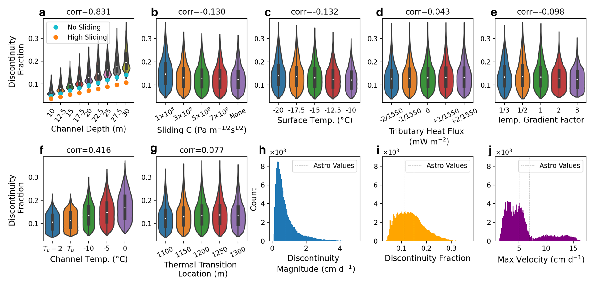
The velocity range, as opposed to the velocity maximum, is used in calculating the discontinuity fraction as it removes any component of plug flow, thus allowing a direct comparison between polythermal and temperate glacier simulations. For the polythermal glaciers discussed here, the velocity range is equivalent to the maximum velocity and using the velocity range has no effect on the discontinuity fraction.
The modeled glaciers produce discontinuity fractions ranging from 0.040 to 0.370 with a mean of 0.137 (Fig. 10). For reference, the observed discontinuity fraction across the Astro Channel is ~0.13. These fairly substantial discontinuity fractions are, themselves, a key result. They demonstrate that it is possible to achieve non-negligible discontinuous surface velocity fields such as those observed across the Astro Channel in the absence of ice fracture or highly specific thermal structures or sliding behaviors. The occurrence of cross-channel velocity discontinuities in the absence of ice fracture is in line with other work (e.g., Moore and others, Reference Moore, Iverson and Cohen2010; Monz and others, Reference Monz, Hudleston, Cook, Zimmerman and Leng2022) that casts doubt on ice fracture being responsible for structures attributed to thrust faulting. Indeed, the modeling shows that a fairly wide range of thermal structures and channel depths should give rise to discontinuous velocity fields detectable by high-resolution remote sensing.
Several factors related to the discontinuity fraction distributions shown in Figures 10a–g should be noted. First, channel depth is the only single variable that has a strong control on both the minimum and maximum discontinuity fraction. With all other variables, the maximum discontinuity fraction may change with variable choice but the minimum discontinuity fraction remains close to zero. This change in maxima only is most pronounced for the channel temperature, in which cold channels limit the maximum discontinuity fraction more strongly than their warm counterparts. A similar, albeit weaker, phenomenon occurs with the bed friction parameter C, surface temperature and temperature gradient factor.
Temperate glaciers
We model temperate glaciers with channel depths of D c (see Table 1). For each channel depth, the temperate discontinuity fractions (see Fig. 10a) closely bound (≤±16%) the smallest polythermal fractions for corresponding channel depths, while the temperate magnitudes (see Fig. S6) exceed the median of their polythermal counterparts by at least 20%. However, the smaller temperate discontinuity fractions are due to the comparatively large surface velocities of the temperate glaciers, as opposed to small cross-channel velocity discontinuities.
Model limitations
The cross-sectional nature of the ice-flow model discussed above results in several shortcomings, notably it neglects the longitudinal compression that results in measurable emergence velocities and inherently assumes that the glacier geometry (including the supraglacial channel) and thermal structure are longitudinally uniform. These geometric assumptions imply that the modeled supraglacial channel is infinitely long and perfectly straight, resulting in a discontinuity maximizing scenario as compared to channels that exhibit overall curvature or sinuosity. While channel curvature or sinuosity should reduce the discontinuity magnitude for a given set of model parameters, it is unclear how substantial the impact will be.
However, the largest shortcoming of the ice-flow model used above is not related to its cross-sectional nature but instead results from the lack of thermomechanical coupling. For the modeled glaciers, the thermal structure is simply generated by solving a heat diffusion equation over the model domain using boundary conditions that are loosely based on the climate of the study site. This method of generating thermal structures greatly reduces the complexity and computational cost of the model but fails to account for the thermal effects of ice advection and strain heating. A key result of the missing advection is that the temperature gradient with depth resulting from the heat diffusion equation is always linear and must be rescaled with a temperature gradient factor in order to achieve the depth-varying temperature gradients found in real glaciers. The lack of strain heating will impact the thermal structure, and thus the velocity field, throughout the glacier. At the discontinuity itself, where deformation rates are quite high, lack of strain heating and its ice-softening effects may cause the model to underestimate the magnitude of the velocity discontinuity when compared to a thermomechanically coupled model. However, rough estimates show that the influence of strain heating is much too small to cause any potential positive feedback loop that may lead to thermomechanical runaway. For the fastest modeled (i.e., highest slip) glaciers here, maximum strain heating rates are ~4000 J m−3 d−1, and only occur in a small volume directly beneath the channel. This energy is sufficient to melt ~14 g m−3 of temperate ice, leading to a negligible increase in interstitial water, and thus negligible changes in A.
While the lack of thermomechanical coupling yields less accurate glacier velocity fields, the simplicity and therefore low-computational cost of the model allows for testing a large number of model configurations. The large parameter space explored is useful, as many important model parameters such as channel depth, surface temperature and channel temperature are either unknown or poorly constrained. Moreover, as the modeling is intended to give a general understanding of ice flow across large supraglacial stream channels, the additional accuracy gained from thermomechanical coupling is not essential to the interpretation of model results.
Additional controls on A
Finally, we do not explicitly consider the possibility of water intrusion or strong single maximum fabrics in the ice around the channel. Both of these factors can substantially alter A (Duval, Reference Duval1977; Jacka and Budd, Reference Jacka and Budd1989; Adams and others, Reference Adams, Iverson, Helanow, Zoet and Bate2021) and may plausibly occur around water-filled supraglacial channels in areas undergoing high shear, such as the Astro Channel. Both interstitial water content and strong single maximum fabrics in simple shear should only serve to increase A, leading to a similar qualitative effect as high channel temperatures (i.e., an increase in discontinuity magnitude). As a point of reference, strong single maximum fabrics can result in an increase in A by up to a factor of 9 (Jacka and Budd, Reference Jacka and Budd1989; Jun and others, Reference Jun, Jacka and Budd1996), an impact similar to increasing ice temperature from $2.5$ to 0°C. Similarly, an increase in interstitial water content from 0 to 1.1% will lead to a threefold increase in the value of A (Duval, Reference Duval1977). Such values exceed those included in our model.
Discussion
Discontinuity causing channel geometry
The modeling results indicate that cross-channel velocity discontinuities substantial enough to be measured by high-resolution remote sensing or in situ methods can occur under a wide variety of thermal conditions (including in temperate glaciers) and sliding behaviors, and do not require implausibly deep supraglacial channels. However, observations of these cross-channel velocity discontinuities remain rare to date. The lack of observations likely occurs for two reasons. First, researchers are simply not measuring velocity fields across supraglacial channels using in situ methods. In addition, remote sensing that happens to image areas in which cross-channel velocity discontinuities occur will likely be unable to resolve the discontinuities unless a high-resolution sensor is used. The sensor resolution necessary to detect a cross-channel discontinuity will depend on the temporal baseline and discontinuity magnitude, but a sensor capable of resolving glacier motion of ~1 cm d−1 is a reasonable estimate. Furthermore, significant spatial smoothing, which is commonly performed on remotely sensed glacier velocity fields, will likely obscure any discontinuous motion.
Second, and more importantly, for supraglacial channels to form discontinuous motion fields, specific geometric requirements must be met. As the local transverse velocity gradient is proportional to the discontinuity fraction and magnitude (see Fig. S7), the channel must be positioned in a region of substantial lateral velocity gradients (and thus shear stresses) that are sustained over fairly long (likely kilometer-scale) distances. This means that the channel must be long and located in a band near the glacier margin where high shear stresses occur and run approximately parallel to the glacier flow direction. Channel depth also plays an important role, with model results indicating that as channels become shallower, an increasingly small number of parameter combinations give rise to substantial discontinuities. Defining a depth threshold for substantial discontinuous motion would require knowledge of glacier-specific properties such as thermal structure and sliding behavior. Supraglacial channels that meet these length and position criteria appear uncommon, but are more likely to occur on polythermal glaciers, which tend to have fewer drainage features such as moulins compared to their temperate counterparts (Bingham and others, Reference Bingham, Nienow and Sharp2003) and thus longer supraglacial streams and channels.
Moreover, to form channels of sufficient depth, very high incision rates or perennial occupation by meltwater are necessary. On polythermal glaciers, perennial occupation by meltwater appears necessary as anomalously high incision rates compared to those that have been observed would be necessary to form channels of 10 + m depth in a single melt season (Irvine-Fynn and others, Reference Irvine-Fynn, Hodson, Moorman, Vatne and Hubbard2011; St Germain and Moorman, Reference St Germain and Moorman2019). On temperate glaciers, where incision rates are generally higher than those found on polythermal glaciers, even when compared to the local ablation rates, it may be possible to form sufficiently deep channels in a single melt season with very high but still plausible incision rates (Ferguson, Reference Ferguson1973; Isenko and others, Reference Isenko, Naruse and Mavlyudov2005). However, some research indicates that the high discharge rates necessary to cut these channels in temperate glaciers are correlated with high sinuosity which would likely inhibit the velocity discontinuity by reducing the longitudinally averaged channel depth (Ferguson, Reference Ferguson1973; St Germain and Moorman, Reference St Germain and Moorman2019). Perennially occupied supraglacial channels, which may result in deep channels with lower sinuosity due to their lower discharge rates, are unlikely to form on temperate glaciers as high deformation rates would close the channel between melt seasons (Hambrey, Reference Hambrey1977; Irvine-Fynn and others, Reference Irvine-Fynn, Hodson, Moorman, Vatne and Hubbard2011). Alternatively, if a velocity discontinuity across a sinuous supraglacial channel does occur, the differential motion may cause the channel to pinch itself shut as one bank of the channel migrates into the other, provided the velocity discontinuity is greater than the rate at which the stream incises into the ice. In sum, the probability of a supraglacial channel meeting the length, depth and direction criteria necessary to cause a surface velocity discontinuity are small, with the most likely scenario occurring when perennial supraglacial streams form on polythermal glaciers.
Thompson Glacier channels
All three channels (i.e., Astro, West and Upper channels) on Thompson Glacier at which interferograms indicate the presence of discontinuous motion appear to match the length, depth and direction criteria to a degree. These three channels are large enough to appear prominently in satellite imagery, likely indicating that they are at least several meters deep although the Astro Channel appears wider, and thus probably deeper, than the Upper and West channels. All three channels are also approximately aligned with the direction of glacier flow for 2+ km. In the case of the Upper Channel, the distance from the glacier margin is ~400 m, similar to that of the Astro Channel, with the transverse velocity gradients, as measured by speckle tracking, being approximately twice as large as those in the vicinity of the Astro Channel. However, speckle tracking is unable to resolve a velocity discontinuity across the Upper Channel, indicating a cross-channel velocity difference of ≲0.5 cm d−1. This comparatively small velocity discontinuity, despite the larger transverse velocity gradient, is most easily explained as the result of a shallower channel depth. The West Channel is located ~900 m from the glacier margin, with transverse velocity gradients that are ~10% of those at the Astro Channel. Again, speckle tracking is unable to resolve a velocity discontinuity across this channel, indicating a cross-channel velocity difference of ≲0.5 cm d−1. This comparatively small velocity discontinuity could result from a combination of low shear stresses across the West Channel, as indicated by the transverse velocity gradients, and shallower channel depths.
Controls on channel formation and geometry
The three supraglacial channels on Thompson Glacier where discontinuous motion is detected originate at glacier confluences and are fed by marginal lakes, likely indicating meltwater occupation for part of the year. We speculate that channels conducive to discontinuous glacier motion may form preferentially at glacier confluences due to structural controls imposed by the two flow units. From optical satellite imagery we discern, qualitatively, that many glaciers on Umingmat Nunaat (Axel Heiberg Island) have long, flow-parallel supraglacial channels that originate at glacier confluences. Some, but not all, of these channels appear to be fed by ice-marginal lakes. Relatively little is known about what controls the location of supraglacial stream formation, however Hambrey (Reference Hambrey1977) has suggested that glacier structures, including flow units, may play some role in determining the location of small supraglacial streams. Moreover, Hambrey (Reference Hambrey1977) observed that many of these small streams follow structural features and, as a result, are often fairly straight. At a glacier confluence troughs may form between the two flow units (Glasser and Gudmundsson, Reference Glasser and Gudmundsson2012) which could create a structural feature that may potentially be exploited by water to form a long, flow-flowing supraglacial stream. Any shearing that occurs between two flow units will serve to preferentially align existing surface features, including supraglacial channels or troughs, with the flow direction. This, combined with the fact that asymmetric glacier (i.e., glaciers of mismatched size) confluences are likely to form a zone of high shear, may preferentially lead to formation and persistence of channels, located in zones of high shear, that have geometries conducive to discontinuous glacier motion.
The bed topography presents another potential control on channel formation. We do not model such scenarios owing to limited information about the bed of Thompson Glacier, but the most relevant scenario here would be a topographic step underlying the Astro Channel. Such a step could potentially fix the location of a slip-to-no-slip transition at the bed which may then cause preferential erosion under the thawed central portion of the bed (Cook and others, Reference Cook, Swift, Kirkbride, Knight and Waller2020), leading to an increase in step size. If such a step exists, the sharp difference in ice thickness and thermal structure across the Astro Channel would likely increase the size of any velocity discontinuity for a given set of parameters.
Conclusion
High-resolution SAR speckle tracking of glaciers remains largely underleveraged but may be broadly useful to measure and investigate mesoscale (multi-centimeter) glacier motion. In this study, we use high-resolution speckle tracking to investigate mesoscale discontinuous motion, initially detected by InSAR, across supraglacial stream channels on Thompson Glacier, Umingmat Nunaat (Axel Heiberg Island). To improve the accuracy of our speckle tracking, we develop and use an intensity prefilter designed to reduce false matches. We then use a 2-D cross-sectional ice-flow model to investigate the controls on discontinuous glacier motion similar to that observed on Thompson Glacier.
As the magnitude of the velocity discontinuities on Thompson Glacier are small (several cm d−1), spatial smoothing of the speckle tracking results, as is commonly done to reduce errors, obscures the discontinuities. Instead, we analyze the possible causes of speckle tracking errors and find that false matches often occur when speckle tracking locks-on to high-intensity pixels, which in SAR images of glaciers, are often structural features such as crevasses or stream channels. To improve SAR speckle tracking performance, we use a SAR simulator capable of generating SLC pairs with a user-defined motion field to study optimum intensity rescaling as a pre-conditioning step. The intensity-rescaled speckle tracking is then used to measure the motion of the Expedition Fjord area glaciers.
The measured glacier speeds compare well (MAE of 0.52 cm d−1) to annual speeds from NASA ITS_LIVE data, a lower resolution global glacier motion dataset. Interferograms indicate that cross-channel discontinuous motion is occurring along three supraglacial channels on Thompson Glacier. However, only at the Astro Channel the magnitude of the velocity discontinuity is large enough to be resolved by the speckle tracking results, indicating that the discontinuity at the other two channels is ≲0.5 cm d−1. The remote sensing observations show an uncommon form of discontinuous glacier motion characterized by ice on the central (west) side of the Astro Channel flowing ~30% (1 cm d−1) faster than the ice immediately across the ~3 m wide channel.
A cross-sectional ice-flow model is used to investigate the physical causes of this discontinuous motion. The finite-element ice-flow model uses a domain inspired by Thompson Glacier that includes a surface channel similar to the Astro Channel. The modeling shows that discontinuous glacier motion of the form and magnitude observed across the Astro Channel can occur, without ice fracture and under a wide variety of plausible channel depths and thermal structures, including in temperate glaciers.
We also use the ice-flow model to investigate the sensitivity of the velocity discontinuity to various model parameters. Channel depth is the primary control on the velocity discontinuity, but low surface temperatures and high in-channel temperatures, caused in the real world by water flow within the channel, also contribute to larger cross-channel velocity discontinuities. Again, the modeling demonstrates that specific or unusual thermal structures are not necessary to cause cross-channel discontinuous motion, implying that the rarity of this form of motion is instead a result of the channel geometry. Namely, the channel must be deep, straight, flow-following and long, and located in areas of high lateral shear stress. We speculate that channels conducive to discontinuous motion form and persist preferentially on polythermal glaciers, particularly in the presence of glacier confluences and their associated ice-marginal lakes.
Supplementary material
The supplementary material for this article can be found at https://doi.org/10.1017/jog.2023.67
Acknowledgements
SFU, NSERC, CSA and MDA provided funding for this study. We thank MDA for their support in obtaining RADARSAT-2 data and acknowledge J. Eppler for helpful discussions on creating simulated SAR images. We are grateful to L. Thomson for providing advice, photographs and study-site specific knowledge. Finally, we thank B. Minchew and a second anonymous reviewer for their thorough and insightful comments.
Author contributions
B.R. broadly conceived of the remote sensing portion of this study with specifics determined by G.C. G.C. conceived of the glacier modeling portion with input from G.E.F and B.R. G.C. carried out both remote sensing and ice-flow analysis and modeling with guidance from B.R. and G.E.F. G.C. led manuscript preparation with advice and editing from B.R. and G.E.F.


 Open access