


1. INTRODUCTION
Patagonia is the largest ice-covered region in the Southern Hemisphere outside of Antarctica (Rignot and others, Reference Rignot, Rivera and Casassa2003). Most of the ice is locked in two main icefields: the Northern Patagonia Icefield (NPI 3976 km2) and the Southern Patagonia Icefield (SPI 13219 km2) (Davies and Glasser, Reference Davies and Glasser2012). Most Patagonian glaciers have been losing mass and retreating for the last 40 years (Aniya, Reference Aniya1999; Lopez and others, Reference Lopez2010; Casassa and others, Reference Casassa, Rodríguez and Loriaux2014). Estimations of total mass balance from different sources confirm the acceleration of mass losses in the last decades compared with mean value over the entire period since the Little Ice Age to present (Rignot and others, Reference Rignot, Rivera and Casassa2003; Glasser and others, Reference Glasser, Harrison, Jansson, Anderson and Cowley2011; Jacob and others, Reference Jacob, Wahr, Pfeffer and Swenson2012).
The NPI is located between 46.5°S and 47.5°S. It is under the influence of the westerlies (Garreaud and others, Reference Garreaud, Vuille, Compagnucci and Marengo2009) and climate settings are largely influenced by the Southern Annular Mode (Thompson and Wallace, Reference Thompson and Wallace2000; Garreaud and others, Reference Garreaud, Lopez, Minvielle and Rojas2013). The westerly flow transports large amounts of moisture from the southern Pacific Ocean towards the continent. Air parcels are lifted upwards by convection over the Andes entailing orographic precipitation, leading to high precipitation with strong W-E gradients (Carrasco and others, Reference Carrasco, Casassa and Rivera2002; Garreaud and others, Reference Garreaud, Lopez, Minvielle and Rojas2013). NPI's climate is thus temperate and very humid, with precipitation exceeding 10 m w.e. in the highest zone (Garreaud and others, Reference Garreaud, Lopez, Minvielle and Rojas2013). The equilibrium line altitude (ELA) is located ~950–1300 m a.s.l. (Rivera and others, Reference Rivera, Benham, Casassa, Bamber and Dowdeswell2007). This elevation band comprises a flat and vast plateau, making the icefield surface mass balance particularly sensitive to shifts in the ELA in response to changes in temperature and accumulation. The NPI is formed by 140 units in the RG inventory, including 38 main glaciers of different terminus types: one tidewater calving glacier (San Rafael Glacier (SRG) covering 18% of the total surface area), 18 fresh water calving glaciers (64% of the total surface area) and 19 land-terminating glaciers (18% of the surface area) (Rivera and others, Reference Rivera, Benham, Casassa, Bamber and Dowdeswell2007; Willis and others, Reference Willis, Melkonian, Pritchard and Rivera2012; Pfeffer and others, Reference Pfeffer2014). A recent ice velocity mosaic reveals that fast flow regions extend far into the plateau and accumulation area, making the icefield also potentially sensitive to dynamical changes (Mouginot and Rignot, Reference Mouginot and Rignot2015).
This study focuses on SRG, located in the north-western part, and the largest glacier of NPI with an area of 734 km2 (Fig. 1). It covers the entire altitude range of the NPI: the highest point of the glacier catchment is the San Valentin peak at 4032 m a.s.l. (Vimeux and others, Reference Vimeux2008) and it ends at sea level in the Laguna San Rafael. Laguna San Rafael is connected to the Pacific Ocean through Témpanos River and Elefantes Fjord. From remotely sensed snowlines and surface mass balance modelling studies, the ELA has been estimated between 905 and 1295 m a.s.l. (Aniya, Reference Aniya1988; Rignot and others, Reference Rignot, Forster and Isacks1996; Rivera and others, Reference Rivera, Benham, Casassa, Bamber and Dowdeswell2007; Koppes and others, Reference Koppes, Conway, Rasmussen and Chernos2011; Schaefer and others, Reference Schaefer, Machguth, Falvey and Casassa2013). SRG is among the fastest glaciers in the world with frontal velocities exceeding 7 km a−1 (Willis and others, Reference Willis, Melkonian, Pritchard and Rivera2012; Mouginot and Rignot, Reference Mouginot and Rignot2015). The terminus position has retreated by more than 10 km since the end of the Little Ice Age in 1870. Since 1990 the retreat has slowed down and since the early 2000s the terminus has been maintained in a nearly stable position in a narrow 2 km wide valley (Davies and Glasser, Reference Davies and Glasser2012).
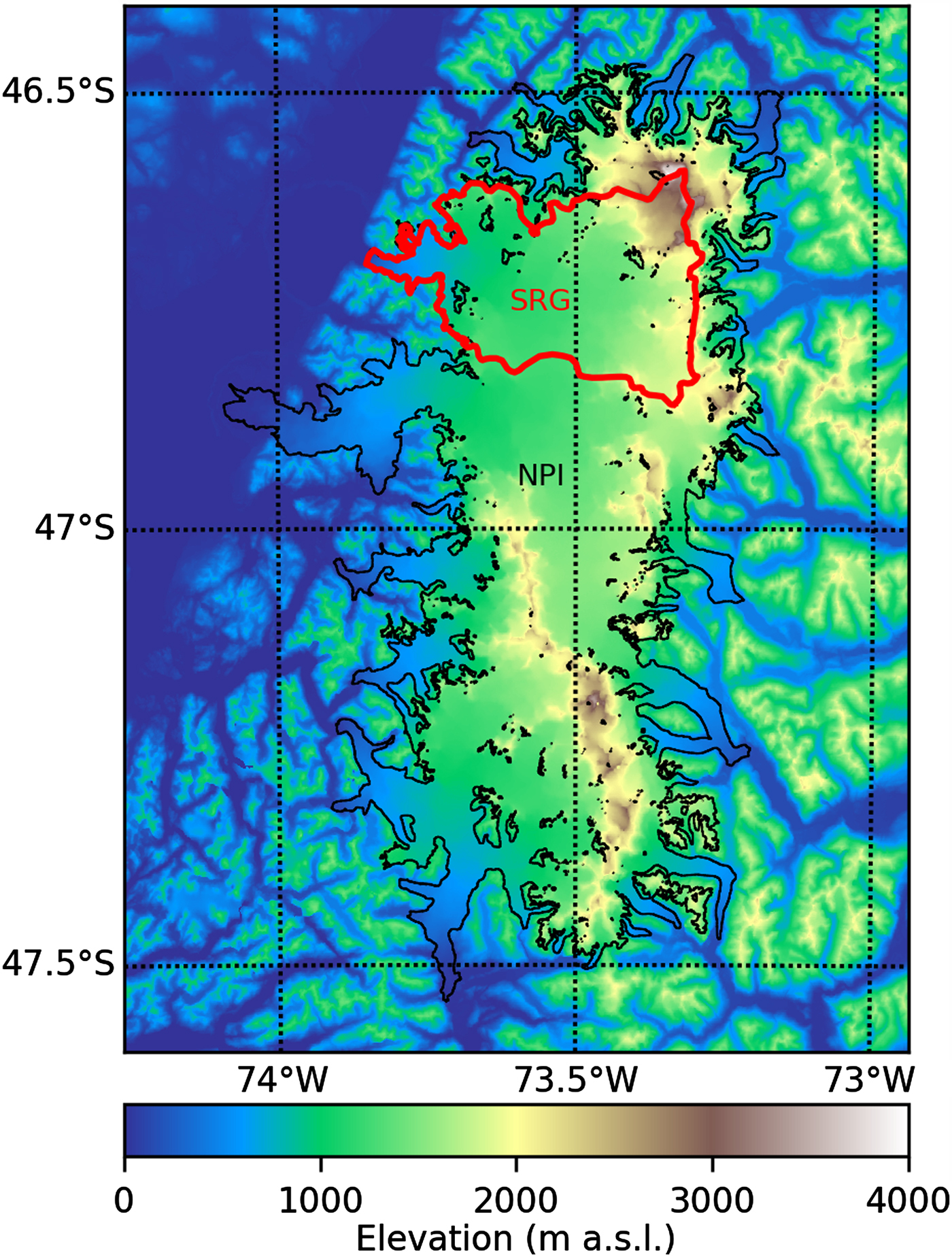
Fig. 1. Map of the surface elevation of our study area. In black, the outline of the Northern Patagonia Icefield (NPI) from Rivera and others (Reference Rivera, Benham, Casassa, Bamber and Dowdeswell2007). In red, the outline of San Rafael Glacier (SRG) from Mouginot and Rignot (Reference Mouginot and Rignot2015). Elevations from SRTM-2000. Datum WGS84.
Neglecting volume changes due to advance or retreat of the glacier front and melting at the base in contact with the bed, the total mass balance ( $\dot M$) of a calving glacier results from the difference between the surface mass balance ( $\dot B$) and the ice discharge ( $\dot D$), i.e. $\dot M = \dot B - \dot D$. $\dot M$ and $\dot D$ can be estimated from remote-sensing observations: the total mass balance can be derived from the volumetric change obtained from surface elevations changes measured, for example, by differencing DEMs. Between 2001 and 2011, SRG has been losing volume at a rate of −0.82 ± 0.06 km3 a−1 (−4.06 ± 0.11 km3 a−1 for the entire NPI) (Willis and others, Reference Willis, Melkonian, Pritchard and Rivera2012). The ice discharge is usually estimated by combining thickness and surface velocity observations. Using surface velocities derived from a 7-day interval pair of ASTER images in the austral fall 2007 and an estimate of the calving front vertical area (from bathymetry measurements (Koppes and others, Reference Koppes, Conway, Rasmussen and Chernos2011), Willis and others (Reference Willis, Melkonian, Pritchard and Rivera2012) calculated $\dot D$ = −2.22 km3 a−1, a value 60% greater than previous estimates for 1994 (−1.7 km3 a−1) (Rignot and others, Reference Rignot, Forster and Isacks1996). However, SRG surface velocities from Mouginot and Rignot (Reference Mouginot and Rignot2015) do not show a clear temporal trend, except a slight deceleration (20%) after a maximum in 2005 (15% above the 1994 value), at 9 km from the front. $\dot B$ is usually estimated by downscaling reanalysis data with more or less complex models (Koppes and others, Reference Koppes, Conway, Rasmussen and Chernos2011; Schaefer and others, Reference Schaefer, Machguth, Falvey and Casassa2013; Lenaerts and others, Reference Lenaerts2014). Schaefer and others (Reference Schaefer, Machguth, Falvey and Casassa2013) found a clearly positive $\dot B$ of 1.6 m w e. for 1979–2011. Using the catchment area (734 km2) this corresponds to a $\dot B$ value of 1.17 km3 a−1 of ice, which is larger than the 0.71 km3 a−1 positive value of ice given by Koppes and others (Reference Koppes, Conway, Rasmussen and Chernos2011) for 1960–2005. Schaefer and others (Reference Schaefer, Machguth, Falvey and Casassa2013) and Lenaerts and others (Reference Lenaerts2014) suggest that $\dot B$ over the whole NPI has been increasing since the 1980s. Koppes and others (Reference Koppes, Conway, Rasmussen and Chernos2011) also found that $\dot B$ over SRG has increased from −0.29 ± 0.21 km3 a−1 for the period 1977–89 to 0.79 ± 0.41 km3 a−1 for the period 1990–2005. The increase in $\dot B$ seems in contradiction to the unabated rates of mass loss. Thus, these previous studies proposed that, the increasing $\dot B$ has been compensated by increased ice discharge. However, this is in contradiction with the lack of significant variations in observed velocities by Mouginot and Rignot (Reference Mouginot and Rignot2015). Further, the absolute value of $\dot B$ and its temporal changes are poorly constrained for several reasons: (1) due to the remoteness of the area and the harsh climatic conditions, no long-term meteorological data close to the icefield are available to perform a rigorous climatic study, comprising the reliability of reanalysis products over Patagonia (Nicolas and Bromwich, Reference Nicolas and Bromwich2010). Moreover, climatic trends in this region are largely impacted by assimilation of satellite datasets in 1979 (Kistler and others, Reference Kistler2001; Uppala and others, Reference Uppala2005). (2) Direct surface mass-balance measurements are scarce on NPI and particularly at high elevations (>1000 m a.s.l.) impeding a full validation of the accumulation simulated by the models.
Here we explore a new approach using a physically-based ice flow model to constrain SRG surface mass balance. First, the model is calibrated using available data of surface velocity and rate of surface elevation change for the period 2000–12. Then, running the model forward in time enables the selection of  $\dot B$ values that are compatible with modelled ice fluxes. Finally, the model is used to simulate the diffusion of the observed thinning and to estimate the committed mass loss induced by the current glacier imbalance.
2. DATA AND PREVIOUS ESTIMATIONS
2.1. Surface mass balance
In this section, we present the initial point surface-mass balance functions ( $\dot b$) used to force our ice flow model. They are obtained from previous studies results (Koppes and others, Reference Koppes, Conway, Rasmussen and Chernos2011; Schaefer and others, Reference Schaefer, Machguth, Falvey and Casassa2013). First, we describe the methodology from these two studies, analyze their difference and uncertainties and compare with in situ measurement available in the literature. Afterwards we describe how we obtain the initial $\dot b$ functions and the additional function that we explore.
Schaefer and others (Reference Schaefer, Machguth, Falvey and Casassa2013) used the Weather Research and Forecasting (WRF) regional circulation model forced with data from the NCAR/NCEP reanalysis over the period 2005–11. These results are used to build a statistical downscaling method to downscale the reanalysis from 1975 to 2011. Finally, a distributed mass-balance model with a degree-day approach was applied. The downscaling results (temperature, precipitation and incoming solar radiation) were validated with data from 16 weather stations located at low elevations (<427 m) around the icefield. The modelled mean surface mass balance of the entire NPI was calibrated using geodetic mass-balance data from the three largest noncalving glaciers (HPN-1, HPN-4 and Exploradores) and with point surface mass-balance measurements. These three glaciers presented negative  $\dot B$ which were well captured by the model. However, these glaciers have small accumulation areas and they do not necessarily represent what happens in the plateau where most of the accumulation in NPI and SRG takes place. The point surface mass-balance measurements were given by 18 ablation stakes below 1200 m a.s.l. (Ohata and others (Reference Ohata, Ishikawa, Kobayashi and Kawaguchi1985) and taken by Centro de Estudios Científicos (CECs), Valdivia, Chile) and two values from the accumulation area obtained by analysing shallow firn cores (Yamada, Reference Yamada1987; Matsuoka and Naruse, Reference Matsuoka and Naruse1999). Thus, in general, the model results were not well calibrated in the accumulation zone. Schaefer and others (Reference Schaefer, Machguth, Falvey and Casassa2013) suggested that the $\dot B$ over NPI slightly increased between 1975 and 2011. During this period, the $\dot B$ of the SRG was strongly positive with a mean glacier-wide surface mass balance of 1.6 m w.e. a−1 (1.19 km3 a−1 with ice density of 910 kg m−3). At the glacier snout, point surface mass balance was as negative as −14.3 m w.e. a−1, whereas the maximum was found at the top of the San Valentin peak with 20.8 m w.e. a−1. The mean ELA is found to lie at 1203 m a.s.l. The very high accumulation at the San Valentin peak, however, disagrees with the drastically lower values obtained through an ice core (0.2 m w.e. a−1; Vimeux and others, Reference Vimeux2008). Even though the mean accumulation given by the ice core may be site-specific, this difference between observation and model gives low confidence in the accumulation obtained by Schaefer and others (Reference Schaefer, Machguth, Falvey and Casassa2013).
On the other hand, Koppes and others (Reference Koppes, Conway, Rasmussen and Chernos2011) estimated the  $\dot B$ between 1960 and 2005 using a downscaling of NCEP/NCAR reanalysis data based on correlations between reanalysis data at a gridpoint and daily precipitation and temperature measured over 1 year by a weather station installed on the shores of Laguna San Rafael ~7 km from the glacier front. To reconstruct the temperature profile over the entire glacier they used daily lapse rates computed from NCEP/NCAR reanalyses. To reconstruct precipitation, they used the corrected precipitation and an orographic enhancement factor estimated from a simplified 1-D orographic precipitation model (Smith and Barstad, Reference Smith and Barstad2004; Roe, Reference Roe2005). To estimate the ablation amounts, they used a PDD model calibrated for ice with the ablation stake measurements from Ohata and others (Reference Ohata, Ishikawa, Kobayashi and Kawaguchi1985) and a PDD factor for snow estimated by Hock (Reference Hock2003). Hence, as in the previous study, the model was only calibrated in the ablation zone. They proposed a positive average $\dot B$ of 0.71 km3 a−1 for the entire period (1960–2005) with three sub-periods of very positive (1.4 km3 a−1 in 1960–76), negative (−0.29 km3 a−1 in 1977–89) and positive (0.79 km3 a−1 in 1990–2005) surface mass balance. The point surface mass balance as a function of surface elevation is shown in Figure 2a; it increases from ~−16.2 m a−1 w.e. at sea level to a maximum of 7.8 m a−1 w.e. at 1800 m a.s.l. Above this maximum, $\dot B$ decreases to 3 m a−1 w.e. at 4000 m a.s.l. (estimated from Koppes and others (Reference Koppes, Conway, Rasmussen and Chernos2011)).
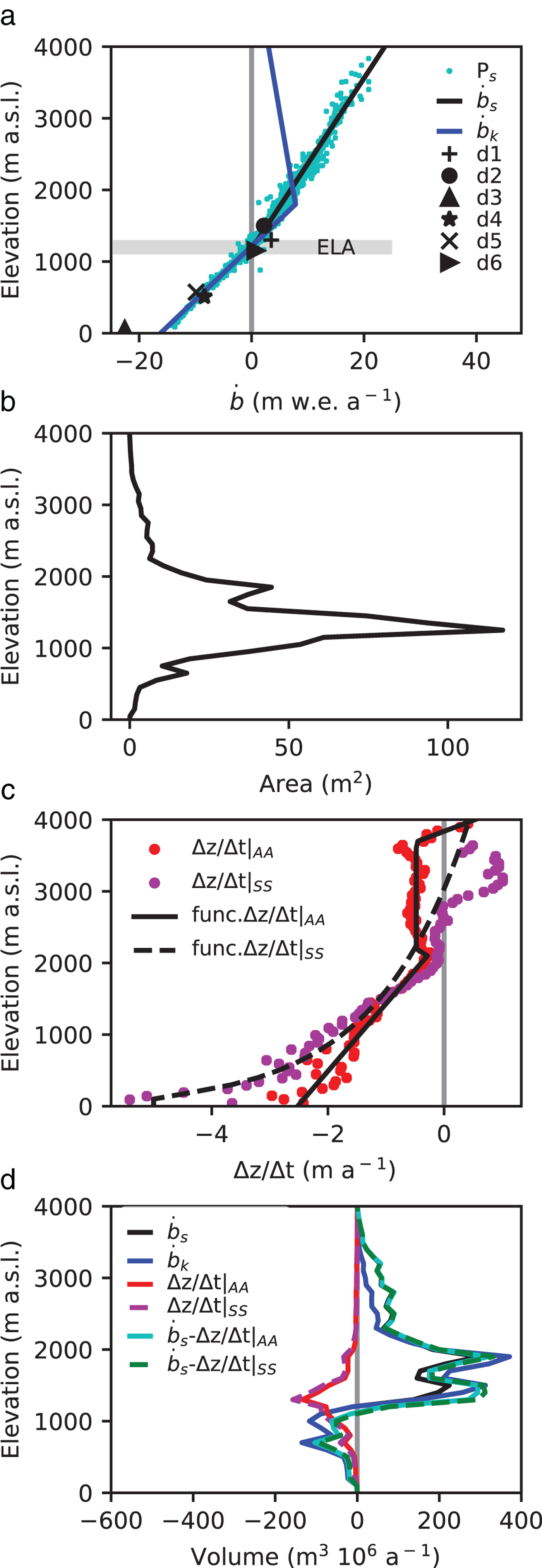
Fig. 2. (a) Distribution of the surface mass balance ( $\dot b$) from different sources as a function of elevation. P S correspond to the point surface mass-balance model outputs from Schaefer and others (Reference Schaefer, Machguth, Falvey and Casassa2013) for SRG, $\dot b_{\rm s} $ is a piece-wise linear regression to these data, $\dot b_{\rm k} $ is mean surface mass-balance function of SRG from Koppes and others (Reference Koppes, Conway, Rasmussen and Chernos2011), represented as a piece-wise linear function and obtain from their Figure 8. d1 to d6 are the observed $\dot b$ on NPI and listed in Table 1. (b) SRG hypsometry from the SRTM-2000. (c) Surface elevation change in SRG from the two different space-borne geodetic methods (AA and SS, see text) and (d) $\dot b$ functions and surface elevation changes expressed in volume according to elevation for the two different sources (AA and SS).
We compare the point surface mass-balance ( $\dot b$) field measurements of SRG with these two model estimations: the average between 1975 and 2011 from Schaefer and others (Reference Schaefer, Machguth, Falvey and Casassa2013) and the average between 1960 and 2005 from Koppes and others (Reference Koppes, Conway, Rasmussen and Chernos2011). In the ablation zone, there is an agreement between measurements and models. However, in the accumulation zone, there is a lack of measurements and results from both studies present strong discrepancies (Fig. 2a and Table 1). Koppes and others (Reference Koppes, Conway, Rasmussen and Chernos2011) proposed a lower $\dot B$ than Schaefer and others (Reference Schaefer, Machguth, Falvey and Casassa2013) and took into account a maximum elevation above which the precipitation decreased. However, the lower $\dot B$ value in Koppes and others (Reference Koppes, Conway, Rasmussen and Chernos2011) was not only due to this maximum, but also to the hypsometry of SRG (Fig. 2b) and more particularly around the ELA (between 1000 and 1400 m a.s.l.), where most of the glacier area is concentrated (52% of the area).
Table 1. Published point surface mass-balance measurements over the Northern Patagonia Icefield

Based on these earlier studies, we define two drastically different altitudinal distributions of  $\dot b$ to force our ice flow model of SRG. We use the mean annual mass-balance function for the period 1960–2005 given by Koppes and others (Reference Koppes, Conway, Rasmussen and Chernos2011, Fig. 8), to define the following functions:
 $$\eqalign{& \dot b_{\rm k} (z_{\rm s} ) = 0.013z_{\rm s} - 16.2\quad {\rm if}\,z_{\rm s} \le 1800 \cr & \dot b_{\rm k} (z_{\rm s} ) = - 0.0022z_{\rm s} + 11.7\quad {\rm if}\,z_{\rm s} \gt 1800} $$
 From Schaefer and others (Reference Schaefer, Machguth, Falvey and Casassa2013),  $\dot b$ is approximated using two linear relationships, below and above the ELA, following the Area Altitude Balance Ratio method (Osmaston, Reference Osmaston2005). Using the averaged for the period 1975–2011 (see Fig. 2a), we use:
 $$\eqalign{& \dot b_{\rm S} (z_{\rm s} ) = 0.013z_{\rm s} - 16.2\quad {\rm if}\;z_{\rm s} \le 1200 \cr & \dot b_{\rm S} (z_{\rm s} ) = 0.0084z_{\rm s} - 9.8\quad {\rm if}\;z_{\rm s} \gt 1200} $$
 Both altitudinal distributions of  $\dot b$ coincide in the ablation zone. While the values given by Koppes and others (Reference Koppes, Conway, Rasmussen and Chernos2011) and Schaefer and others (Reference Schaefer, Machguth, Falvey and Casassa2013), cover slightly different time periods because they are averaged over a period longer than 30 years, we expect that they are a good approximation of a mean local climatology for the last decades.
In addition to these two altitudinal functions of  $\dot b$, we explored different surface mass-balance trends with elevation to find a $\dot b$ function consistent with the initial ice flow dynamics. As surface mass balance is well constrained below the ELA, we only vary the $\dot b$ parametrization in the accumulation zone.
2.2. Glacier geometry
The glacier hypsometric curve as given by the SRTM-2000 DEM is shown in Figure 2b. The glacier has a uni-modal area distribution where most of the area is found in the plateau between 1000 and 2000 m a.s.l. The maximum of the area is at an altitude of 1250 m a.s.l., i.e. close to the ELA.
The glacier drainage basin delineation is taken from Mouginot and Rignot (Reference Mouginot and Rignot2015). They used their surface velocity data to define the ice divide over the plateau where the surface slope is too small to accurately define the divide.
The ice thickness and bedrock topography have been obtained from airborne gravity data (Gourlet and others, Reference Gourlet, Rignot, Rivera and Casassa2016). The maximum estimated error is between 38 and 64 m on the NPI plateau and reaches 114 m in the narrow valleys.
2.3. Volume changes related to surface elevation change
The surface elevation change between 2000 and 2012 (Δz s/Δt) is calculated with the geodetic method using either multiple ASTER DEMs (Berthier and others, Reference Berthier, Cabot, Vincent and Six2016) or by simple DEM differencing applied to a pair of SPOT5 and SRTM DEMs (Gardelle and others, Reference Gardelle, Berthier, Arnaud and Kääb2013). Both results agree within errors bars with a mean volume change of −0.80 ± 0.06 and −0.92 ± 0.07 km3 a−1, respectively. This is also consistent with the value of −0.82 ± 0.06 km3 a−1 from Willis and others (Reference Willis, Melkonian, Pritchard and Rivera2012) for the period 2001–11. The rates of surface elevation changes averaged by 50 m altitude bands are shown in Figure 2c. Data are thereafter denoted according to their origin as Δz s/Δt|AA for the multiple ASTER DEMs and Δz s/Δt|SS for the pair of SPOT5 and SRTM DEMs. There is a good agreement between both datasets between 1000 and 2000 m a.s.l. where most of the SRG area lies, while the two datasets differ outside of this range. Δz s/Δt|AA leads to lower thinning rates below 1000 m a.s.l., with a minimum of −2.5 m a−1 close to the glacier front (−5.0 m a−1 for Δz s/Δt|SS). They also show a slight trend to thinning in the upper reaches. However, due to the hypsometry of the glacier, the volume change is concentrated around 1200 m a.s.l. (Fig. 2d).
2.4. Surface velocities
Surface velocities are derived from SAR and Landsat satellite data using a speckle tracking algorithm, interferometric phase of ascending and descending tracks and feature tracking (Mouginot and Rignot, Reference Mouginot and Rignot2015). For best coverage, we use the velocity mosaic from imagery acquired between 1994 and 2014. The mosaic is mostly representative for the dynamic regime in 2004. As no significant trend has been observed in the surface velocities between 2000 and 2012, we consider the mosaic representative for this time interval (Fig. 3a). The maximum uncertainty reported here is computed as the 1 sigma error of the distribution of absolute displacement in ice-free areas, and it is 52 m a−1 for point velocities.

Fig. 3. (a) Observed surface velocities mosaic 1994–2014 and mostly representative of ice surface conditions in 2004 (Mouginot and Rignot, Reference Mouginot and Rignot2015). (b) Modelled surface velocities. (c) Relative error and (d) Histogram of the relative velocity error (%). White and black contour lines correspond to surface velocities contours (0.1 and 1.0 km a−1).
3. METHODS
This section describes the methodology in two main steps: the ice flow model initialization and prognostic simulations. For the model initialization, we first use an inverse method to constrain the distribution of basal friction using the observed surface velocities. Thereafter, we relax the model using an apparent surface mass balance using the observed surface elevation changes and different  $\dot b$ functions. We discard the simulations for which the volume changes exceed the surface elevations changes uncertainty. Afterwards, we check that the simulated velocities and surface elevations changes are close to the observation. As the observations used to constrain the model have been collected mostly between 2000 and 2012, after the initialization, we assume that the model state is representative of this period (study period). Finally, we run 100 years of prognostic simulations using constant forcing to estimate the committed mass loss induced by the initial model imbalance.
3.1. Model description
To model SRG flow-dynamics, we use the finite-elements full-Stokes 3-D ice flow model Elmer/Ice. Details on the numerical methods and model capabilities can be found in Gagliardini and others (Reference Gagliardini2013). Hereafter, we briefly outline the main assumptions used in our study.
To compute the velocity, u = (u i, u j, u k), we solve the 3-D Stokes equations that comprise the conservation of linear momentum and mass. For the rheological law, we use the nonlinear isotropic Glen's flow law, which links the deviatoric stress tensor τ with the strain-rate tensor ε as follows:
 $$\tau _{{\rm ij}} = 2\eta \dot \varepsilon_{{\rm ij}} $$
The effective viscosity (η) is equal to:
 $$\eta = \displaystyle{1 \over 2}(A)^{ - 1/n} \dot \varepsilon _{\rm e} ^{(1 - n)/n} $$
where n is the Glen exponent (taken here equal to 3) and  $\dot \varepsilon_{\rm e} = (\dot \varepsilon_{{\rm ij}} \dot \varepsilon_{{\rm ji}} /2)^{0.5} $ is the strain-rate second invariant. The rate factor A is a function of the temperature relative to the pressure melting point, following the Arrhenius equation. The values of all parameters are taken from Cuffey and Paterson (Reference Cuffey and Paterson2010).
The ice temperature is 0°C over the entire ice column between the front and the ELA (1200 m a.s.l. according to Schaefer and others, Reference Schaefer, Machguth, Falvey and Casassa2013). Above the ELA the thermal regime of the glacier is poorly constrained. Here we assume that the surface temperature varies linearly between 0°C at the ELA and −11.4°C at 3800 m a.s.l., in agreement with the only value given in the upper reaches (measured at 10 m depth by Vimeux and others, Reference Vimeux2008). We further assume that the ice temperature is uniform over the local ice column and correspond to the surface temperature. To assess the sensitivity of the model to this assumption we ran several initialization experiments assuming either that the glacier is temperate everywhere or that the temperature is the steady-state solution of the heat equation, with prescribed geothermal heat flux at the bottom boundary and temperature at the upper surface. In agreement with Seroussi and others (Reference Seroussi2013), we found that the model is weakly sensitive to the thermal regime in the upper zone. The results from all simulations represent the observed velocities with similar accuracy.
The 2-D footprint of the model domain, delineated by the red polygon in Figure 1, is meshed using the anisotropic mesh adaptation software Yams (Frey and Alauzet, Reference Frey and Alauzet2005). We use the geometric error estimate given by Frey and Alauzet (Reference Frey and Alauzet2005), which provides an upper bound for the interpolation error of a continuous field into piecewise linear elements. This error depends on the second spatial derivatives. The element size is then adjusted to equi-distribute the error over the whole domain. Here we use the observed surface velocities as the reference to estimate the error. The mesh resolution in 2-D ranges from 50 to 500 m. The 2-D mesh is then vertically extruded between the bottom and top surfaces using five layers. The thickness of the layer follows a geometric progression. The layer below the surface is two times thicker than the bottom layer. The ice thickness and the bedrock topography of the glacier are taken from Gourlet and others (Reference Gourlet, Rignot, Rivera and Casassa2016). The surface topography is estimated as the bottom topography plus the ice thickness.
We distinguish four different types of boundary conditions:
(1) At the bottom surface, the ice is in contact with the bed and we apply a linear friction law that relates the tangential basal shear stress (τ b) to the tangential sliding velocity (u b) as:
(5) $${\it \tau}_{\rm b} = \beta {\bi u}_{\rm b} $$
The friction coefficient β is inferred from observed surface velocities using a control inverse method as described in the following section. Normal to the bed (n), no outflow is allowed u.n = 0.
(2) At the upper surface (Γs), the ice is in contact with the atmosphere and is stress-free. The surface elevation is prescribed from the observation in the inverse method (steady state) but is free to evolve in the prognostic simulations following the kinematic equation:
(6)where z s = z s(x,y,t) is the surface elevation, us = (u s,i, u s,j, u s,k) is the surface velocity and$$\displaystyle{{\partial z_{\rm s}} \over {\partial t}} + u_{{\rm s},{\rm i}} \displaystyle{{\partial z_{\rm s}} \over {\partial x}} + u_{{\rm s},{\rm j}} \displaystyle{{\partial z_{\rm s}} \over {\partial y}} - u_{{\rm s},{\rm k}} = \dot b$$$\dot b$ is the surface mass balance given as a vertical flux.(3) At the calving front, the ice below sea level (z sl) is in contact with the water from the fjord, this leads to the following Neumann condition:
(7)where σ is the stress tensor, n is the unit vector in the normal direction, ρ w is the sea water density and g the norm of the acceleration due to gravity.$${\bi \sigma}. {\bi n} = \left\{ {\matrix{ { - \rho _{\rm w} g(z_{{\rm sl}} - z) \bi n} & {{\rm if}\quad \,z \le z_{{\rm sl}}} \cr {\bf 0} & {{\rm if}\quad \,z \gt z_{{\rm sl}}} \cr}} \right.$$(4) Lateral boundaries are taken from the drainage basin delineation and correspond either to artificial ice–ice boundaries in the upper reaches or ice–bed boundaries where the SRG flow is constrained by the topography. Both types are treated with the same conditions, assuming zero in or outflow (u.n = 0) in the normal direction n and free-slip in the tangential directions.


Ice volume changes result from the balance between incoming/outgoing ice fluxes into/from the model domain. Accurate computation of these fluxes is a pre-requisite for the computation of volume changes. Below we give details on the computation of the different fluxes.
The glacier-wide surface mass balance ( $\dot B_0 $) used to force the model is computed as the ablation/accumulation flux through the free surface Γs as:
 $$\dot B_0 = \int_{\Gamma _{\rm s}} {\dot b{\bi z} \cdot {\bi n}{\rm d}\Gamma} $$
where z is the unit vector in the vertical direction. Because the mesh must have a strictly positive thickness, the free surface equation (Eqn (6)) is solved with a constraint for the minimal surface elevation for each node, corresponding to a minimal thickness of 10 m. To satisfy this constraint, the model produces an additional mass flux that can be accurately quantified from the residual  $R_{Z_{\rm s}} $ of Eqn (6). The total mass flux through the upper free surface that corresponds to the corrected ( $\dot b$) is then given by:
 $$\dot B = \dot B_0 + R_{z_{\rm s}} $$
 This corrected glacier-wide surface mass balance ( $\dot B$) agrees with the ice flow and will be used hereafter as the glacier-wide surface mass balance.
Since the front is not a free surface, the ice discharge flux ( $\dot D$) is directly computed as:
 $$\dot D = \int_\Gamma {{\bi u}.{\bi n}{\rm d}\Gamma} $$
where Γ is the calving front boundary. As the terminus position is prescribed in the prognostic simulations, this corresponds to the calving flux required to keep a steady calving front location. During the study period the glacier front retreat was slow (220 m between 2000 and 2012, equivalent to 18 m a−1 and 0.004 km3 a−1) estimated from CECs and DGA (2012) and Mouginot and Rignot (Reference Mouginot and Rignot2015), suggesting that mass losses resulting from the glacier retreat were negligible in comparison with ice discharge. As discussed in Gillet-Chaulet and others (Reference Gillet-Chaulet2012), the nonpenetration condition at the bottom and lateral boundaries are enforced as a Dirichlet condition at the nodes, this may result in a nonnull ice flux computed through the boundary elements. Here, we use a definition of the nodal normals consistent with mass conservation so that, globally, the ice flux through the bottom and lateral boundaries is negligible.
The volume change over the model domain is then given by:
 $$\displaystyle{{{\rm d}V} \over {{\rm d}t}} = \dot B - \dot D$$
We verified that this relation is numerically satisfied within a limit of accuracy of 1% of dV/dt.
3.2. Model initialization
3.2.1. Basal friction estimation
Robust physical parameterizations of the basal friction are usually not available and most of the ice flow models are now equipped with inverse methods to constrain the basal friction coefficient β using available surface observations (MacAyeal, Reference MacAyeal1993; Morlighem and others, Reference Morlighem2010; Gillet-Chaulet and others, Reference Gillet-Chaulet2012; Arthern and others, Reference Arthern, Hindmarsh and Williams2015). Here, we use the control inverse method implemented in Elmer/Ice. It consists in minimizing a cost function (J 0) that measures the mismatch between observed ( $u_{\rm H}^{{\rm obs}} $) and simulated ( $u_{\rm H}^{{\rm sim}} $) horizontal surface velocities obtained from the Stokes solution for a given glacier topography. Importantly, calculations are independent from surface mass-balance values and distribution. As the velocity direction is mostly governed by the surface slope, the optimization of the basal friction will have little effect on the velocity direction. Here J 0 measures the differences of the velocity norms and thus does not account for errors in the direction, as follow:
 $$J_0 = \int_{{\rm \Gamma} _{\rm s}} {\displaystyle{1 \over 2}\left( {\left \vert {u_{\rm H}^{{\rm obs}}} \right \vert - \vert u_{\rm H}^{{\rm sim}} \vert} \right)^2 {\rm d\Gamma}} $$
The RMS between the model and the observations, expressed in m a−1, is defined from J 0 as:
 $${\rm RMS} = \sqrt {\displaystyle{{2J_0} \over {A_{\rm s}}}} $$
where A s is the area of the upper surface. It can be directly compared with the measurement uncertainties to assess the model performance in reproducing the observations.
To prevent overfitting and to improve the conditioning of the problem, we add a Tikhonov regularization term (J reg) to the previous cost function. This term penalizes the first spatial derivative of the friction coefficient to avoid the occurrence of high basal friction coefficient gradients. The total cost function is:
 $$J_{{\rm tot}} = J_0 + \lambda J_{{\rm reg}} $$
where λ is a parameter that controls the smoothness of the friction coefficient (i.e. the larger λ, the smoother the solution for β). The best solution is then a balance between a good match to observations and the smoothness of the recovered basal friction field. The optimal value for λ is chosen using the L-curve method (Jay-Allemand and others, Reference Jay-Allemand, Gillet-Chaulet, Gagliardini and Nodet2011).
3.2.2. $\dot b$ estimation

Once the basal friction is retrieved, following Välisuo and others (Reference Välisuo, Zwinger and Kohler2017), the surface mass balance  $\dot b$, could directly be computed from the free surface kinematic equation (Eqn 6), using the observed surface elevation rate of change for Δz s/Δt. However, this method suffers from unphysical ice-flux divergence-anomalies that arise due to the remaining model uncertainties (Seroussi and others, Reference Seroussi2011). To dissipate these anomalies, we run a transient surface relaxation where the surface elevation rate of change is forced to tends to the observation. Practically, $\dot b$ in Eqn (6) is replaced by the apparent surface mass balance ( $\dot b_{\rm a} $) defined as:
 $$\dot b_{\rm a} (z_{\rm s} ) = \dot b(z_{\rm s} ) - \displaystyle{{\Delta z_{\rm s}} \over {\Delta t}}(z_{\rm s} ),$$
where Δz s/Δt is the observed surface elevation rate of change. The kinematic free surface equation used for the relaxation is then written:
 $$\displaystyle{{\partial z_{\rm s}} \over {\partial t}} + u_{{\rm s},{\rm i}} \displaystyle{{\partial z_{\rm s}} \over {\partial x}} + u_{{\rm s},{\rm j}} \displaystyle{{\partial z_{\rm s}} \over {\partial y}} - u_{{\rm s},{\rm k}} = \dot b - \displaystyle{{\Delta z_{\rm s}} \over {\Delta t}}$$
 During the relaxation, the free surface and velocities adjust and tend to a steady state where the free surface is in equilibrium with the apparent surface mass balance (∂z s/∂t = 0 in Eqn (16)). Because the free surface elevation and velocities evolve during the relaxation they may diverge from the observations. We then test several parametrizations for  $\dot b$. If $\dot b$ is consistent with the initial flow dynamics and the observed surface elevation rate of change, changes in surface elevation and velocities must remain small, i.e. the same order of magnitude as the estimated uncertainties. The model is relaxed for 100 years; allowing to dissipate divergence anomalies and reaching a quasi-steady state if the initial imbalance is not too large.
The values of  $\dot b$ and Δz s/Δt are then constant in time and depend only on the SRTM-2000 surface elevation (zsSRTM-2000).
In addition to the reference  $\dot b$ functions Eqns (1) and (2), based on the results from Koppes and others (Reference Koppes, Conway, Rasmussen and Chernos2011) and Schaefer and others (Reference Schaefer, Machguth, Falvey and Casassa2013), we test several parameterizations that differ in the accumulation zone. The function $\dot b_{{\rm k13}00} $ is similar to $\dot b_{\rm k} $ but with a maximal accumulation at 1300 m a.s.l. instead of 1800 m a.s.l in Eqn (1). $\dot b_{{\rm sxx}} $ functions are similar to $\dot b_{\rm s} $ except that the maximum accumulation at 4000 m is given by the index xx instead of 23.8 m w.e. a−1 in Eqn (2).
For each function  $\dot b$, we determine two apparent surface mass-balance fields using the two datasets Δz s/Δt|AA and Δz s/Δt|SS for the observed surface elevation rate of change (see Eqn (17)). We use piecewise linear functions for Δz s/Δt|SS and a logarithmic function for Δz s/Δt|AA as shown in Figure 2c.
 $$\eqalign{& \dot b_{{\rm a}_{{\rm AA}}} (z_{\rm s} ) = \dot b(z_{\rm s} ) - \left. {\displaystyle{{\Delta z_{\rm s}} \over {\Delta t}}} \right \vert _{{\rm AA}} (z_{\rm s} ) \cr & \dot b_{{\rm a}_{{\rm SS}}} (z_{\rm s} ) = \dot b(z_{\rm s} ) - \left. {\displaystyle{{\Delta z_{\rm s}} \over {\Delta t}}} \right \vert _{{\rm SS}} (z_{\rm s} )} $$
 To select the surface mass-balance scenarios, we first apply a threshold on the average volume change after 100 years. If the model is not biased, we expect that the relaxation will allow local adjustments but should not change the total volume. To define the threshold, we analyse the impact on the volume evolution of using the two forcing fields Δz s/Δt|AA and Δz s/Δt|SS for a given  $\dot b$ scenario (Eqn (17)). After 100 years the difference between the two solutions do not exceed 10 m in average (see Fig. 4b). Therefore we use a threshold of ±10 m to select the scenarios. While depending on the relaxation duration the difference between two simulations tends to stabilize after 100 years, as, for the selected scenarios, the simulations approach the steady state. Local changes in surface elevation and velocities are not used to define a selection criterion but are discussed with the results.
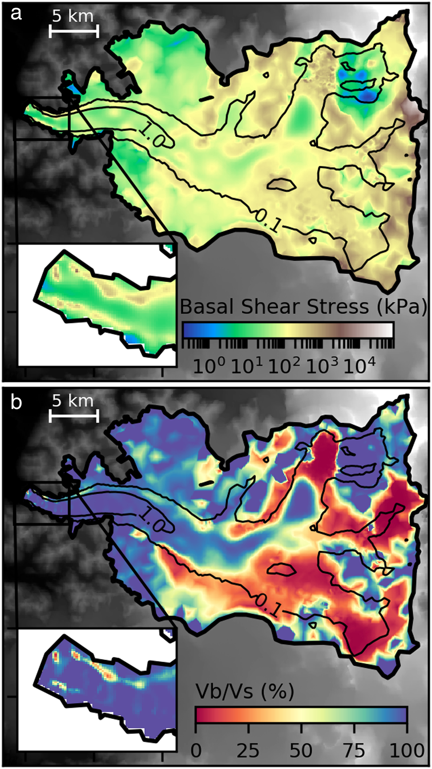
Fig. 4. (a) Basal shear stress and (b) Surface/basal velocities ratio (%). Black contour lines correspond to observed surface velocities contours (0.1 and 1.0 km a−1).
Future prognostic simulations directly start from these 100-year relaxations.
3.3. Present state of the glacier and committed mass loss
Once the initialization step has been performed, we run the model forward in time using a  $\dot b$ function in order to simulate the present state of the glacier and to constrain the response of the glacier to the long-term diffusion of the currently observed thinning. We run the model over 100 years with the same configuration and boundary conditions using as spin up the centennial relaxation period (Section 3.2.2). Importantly, the first time step of the modelling corresponds to the glacier response to the forcing estimated from observations and represent the period 2000–12. Afterwards, the simulation corresponds to the glacier response if the conditions remain fixed over 100 years. This condition represents the committed mass loss, which provides the minimum dynamical contribution of the glacier to sea-level rise in the absence of future changes in the climate or the boundary conditions (e.g. $\dot b$ function, basal friction, glacier limits, front position,…) for the next century (Price and others, Reference Price, Payne, Howat and Smith2011).
4. RESULTS
4.1. Model initialization
4.1.1. Basal friction estimation
We perform the optimizing procedure described in Section 3.2, and obtain that the optimal regularization parameter is λ = 109. The flow pattern of simulated surface velocities (Fig. 3b) is in good agreement with the observations (Fig. 3a). The map and histogram of the relative errors are shown in Figures 3c, d. The error percentage is low in the central and fastest portion of the stream with values below 10%. Errors are lower than 30% in more than 54% of the glacier area. Overall, we note a small positive bias where modelled velocities are larger than the observations. In particular, the error exceeds 100% for 13% of the area (dark green in Fig. 3c). This corresponds to mountainous areas with steep slopes and seracs where observed velocities are low (<0.1 km a−1). In these areas, the model gives deformational velocities that exceed the observed values. These values cannot be improved by the inverse method, which only affects the basal sliding component. The RMS error is 104 m a−1. This is twice larger than the reported observed velocities uncertainty of ±52 m a−1 (Mouginot and Rignot, Reference Mouginot and Rignot2015). However, this value is acceptable taking into account that part of the error is due to uncertainties in other model variables (e.g. topography, thermal state,…) that are not controlled by the inverse method. We consider that the model shows a good performance in reproducing the fast flow dynamics covering most of the glacier catchment area.
We find small basal shear stresses (below 25 kPa) in most of the fast flow areas near the glacier front and in the central portion of the stream (Fig. 4a). Consequently, the ratio between the slip velocity and the surface velocity, u b/u s, is above 0.9 over the glacier tongue where velocities exceed 1 km a−1 (Fig. 4b). Near the glacier front (insets in Figs 3, 4) the slip ratio is close to 1, indicating that surface velocities are good approximations of depth-average velocities. In this area, we also observe narrow bands of higher friction, with basal shear stresses between 50 and 500 kPa, parallel to the lateral boundaries. We suggest that this could be required by the model to compensate the free slip condition imposed at the lateral boundaries. In the steep zones where we find large relative velocity errors, the inverse method produces large basal shear stresses (>200 kPa) and the sliding velocity is nearly zero showing that the error cannot be reduced by controlling the friction only. In the upper reaches of the glacier with slow flow, the deformation should dominate. Nevertheless, the inverse method is not able to reproduce this behaviour due to the range of velocities below the mean error (<20 m a−1) and the only five layers used.
4.1.2. $\dot b$ estimation

With  $\dot b_{\rm s} $, $\dot b_{\rm k} $ and $\dot b_{{\rm k}1300} $ at the end of the relaxation the mean thickness change calculated as Δvolume/surface increase to >108, >76 and >42 m, which is much higher than the criterion threshold <10 m (Figs 5a, b). If we look at the surface elevation change, the surface increases by more than 100 m in most of the fast flowing parts, leading to velocities higher than observed and increased ice flux (see Figs 6a, b). This suggests that for these scenarios, the accumulation is too high above the ELA to be accommodated by the flow dynamics. As a consequence, we dismiss these scenarios ( $\dot b_{\rm s} $, $\dot b_{\rm k} $ and $\dot b_{{\rm k1300}} $) and try others for which the accumulation is reduced above the ELA.
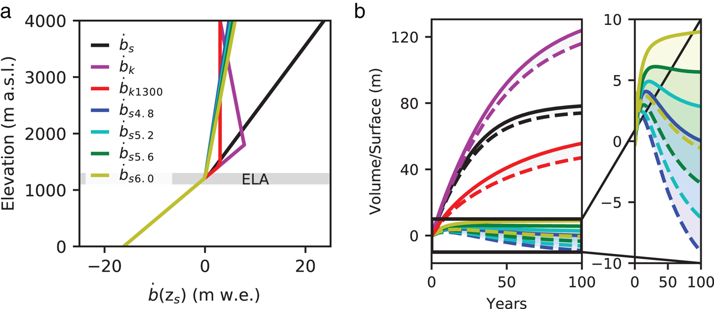
Fig. 5. (a)  $\dot b$ functions used to force the ice-flow model: $\dot b_{\rm s} $ function (black) from Schaefer and others (Reference Schaefer, Machguth, Falvey and Casassa2013), $\dot b_{\rm k} $ function (magenta) from Koppes and others (Reference Koppes, Conway, Rasmussen and Chernos2011), $\dot b_{{\rm k}1300} $ function (red) from Koppes and others (Reference Koppes, Conway, Rasmussen and Chernos2011) but modified to get an accumulation maximum at 1300 m a.s.l., $\dot b_{{\rm s}4.8} $ (in blue), $\dot b_{{\rm s}5.2} $ (cyan), $\dot b_{{\rm s}5.5} $ (green) and $\dot b_{{\rm s}6.0} $ (in yellow) functions are modified from Schaefer and others (Reference Schaefer, Machguth, Falvey and Casassa2013) with the indexes corresponding to the maximum surface mass balance at 4000 m a.s.l. (b) Relaxation volume changes results expressed in volume/surface, average over the entire glacier, for the different scenarios (same colours legend than a)). Continuous lines correspond to Δz s/Δt|AA and the discontinuous lines correspond to Δz s/Δt|SS.
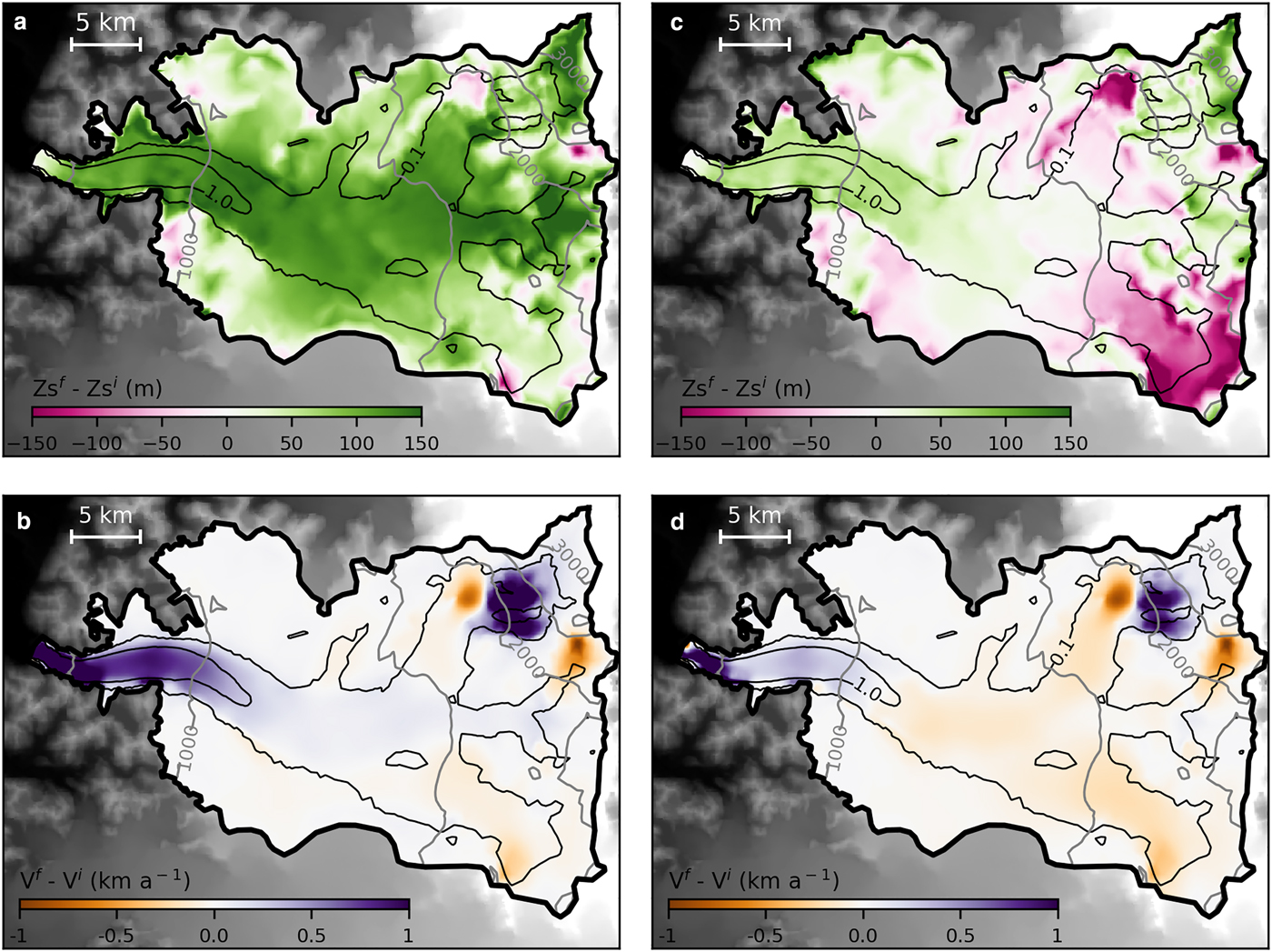
Fig. 6. (a) Total change in surface elevation (z s) after 100 years of relaxation for mass-balance scenario  $\dot b_{{\rm s}_{{\rm AA}}} $. (b) Surface velocity change after 100 years of relaxation for mass-balance scenario $\dot b_{{\rm s}_{{\rm AA}}} $. (c) Same as (a) but for scenario $\dot b_{{\rm s6}{\rm. 0}_{{\rm AA}}} $. (d) Same as (b) but for scenario $\dot b_{{\rm s6}{\rm. 0}_{{\rm AA}}} $. Gray contour lines correspond to z s contours every 500 m and black contour lines correspond to observed surface velocities contours (0.1 and 1.0 km a−1). The super-script f means final, at the end of relaxation and i means initial.
Among all the tested  $\dot b(z_{\rm s} )$ functions the four mass-balance scenarios $\dot b_{{\rm S4}{\rm. 8}} $, $\dot b_{{\rm S5}{\rm. 2}} $, $\dot b_{{\rm S5}{\rm. 6}} $ and $\dot b_{{\rm S6}{\rm. 0}} $ comply with the criterion threshold at the end of the relaxation (Figs 5a, b). We consider that after 100 years these four scenarios reach the equilibrium because mean thickness change between two-time steps (30 days) is below 0.07 m a−1, much smaller than the observed mean surface elevation change, 1.10 and 1.30 m a−1. With the scenarios $\dot b_{\rm s} $, $\dot b_{\rm k} $ and $\dot b_{{\rm k13}00} $ the volume is still increasing after 100 years but the mean surface change has largely exceeded the 10 m threshold. As the selected scenarios are at their equilibrium if we run the model further in time their increase will be very small and they will continue to be close to 10 m. In contrary, the $\dot b_{\rm s} $, $\dot b_{\rm k} $ and $\dot b_{{\rm k1300}} $ scenarios will continue to further exceed the threshold. These $\dot b$ functions correspond thus to the most realistic scenarios which agree with the dynamics and observed surface elevation rate of change. Hereafter, we refer to them as the selected scenarios.
The scenario  $\dot b_{_{{\rm S6}{\rm. 0\_AA}}} $ shows an acceptable variation of surface elevation. The surface elevation increases by more than 100 m only in a small zone in the highest part of the glacier (above 2500 m a.s.l.) and subsides by up to 140 in the south-east and within two small zones of elevated surface slopes (Fig. 6c). The surface elevation changes resulting from the other selected scenarios exhibit similar patterns (not shown). These differences are likely due to the simplified elevation-dependence chosen for the $\dot b$ variants. Surface velocity changes are usually <100 m a−1 in the upper part of the glacier, except in mountainous zones with steep slopes, seracs and discontinuous ice leading to large changes during the relaxation. The ice is shallow in these areas so we do not expect that these changes will strongly affect the flux downglacier. There is also an area with velocity changes up to nearly 1 km a−1 few kilometres upstream. As it can be seen in Figure 3a, there is a sharp discontinuity in the observed surface velocities in this area. We suspect that this discontinuity comes from the mosaicking and is not a real feature. While the model is forced by these observations during the basal friction inversion, the relaxation insures a continuity of the ice flux and thus smoothes this sharp transition. Just at the front, the velocities are very sensitive to the topography, and there is a slight decrease of the velocities during the relaxation.
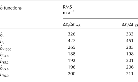
The simulated surface velocities that represent the study period forced by the selected  $\dot b$ function present the same distribution than the observed surface velocities, even though the simulated differ to the observed ones with an RMS below 211 m a−1 (see Table 2 and Fig. 7 that present the results for the scenario $\dot b_{{\rm S6}{\rm. 0\_AA}} $). Although this RMS is significant, our results are close to observations considering the uncertainties and limitations explained previously.
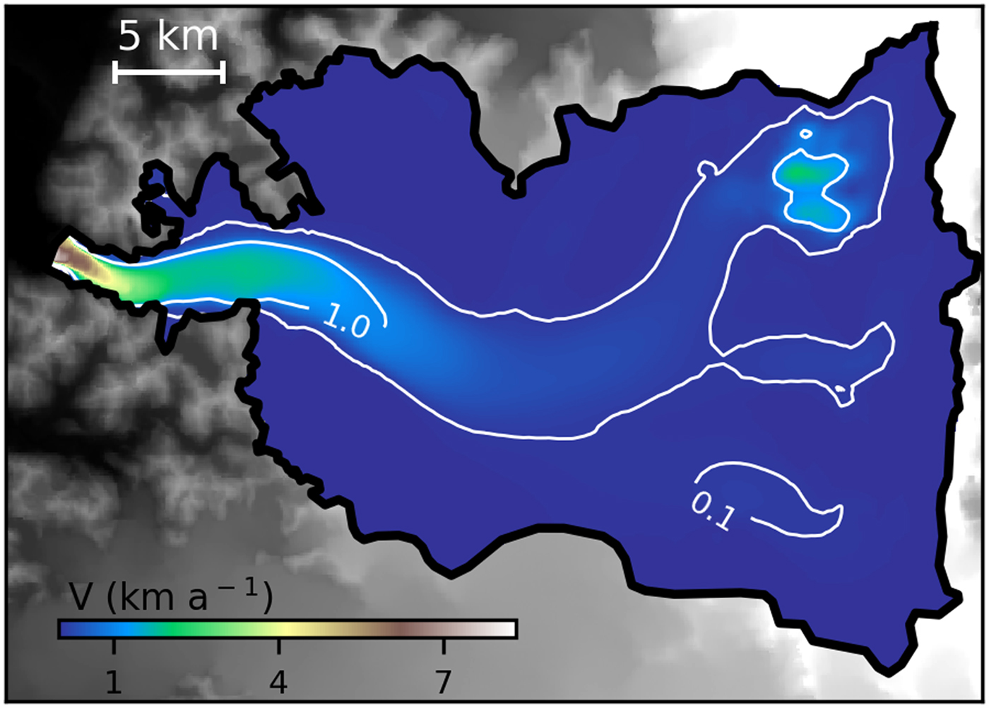
Fig. 7. Velocity after 100 years of relaxation, for scenario  $\dot b_{{\rm s6}{\rm. 0}_{{\rm AA}}} $. White contour lines correspond to simulated surface velocities contours (1000 and 100 m a−1).
Table 2. RMS between simulated and observed surface velocities from different surface mass balance ( $\dot b$) forcing
4.2. Present state of the glacier
The present state of the glacier is represented by the first time step of the prognostic simulation as explained in Section 3.3. The surface mass balance over the entire glacier is  $\dot B$ = 0.08 ± 0.06 Gt a−1, averaged over the four selected scenarios (the error is the Std dev. between the four estimates). The ice discharge estimated from the surface velocity observations and ice thickness is −0.92 Gt a−1. The model velocities were slightly larger than the observations at the beginning of the relaxation, resulting in a flux 10% larger at −1.03 Gt a−1. To accommodate the ice flux coming from upstream, this value decreases during the relaxation and, using the selected scenarios, we have $\dot D$ = −0.83 ± 0.08 Gt a−1.
The computed glacier-wide average volume change that represents the study period is −0.81 ± 0.08 km3 a−1. This is close to the value estimated from DEMs (Δz s/Δt|AA = −0.80 ± 0.06 km3 a−1 and Δz s/Δt|SS = −0.92 ± 0.07 km3 a−1 of ice), showing that our simulations capture most of the thinning pattern.
The comparison between the distribution of the simulated surface-elevation changes that represent the actual state of the glacier (Figs 8a–c) and the surface elevation changes estimated by geodetic techniques shows a good agreement. However, a lower simulated thinning compared with the observations appears at the front of the glacier, which may be related to an incorrect bedrock representation at the front in our model, to large ablation values at several locations caused by local specific processes (dust, bedrock protuberances), or to uncertainties in the surface elevation changes estimated with the geodetic techniques. Also, there are some bi-polar features in the elevation change (Fig. 8b). These features are in zones of a steep slope where the model is not capable of representing the flux and the surface change.

Fig. 8. (a) Observed rate of elevation change from ASTER DEMs. (b) Simulated rate of elevation change that represents the present state of the glacier (2000–12), for scenario  $\dot b_{{\rm s6}{\rm. 0}_{{\rm AA}}} $. (c) Comparison of the rate of elevation change for scenario $\dot b_{{\rm s6}{\rm. 0}_{{\rm AA}}} $ with the observed values using two space-borne geodetic methods (AA and SS).
4.3. Committed mass-loss results
We now run the model over 100 years forced with the four selected  $\dot b$ functions and assuming the same configuration and boundary conditions. Assuming both AA and SS surface elevation changes leads to eight different initial conditions for the estimation of the committed mass loss. The simulated and observed velocities along a flowline (Fig. 9a) generally show a similar pattern. Yet, simulated values near the glacier front are somewhat lower right from the start and decrease further with time. Ice thickness changes along a flowline (Fig. 9b) show a decrease in time, with a maximum decrease at 23.6 km inland, corresponding to an initial elevation of 1206 m a.s.l.
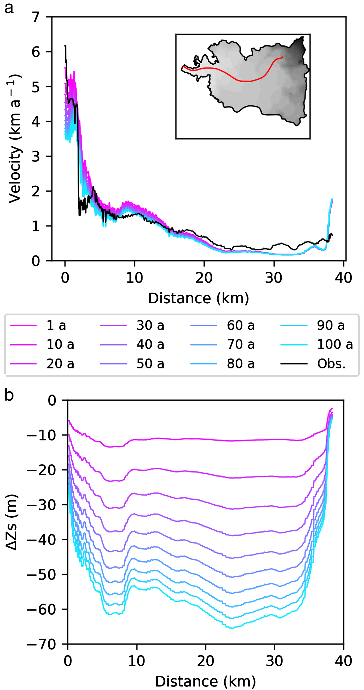
Fig. 9. (a) Velocities along a flowline (located in red in the inset) every 10 years of a 100 years long simulation compared with observed velocities (in black) for scenario  $\dot b_{{\rm s6}{\rm. 0}_{{\rm AA}}} $. (b) Change in elevation along this flowline every 10 years for scenario $\dot b_{{\rm s6}{\rm. 0}_{{\rm AA}}} $.
The committed mass loss due to the long-term diffusion of the currently observed thinning under constant forcing is equal to −33.7 ± 3.1 Gt (0.093 ± 0.008 mm SLE) after 100 years of simulations (Figs 10a–c). This corresponds to an annual loss rate of −0.34 ± 0.03 Gt a−1 being close to half the value (−0.78 ± 0.06 Gt a−1) as reported by Willis and others (Reference Willis, Melkonian, Pritchard and Rivera2012). The uncertainty is quantified using the dispersion between the eight simulations. This result corresponds to the minimum dynamical contribution of the glacier to sea-level rise in the absence of future changes during the next century.

Fig. 10. Results of the prognostic 100 years simulation for the four selected scenarios and eight initial conditions. Temporal variations of the (a) ice volume, (b) volume loss (c) mass balance ( $\dot M$), (c) ice discharge ( $\dot D$) and surface mass balance ( $\dot B$).
Because the forcing is constant in time during this experiment, the initial imbalance decreases with time as the model should tend to a steady state. The most important adjustment is in the ice discharge ( $\dot D$), which decreases as a result of both thinning and decrease of the velocity at the glacier front. While we do not take into account the surface elevation feedback for the surface mass balance, land terminated margins retreat as a response to the ablation, leading to a reduction of the glaciated area and an increase of the total mass balance $\dot B$.
5. DISCUSSION
Our ice flow model and satellite observations allow us to constrain the surface mass balance over SRG. Our best estimate of the glacier-wide surface mass balance ( $\dot B$) is slightly positive during 2000–12 at 0.08 ± 0.06 Gt a−1 (0.12 m a−1 w. eq.), which is much lower than in previous studies (Table 3). Since our results are in agreement with ice dynamics, we expect our $\dot B$ values to be better constrained than in previous studies based on atmospheric models forced by reanalysis with poor calibration in the accumulation zone. However, we are aware that there are uncertainties in the data used in this study. To support higher accumulation, the ice dynamics should be able to export more ice from the accumulation area. We have shown that basal sliding accounts for most of the observed surface velocities in larges areas. The ice flux can then reliably be estimated from the product of the surface velocity with the ice thickness. Because ice is flowing relatively fast, the surface velocities are relatively accurate, so that fluxes higher than what we estimate could be explained only by a low biased ice thickness. Using the same thickness and surface velocity datasets, Gourlet and others (Reference Gourlet, Rignot, Rivera and Casassa2016) estimated the ice flux crossing a gate at an altitude close to the ELA to be 1.49 km3 a−1. Using a gate in a similar location we obtain 1.31 km3 a−1. For each simulation, we can estimate the uniform thickness bias at the fluxgate that would be required to compensate the accumulation flux using the same surface velocity observations. For the selected scenarios, the ice thickness should be decreased by 50–74 m. Our accumulation estimates might, therefore, be biased towards lower values. On the contrary, to accommodate the accumulation from the scenario $\dot b_{\rm s} $, the ice thickness should be increased by 282 m. Gourlet and others (Reference Gourlet, Rignot, Rivera and Casassa2016) reported thickness errors up to 64 m on the plateau and up to 114 m in narrow valleys. While we cannot exclude that our results could be explained by low biased ice thicknesses, the relatively shallow thickness of SRG is consistent with bathymetry measurements and is given as a robust feature of the gravimetry inversion (Gourlet and others, Reference Gourlet, Rignot, Rivera and Casassa2016).
Table 3. San Rafael glacier-wide average surface mass balance ( $\dot B$) from different sources and periods, assuming ice density of 910 kg m−3

The range of surface areas from the different studies is 13 km2 with a maximum influence of 0.02 Gt a−1 on the B.
Regarding the  $\dot B$ distribution, all the selected $\dot b$ functions have much lower accumulation than the $\dot b_{\rm s} $ function from Schaefer and others (Reference Schaefer, Machguth, Falvey and Casassa2013) and Koppes and others (Reference Koppes, Conway, Rasmussen and Chernos2011). Our maximum accumulation at 4000 m a.s.l. is 5.4 ± 0.6 m w.e. a−1 while the maximum accumulation predicted by Schaefer and others (Reference Schaefer, Machguth, Falvey and Casassa2013) is 23.7 m w.e. a−1. We also find lower accumulation than Koppes and others (Reference Koppes, Conway, Rasmussen and Chernos2011) in the elevation range 1000–1400 m a.s.l. where most of the glacier area is (see Fig. 2b). However, due to our simplified spatial distribution of the surface mass balance, our results do not accurately represent the distribution of surface elevation changes, and they are only an example of likely $\dot b$ function among many other possibilities. Our selected scenarios do not consider that precipitation could decrease above a certain elevation which can explain why, in the model, the surface elevation increased above 2500 m a.s.l (Fig. 6c). We do not take into account either the north-south gradient in precipitation (Garreaud and others, Reference Garreaud, Lopez, Minvielle and Rojas2013) or the effect of blowing snow. Vimeux and others (Reference Vimeux2008) pointed out the importance of wind transport and erosion at Mont San Valentin. The mass loss in the south-east zone of the glacier (Fig. 6c) is compatible with regional patterns in accumulation induced by a precipitation gradient or by snow redistribution by the wind. However, a more detailed representation of surface mass-balance distribution must consider atmospheric variables and this type of modelling is beyond the scope of this study.
The selected  $\dot b$ functions allow us to check that changes in accumulation just above the ELA significantly affect glacier-wide $\dot B$ because the SRG is very flat and a large fraction of the glacier area lies around the ELA. Special attention is needed in this zone where data availability is poor (d1, d2 and d6 from Table 1) and the only direct measurement over 1 year is d6 from CECs and DGA (2012). Conversely, accumulation at even higher elevations has only a limited impact on the final $\dot B$ because only 10% of the glacier surface is located above 2000 m a.s.l. This also suggests that only small variations in the ELA may have a large impact on the final $\dot B$ and on the resulting ice dynamics.
The ice discharge resulting from the ice flow model is consistent with the results from Koppes and others (Reference Koppes, Conway, Rasmussen and Chernos2011), however, it is below the estimation from Willis and others (Reference Willis, Melkonian, Pritchard and Rivera2012) and Schaefer and others (Reference Schaefer, Machguth, Falvey and Casassa2013), see Table 4. During this period (2000–12) the observed glacier retreat was low, therefore the ice discharge and calving flux are comparable (<0.1 Gt a−1 of difference). On one hand, Schaefer and others (Reference Schaefer, Machguth, Falvey and Casassa2013) estimated the calving flux as the difference between the total mass balance and  $\dot B$. Since the $\dot B$ is very high in their study, they deduced very high calving flux values. On the other hand, Willis and others (Reference Willis, Melkonian, Pritchard and Rivera2012) computed the ice discharge from mean front velocity as 5.29 km a−1 using images collected 7-day apart on 28 March and 4 April 2007. The mean front velocity from our model is 3.83 km a−1 which is very similar to the average given by Mouginot and Rignot (Reference Mouginot and Rignot2015). The difference with the Willis and others (Reference Willis, Melkonian, Pritchard and Rivera2012) estimate is mainly a result of higher velocities at the lateral margins of the glacier at the front. We have more confidence in the velocity data used in this study because the uncertainty is smaller (52 m a−1) than the uncertainty given by Willis and others (Reference Willis, Melkonian, Pritchard and Rivera2012) (422 m a−1). However, the disagreement confirms that our simulated and observed cross-section area close to the front are likely too small compared with Willis and others (Reference Willis, Melkonian, Pritchard and Rivera2012) data. Our ice-discharge results highly depend on the bedrock uncertainty, whereas other components ( $\dot B$) should be less impacted because ice-flux changes at the front hardly propagate to the accumulation zone. Moreover, the first consequences of a higher ice discharge would be a smaller or null thickening in the lower part of the glacier after the relaxation, which would lead to a better agreement between the simulations and the geodetic results (reduction of the green area in the lower part of the glacier in Fig. 6c). This potential improvement of surface elevation changes close to the front would also be visible in Figure 8b where we currently observe a small disagreement between simulated and geodetic results below 300 m a.s.l.
Table 4. Ice-discharge ( $\dot D$) estimations, assuming ice density of 910 kg m−3

SRG is largely in disequilibrium, as demonstrated by the mass loss of the glacier during the last decade, which is mainly driven by a large ice discharge while the surface mass balance is just slightly positive. As a result of this disequilibrium, the glacier will continue to lose mass over the next 100 years even without any further changes in climate and boundary conditions. The resulting committed mass loss after one century will be −33.7 ± 3.1 Gt (−0.34 ± 0.03 Gt a−1). The committed mass balance is twice lower than the already observed wastage (see Table 5) because recent ice flow was still largely more important than the positive contribution from the  $\dot B$. However, the ice discharge will decrease with deceleration and thinning in the lower ablation area. Present rates are not sustained into the future and can therefore not be extrapolated. The committed mass-balance result is significant since it corresponds to the minimal contribution of SRG to sea level rise (SLR) over the next century and because it should be considered that the SRG represents 18% of the NPI surface.
Table 5. Sea-level contribution from earlier studies and committed mass loss from this study, assuming ice density of 910 kg m−3

A further analysis of the ice flow dynamic variations related to the glacier front location is now planned in order to estimate the influence of front geometry and front depth on the ice discharge of SRG.
Our results show that this new methodology is appropriate to independently constrain surface mass balance and ice discharge from fast-moving glaciers where ice dynamics are significant. There are many glaciers with these characteristics in Patagonia and other parts of the world such as north America and northern Europe where this methodology can improve knowledge of glacier behaviour. We recommend this method when reliable surface velocity and ice thickness data are available. Another point to be considered is that the method computes the ice discharge corresponding to a fixed front and not the calving flux. Therefore, it is only applicable during periods of time where the glacier front is stable.
6. CONCLUSION
The ice flow model Elmer/Ice was applied to reproduce the main characteristics of the ice flow dynamics of SRG. The ice dynamic model initialization demonstrated that a very low basal shear stress (<25 kPa) is inferred along the mainstream and that most of the surface velocity is due to basal sliding in the lowest part of the glacier and close to the front. After initialization, the model was used to assess the glacier-wide  $\dot B$ giving consistent modelled velocities with the observed ice velocities over the period 2000–12. This $\dot B$ is slightly positive, 0.08 ± 0.06 Gt a−1 (0.12 m w.eq. a−1), and significantly lower than in previous estimations. The modelled ice discharge is −0.83 ± 0.08 Gt a−1. Therefore, the glacier mass loss during this period resulted from an ice discharge larger than the slightly positive glacier-wide surface mass balance. In response to this state of imbalance, SRG is committed to lose ice in the coming decades and the minimum dynamical contribution of the glacier to SLR in the absence of future changes during the next century is −33.7 ± 3.1 Gt (0.093 ± 0.008 mm SLE).
Our study demonstrates that a well-calibrated ice flow model can provide an independent constrain on the poorly known surface mass balance of a large glacier such as San Rafael. The methodology developed in this study can be used on other glaciers in Patagonia where ice dynamics and discharge play an important role in the total mass balance.
7. AUTHOR CONTRIBUTION STATEMENT
GCB performed all calculations and wrote most of the paper, FGC and VF co-wrote the paper, ID and EB estimated the geodetic surface elevation changes, EB and GC contributed to the analysis and reviewed the paper, ER and JM contributed with their results and advice.
ACKNOWLEDGEMENT
This work was supported by the Chilean National Commission of Scientific and Technological Research CONICYT through a doctoral scholarship (Becas Chile) and was partly funded by the Agence Nationale de la Recherche through contract ANR-14-CE01-0001-01 (ASUMA). We thank Marius Schaefer for providing his surface mass- balance results and advice, the Unidad de Glaciología y Nieves DGA (Dirección General de Aguas) for providing data and Natalia Jiménez for her contribution as a reviewer. All model simulations presented in this paper were performed using the Froggy platform of the CIMENT infra- structure (https://ciment.ujf-grenoble.fr), supported by the Rhône-Alpes region (GRANT CPER07_13 CIRA), the OSUG@2020 labex (reference ANR10 LABX56) and the Equip@Meso project (reference ANR-10-EQPX-29-01) of the programme Investissements d'Avenir supervised by the Agence Nationale pour la Recherche. EB and ID acknowledge support from the French Space Agency (CNES).
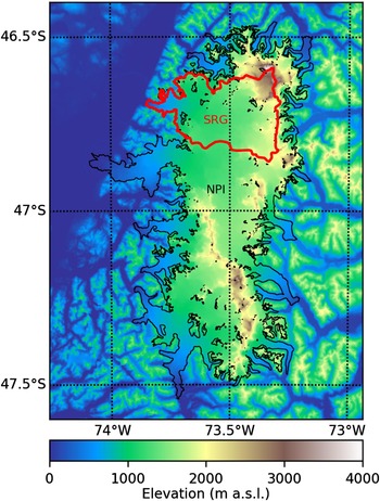
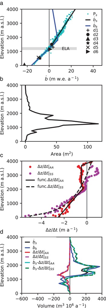

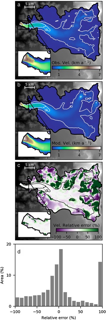


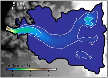

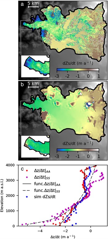
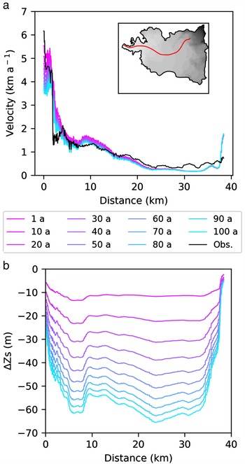
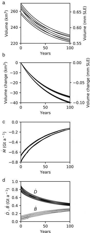


 Open access