


1 Introduction
In educational and psychological testing, pure power tests and pure speed tests aim to measure examinees’ effective abilities and effective speeds (Meijer & Sotaridona, Reference Meijer and Sotaridona2006; van der Linden, Reference van der Linden2007), respectively, under ideal testing environments. However, for the convenience of test administration, time constraints are typically imposed on the tests, resulting in what is known as time-limit tests. The degree to which the time limit of a test affects the performance of examinees is referred to as test speededness. This manifests when examinees, within the time limit, are unable to devote sufficient consideration or effort toward the end of the test (Bejar, Reference Bejar1985). Van der Linden (Reference van der Linden2011) argued that test speededness was the cumulative outcome of the interaction among the cognitive speed of the examinee, the workload of the items, and the test’s time limit. Various definitions of test speededness exist, but they all share a common aspect: Test speededness can inadvertently affect the test scores when the time limit influences the examinee’s performance, even though speed is not a core aspect of the construct that the test seeks to measure (Evans & Reilly, Reference Evans and Reilly1972; Schnipke & Scrams, Reference Schnipke and Scrams1997; Shao et al., Reference Shao, Li and Cheng2016). Such instances of speededness can induce a decrease in response accuracy, lead to missing responses (Goegebeur et al., Reference Goegebeur, De Boeck and Molenberghs2010), bias the item and ability estimates (Oshima, Reference Oshima1994), and potentially compromise the validity of the test scores by distorting or diminishing the correlation between test scores and other interested variables. This ultimately impacts the interpretation and use of test scores in decision-making processes.
Due to the necessity of time limits, it is almost impossible to entirely eliminate test speededness. Consequently, it is essential to identify response patterns affected by speededness to maintain the reliability and validity of tests. More specifically, it becomes critical to pinpoint the locations and magnitudes of test speededness at the individual level. Over several decades, various approaches have been developed to measuring and detecting test speededness, and they can be broadly classified into three categories. The first category is non-model-based approaches, such as rules of thumb and descriptive statistics, which provide basic guidelines and analytic techniques for identifying and assessing speededness. However, these methods have limitations in capturing individual differences in test speededness. To overcome this issue, the second approach known as model-based methods is proposed (e.g., Lu & Sireci, Reference Lu and Sireci2007; Schnipke & Scrams, Reference Schnipke and Scrams1997; Wise & Kong, Reference Wise and Kong2005). One such method is the hybrid modeling framework proposed by Yamamoto (Reference Yamamoto1995). This framework assumes different models before and after the speeded point, with the same speeded location for examinees (i.e., speededness homogeneity). Boughton and Yamamoto (Reference Boughton, Yamamoto, von Davier and Carstensen2007) extended this approach to the hybrid Rasch model, allowing for different speeded locations among examinees (i.e., speededness heterogeneity). Another model-based method is the two-class mixture Rasch model proposed by Bolt et al. (Reference Bolt, Cohen and Wollack2002). This model assumes a single switch point, beyond which examinees engage in rapid guessing behavior. Wang and Xu (Reference Wang and Xu2015) proposed a mixture hierarchical model to distinguish solution behavior from rapid guessing behavior based on responses and RTs, which allows to consider multiple switch points for each examinee. However, these models assumed that the probabilities of correct response after the switch points are fixed or suddenly decrease. More flexible models are needed to model the gradual switch among test-taking behaviors. Wollack and Cohen (Reference Wollack and Cohen2004) addressed this by introducing a gradual change model, where the probabilities of correct responses decline gradually after the switch point.
The third category involves detecting aberrant patterns of responses and/or RTs at individual level. Person-fit indices based on responses (e.g., Meijer & Sijtsma, Reference Meijer and Sijtsma2001) and/or RTs (Marianti et al., Reference Marianti, Fox, Marianna, Veldkamp and Tijmstra2014; van der Linden & van Krimpen-Stoop, Reference van der Linden and van Krimpen-Stoop2003) are introduced. Key to this approach is that regular behavior should be adequately fitted by a psychometric model, otherwise, it will induce false detection rate due to blurred classifications of normal and aberrant behaviors. Another popular method for detecting test speededness is the cumulative sum (CUSUM) (e.g., Armstrong & Shi, Reference Armstrong and Shi2009; Egberink et al., Reference Egberink, Meijer, Veldkamp, Schakel and Smid2010; Meijer, Reference Meijer2002; Tendeiro & Meijer, Reference Tendeiro and Meijer2012; van Krimpen-Stoop & Meijer, Reference van Krimpen-Stoop and Meijer2001). However, the CUSUM procedures have higher power only when the underlying statistical model before and after the change point are known. Change point analysis (CPA) is another approach used to detect test speededness (Sinharay, Reference Sinharay2017). Shao et al. (Reference Shao, Li and Cheng2016) implemented a CPA based on the likelihood ratio test for detecting test speededness using responses only, thereby pinpointing the locations where examinees begin to speed up. Cheng and Shao (Reference Cheng and Shao2022) extended this method, focusing solely on RTs, and utilized both likelihood ratio test and Wald test to detect test speedness. Sinharay (Reference Sinharay2016) introduced three statistics based on CPA using only responses. Subsequently, Yu and Cheng (Reference Yu and Cheng2020) conducted a comprehensive comparison between these three change-point analysis methods and twelve CUSUM methods based solely on responses. However, the above methods primarily consider either response data or RT data, lacking integration of both types of data. Even though several studies focus on responses and RTs to detect aberrancy, they are either limited to identifying cheating behavior from item preknowledge (Demirkaya, Reference Demirkaya2022; Demirkaya et al., Reference Demirkaya, Bezirhan and Zhang2023; Sinharay & Johnson, Reference Sinharay and Johnson2020) or unable to differentiate between specific types of aberrancies (Gorney et al., Reference Gorney, Sinharay and Liu2024). Recently, Lu et al. (Reference Lu, Wang, Zhang and Wang2024) proposed a real-time two-stage detection procedure to detect rapid guessing and cheating behaviors, in which Stage I identifies the aberrant RTs and then Stage II determines the type of aberrant behavior. This approach is optimal for immediate real-time monitoring and swift change detection in computer-based testing.
In contrast, likelihood ratio and Wald tests are more appropriate for post-hoc analysis on existing datasets. They involve testing a single hypothesis between two models, that is, with and without the specific change point, at a time. Specifically, null hypothesis assumes no change point (regarded as one model), and alternative hypothesis assumes a change point at a specific item location (regarded as the other model). These two methods determine whether to reject the null hypothesis based on the ratio between these two models.
In this article, we aim to provide a more effective CPA method compared to the likelihood ratio and Wald tests. The proposed CPA approaches based on Schwarz information criterion (SIC) (abbreviated as SIC-CPA) rely on the idea of model selection in statistics. SIC is preferred over other information criteria such as Akaike information criterion because it introduces a stronger penalty for model complexity, leading to more parsimonious models. This is particularly beneficial for detecting change points in noisy data, where overly complex models might capture random variations instead of true changes. Additionally, SIC has strong asymptotic properties (Chen et al., Reference Chen, Gupta and Gupta2000), ensuring that as the sample size increases, it is more likely to select the true model, thereby offering a robust and reliable framework in detecting structural changes within data.
The principle of the SIC-CPA method is as follows: it fits models to all possible change point locations, calculates the SIC value for each item location, and then the location with the smallest SIC is selected as the most possible change point. This comprehensiveness of the SIC-CPA method ensures identifying true change points more accurately. Moreover, the SIC-CPA method is computationally straightforward, thereby enhancing the computational efficiency of change point detection. More importantly, for test speededness detection with just one change point, the proposed SIC-CPA approaches take the model complexity into account when making change point decision, penalizing the model based on the number of parameters. In contrast, the likelihood ratio and Wald tests depend solely on the model fit without directly considering its complexity. Consequently, in data with subtle variations, the likelihood ratio and Wald tests might falsely pinpoint change points, leading to higher Type-I errors. In such cases, the proposed SIC-CPA approach tends to favor models without a change point, reducing the Type-I errors but possibly increasing Type-II errors. However, if the change point has a significant effect and substantially improves the model fit, the SIC-CPA approach can efficiently detect it, thereby reducing Type-II errors. Furthermore, given that the SIC-CPA approach introduces penalties for model complexity, it is more resistant to random fluctuations in the data, preventing these fluctuations from being mistaken for actual change points. All three approaches are implemented conditional on the available item parameter values, which are needed to evaluate model fit and to obtain the person parameter estimates used in the test statistics. In simulation studies, item parameters are either fixed at their true values or estimated through calibration to reflect applied testing scenarios.
In the context of aberrant behavior detection, the mixture approach often integrates both responses and RTs to differentiate between normal and aberrant behaviors. Such joint mixture models can be estimated using either Bayesian or frequentist strategies, and the computational burden depends on model specifications, estimation algorithms, and whether item parameters are treated as known. In contrast, the main advantage of the SIC-CPA method lies in its relatively simple detection-oriented and lightweight feature: when item parameters are treated as known, change points can be identified via SIC-based model comparison without needing to estimate the additional latent parameters typically involved in joint mixture models (e.g., class membership and/or person-by-item latent indicators indexing normal versus aberrant behavior). Importantly, both the SIC-CPA approach and joint mixture models typically involve estimating examinees’ ability and speed parameters. The key difference is that joint mixture models additionally model latent behavioral structure along with all model parameters simultaneously, which typically requires more complex model specification and estimation and, in some cases, involve high-dimensional data matrices (e.g., test-taking indicators at the person-by-item level). Besides, the mixture model usually requires that both response data and RT data exhibit aberrancies on the same set of items. If aberrant RTs seem normal while response data remains aberrant, the mixture model may fail to accurately identify the aberrant behavior. This is because the assumption of the mixture model, which expects aberrancies to occur in both dimensions at once, is violated in such cases. In contrast, the SIC method is capable of accurately identifying speeded behavior even when there is significant overlap between the aberrant and normal RT distributions, as long as there is a clear difference in the response data (see simulation study III for detailed analysis).
The structure of this article is as follows. First, we introduce three CPA approaches based on SIC, which focus on response data only, RT data only, and the combination of both, respectively. Second, the critical value and significance level of SIC-CPA method are given to determine whether test speededness occurs at the specific item location. Third, we conduct simulation studies to evaluate the effectiveness of the proposed SIC-CPA method in detecting test speededness. Fourth, a real data set is employed to show the application of the proposed SIC-CPA method. Finally, we conclude by discussing the strengths and limitations of this article and outline potential future research directions.
2 Method
2.1 Schwarz information criterion to detect change points
Information criteria have been extensively utilized in model selection for change point problems (Chen & Gupta, Reference Chen and Gupta1997; Yao, Reference Yao1988). SIC is a well-established method for detecting change points, and Chen and Gupta (Reference Chen and Gupta1997) showed that it is a highly effective method for detecting change points and is marginally superior to likelihood ratio procedures and Bayesian methods.
SIC is a statistical method for model selection that was first proposed by Schwarz (Reference Schwarz1978). It is more commonly known as the Bayesian information criterion (BIC) and reflects a trade-off between model fit and complexity, which is typically determined by the number of parameters.
Specifically, SICFootnote 1 is mathematically equivalent to BIC and is calculated as

where
$L\left(\widehat{\theta}\right)$
 is the maximum likelihood,
$p\times \log (n)$
is the maximum likelihood,
$p\times \log (n)$
 is called as the penalty parameter,
$p$
is called as the penalty parameter,
$p$
 is the number of parameters, and
$n$
is the number of parameters, and
$n$
 is the sample size. In change point detection, SIC is used to identify the optimal model that fits the data with the fewest number of change points.
2.2 CPA based on SIC for item responses
Throughout Section 2.2, we treat item parameters as given; this is a prerequisite for computing the likelihood and the SIC values, and the setting in which item parameters are unknown is studied in simulation study V. Given a test length of
$J$
 items to be answered by the
$i$
items to be answered by the
$i$
 th examinee, it is assumed that the
$i$
th examinee, it is assumed that the
$i$
 th examinee will answer the
$j$
th examinee will answer the
$j$
 th item with latent ability
${\theta}_{i,j}$
th item with latent ability
${\theta}_{i,j}$
 , where
$j=1,2,\dots, J$
, where
$j=1,2,\dots, J$
 . Therefore, the following hypothesis testing is considered. The null hypothesis is

against the alternative hypothesis

This alternative hypothesis assumes that change point occurs between item
$k$
 and
$k+1$
and
$k+1$
 .
.
As an illustration, the traditional two parameter logistic model (2PLM; Birnbaum, Reference Birnbaum, Lord and Novick1968) is used as the item response theory (IRT) model, that is,

In Eq. (4),
${y}_{ij}$
 represents the response of the
$i$
represents the response of the
$i$
 th examinee answering the
$j$
th examinee answering the
$j$
 th item, where
$i=1,\dots, N$
th item, where
$i=1,\dots, N$
 and
$j=1,\dots J$
and
$j=1,\dots J$
 . The correct response probability is expressed as
${P}_j\left({\theta}_i\right)$
. The correct response probability is expressed as
${P}_j\left({\theta}_i\right)$
 , and the corresponding incorrect response probability is
${Q}_j\left({\theta}_i\right)=1-{P}_j\left({\theta}_i\right).{a}_j$
, and the corresponding incorrect response probability is
${Q}_j\left({\theta}_i\right)=1-{P}_j\left({\theta}_i\right).{a}_j$
 is the discrimination parameter of the
$j$
is the discrimination parameter of the
$j$
 th item, and
${b}_j$
th item, and
${b}_j$
 is the difficulty parameter of the
$j$
is the difficulty parameter of the
$j$
 th item.
${\theta}_i$
th item.
${\theta}_i$
 denotes the latent ability of the
$i$
denotes the latent ability of the
$i$
 th examinee.
Therefore, under
${H}_0^{\theta }$
 , the maximum likelihood function based on the 2PL model is

where
${\boldsymbol{y}}_i$
 denotes the vector of item responses for the
$i$
denotes the vector of item responses for the
$i$
 th examinee, that is,
${\boldsymbol{y}}_i={\left({y}_{i1},{y}_{i2},\dots, {y}_{iJ}\right)}^{\prime }$
th examinee, that is,
${\boldsymbol{y}}_i={\left({y}_{i1},{y}_{i2},\dots, {y}_{iJ}\right)}^{\prime }$
 .
${\widehat{\theta}}_i$
.
${\widehat{\theta}}_i$
 is the maximum likelihood estimate (MLE) of the latent ability obtained from the responses based on all items of the test. Therefore, the SIC (Chen & Gupta, Reference Chen and Gupta1997; Schwarz, Reference Schwarz1978) under
${H}_0^{\theta }$
is the maximum likelihood estimate (MLE) of the latent ability obtained from the responses based on all items of the test. Therefore, the SIC (Chen & Gupta, Reference Chen and Gupta1997; Schwarz, Reference Schwarz1978) under
${H}_0^{\theta }$
 , that is,
${\mathrm{SIC}}_{\theta }(J)$
, that is,
${\mathrm{SIC}}_{\theta }(J)$
 , can be expressed as

where
${P}_j{\left(\hat{\theta}\right)}_i)$
 and
${Q}_j\left({\widehat{\theta}}_i\right)$
and
${Q}_j\left({\widehat{\theta}}_i\right)$
 are the values of
${P}_j\left(\theta \right)$
are the values of
${P}_j\left(\theta \right)$
 and
${Q}_j\left(\theta \right)$
and
${Q}_j\left(\theta \right)$
 by plugging in
${\widehat{\theta}}_i$
by plugging in
${\widehat{\theta}}_i$
 , respectively.
Here, the item parameters are available, and only one latent ability parameter is needed to be estimated for the examinee
$i$
 under the null hypothesis. Therefore, the number of parameters included in the penalty term is 1 (i.e.,
$p=1$
under the null hypothesis. Therefore, the number of parameters included in the penalty term is 1 (i.e.,
$p=1$
 ), and the number of observations included in the penalty term is
$J$
), and the number of observations included in the penalty term is
$J$
 (i.e.,
$n=J$
(i.e.,
$n=J$
 ). Note that when item parameters are unknown, the penalty term should include both item and person parameters. As a result, the effective penalty becomes substantially larger, which may make the criterion more conservative in selecting a change point model.
Under
${H}_1^{\theta }$
 , the corresponding maximum likelihood function can be obtained as

where
${\widehat{\theta}}_i$
 and
${\widehat{\theta}}_i^{\prime }$
and
${\widehat{\theta}}_i^{\prime }$
 are the MLEs of the latent ability obtained from the responses based on the
$k$
are the MLEs of the latent ability obtained from the responses based on the
$k$
 and
$J-k$
and
$J-k$
 items in the test, respectively. Therefore, the
$\mathrm{SIC}$
items in the test, respectively. Therefore, the
$\mathrm{SIC}$
 under
${H}_1^{\theta }$
under
${H}_1^{\theta }$
 , that is,
${\mathrm{SIC}}_{\theta }(k)$
, that is,
${\mathrm{SIC}}_{\theta }(k)$
 , for
$k=2,\dots, J-1$
, for
$k=2,\dots, J-1$
 , can be expressed as

where the number of parameters included in the penalty term is 2 (i.e.,
$p=2$
 ). According to the minimum information criterion principle,
${H}_0$
). According to the minimum information criterion principle,
${H}_0$
 is rejected if

and the estimated change point position denoted by
$\widehat{k}$
 such that

Remark 1. Although the SIC method can be applied to detect change points at any position in theory, it is suggested to be used when the ability parameters are accurately estimated. In other words, there needs to be a sufficient number of items available both before and after the change point.
Remark 2. The SIC method can be extended to identify multiple change points by performing a series of hypothesis testing for a given response sequence. The process involves the following steps:
Step 1: The null hypothesis, as defined by Eq. (2), is tested against the alternative hypothesis given by Eq. (3) to determine if there is a change point. If
${H}_0^{\theta }$
 is not rejected, then no change point is present, and the process stops. If
${H}_0^{\theta }$
is not rejected, then no change point is present, and the process stops. If
${H}_0^{\theta }$
 is rejected, then the estimated position of the change point, denoted by
$\widehat{k}$
is rejected, then the estimated position of the change point, denoted by
$\widehat{k}$
 , is determined by Eq. (10), where
$\widehat{k}$
, is determined by Eq. (10), where
$\widehat{k}$
 is the location of the single change point at this stage. The process then moves to Step 2.
Step 2: The SIC method is used to test the two subsequences before and after the change point detected by Step 1 separately for a change.
Step 3: Repeat the process until no further subsequences have change points.
Step 4: The collection of change point locations found by Steps 1–3 is denoted by
$\left({\widehat{k}}_1,{\widehat{k}}_2,\dots, {\widehat{k}}_M\right)$
 , and the estimated total number of change points is
$M$
, and the estimated total number of change points is
$M$
 . Note that the calculation of SIC-CPA incorporates a penalty for model complexity, effectively preventing the selection of overly complex models with multiple change points.
Although SIC-CPA method can detect multiple change points, this study mainly focuses on detecting test speededness, and in common scenarios, examinees exhibit a single change point at the end of the test due to factors such as test fatigue, motivation less, test disengagement behavior, etc. Further investigation of the SIC-CPA method for detecting two change points can be found in simulation study IV.
2.3 CPA based on SIC for item response times
Similarly, considering a test with
$J$
 items, examinee
$i$
items, examinee
$i$
 answers item
$j$
answers item
$j$
 with a speed parameter of
${\tau}_{i,j}$
with a speed parameter of
${\tau}_{i,j}$
 , where
$j=1,2,\dots, J$
, where
$j=1,2,\dots, J$
 . The hypothesis testing problem is considered as follows: The null hypothesis is

and the alternative hypothesis is

In this study, the traditional log-normal model (van der Linden, Reference van der Linden2006) is used to fit the RT data, that is,

where
${\alpha}_j$
 and
${\beta}_j$
and
${\beta}_j$
 are time dispersion and time intensity parameters for item
$j$
are time dispersion and time intensity parameters for item
$j$
 , respectively.
${\tau}_i$
, respectively.
${\tau}_i$
 is the speed parameter of examinee
$i$
is the speed parameter of examinee
$i$
 . Therefore, under
${H}_0^{\tau }$
. Therefore, under
${H}_0^{\tau }$
 , the maximum likelihood function of observing a RT pattern
${\boldsymbol{t}}_i$
, the maximum likelihood function of observing a RT pattern
${\boldsymbol{t}}_i$
 for the
$i$
for the
$i$
 th examinee can be obtained as

where
${\boldsymbol{t}}_i={\left({t}_{i1},{t}_{i2},\dots, {t}_{iJ}\right)}^{\prime }$
 is a RT pattern that captures the RTs of examinee
$i$
is a RT pattern that captures the RTs of examinee
$i$
 answering all items of the test. Therefore, the
$\mathrm{SIC}$
answering all items of the test. Therefore, the
$\mathrm{SIC}$
 under
${H}_0^{\tau }$
under
${H}_0^{\tau }$
 , that is,
${\mathrm{SIC}}_{\tau }(J)$
, that is,
${\mathrm{SIC}}_{\tau }(J)$
 , is
, is

Here, we assume that the item parameters are known, and only one latent speed parameter is needed to be estimated for examinee
$i$
 under the null hypothesis. Therefore, the number of parameters included in the penalty term is 1 (i.e.,
$p=1$
under the null hypothesis. Therefore, the number of parameters included in the penalty term is 1 (i.e.,
$p=1$
 ), and the number of observations is
$J$
), and the number of observations is
$J$
 (i.e.,
$J$
(i.e.,
$J$
 is number of all RT observations for examinee
$i$
is number of all RT observations for examinee
$i$
 ).
).
Under
${H}_1^{\tau }$
 , the corresponding maximum likelihood function is

where
${\widehat{\tau}}_i$
 and
${\hat{\tau}}_i^{\prime }$
and
${\hat{\tau}}_i^{\prime }$
 are the MLEs of the speed parameter obtained by calculating the
$m$
are the MLEs of the speed parameter obtained by calculating the
$m$
 and
$J-m$
and
$J-m$
 RTs, respectively. Therefore, the SIC under
${H}_1^{\tau },{\mathrm{SIC}}_{\tau }(m)$
RTs, respectively. Therefore, the SIC under
${H}_1^{\tau },{\mathrm{SIC}}_{\tau }(m)$
 , for
$m=2,\dots, J-1$
, for
$m=2,\dots, J-1$
 , is obtained as

where the number of parameters included in the penalty term is 2 (i.e.,
$p=2$
 ). Based on the minimum information criterion principle, we reject
${H}_0^{\tau }$
). Based on the minimum information criterion principle, we reject
${H}_0^{\tau }$
 if
if

and the estimated change point position denoted by
$\widehat{m}$
 such that

2.4 CPA based on SIC for item responses and response times
A modified SIC method is proposed to detect test speededness by combining both response and RT data. The key to the hypothesis testing is to examine whether the ability and speed parameters change simultaneously during the responding process. We consider the following hypothesis testing problem: The null hypothesis is

and the alternative hypothesis is

Here, van der Linden’s (Reference van der Linden2006) joint model for responses and RTs is considered. Therefore, under
${H}_0$
 , the maximum likelihood function of observing response and RT pattern
$\left({\boldsymbol{y}}_{\boldsymbol{i}},{\boldsymbol{t}}_{\boldsymbol{i}}\right)$
, the maximum likelihood function of observing response and RT pattern
$\left({\boldsymbol{y}}_{\boldsymbol{i}},{\boldsymbol{t}}_{\boldsymbol{i}}\right)$
 for examinee
$i$
for examinee
$i$
 is
is

where
${\boldsymbol{y}}_{\boldsymbol{i}}=\left({y}_{i1},{y}_{i2},\dots, {y}_{ij},\dots {y}_{iJ}\right)$
 is the response pattern of examinee
$i$
is the response pattern of examinee
$i$
 and
${\boldsymbol{t}}_i={\left({t}_{i1},{t}_{i2},\dots, {t}_{iJ}\right)}^{\prime }$
and
${\boldsymbol{t}}_i={\left({t}_{i1},{t}_{i2},\dots, {t}_{iJ}\right)}^{\prime }$
 is the RT pattern of examinee
$i$
is the RT pattern of examinee
$i$
 . Therefore, the
$\mathrm{SIC}$
. Therefore, the
$\mathrm{SIC}$
 under
${H}_0$
under
${H}_0$
 , that is,
${\mathrm{SIC}}_{\theta, \tau }(J)$
, that is,
${\mathrm{SIC}}_{\theta, \tau }(J)$
 , is
, is

Under
${H}_1$
 , the corresponding maximum likelihood function is

where
${\widehat{\theta}}_i$
 and
${\widehat{\tau}}_i$
and
${\widehat{\tau}}_i$
 are the MLEs of the ability and speed parameters obtained from the first
$r$
are the MLEs of the ability and speed parameters obtained from the first
$r$
 responses and RTs, respectively,
${\hat{\theta}}_i^{\prime }$
responses and RTs, respectively,
${\hat{\theta}}_i^{\prime }$
 and
${\hat{\tau}}_i^{\prime }$
and
${\hat{\tau}}_i^{\prime }$
 are the corresponding MLEs obtained from the remaining
$J-r$
are the corresponding MLEs obtained from the remaining
$J-r$
 responses and RTs, respectively. Therefore, the SIC under
${H}_1,{\mathrm{SIC}}_{\theta, \tau }(r)$
responses and RTs, respectively. Therefore, the SIC under
${H}_1,{\mathrm{SIC}}_{\theta, \tau }(r)$
 , for
$r=2,\dots, J-1$
, for
$r=2,\dots, J-1$
 , is obtained as

where the number of parameters included in the penalty term is 4 (i.e.,
$p=4$
 ). Based on the minimum information criterion principle, we reject
${H}_0$
). Based on the minimum information criterion principle, we reject
${H}_0$
 if
if

and the estimated change point position denoted by
$\widehat{r}$
 such that

2.5 Critical value and significance level of CPA based SIC method
According to Gupta and Chen (Reference Gupta and Chen1996), when the difference between SICs is small, it may be difficult to determine whether the change point actually exists or is simply caused by data fluctuation. In our study, the fluctuation of responses and/or RTs may induce subtle differences in SICs, which may result in examinees without change points being incorrectly identified as speeded (i.e., exhibiting changes in ability and/or speed). For example, as verified based solely on responses in our simulation study I, among the examinees without change points, 75% of the
$\mathrm{SI}{\mathrm{C}}_{\theta }(J)-{\min}_{2\le k\le J-1}\kern0.1em \mathrm{SI}{\mathrm{C}}_{\theta }(k)$
 is less than critical value, which results in an extremely high Type-I error. To solve this problem, Gupta and Chen (Reference Gupta and Chen1996) introduced the significance level
$\alpha$
is less than critical value, which results in an extremely high Type-I error. To solve this problem, Gupta and Chen (Reference Gupta and Chen1996) introduced the significance level
$\alpha$
 and its associated critical value
${c}_{\alpha }$
and its associated critical value
${c}_{\alpha }$
 , where
${c}_{\alpha}\ge 0$
, where
${c}_{\alpha}\ge 0$
 . Therefore, we accept
${H}_0$
. Therefore, we accept
${H}_0$
 if
if

where

Unfortunately, as the (joint) distribution of our models (i.e., 2PL model, log-normal RT model, or van der Linden’s (Reference van der Linden2006) joint response and RT model) is not normal, it is not feasible to obtain a closed form of the exact critical value
${c}_{\alpha }$
 . Usually, permutation (Shao et al., Reference Shao, Li and Cheng2016), bootstrap, and simulation (Armstrong & Shi, Reference Armstrong and Shi2009; Cheng & Shao, Reference Cheng and Shao2022) methods are commonly used to determine the critical values in detecting aberrancy. However, permutation and bootstrap methods are computationally expensive. Therefore, in this study, empirical critical values were used via Monte Carlo simulations following the procedure outlined by Worsley (Reference Worsley1979) and further adopted in Cheng and Shao (Reference Cheng and Shao2022). Specifically, we generated 10,000 data under the null hypothesis—each dataset representing individual responses, RTs, or a combination of both, depending on the data type used in the SIC-CPA method. For each dataset, we computed the SIC values using estimated ability and/or speed parameters, while treating the item parameters as known. As a result, these 10,000 datasets consist solely of regular data, without any aberrancies. Note that the resulting critical values are determined by the simulation settings, such as test length, item parameters, and the distribution of person parameters, rather than by the proportion of speeded examinees. For the significance levels of 0.05, 0.01, and 0.001 in a one-sided test, the 500th, 100th, and 10th largest values were selected as critical values, respectively. For each test length condition, 1000 replicated processes were performed, and the average critical value of 1000 times was used as the final critical value for each SIC-CPA approach.
3 Simulation studies
Six simulation studies were carried out to investigate the performance of the proposed SIC-CPA approaches, which employed distinct data, including responses, RTs, and a combination of response and RT data, respectively. Specifically, simulation study I compared the proposed SIC-CPA method with Shao et al.’s (Reference Shao, Li and Cheng2016) method, based solely on response data. In simulation study II, we compared the proposed SIC-CPA method and Cheng and Shao’s (Reference Cheng and Shao2022) method, based solely on RT data. Simulation study III compared the performance of the proposed three SIC-CPA methods; in this case, the data were generated from the modified gradual change joint model for responses and RTs. To manipulate test speededness, examinees with one change point were considered in simulation studies I, II, and III. Simulation study IV was conducted to evaluate the performance of the SIC-CPA method based on RTs with two change points, simultaneously considering the warm-up effect and test speededness. Simulation study V includes an item parameter estimation stage and considers two cases: (1) non-iterative calibration-detection procedure and (2) iterative detect–clean–recalibrate procedure. Under each case, we compare the SIC-CPA with the likelihood ratio and Wald tests. In addition, simulation study VI was conducted to evaluate the performance of the SIC-CPA, likelihood ratio test, and Wald methods when there are no speeded responses and/or response times (RTs) in the data. Due to page limit, simulation study VI can be found in the Supplementary Material. Each simulation condition was conducted 100 replications.
3.1 Data generation
Concerning the generation models for regular and speeded responses and/or RTs, as claimed in Gorney and Wollack’s (Reference Gorney and Wollack2022) paper, “All response accuracy (RA) models are formulated as mixture extensions of the IRT model. All RT models are formulated as mixture extensions of the lognormal RT model developed by van der Linden (Reference van der Linden2006).” The unique difference between these generation models (for example, van der Linden & van Krimpen-Stoop, Reference van der Linden and van Krimpen-Stoop2003; Wang & Xu, Reference Wang and Xu2015; Wollack & Cohen, Reference Wollack and Cohen2004) is the degree of change in the responses/RTs or ability/speed parameter, and thus they can be classified as abrupt and gradual change models. We adopted the gradual change model proposed by Suh et al., (Reference Suh, Cho and Wollack2012) for responses, along with its extensions for RTs developed by Cheng and Shao (Reference Cheng and Shao2022), as well as our modified gradual change joint model for responses and RTs to generate simulation data. These models were chosen because they offer a more realistic representation and can capture the complexity of real data. Furthermore, employing more sophisticated models for data generation allows for a more comprehensive evaluation of the robustness and flexibility of the proposed approaches (Cheng & Shao, Reference Cheng and Shao2022; Luecht & Ackerman, Reference Luecht and Ackerman2018).
Next, we introduce a modified gradual change joint model for responses and RTs:


where


and
$p\left({y}_{ij}=1\mid {\theta}_i,{a}_j,{b}_j\right)$
 follows the 2PL model in Eq. (4),
${\eta}_i$
follows the 2PL model in Eq. (4),
${\eta}_i$
 (where
$0<{\eta}_i<1$
(where
$0<{\eta}_i<1$
 ) is the stage of the test that test speededness occurs on examinee
$i$
) is the stage of the test that test speededness occurs on examinee
$i$
 , and
${\eta}_i\times J$
, and
${\eta}_i\times J$
 is the location of change point. For instance, if
${\eta}_i=0.7$
is the location of change point. For instance, if
${\eta}_i=0.7$
 , it indicates that test speededness occurs at 70% of a test, and if there are 50 items in the test (i.e.,
$J=50$
, it indicates that test speededness occurs at 70% of a test, and if there are 50 items in the test (i.e.,
$J=50$
 ), the change point would be item 35. The parameter
${\lambda}_i$
), the change point would be item 35. The parameter
${\lambda}_i$
 (where
${\lambda}_i\ge 0$
(where
${\lambda}_i\ge 0$
 ) is the speededness rate which controls how fast the correct response probability decreases as the test proceeds beyond
${\eta}_i$
) is the speededness rate which controls how fast the correct response probability decreases as the test proceeds beyond
${\eta}_i$
 , at the same time,
${\lambda}_i$
, at the same time,
${\lambda}_i$
 determines the rate at which less time is spent on items after
${\eta}_i$
determines the rate at which less time is spent on items after
${\eta}_i$
 . When
${\lambda}_i$
. When
${\lambda}_i$
 increases, it leads to faster declines of
${P}_j^{\ast}\left({\theta}_i\right)$
increases, it leads to faster declines of
${P}_j^{\ast}\left({\theta}_i\right)$
 and
$\log \left({t}_{ij}\right)$
and
$\log \left({t}_{ij}\right)$
 due to test speededness. For example, take two examinees with different
$\lambda$
due to test speededness. For example, take two examinees with different
$\lambda$
 and the same
$\eta$
and the same
$\eta$
 as an example, when
$\frac{j}{J}>\eta$
as an example, when
$\frac{j}{J}>\eta$
 we have
$\min {\left(1,\left[1-\left(\frac{j}{J}-\eta \right)\right]\right)}^{\lambda_i}={\left[1-\left(\frac{j}{J}-\eta \right)\right]}^{\lambda_i}$
we have
$\min {\left(1,\left[1-\left(\frac{j}{J}-\eta \right)\right]\right)}^{\lambda_i}={\left[1-\left(\frac{j}{J}-\eta \right)\right]}^{\lambda_i}$
 , and if
${\lambda}_1>{\lambda}_2$
, and if
${\lambda}_1>{\lambda}_2$
 , then
${\left[1-\left(\frac{j}{J}-{\eta}_i\right)\right]}^{\lambda_1}<{\left[1-\left(\frac{j}{J}-{\eta}_i\right)\right]}^{\lambda_2}$
, then
${\left[1-\left(\frac{j}{J}-{\eta}_i\right)\right]}^{\lambda_1}<{\left[1-\left(\frac{j}{J}-{\eta}_i\right)\right]}^{\lambda_2}$
 , which means that
${P}_j^{\ast}\left({\theta}_1\right)<{P}_j^{\ast}\left({\theta}_2\right)$
, which means that
${P}_j^{\ast}\left({\theta}_1\right)<{P}_j^{\ast}\left({\theta}_2\right)$
 and
$\log \left({t}_{1j}\right)<\log \left({t}_{2j}\right)$
and
$\log \left({t}_{1j}\right)<\log \left({t}_{2j}\right)$
 . This modified gradual change joint model is reduced to van der Linden’s (Reference van der Linden2006) hierarchical response and RT model when
${\eta}_i=0$
. This modified gradual change joint model is reduced to van der Linden’s (Reference van der Linden2006) hierarchical response and RT model when
${\eta}_i=0$
 and
${\lambda}_i=0$
and
${\lambda}_i=0$
 , which means the test speededness does not happen, and hence the responses and RTs are from the regular behavior. Note that Suh et al.’s (Reference Suh, Cho and Wollack2012) gradual change model for responses and the extended gradual model for RTs used in Cheng and Shao (Reference Cheng and Shao2022) are both special cases of this modified gradual change model for responses and RTs.
Table 1 displays the manipulated factors and their varied levels used in all four simulation studies. Here, 500 and 1,000 examinees were considered, and the proportions of speeded examinees were 10% and 30%, respectively. Three test lengths, 20 (short test), 50 (moderate test) and 80 (long test), were considered, as used in Zhu et al. (Reference Zhu, Jiao, Gao and Meng2023). Following the data generation scheme in Shao et al. (Reference Shao, Li and Cheng2016) and Cheng and Shao (Reference Cheng and Shao2022),
$\eta$
 was simulated from Beta distribution, and we set the median of
$\eta$
was simulated from Beta distribution, and we set the median of
$\eta$
 to 0.5, 0.6, 0.7, 0.8 and 0.9, and the variance of
$\eta$
to 0.5, 0.6, 0.7, 0.8 and 0.9, and the variance of
$\eta$
 was set to 0.001, 0.01, and 0.04. Because the detection results are consistent across sample sizes, we only show the simulation results for 500 examinees. In general, 90 (i.e., 3 (test lengths)
$\times$
was set to 0.001, 0.01, and 0.04. Because the detection results are consistent across sample sizes, we only show the simulation results for 500 examinees. In general, 90 (i.e., 3 (test lengths)
$\times$
 2 (speededness proportions)
$\times$
2 (speededness proportions)
$\times$
 5 (median of
$\eta$
5 (median of
$\eta$
 )
$\times$
)
$\times$
 3 (variance of
$\eta$
3 (variance of
$\eta$
 )) baseline simulation conditions were conducted. We implemented the SIC-CPA, Shao et al. (Reference Shao, Li and Cheng2016), and Cheng and Shao (Reference Cheng and Shao2022) approaches using the R programming language (R Core Team, 2022) on a computer equipped with Intel(R) Core(TM) i7-7700HQ CPU at 2.80 GHz, 8 GB RAM. Supplementary Table S1 shows the average values of critical values and the standard deviations (SD) for the SIC-CPA, likelihood ratio test, and Wald statistics across 1,000 replicated processes in simulation studies I, II, and III at the significant level of 0.01.
Fixed factors/parameters in four simulation studies.

Table 1 Long description
The table consists of two columns titled Factor and Values.
* Row 1: Factor is Number of examinees. Value is 500.
* Row 2: Factor is Test length. Values are 20, 50, 80.
* Row 3: Factor is Proportion of examinees with test speededness. Values are 10 percent, 30 percent.
* Row 4: Factor is the Greek letter eta. Values are listed as Median (0.5, 0.6, 0.7, 0.8, 0.9) times Variance (0.001, 0.01, 0.04).
3.2 Evaluation criteria
We evaluate the performance of the proposed approaches from three aspects. First, concerning the detection of speeded examinees, we focus on the correct classification rate (CCR), power and Type I errors. CCR is the ratio of correctly classified examinees (including normal and speeded examinees) to the total number of examinees, power is the proportion of correctly identified speeded examinees among all identified speeded examinees, and Type I error rate is the proportion of normal examinees incorrectly classified as speeded examinees. Second, we assess the performance of the proposed method in pinpointing change points. We use “lag,” which is equal to estimated location of change point minus true location of change point, to show the recoveries of estimating change points. Because “positive lags” and “negative lags” offset each other, the “average absolute lag” (AL_mean) and its standard deviation (AL_SD) are used to compare the performance of different methods in locating change points. Third, the computational time is given to show the efficiency of the different approaches.
3.3 Simulation study I
This simulation study evaluates the performance of the proposed SIC-CPA approach based solely on the responses. Meanwhile, we compare the effectiveness of the SIC-CPA approach with Shao et al.’s (Reference Shao, Li and Cheng2016) CPA method, hereafter referred to as Shao-CPA. The speeded responses were generated from Suh et al.’s (Reference Suh, Cho and Wollack2012) gradual change model, that is, Eq. (31), and the non-speeded responses were generated from the 2PL model in Eq. (4). For the model parameters, we simulate
${a}_j\sim \log N\left(\mathrm{0,0.5}\right)$
 ,
${b}_j\sim N\left(0,1\right)$
,
${b}_j\sim N\left(0,1\right)$
 ,
${\theta}_i\sim N\left(0,1\right)$
,
${\theta}_i\sim N\left(0,1\right)$
 , and
${\lambda}_i\sim \log N\left(\mathrm{3.912,1}\right)$
, and
${\lambda}_i\sim \log N\left(\mathrm{3.912,1}\right)$
 . We sampled
${\lambda}_i$
. We sampled
${\lambda}_i$
 values from
$\log N\left(\mathrm{3.912,1}\right)$
values from
$\log N\left(\mathrm{3.912,1}\right)$
 following the previous studies (Goegebeur et al., Reference Goegebeur, De Boeck, Wollack and Cohen2008; Suh et al, Reference Suh, Cho and Wollack2012), which generated various test speededness patterns. Specifically, this choice represents a reasonable range of performance that accounts for both typical and extreme test speededness, ensuring that the model can simulate the full spectrum of examinee behaviors: the majority of examinees experience a gradual decline in performance, whereas a minority exhibits more extreme speededness near the end of the test. Note that, in Shao et al.’s (Reference Shao, Li and Cheng2016) simulation study, a permutation method was used to generate the null distribution for the Shao-CPA test statistics, with the false discovery rate set to 0.2. To ensure a fair comparison between their approach and our SIC-CPA approach, we used Monte Carlo simulations to determine the critical values for these two methods. Due to consistent trends in the SIC-CPA method with different critical values and page limit, we present the significance level of 0.01 for these two approaches.
Supplementary Tables S2–S4 present the detection results of Shao-CPA and SIC-CPA methods with test lengths of 20, 50, and 80, respectively. Both methods maintain the type I error rates around 0.01 across all conditions. For the test with 20 items (Supplementary Table S2), the performance of both methods in terms of CCR and power is similar. However, SIC-CPA performs better under high speeded examinee proportions (30%) and larger values of the median and variance of
$\eta$
 . Specifically, SIC-CPA achieves lower AL_mean and AL_SD, which indicates more accurate change point estimation. When the median of
$\eta$
. Specifically, SIC-CPA achieves lower AL_mean and AL_SD, which indicates more accurate change point estimation. When the median of
$\eta$
 is 0.8, the power of both methods drops below 0.43 when the proportion of speeded examinees is 30%. This decline can be attributed to the fact that the change point locations for speeded examinees approached the end of the test, resulting in fewer speeded responses, which in turn diminishes the performance of identifying speeded examinees and pinpointing the change points.
For the test with 50 (or 80) items in Supplementary Table S3 (or S4), as the median of
$\eta$
 increases, both CCRs and powers of these two methods decrease in most cases. When the variance of
$\eta$
increases, both CCRs and powers of these two methods decrease in most cases. When the variance of
$\eta$
 increases, indicating greater variations in change point locations, both AL_mean and AL_SD increase, indicating a decrease in change point estimation accuracy. As the proportion of speeded examinees increases, the performance of these two methods declines, and specifically, CCRs and powers decrease. Meanwhile, it becomes more difficult to accurately identify change point locations, leading to higher AL_mean and AL_SD values.
As the test length increases, Shao-CPA shows an increase in both AL_mean and AL_SD. This is because Shao-CPA struggles to accurately locate change points with longer tests, which is consistent with the findings of Shao et al. (Reference Shao, Li and Cheng2016). However, as the test length grows, the performance of detecting speeded examinees improves, resulting in consistently higher CCRs and power for both two methods. In particular, when the median of
$\eta$
 is 0.8, the power of these two approaches remains above 0.56 under the condition of 30% speeded examinees, as shown in Supplementary Table S4. Furthermore, the advantages of SIC-CPA become more evident, especially under high values of median and variance of
$\eta$
is 0.8, the power of these two approaches remains above 0.56 under the condition of 30% speeded examinees, as shown in Supplementary Table S4. Furthermore, the advantages of SIC-CPA become more evident, especially under high values of median and variance of
$\eta$
 . This suggests that SIC-CPA is more robust in handling data variability and it provides more accurate and stable estimates of change points. Therefore, SIC-CPA proves to be a more reliable and efficient approach, particularly in scenarios involving higher speeded examinee proportion and greater variability in the data.
Table 2 shows the average running time of Shao-CPA and SIC-CPA when the sample size is 500. It is evident that the SIC-CPA method operates quickly, indicating a higher computational efficiency. Note that under each simulation condition, the average running time reported in this article indicates the average time for a single replication, and the running time does not include the Monte Carlo simulations used to obtain the empirical critical value.
Average running time of Shao-CPA and SIC-CPA approaches when sample size is 500 in simulation study I.

Table 2 Long description
The table consists of three columns and four rows including the header.
Column 1: Test length.
Column 2: Shao C P A (seconds).
Column 3: S I C C P A (seconds).
Data rows:
* Row 1: Test length 20. Shao C P A is 2.5. S I C C P A is 0.9.
* Row 2: Test length 50. Shao C P A is 5.6. S I C C P A is 2.8.
* Row 3: Test length 80. Shao C P A is 8.9. S I C C P A is 5.5.
The data shows that S I C C P A consistently has a lower running time than Shao C P A across all test lengths, and both methods show a linear increase in time as test length increases.
3.4 Simulation study II
Simulation study II was conducted to assess the performance of the proposed SIC-CPA approach utilizing only RTs, and to compare its performance with Cheng and Shao’s (Reference Cheng and Shao2022) CPA method. The speeded RTs were generated from the extended gradual change model for RTs used in Cheng and Shao (Reference Cheng and Shao2022), that is, Eq. (32). For the model parameters,
${\alpha}_j\sim U\left(\mathrm{1.75,3.25}\right)$
 ,
${\beta}_j\sim U\left(\mathrm{3.6,0.11}\right)$
,
${\beta}_j\sim U\left(\mathrm{3.6,0.11}\right)$
 ,
${\tau}_i\sim N\left(\mathrm{0,0.25}\right)$
,
${\tau}_i\sim N\left(\mathrm{0,0.25}\right)$
 , and
${\lambda}_i\sim \log N\left(\mathrm{3.912,1}\right)$
, and
${\lambda}_i\sim \log N\left(\mathrm{3.912,1}\right)$
 . In addition, the time limits for the test lengths of 20, 50, and 80 were 30, 75, and 120 min, respectively. 90 simulation conditions were conducted, please see Table 1.
Due to the consistency of results obtained from both the Wald test and likelihood ratio test, aligning with the findings from Cheng and Shao (Reference Cheng and Shao2022), this simulation study only presents the results of the Wald test. Supplementary Tables S5–S7 display the detection results of SIC-CPA method and the Wald test under the significance level of 0.01. The last column in these two tables indicates the proportion of examinees who did not complete the test within the time limit, ranging from 4% to 8%. This suggests that the majority of speeded examinees can complete the test on time. Consistent with Cheng and Shao (Reference Cheng and Shao2022), this article labels examinees who did not complete the test as speeded without performing any statistical analysis.
Overall, the results of SIC-CPA and the Wald test are nearly identical, with SIC-CPA having slightly lower Type I errors. Both methods achieve high CCRs exceeding 0.9 except under the condition with 30% speeded examinee proportion and
${\eta}_{\mathrm{median}}=0.9$
 ,
${\eta}_{\mathrm{var}}=0.04$
,
${\eta}_{\mathrm{var}}=0.04$
 . However, when the proportion of speeded examinees is 30%, detection becomes more challenging because the change points are located closer to the end of the test. Under the condition of 30% speeded examinee proportion with
${\eta}_{\mathrm{median}}=0.9$
. However, when the proportion of speeded examinees is 30%, detection becomes more challenging because the change points are located closer to the end of the test. Under the condition of 30% speeded examinee proportion with
${\eta}_{\mathrm{median}}=0.9$
 ,
${\eta}_{\mathrm{var}}=0.04$
,
${\eta}_{\mathrm{var}}=0.04$
 , the power of both methods decrease substantially.
Regarding the accuracy of change point estimation, when the median of
$\eta$
 is 0.9, both AL_mean and AL_SD are relatively small, indicating precise change point estimation. As
$\eta$
is 0.9, both AL_mean and AL_SD are relatively small, indicating precise change point estimation. As
$\eta$
 variance increases, the power decreases, but the accuracy of change point estimation remains high. Furthermore, as the test length increases, the performance of recovering change points for both methods deteriorate, which is consistent with findings of simulation study I. Under the condition of 30% speeded examinee proportion with
${\eta}_{\mathrm{median}}=0.9$
variance increases, the power decreases, but the accuracy of change point estimation remains high. Furthermore, as the test length increases, the performance of recovering change points for both methods deteriorate, which is consistent with findings of simulation study I. Under the condition of 30% speeded examinee proportion with
${\eta}_{\mathrm{median}}=0.9$
 and
${\eta}_{\mathrm{var}}=0.04$
and
${\eta}_{\mathrm{var}}=0.04$
 , SIC-CPA outperforms Shao-CPA in change point estimation accuracy, showing lower values of AL_mean and AL_SD.
Table 3 shows the average running time for SIC-CPA method, Wald test, and likelihood ratio test under the test lengths of 20, 50, and 80 when sample size is 500. It is observed that both the SIC-CPA method and Wald test exhibit similar running times. In addition, SIC-CPA is more efficient than the likelihood ratio test.
Average running time of SIC-CPA approach, Wald test, and likelihood ratio test when sample size is 500 in simulation study II.

Table 3 Long description
The table consists of four columns and three data rows. The columns are labeled Test length, S I C dash C P A (seconds), Wald test (seconds), and Likelihood ratio test (seconds).
* For a test length of 20: S I C dash C P A is 0.2, Wald test is 0.3, and Likelihood ratio test is 0.6.
* For a test length of 50: S I C dash C P A is 0.5, Wald test is 0.4, and Likelihood ratio test is 1.1.
* For a test length of 80: S I C dash C P A is 0.7, Wald test is 0.5, and Likelihood ratio test is 1.9.
The data shows that the Likelihood ratio test is consistently the slowest, while S I C dash C P A and the Wald test maintain significantly lower running times as test length increases.
3.5 Simulation study III
This simulation study aims to evaluate the performance of the proposed SIC-CPA approach using responses and RTs. In addition, we compared the results with those from the other two SIC-CPA approaches that used either responses or RTs solely. The speeded responses and RTs were simulated using the modified gradual change joint model for responses and RTs (please see Eqs. (30)–(33)). Van der Linden’s (Reference van der Linden2006) hierarchical response and RT model (i.e., Eqs. (30)–(33) with
${\eta}_i=0$
 and
${\lambda}_i=0$
and
${\lambda}_i=0$
 ) was used to generate the non-speeded responses and RTs. For speeded examinee
$i$
) was used to generate the non-speeded responses and RTs. For speeded examinee
$i$
 , to ensure that the speeded response and RT data are aligned at the same change point, the same values of
${\eta}_i$
, to ensure that the speeded response and RT data are aligned at the same change point, the same values of
${\eta}_i$
 and
${\lambda}_i$
and
${\lambda}_i$
 in Eqs. (30) and (31) were used for the modified gradual change joint model for responses and RTs. The person parameters were sample from
$\left(\begin{array}{l}{\theta}_i\\ {}{\tau}_i\end{array}\right)\sim \mathrm{MVN}\left(\left(\begin{array}{c}0\\ {}0\end{array}\right),{\Sigma}_p=\left(\begin{array}{cc}1& {\sigma}_{\theta \tau}\\ {}{\sigma}_{\theta \tau}& 0.25\end{array}\right)\right)$
in Eqs. (30) and (31) were used for the modified gradual change joint model for responses and RTs. The person parameters were sample from
$\left(\begin{array}{l}{\theta}_i\\ {}{\tau}_i\end{array}\right)\sim \mathrm{MVN}\left(\left(\begin{array}{c}0\\ {}0\end{array}\right),{\Sigma}_p=\left(\begin{array}{cc}1& {\sigma}_{\theta \tau}\\ {}{\sigma}_{\theta \tau}& 0.25\end{array}\right)\right)$
 . Here, we manipulated two levels of correlation coefficients between ability and speed parameters, that is, 0.5 and 0.8, which corresponds to
${\sigma}_{\theta \tau}=0.25$
. Here, we manipulated two levels of correlation coefficients between ability and speed parameters, that is, 0.5 and 0.8, which corresponds to
${\sigma}_{\theta \tau}=0.25$
 and 0.4 respectively. The item parameters were simulated as follows:
$\left(\begin{array}{l}{b}_j\\ {}{\beta}_j\end{array}\right)\sim \mathrm{MVN}\left({\mu}_I=\left(\begin{array}{c}0\\ {}3.6\end{array}\right),{\Sigma}_I=\left(\begin{array}{cc}1& 0.15\\ {}0.15& 0.2\end{array}\right)\right)$
and 0.4 respectively. The item parameters were simulated as follows:
$\left(\begin{array}{l}{b}_j\\ {}{\beta}_j\end{array}\right)\sim \mathrm{MVN}\left({\mu}_I=\left(\begin{array}{c}0\\ {}3.6\end{array}\right),{\Sigma}_I=\left(\begin{array}{cc}1& 0.15\\ {}0.15& 0.2\end{array}\right)\right)$
 (Gorney et al., Reference Gorney, Sinharay and Liu2024),
${a}_j\sim \log N\left(\mathrm{0,0.5}\right)$
(Gorney et al., Reference Gorney, Sinharay and Liu2024),
${a}_j\sim \log N\left(\mathrm{0,0.5}\right)$
 , and
${\alpha}_j\sim U\left(\mathrm{1.75,3.25}\right)$
, and
${\alpha}_j\sim U\left(\mathrm{1.75,3.25}\right)$
 (Lu & Wang, Reference Lu and Wang2020; Lu et al., Reference Lu, Wang, Zhang and Tao2020, Reference Lu, Wang and Shi2023). Again, the time limits for tests with 20, 50, and 80 items were set at 30, 75, and 120 min, respectively. In addition, we evaluated the sensitivity of our proposed SIC-CPA approaches under four distinct scenarios. Scenarios 1–4 explored two common underlying mechanisms of test speededness (Yu & Cheng, Reference Yu and Cheng2020): gradual change model (GCM) and hybrid model (HM) with abrupt changes, respectively. Scenario 1 serves as a baseline scenario, similar to the setups used in simulations 1 and 2. Equations (34) and (35) describe the HM models for responses and RTs, respectively. Thus, Eqs. (32)–(35) constitute the joint HM model for responses and RTs. Scenarios 2 and 3 manipulated the abrupt changes in correct response probability together with gradual changes in RTs after the change points. This occurs when examinees shift to providing incorrect or random answers, leading to reduced accuracy and progressively faster responses (i.e., gradual changes in RTs) as they adapt to the new answering strategy or experience cognitive disengagement. We set
$g=0$
(Lu & Wang, Reference Lu and Wang2020; Lu et al., Reference Lu, Wang, Zhang and Tao2020, Reference Lu, Wang and Shi2023). Again, the time limits for tests with 20, 50, and 80 items were set at 30, 75, and 120 min, respectively. In addition, we evaluated the sensitivity of our proposed SIC-CPA approaches under four distinct scenarios. Scenarios 1–4 explored two common underlying mechanisms of test speededness (Yu & Cheng, Reference Yu and Cheng2020): gradual change model (GCM) and hybrid model (HM) with abrupt changes, respectively. Scenario 1 serves as a baseline scenario, similar to the setups used in simulations 1 and 2. Equations (34) and (35) describe the HM models for responses and RTs, respectively. Thus, Eqs. (32)–(35) constitute the joint HM model for responses and RTs. Scenarios 2 and 3 manipulated the abrupt changes in correct response probability together with gradual changes in RTs after the change points. This occurs when examinees shift to providing incorrect or random answers, leading to reduced accuracy and progressively faster responses (i.e., gradual changes in RTs) as they adapt to the new answering strategy or experience cognitive disengagement. We set
$g=0$
 to represent an extreme but practically relevant scenario in which examinees stop solving items due to severe time pressure or disengagement, yielding nearly uniformly incorrect answers toward the end of the test; a similar pattern was reported in Shao et al. (Reference Shao, Li and Cheng2016, see Figure 4 in their real data analysis). This setting is also reasonable for high-stakes tests with difficult end-of-test items, where accurate responses cannot be made without spending reasonable amount of time. In contrast,
$g=0.25$
to represent an extreme but practically relevant scenario in which examinees stop solving items due to severe time pressure or disengagement, yielding nearly uniformly incorrect answers toward the end of the test; a similar pattern was reported in Shao et al. (Reference Shao, Li and Cheng2016, see Figure 4 in their real data analysis). This setting is also reasonable for high-stakes tests with difficult end-of-test items, where accurate responses cannot be made without spending reasonable amount of time. In contrast,
$g=0.25$
 represents random guessing behavior (Wang & Xu, Reference Wang and Xu2015), typical in multiple-choice questions with four options. In scenario 2, we use the uniform distribution to simulate
${\lambda}_i$
represents random guessing behavior (Wang & Xu, Reference Wang and Xu2015), typical in multiple-choice questions with four options. In scenario 2, we use the uniform distribution to simulate
${\lambda}_i$
 , representing mild speededness where most examinees show gradual performance changes without extreme fluctuations. In contrast, the log-normal distribution of
$\lambda$
, representing mild speededness where most examinees show gradual performance changes without extreme fluctuations. In contrast, the log-normal distribution of
$\lambda$
 simulates heterogeneous speededness, including both gradual and stable declines in performance, as well as extreme declines, reflecting diverse real-world scenarios. Table 4 depicts data generation manners for responses and RTs under four scenarios. In total, there are 720 (i.e., 90 baseline conditions [please see Table 1]
$\times$
simulates heterogeneous speededness, including both gradual and stable declines in performance, as well as extreme declines, reflecting diverse real-world scenarios. Table 4 depicts data generation manners for responses and RTs under four scenarios. In total, there are 720 (i.e., 90 baseline conditions [please see Table 1]
$\times$
 2 (correlation coefficients)
$\times$
2 (correlation coefficients)
$\times$
 4 (scenarios)) simulation conditions. Figure 1 shows the histogram of log RTs for all person-by-item combinations for four scenarios:


Generated models and parameter settings for responses and RTs under four scenarios in simulation study III.

Table 4 Long description
The table consists of four columns and four data rows.
* Scenario 1: Generated model is G C M: Eqs. 30 to 33. Responses parameter is lambda sub i sim log N (3.912, 1). R Ts parameter is lambda sub i sim log N (3.912, 1).
* Scenario 2: Generated model is H M plus G C M: Eqs. 31 to 34. Responses parameter is g = 0. R Ts parameter is lambda sub i sim Uniform (10, 20).
* Scenario 3: Generated model is H M plus G C M: Eqs. 31 to 34. Responses parameter is g = 0.25. R Ts parameter is lambda sub i sim log N (3.912, 1).
* Scenario 4: Generated model is H M: Eqs. 32 to 35. Responses parameter is g = 0. R Ts parameter is C sub i j sim U (1 sec, 20 sec).
Histogram of log RTs for all person-by-item combinations for four scenarios. Note that the histogram of scenario 3 is identical to that of scenario 1. The “speeded” refers to all speeded RTs at person-by-item level, “unspeeded” indicates all normal RTs at person-by-item level.

Figure 1 Long description
The figure consists of three side-by-side histograms. Each panel shares a Y-axis labeled Frequency ranging from 0 to 3500 and an X-axis labeled Log response time ranging from -4 to 2. A legend in each panel identifies blue bars as speeded and red bars as unspeeded.
* Scenario 1 (Left Panel): Shows a sharp, narrow blue peak at the far left (x = -4) reaching a frequency of 3500. A separate, broad bell-shaped red distribution is centered near x = -0.5, peaking around 1750.
* Scenario 2 (Middle Panel): Displays a shorter blue peak at x = -4 reaching approximately 1750, with a small tail extending to the right. The red distribution remains a broad bell curve centered near x = -0.5.
* Scenario 4 (Right Panel): The blue distribution is shifted right and flattened, forming a low mound between x = -4 and -1. The red distribution is a broad bell curve centered near x = -0.5, overlapping significantly with the right tail of the blue distribution, creating a purple shaded area of intersection.
Tables 5 and 6, along with Supplementary Tables S8–S11, show the detection results of scenario 1 in simulation study III. Overall, compared to the SIC-CPA using only RT data, the SIC-CPA using response and RT data shows slightly higher CCRs, nearly identical power except when the median of
$\eta$
 is 0.9, and lower Type I errors. The power of the SIC-CPA using combined data is notably higher than that using only response data. Regarding the accuracy of change point location recovery, the SIC-CPA using only response data performs the worst; in most cases, the SIC-CPA using RT data performs slightly better than when using combined data. This could be attributed to the variability in discrete response data caused by test speededness, which impacts the accuracy of recovering change point locations. In particular, when the change points occur at the end of the test, as seen when the median of
$\eta$
is 0.9, and lower Type I errors. The power of the SIC-CPA using combined data is notably higher than that using only response data. Regarding the accuracy of change point location recovery, the SIC-CPA using only response data performs the worst; in most cases, the SIC-CPA using RT data performs slightly better than when using combined data. This could be attributed to the variability in discrete response data caused by test speededness, which impacts the accuracy of recovering change point locations. In particular, when the change points occur at the end of the test, as seen when the median of
$\eta$
 is 0.8 and 0.9, the AL_mean and AL_SD for SIC-CPA using RTs are smaller than those for SIC-CPA using combined data.
Results of the proposed three SIC-CPA approaches when the correlation coefficient of person parameters is 0.5 and test length is 50 for scenario 1 in simulation study III.

Table 5 Long description
The table presents results for three approaches: Y and T (responses and response times), R T (response times only), and Y (responses only).
Header Structure:
* The primary columns are C C R, Power, Type I, A L mean, A L S D, and N F percentage.
* Each primary column (except N F percentage) is subdivided into the three approaches: Y and T, R T, and Y.
* The leftmost columns define the conditions: Percentage (10 or 30), eta median (0.5 to 0.9), and eta var (0.001, 0.01, or 0.04).
Key Data Trends:
* For Percentage 10, eta var 0.001: C C R values for Y and T and R T are high (0.992 to 0.994), while Y is lower (0.917 to 0.963). Power for Y and T and R T is consistently 1.000, but drops significantly for Y as eta median increases (from 0.713 at 0.5 to 0.222 at 0.9).
* For Percentage 30, eta var 0.04: Detection performance drops substantially at eta median 0.9. Power for Y and T is 0.403, R T is 0.247, and Y is 0.112 (all marked in bold).
* Type I error rates remain stable across most conditions, generally ranging between 0.006 and 0.012.
* N F percentage (Non-convergence) ranges from approximately 7.072 to 9.420 across all scenarios.
Note: “Y&T” indicates SIC-CPA approach based on responses and RTs, “RT” indicates SIC-CPA approach based on response times, and “Y” indicates SIC-CPA approach based on responses. Boldface values indicate substantially lower detection performance than other conditions within the same scenario.
Results of the proposed three SIC-CPA approaches when the correlation coefficient of person parameters is 0.8 and test length is 50 for scenario 1 in simulation study III.

Table 6 Long description
The table presents results for three approaches: Y and T (responses and response times), R T (response times only), and Y (responses only). The data is organized by two main blocks representing different percentages (10 and 30). Within each block, rows are categorized by eta median (0.5 to 0.9) and eta variance (0.001, 0.01, and 0.04).
Key performance metrics include:
* C C R: Values for Y and T and R T are consistently high (0.935 to 0.995), while Y values are lower (0.737 to 0.961).
* Power: Y and T and R T frequently reach 1.000 in lower eta median conditions but drop significantly at eta median 0.9, especially at 0.04 variance (0.448 and 0.409 respectively). Y power is consistently lower, dropping to 0.150.
* Type I Error: Remains stable across all conditions, ranging between 0.007 and 0.012.
* A L mean and A L S D: Y and T and R T generally show lower average lengths and standard deviations compared to the Y approach.
* N F percentage: Ranges from approximately 6.5 to 8.8 percent across all scenarios.
Boldface values highlight substantially lower detection performance, primarily occurring at the eta median of 0.9 across all variance levels.
Note: “Y&T” indicates SIC-CPA approach based on responses and RTs, “RT” indicates SIC-CPA approach based on response times, and “Y” indicates SIC-CPA approach based on responses. Boldface values indicate substantially lower detection performance than other conditions within the same scenario.
When the number of items increases, the power of the SIC-CPA using only response data significantly improves. The Type I errors of both the SIC-CPA using combined data and the SIC-CPA using response data slightly increase. The detection results of the SIC-CPA using only RT data are almost unaffected by the increase in test length. In terms of detecting speeded examinees, the performance of the SIC-CPA using combined data and SIC-CPA using RT data is nearly identical. As the number of items increases, the accuracy of change point location recovery declines for the SIC-CPA using all three types of data, as evidenced by larger AL_mean and AL_SD.
In summary, compared to the SIC-CPA using only response data, the SIC-CPA using combined data and the SIC-CPA using RT data present higher CCRs and power, as well as lower AL_mean and AL_SD. The SIC-CPA using combined data and the SIC-CPA using RT data outperform the SIC-CPA using only response data in detecting speeded examinees and in recovering change point locations.
When the correlation coefficient between
$\theta$
 and
$\tau$
and
$\tau$
 is 0.8, the trends of results in terms of these evaluation criteria are almost identical to those when the correlation coefficient is 0.5. As the correlation coefficient between
$\theta$
is 0.8, the trends of results in terms of these evaluation criteria are almost identical to those when the correlation coefficient is 0.5. As the correlation coefficient between
$\theta$
 and
$\tau$
and
$\tau$
 increases, SIC-CPA using combined data shows particularly notable improvements in detecting speeded examinees, showing higher power compared with SIC-CPA using RTs.
The results of scenarios 2, 3, and 4 under different correlation coefficients between
$\theta$
 and
$\tau$
and
$\tau$
 , as well as different test lengths, are essentially consistent with the results of scenario 1. Due to the page limit, we only present the results for the correlation coefficient between
$\theta$
, as well as different test lengths, are essentially consistent with the results of scenario 1. Due to the page limit, we only present the results for the correlation coefficient between
$\theta$
 and
$\tau$
and
$\tau$
 of 0.8, for 500 examinees, across 15 conditions. The specific conditions are shown in Table 7. The detailed results can be found in Supplementary Tables S12–S20.
Simulation conditions with different values for the median and variance of
$\eta$
 in four scenarios of simulation study III.

Table 7 Long description
The table consists of three rows and 16 columns.
Row 1: Simulation condition. Columns 1 through 15 are labeled numerically from 1 to 15.
Row 2: Median of eta.
- Conditions 1 to 5: 0.5, 0.6, 0.7, 0.8, 0.9.
- Conditions 6 to 10: 0.5, 0.6, 0.7, 0.8, 0.9.
- Conditions 11 to 15: 0.5, 0.6, 0.7, 0.8, 0.9.
Row 3: Variance of eta.
- Conditions 1 to 5: 0.001 for all.
- Conditions 6 to 10: 0.01 for all.
- Conditions 11 to 15: 0.04 for all.
Figure 2 displays the power, Type I error, and AL_mean of 15 simulation conditions for four scenarios for the condition of 10% speeded examinee proportion with test length 50. In scenario 2, unlike the gradual decline correct response probability observed in scenario 1, the correct response probability of speeded responses suddenly drops to zero. This change significantly improves the performance of the SIC-CPA using response data in detecting speeded examinees and pinpointing change point locations. Furthermore, scenario 2 demonstrates that while the results using RT data alone are less satisfactory than in scenario 1, the results from using response data are superior. Moreover, combining both types of data yields better detection results than using RT data alone, with a higher power than that of using response data alone.
Power, Type I errors, and AL_mean of 15 simulation conditions for 4 scenarios in simulation study III.

Figure 2 Long description
A multi-panel figure with 3 rows and 4 columns. A legend in the top-left indicates three methods: Y and T (green line with squares), R T (blue dashed line with triangles), and Y (red line with dots).
Row 1: Power. The y-axis ranges from 0 to 1. In all scenarios, Y and T and R T maintain high power near 1.0, dropping sharply at condition 15. Method Y shows a saw-tooth pattern with lower overall power, peaking around 0.7 to 0.8.
Row 2: Type I error. The y-axis ranges from 0 to 0.02. All methods remain stable between 0.005 and 0.01. R T generally shows the highest error rate, while Y and T and Y fluctuate at slightly lower levels.
Row 3: A L mean. The y-axis ranges from 0 to 6.
- Scenario 1: Y and T and R T are flat near 1, while Y shows a saw-tooth increase between 1 and 3.
- Scenario 2: Y and T and R T show a saw-tooth pattern between 1 and 2.5, while Y is low and stable.
- Scenario 3: Y and T and R T are flat near 1, while Y shows high volatility between 3 and 6.
- Scenario 4: Y and T and Y are low and stable near 0.5, while R T is stable near 1.5.
In scenario 3, the correct response probability of speeded responses suddenly drops to 0.25. Compared to scenario 1, the performance of the SIC-CPA using response data for detecting speeded examinees and pinpointing change points diminishes. The power of the SIC-CPA using combined data is identical to those using RT data alone except for the median of
$\eta$
 is 0.9. In most conditions, the use of combined data results in lower Type I errors compared to using RT data alone. Therefore, combining response and RT data proves to be more effective than using either response or RT data alone. Furthermore, even when response data alone shows reduced performance, the inclusion of RT data allows the SIC-CPA to maintain high performance, demonstrating the robustness of the combined data approach.
Figure 1 shows that in scenario 4, the speeded RTs largely overlap with normal RTs, resulting in suboptimal detection results when using RTs alone, as expected. However, even with a high degree of overlap between speeded and normal RTs, the power of the SIC-CPA using RT data consistently exceeds 90%, with Type I errors staying below 0.012. Figure 2 illustrates that using combined data provides greater advantages in identifying speeded examinees and pinpointing change point locations. For instance, all AL_mean values detected using combined data are consistently lower than those detected using response data alone. Therefore, even when there is little distinction between normal and speeded RTs, with a clear distinction between normal and speeded response data, the SIC-CPA using combined data still effectively detects the speeded examinees and provides better accuracy in change point recovery.
Table 8 displays the average running times for the SIC-CPA using three types of data, under the test lengths of 20, 50, and 80. It is observed that the SIC-CPA using only RT data operates faster, while the running time for using combined data and response data are closely comparable.
Average running time of SIC-CPA approach when sample size is 500 in simulation study III.

Table 8 Long description
The table consists of four columns and three data rows.
Columns are labeled as follows:
* Test length
* Y and T (seconds)
* R T (seconds)
* Y (seconds)
Data rows:
* For a Test length of 20: Y and T is 1.1, R T is 0.3, and Y is 0.9.
* For a Test length of 50: Y and T is 2.9, R T is 0.5, and Y is 2.7.
* For a Test length of 80: Y and T is 6.0, R T is 0.6, and Y is 5.3.
Note: Y and T indicates S I C dash C P A approach based on responses and R Ts. R T indicates S I C dash C P A approach based on response times. Y indicates S I C dash C P A approach based on responses.
Note: “Y&T” indicates SIC-CPA approach based on responses and RTs, “RT” indicates SIC-CPA approach based on response times, and “Y” indicates SIC-CPA approach based on responses.
3.6 Simulation study IV
This simulation study was conducted to evaluate the performance of the SIC-CPA approach based on RTs to identify multiple change points. The study does not focus on aberrant behaviors occurring at isolated items, as these could lead to a large number of change points, making accurate detection more challenging. Instead, we manipulated the common aberrant test-taking behavior scenarios, that is, the warm-up effect at the very beginning of the test and the test speededness at the end of the test due to the time limit, resulting in two change points. Essentially, these two common aberrant behaviors can be seen as forms of speeding-up behavior, reflected in an increasing trend of speed parameters throughout different phases of the test. Specifically, examinees often struggle to settle at the beginning of the test, and the warm-up effect leads to longer RTs (Shao, Reference Shao2017), resulting in lower speed parameters. Afterward, they respond at a normal pace, exhibiting typical speeds. Finally, due to time pressure, they speed up toward the end of the test, which is reflected in higher speeds.
Following the simulation study designed by Zhu et al. (Reference Zhu, Jiao, Gao and Meng2023) to manipulate RTs with the warm-up effect and test speededness, we generated the RTs using the following model proposed by van der Linden and van Krimpen-Stoop (Reference van der Linden and van Krimpen-Stoop2003):

where
$L$
 captures the speed shift caused by aberrant behavior, reflecting the extent of an abrupt change in an examinee’s speed. When
$L>0$
captures the speed shift caused by aberrant behavior, reflecting the extent of an abrupt change in an examinee’s speed. When
$L>0$
 , longer RTs indicate warm-up effect, whereas when
$L<0$
, longer RTs indicate warm-up effect, whereas when
$L<0$
 , shorter RTs reflect test speededness. When
$L=0$
, shorter RTs reflect test speededness. When
$L=0$
 , the model simplifies to Eq. (1
3), representing the regular behavior. We set the first change point occurring between items 5 and 8, which means the warm-up effect is observed across items 1–4, 1–5, 1–6, and 1–7, respectively. The second change point is determined by the median and variance of
$\eta$
, the model simplifies to Eq. (1
3), representing the regular behavior. We set the first change point occurring between items 5 and 8, which means the warm-up effect is observed across items 1–4, 1–5, 1–6, and 1–7, respectively. The second change point is determined by the median and variance of
$\eta$
 , with the specific values provided in Table 1. For the RTs associated with the warm-up effect, we set
$L=1$
, with the specific values provided in Table 1. For the RTs associated with the warm-up effect, we set
$L=1$
 , and for the RTs related to test speededness,
$L=-1\;\mathrm{or}-2$
, and for the RTs related to test speededness,
$L=-1\;\mathrm{or}-2$
 . The other model parameters are consistent with those in simulation study II. Thus, 2 (speed shifts for test speededness, we denote two scenarios as
${L}_{\mathrm{speeded}}=-1$
. The other model parameters are consistent with those in simulation study II. Thus, 2 (speed shifts for test speededness, we denote two scenarios as
${L}_{\mathrm{speeded}}=-1$
 or
$-2$
or
$-2$
 )
$\times$
)
$\times$
 90 (baseline condition in Table 1) produces 180 simulation conditions.
Supplementary Tables S21–S26 show the detection results of the SIC-CPA approach based on RTs for identifying two change points in simulation study IV. Figure 3 depicts the results of simulation study IV under 10% speeded examinee proportion, including power, type I error rate, and AL_mean for each of the two change points (i.e.,
$\mathrm{Al}\_{\mathrm{mean}}_{\mathrm{warm}-\mathrm{up}}$
 ,
$\mathrm{Al}\_{\mathrm{mean}}_{\mathrm{speeded}}$
,
$\mathrm{Al}\_{\mathrm{mean}}_{\mathrm{speeded}}$
 ) as well as their AL_mean summation (i.e.,
$\mathrm{Al}\_{\mathrm{mean}}_{\mathrm{sum}}$
) as well as their AL_mean summation (i.e.,
$\mathrm{Al}\_{\mathrm{mean}}_{\mathrm{sum}}$
 ). Across all test lengths, SIC-CPA approach under
${L}_{\mathrm{speeded}}=-2$
). Across all test lengths, SIC-CPA approach under
${L}_{\mathrm{speeded}}=-2$
 consistently shows higher power than those under
${L}_{\mathrm{speeded}}=-1$
consistently shows higher power than those under
${L}_{\mathrm{speeded}}=-1$
 . When test length is 20, the power under
${L}_{\mathrm{speeded}}=-2$
. When test length is 20, the power under
${L}_{\mathrm{speeded}}=-2$
 is below 0.9, while power under
${L}_{\mathrm{speeded}}=-1$
is below 0.9, while power under
${L}_{\mathrm{speeded}}=-1$
 falls under 0.6. When
${\eta}_{\mathrm{median}}$
falls under 0.6. When
${\eta}_{\mathrm{median}}$
 is set at 0.5 or 0.9, the power is notably lower than when
${\eta}_{\mathrm{median}}$
is set at 0.5 or 0.9, the power is notably lower than when
${\eta}_{\mathrm{median}}$
 , which takes values of 0.6, 0.7, or 0.8. For a test length of 20, the reduced power for
${\eta}_{\mathrm{median}}=$
, which takes values of 0.6, 0.7, or 0.8. For a test length of 20, the reduced power for
${\eta}_{\mathrm{median}}=$
 0.5 and 0.9 can be attributed to a shortage of items between the two change points. Specifically, for example, when
${\eta}_{\mathrm{median}}$
0.5 and 0.9 can be attributed to a shortage of items between the two change points. Specifically, for example, when
${\eta}_{\mathrm{median}}$
 is 0.5, the second change point shows only minor variability around item 10 under
${\eta}_{\mathrm{var}}=0.001$
is 0.5, the second change point shows only minor variability around item 10 under
${\eta}_{\mathrm{var}}=0.001$
 , while the first change point is located between items 5 and 8. This creates an interval of only one to four items between the two change points, severely limiting the SIC-CPA detection accuracy for the first change points. A similar issue arises when
${\eta}_{\mathrm{median}}$
, while the first change point is located between items 5 and 8. This creates an interval of only one to four items between the two change points, severely limiting the SIC-CPA detection accuracy for the first change points. A similar issue arises when
${\eta}_{\mathrm{median}}$
 is 0.9, as the few items following the second change point hinder effective change point recovery for the second change points. Thus, when the test length is 20, for the fixed
${\eta}_{\mathrm{var}}$
is 0.9, as the few items following the second change point hinder effective change point recovery for the second change points. Thus, when the test length is 20, for the fixed
${\eta}_{\mathrm{var}}$
 conditions, power tends to increase with
${\eta}_{\mathrm{median}}$
conditions, power tends to increase with
${\eta}_{\mathrm{median}}$
 initially but then decreases finally. This occurs because when
${\eta}_{\mathrm{median}}$
initially but then decreases finally. This occurs because when
${\eta}_{\mathrm{median}}$
 is 0.5 or 0.9, that is, the average number of items between two change points is too short to effectively detect the two change points. For longer tests (50 and 80 items), the power pattern differs with the speed shift condition. Under
${{L}_{\mathrm{speeded}}=-2}$
is 0.5 or 0.9, that is, the average number of items between two change points is too short to effectively detect the two change points. For longer tests (50 and 80 items), the power pattern differs with the speed shift condition. Under
${{L}_{\mathrm{speeded}}=-2}$
 , for the fixed
${\eta}_{\mathrm{var}}$
, for the fixed
${\eta}_{\mathrm{var}}$
 , increasing
${\eta}_{\mathrm{median}}$
, increasing
${\eta}_{\mathrm{median}}$
 results in a larger number of items with regular RTs between two change points, which in turn enhances power. In contrast, under
${L}_{\mathrm{speeded}}=-1$
results in a larger number of items with regular RTs between two change points, which in turn enhances power. In contrast, under
${L}_{\mathrm{speeded}}=-1$
 , power initially increases with
${\eta}_{\mathrm{median}}$
, power initially increases with
${\eta}_{\mathrm{median}}$
 but eventually declines. This decline is due to the second change point moving closer to the end of the test, where the difference between regular and speeded RTs becomes less distinct, making it more difficult to identify both change points.
Power, Type I errors, and AL_mean of 15 simulation conditions for
${L}_{\mathrm{speeded}}=-1$
 and
$-2$
and
$-2$
 in simulation study IV.

Figure 3 Long description
The figure contains nine line graphs arranged in three rows and three columns. All graphs share an x-axis labeled Simulation condition ranging from 1 to 15.
* Top Row: Power. The y-axis ranges from 0 to 1. For J equals 20, the dashed blue line for L sub speeded equals negative 2 consistently outperforms the solid green line for L sub speeded equals negative 1, though both show a fluctuating, non-linear trend. As J increases to 50 and 80, both lines converge toward a power of 1, with significant drops occurring at conditions 5, 10, and 15.
* Middle Row: Type I error. The y-axis ranges from 0 to 0.02. Across all J values (20, 50, 80), both L sub speeded conditions remain stable and nearly identical, fluctuating closely around the 0.01 horizontal grid line.
* Bottom Row: A L mean. The y-axis ranges from 0 to 1.5. This row includes additional metrics: A L mean sub warm-up, A L mean sub sum, and A L mean. Green lines represent L sub speeded equals negative 1 and blue lines represent L sub speeded equals negative 2. In all panels, the green lines (L sub speeded equals negative 1) maintain higher A L mean values than the blue lines. The A L mean sub sum (indicated by triangles) stays lowest, near 0 to 0.5, while the total A L mean (indicated by solid lines) shows the highest values with upward peaks at conditions 5, 10, and 15.
Across all conditions, the type I error rates are effectively controlled around 0.01. Regarding the AL_mean, the total AL_mean for both change points is higher than that of each change point individually; however, the total AL_mean remains below 1.5, indicating the satisfactory performance in recovering the true change point locations. Note that under
${L}_{\mathrm{speeded}}=-1$
 , the recovery of the second change point is typically less accurate than that of the first change point, likely because the difference between regular and speeded RTs is relatively modest. In contrast, under
${L}_{\mathrm{speeded}}=-2$
, the recovery of the second change point is typically less accurate than that of the first change point, likely because the difference between regular and speeded RTs is relatively modest. In contrast, under
${L}_{\mathrm{speeded}}=-2$
 , the larger RT difference enhances the recovery of the second change point. For test length of 20, given that the absolute RT deviation for a speed shift of
$-1$
, the larger RT difference enhances the recovery of the second change point. For test length of 20, given that the absolute RT deviation for a speed shift of
$-1$
 (i.e.,
${L}_{\mathrm{speeded}}$
(i.e.,
${L}_{\mathrm{speeded}}$
 ) is equivalent to that for a shift of 1 (i.e.,
${L}_{\mathrm{warm}-\mathrm{up}}$
) is equivalent to that for a shift of 1 (i.e.,
${L}_{\mathrm{warm}-\mathrm{up}}$
 ) relative to regular RTs, the improved recovery under
${L}_{\mathrm{speeded}}=-2$
) relative to regular RTs, the improved recovery under
${L}_{\mathrm{speeded}}=-2$
 indicates that the speeded change points (i.e., the second change points) are more distinctly identified than warm-up change points (i.e., the first change points) associated with
${L}_{\mathrm{warm}-\mathrm{up}}=1$
indicates that the speeded change points (i.e., the second change points) are more distinctly identified than warm-up change points (i.e., the first change points) associated with
${L}_{\mathrm{warm}-\mathrm{up}}=1$
 .
.
3.7 Simulation study V
In the main simulation studies I–IV, item parameters are treated as known to focus on the change point detection performance of SIC-CPA. This assumption is common in many testing programs where item parameters are assumed estimated without error (Cheng & Shao, Reference Cheng and Shao2022; Shao et al., Reference Shao, Li and Cheng2016; Tu et al., Reference Tu, Li and Cai2023; Yu & Cheng, Reference Yu and Cheng2020). However, item parameters are often estimated using the same operational data that may already include speeded responding. Such contamination can bias item calibration, thereby affecting both (1) the estimation of person parameters used in the test statistics and (2) the null distribution used to determine critical values. Thus, we conduct an additional simulation in which item parameters are unknown and need to be estimated from contaminated response and RT data, which closely aligned with the real data example. We compare the performance of SIC-CPA, the likelihood ratio test, and the Wald test under two two-stage calibration-and-detection procedures.
Case 1: Non-iterative calibration-detection
We adopt a two-stage procedure that mirrors common practice. First, item parameters are estimated from the full dataset using a joint model of responses and RTs. These estimates are then treated as fixed and used in three change point detection approaches.
Case 2: Iterative detect-clean-recalibrate
We further examine whether an iterative approach can improve detection. The detection methods are applied to all examinees using the initial item parameter estimates. After detection, the responses and RTs occurring after each examinee’s detected change point are deleted. The item parameters are then re-estimated using the remaining pre-change data only so that post-change (potentially speeded) observations do not influence calibration. This “Iterative detect-clean-recalibrate” procedure is repeated until the maximum absolute change between two consecutive sets of item parameter estimates is smaller than 0.01, or until five iterations are reached to prevent non-terminating updates.
We employed the LNIRT package in R (Fox et al., Reference Fox, Klotzke and Simsek2023; R Core Team, 2022) to estimate the model parameters. Critical values were generated under the null hypothesis conditional on the item parameter estimates. This design ensures that both the detection statistics and their critical values are evaluated within a coherent model framework, which is essential when item parameters are unknown in practice. This approach reflects practical testing conditions and maintains internal consistency between model estimation and subsequent detection. Specifically, within each condition and case, we generate null datasets from the fitted no-change-point joint model, recompute the corresponding test statistic using the same estimation and detection procedure, and take the ![]() -quantile as the critical value (
$\alpha =0.01$
-quantile as the critical value (
$\alpha =0.01$
 ). Thus, the nominal Type I error is defined relative to the joint response and RT model implied by the estimated parameters. Note that item parameter estimation is affected by sample size. Accordingly, in addition to the 90 baseline simulation conditions summarized in Table 1, we further included conditions with a larger sample of 1,000 examinees, resulting in a total of 180 simulation settings. The results exhibited similar overall patterns across conditions, and due to the page limit, we report only the results corresponding to
${\eta}_{\mathrm{median}}=0.7$
). Thus, the nominal Type I error is defined relative to the joint response and RT model implied by the estimated parameters. Note that item parameter estimation is affected by sample size. Accordingly, in addition to the 90 baseline simulation conditions summarized in Table 1, we further included conditions with a larger sample of 1,000 examinees, resulting in a total of 180 simulation settings. The results exhibited similar overall patterns across conditions, and due to the page limit, we report only the results corresponding to
${\eta}_{\mathrm{median}}=0.7$
 in the main text.
The likelihood ratio test yields slightly lower detection accuracy than SIC-CPA across the contaminated calibration conditions. Thus, Table 9 summarizes the performance of SIC and Wald based on the joint response and RT data in these two cases. Compared with Supplementary Table S5 where item parameters are known, Case 1 shows a clear decline in detection performance. Under Case 1, both SIC and Wald achieved high CCR and power across most conditions, indicating that the combination of responses and RTs provides substantial information for detecting test speededness. However, the key limitation of Case 1 emerged under heavy contamination (i.e., 30% speeded examinee proportion): the Type I errors were noticeably inflated in several settings, and this inflation was typically larger for Wald than for SIC. This likely occurs because non-iterative calibration–detection procedure on a heavily contaminated sample can systematically bias item parameters, especially for later items. The inflation is stronger when
${\eta}_{\mathrm{var}}=0.001$
 or
$0.01$
or
$0.01$
 because change points cluster near
$0.7\times J$
because change points cluster near
$0.7\times J$
 , so many speeded examinees affect the same set of later items, creating a concentrated calibration bias that increases false alarms for normal examinees. When
${\eta}_{\mathrm{var}}=0.04$
, so many speeded examinees affect the same set of later items, creating a concentrated calibration bias that increases false alarms for normal examinees. When
${\eta}_{\mathrm{var}}=0.04$
 , change points are more dispersed, the speeded impact is spread across different item positions, and the calibration distortion is less concentrated, helping keep Type I error closer to the nominal level. For the same reason, localization can be less distorted and thus more stable, leading to smaller AL_mean and AL_SD, even though change point locations are more heterogeneous. The Wald test is particularly sensitive because it relies directly on the estimated covariance (inverse information) of the person parameter estimates, making it more susceptible to calibration-induced instability.
Results of Wald test and the proposed SIC-CPA approach when test length is 20 and η=0.7 in simulation study V.

Table 9 Long description
The table is structured with primary headers for N, percentage, eta sub var, Case, C C R, Power, Type I error, A L underscore mean, A L underscore S D, and Number of iterations. Each metric is subdivided into S I C and Wald columns.
Data is grouped by N values of 500 and 1000.
- For N equals 500, percentage 10, eta sub var 0.001, Case 1: S I C C C R is 0.989 and Wald C C R is 0.986. Power is 0.984 for S I C and 0.980 for Wald. Type I error is 0.005 for S I C and 0.007 for Wald.
- For N equals 500, percentage 30, eta sub var 0.04, Case 2: S I C C C R is 0.958 and Wald C C R is 0.955. Power is 0.885 for S I C and 0.886 for Wald. Type I error is 0.007 for S I C and 0.002 for Wald.
- For N equals 1000, percentage 10, eta sub var 0.001, Case 1: S I C C C R is 0.986 and Wald C C R is 0.983. Power is 0.982 for S I C and 0.985 for Wald. Type I error is 0.007 for S I C and 0.002 for Wald.
- For N equals 1000, percentage 30, eta sub var 0.04, Case 2: S I C C C R is 0.962 and Wald C C R is 0.961. Power is 0.906 for S I C and 0.900 for Wald. Type I error is 0.008 for S I C and 0.011 for Wald.
Across most cases, S I C and Wald show comparable performance, with C C R values generally above 0.93 and Type I error rates remaining low, typically below 0.10.
Note: % shows the proportion of speeded examinees, SIC indicates the proposed SIC-CPA approach and Wald indicates Wald test.
In contrast, Case 2 largely maintained the high power of Case 1 while substantially improving Type I control, especially for the conditions with 30% speeded examinee proportion, and it typically yielded equal or smaller AL_mean and AL_SD, indicating more accurate and stable localization. This improvement is consistent with the purpose of Case 2: iterative refinement reduces the impact of speeded patterns on calibration, yielding more stable inference. The last two columns of Table 9 show that the iterative procedure converges with an average of about four iterations across conditions, suggesting that only a small number of updates are needed to stabilize the calibration and the subsequent detection results.
4 Real data analysis
The real data were collected from a computer-based stage mathematics power test taken by ninth-grade students at a secondary school. Six hundred students answered 75 dichotomously scored multiple-choice items, with a time limit of 3 h. Four students were removed due to RT of 0 at the end of the test, clearly indicating test speededness. The remaining 596 students were analyzed using the proposed SIC-CPA methods, which are based on three types of data: responses, RTs, and a combination of both.
For this dataset with unknown item parameters, we adopted the Iterative detect-clean-recalibrate strategy (i.e., Case 2 in simulation study V) to detect change points and flag examinees with aberrant behavior. Finally, 26, 25, and 28 examinees identified as speeded using SIC-CPA based on responses, RTs, and a combination of both, respectively. Fleiss’ Kappa, a metric that assesses consistency in detection results, was used to evaluate the SIC-CPA methods using three types of data. The value of 0.278 indicates fair consistency among these three methods. Meanwhile, we also conducted the real data analysis using likelihood ratio test and Wald test based on responses, RTs, and a combination of both. The Fleiss’ Kappa value for the likelihood ratio test based on three types of data is 0.273, and the Fleiss’ Kappa value for the Wald test based on three types of data is 0.275. In addition, we found high Fleiss’ Kappa of 0.972 for the test-taking indicators across these three different methods for each data type, where speeded examinees were flagged as 1 and non-speeded examinees as 0. This reveals different patterns of test speededness within the dataset, that is, some speeded examinees showed reduced accuracy, others exhibited increased speed, and some displayed both decreased accuracy and increased speed. A similar finding of heterogeneity in the speeded patterns of examinees was also reported in Gorney et al. (Reference Gorney, Sinharay and Liu2024). Further analysis will focus on the data from individual examinees to more thoroughly figure out these patterns.
Table 10 shows examinees’ correct response rates, average RTs, ability parameter estimates, and speed parameter estimates before and after the change points. Examinee 245 was flagged as speeded using SIC-CPA based on RT data, with the change point location of 56. Both before and after the change point, this examinee’s correct response rates and ability parameters were consistently low. Additionally, there was a significant decrease in RT and an increase in speed parameters after the change point, which exactly occurs test speededness for this examinee. Examinee 254 was identified as speeded using SIC-CPA based on response data, with a change point location of 59. After this change point, there was a slight decrease in the examinee’s RTs and an increase in speed parameters, which is consistent with characteristics of test speededness. Furthermore, there was a significant drop in the correct response rates and ability parameters following the change point. As a result, the test speededness could be detected using the SIC-CPA method that relies solely on response data.
Examinees’ correct response rates, average RTs, ability parameter estimates, and speed parameter estimates before and after the change points.

Table 10 Long description
The table consists of six columns: Examinee, Change Point Status, Correct response rates, Average R T s, Ability parameter estimate, and Speed parameter estimate.
* Examinee 245:
- Before the detected change point: Correct response rate 0.290, Average R T s 0.900, Ability parameter estimate minus 1.106, Speed parameter estimate 0.630.
- After the detected change point: Correct response rate 0.260, Average R T s 0.200, Ability parameter estimate minus 1.196, Speed parameter estimate 2.521.
* Examinee 254:
- Before the detected change point: Correct response rate 0.800, Average R T s 1.700, Ability parameter estimate 0.414, Speed parameter estimate minus 0.203.
- After the detected change point: Correct response rate 0.500, Average R T s 1.600, Ability parameter estimate minus 0.295, Speed parameter estimate minus 0.114.
Taking examinee 403 as an example, he/she was identified as speeded using SIC-CPA method, which combines response and RT data. The RTs for this examinee, as shown in Figure 4, suggest that it is challenging to determine test speededness based solely on RT data. The SIC-CPA using combined data indicated that the examinee began to speed up from item 41 onwards. The average RT for the first 40 items was 2.4 min per item, with a correct response rate of 83%. From items 41–75, the average RT decreased to 1.2 min per item, and the correct response rate dropped to 50%. Additionally, ability parameter estimates calculated from the joint model before and after the change point showed the ability estimate of 1.3 before and a notable decrease to 0.09 afterwards, which aligns with the characteristics of test speededness.
Response times of 75 items for examinee 403. Note that the unit of response time is minutes.

Figure 4 Long description
The line graph plots Item number on the horizontal X axis from 1 to 75 and Response time in minutes on the vertical Y axis from 0 to 6. The data line fluctuates significantly across the items.
Key peaks in response time occur at:
* Item 2: approximately 5 minutes.
* Item 23: approximately 5 minutes.
* Item 30: the highest peak at approximately 7 minutes.
* Item 32: approximately 6.2 minutes.
* Item 35: approximately 5.5 minutes.
* Item 63: approximately 5 minutes.
* Item 67: approximately 5 minutes.
Between these peaks, the response times frequently drop below 1 minute, particularly in the range between items 41 and 48, and items 52 and 56, where the examinee shows consistently faster response times. The overall trend is characterized by rapid spikes followed by sharp declines throughout the 75-item sequence.
5 Discussion
This article provides a clear and robust decision framework for hypothesis testing, that is, SIC-CPA method, to detect test speededness in educational testing. To identify the change point, one simply needs to compare the SIC values of two models (with and without the change point) by iterating through all possible change point locations and calculating the corresponding SICs. The model with the lowest SIC is selected as the most likely change point location. This new method is particularly suitable for post-hoc analysis of collected data after the test is completed. It can be applied to various testing modes, including both traditional paper-and-pencil tests with only response data and computer-based tests that record RTs. Importantly, this study represents the first comprehensive analysis of test speededness using model selection principle within a hypothesis testing framework, considering both response and RT data simultaneously.
Simulation studies confirm the superior performance of the SIC-CPA approach that integrates both response and RT data, which significantly enhances power and reduces Type I errors. This comprehensive use of data types is especially advantageous in cases involving examinees with lower abilities (or high speeds), where RT (or response) data provide critical additional insights that are not apparent from response accuracy (or response times) alone. This advantage is particularly evident when a high proportion of examinees exhibit speeded behaviors, where the SIC-CPA method demonstrates superior capability in identifying the exact locations of change points, especially as examinees manifest speededness closer to the end of the test. Even in scenarios where there is some overlap between speeded and normal RTs, the approach focusing on RT data maintains a high detection power, while keeping low Type I error rates. This robustness in detection exemplifies the method’s efficacy in accurately distinguishing between regular and speeded behaviors under various testing conditions considering the diverse data variability. However, a limitation of our method is that accurate estimation of person parameters requires a sufficient number of test items. Our simulations indicate that for the SIC-CPA approach based on response data, at least eight items after the speeded change point are necessary to achieve a power above 0.7. For the SIC-CPA approach based on RTs or combined data, at least four items are needed to achieve a power above 0.8.
For the detection of change point due to test speededness, the SIC-CPA approach offers several advantages over likelihood ratio and Wald tests: First, it incorporates a penalty for model complexity, preventing the selection of overly complex models and thus reducing the occurrence of false alarms (Type I error). However, likelihood ratio and Wald tests do not account for model complexity, which can lead to overfitting and potential misidentification of change points. The SIC-CPA approach tends to prefer models without a change point unless the including a change point significantly enhances model fit. Second, the SIC-CPA approach is robust in handling data variability, focusing on different levels of changes in RTs caused by test speededness and the variations in the time dispersion parameter. Besides, Gupta and Chen (Reference Gupta and Chen1996) introduced the significance level
$\alpha$
 and its associated critical value
${c}_{\alpha }$
and its associated critical value
${c}_{\alpha }$
 , which effectively addresses the issue of fluctuations in responses and/or RTs causing subtle differences in SICs. However, likelihood ratio and Wald tests are relatively more sensitive to random fluctuations in the data, which increases the risk of false alarms. Third, SIC-CPA method is more efficient than these competing approaches, that is, likelihood ratio and Wald tests. Fourth, although the likelihood ratio and Wald tests theoretically follow asymptotic distributions (e.g., chi-square and normal distributions) with known critical values, practical factors—such as test length and the precision of item parameter estimates—can affect their performance. Besides, previous studies (Andrews, Reference Andrews1993; Cheng & Shao, Reference Cheng and Shao2022; Sinharay, Reference Sinharay2016) suggest that asymptotic critical values can only be directly applied when the change point occurs neither too early nor too late in the test. This means that theoretical asymptotic critical values may not match the empirical critical values observed in simulations or real data, particularly when dealing with small samples or complex models, even if the change points occur at 50% or 90% of the test length. Therefore, Monte Carlo simulations are used to obtain empirical critical values that are more accurate and better suited to the specific testing conditions in this study. The SIC-CPA method can accurately detect the two change points resulted from common warm-up effect and test speededness under the abrupt speed change conditions in the current simulation design. However, its performance is relatively poor when the median of
$\eta$
, which effectively addresses the issue of fluctuations in responses and/or RTs causing subtle differences in SICs. However, likelihood ratio and Wald tests are relatively more sensitive to random fluctuations in the data, which increases the risk of false alarms. Third, SIC-CPA method is more efficient than these competing approaches, that is, likelihood ratio and Wald tests. Fourth, although the likelihood ratio and Wald tests theoretically follow asymptotic distributions (e.g., chi-square and normal distributions) with known critical values, practical factors—such as test length and the precision of item parameter estimates—can affect their performance. Besides, previous studies (Andrews, Reference Andrews1993; Cheng & Shao, Reference Cheng and Shao2022; Sinharay, Reference Sinharay2016) suggest that asymptotic critical values can only be directly applied when the change point occurs neither too early nor too late in the test. This means that theoretical asymptotic critical values may not match the empirical critical values observed in simulations or real data, particularly when dealing with small samples or complex models, even if the change points occur at 50% or 90% of the test length. Therefore, Monte Carlo simulations are used to obtain empirical critical values that are more accurate and better suited to the specific testing conditions in this study. The SIC-CPA method can accurately detect the two change points resulted from common warm-up effect and test speededness under the abrupt speed change conditions in the current simulation design. However, its performance is relatively poor when the median of
$\eta$
 is 0.5 and 0.9. Future research could explore additional simulation scenarios with multiple change points to further evaluate the SIC-CPA method. Note that detecting multiple change points in practice is often complex, as later change points may be influenced by those detected earlier. This limitation arises from the fact that earlier detected change points can affect next subsequences, potentially leading to inaccuracies in identifying new change points as well as computational efficiency. Simulation Study V mimics the real scenarios when item parameters are estimated from operational data that contain speeded responses. Under heavy contamination, the non-iterative calibrate–detect procedure (Case 1) can show inflated Type I error, with Wald typically more affected than SIC-CPA. The iterative detect–clean–recalibrate procedure (Case 2) improves error control by limiting the impact of post-change observations on calibration, while largely preserving detection power.
The current approach has several limitations, and potential directions for future research are outlined below. First, after detecting speededness and the change point, the final estimation approach of person parameters will depend on the study’s goals and the potential consequences of misclassification. To minimize bias while retaining all data, robust estimation (e.g., Hong & Cheng, Reference Hong and Cheng2019; Schuster & Yuan, Reference Schuster and Yuan2011) can be used to downweight aberrant segments. If aberrant data invalidates subsequent responses, it may be better to remove it after the change point before estimating parameters. Second, the SIC-CPA method requires recalculating the SIC value for each item position. This process can be computationally intensive, especially when handling large datasets or numerous potential change points, as it involves repeatedly dividing subsequences. A similar challenge is observed in the approaches by Shao et al. (Reference Shao, Li and Cheng2016) and Cheng and Shao (Reference Cheng and Shao2022), where the likelihood ratio test and Wald test also require recalculating parameters for each subsequence. Future research could explore more efficient approaches, such as Bayesian change point detection approaches (Lu et al., Reference Lu, Wang, Zhang and Wang2024), which allow for the detection of multiple change points simultaneously. Third, the constant speed assumption of the SIC-CPA approach overlooks real-world test-taking behaviors such as changes in pace due to fatigue or time management. While this assumption remains prevalent, future studies should investigate models that accommodate variable speeds, such as those explored by Fox and Marianti (Reference Fox and Marianti2016), to better capture the dynamics of test-taking behavior. Fourth, further research should investigate the reliability of SIC-CPA methods across diverse real-world scenarios, particularly in cases involving skewed or multimodal distributions with aberrant behaviors like cheating and rapid guessing. Note that our proposed model is based on traditional IRT models and lognormal RT models. Therefore, when the data deviates from these models, the SIC-CPA approach may lead to model misfit, which in turn affects the accuracy of change point detection. Therefore, we recommend first testing the model fit of the response and/or RT data. If the IRT or lognormal model is not a good fit, we suggest selecting an alternative response or RT model and applying the SIC-CPA approach for change point detection. In such cases, the IRT or lognormal RT model can be replaced with more appropriate models to estimate the ability or speed parameters. Fifth, RT data may exhibit considerable variability due to factors such as item difficulty, examinee proficiency, and attention levels. In our study, we addressed item difficulty and proficiency using van der Linden’s (Reference van der Linden2007) hierarchical joint model, which estimates speed parameters while accounting for the correlation among person parameters and the correlation among item characteristics. However, the lognormal RT model we employed may not fully capture the complexities introduced by attention variations. Advanced methods, such as diffusion models (Kang et al., Reference Kang, De Boeck and Ratcliff2022), can better elucidate the impact of attention on decision accuracy and response times. Furthermore, monitoring individual fluctuations in attention may help identify aberrant behaviors like carelessness (Curran, Reference Curran2016), thereby refining the understanding of RT data. From a practical perspective, the SIC-CPA method is not intended to replace joint or process models, nor to provide a full behavioral classification. Instead, it serves as a screening and localization tool that detects when response behavior changes (i.e., change points). In practice, identifying where aberrant responding begins is informative for test design (e.g., test length and item ordering), time-limit evaluation (e.g., assessing whether time pressure emerges too early) to minimize construct-irrelevant variance, as well as test monitoring (e.g., identifying test forms or administrations that show unusually strong performance drops near the end of the test). Accordingly, we recommend using SIC-CPA as a first-step diagnostic procedure to flag potential speededness and localize change points, after which more detailed mixture or process models may be applied to a smaller subset of examinees or test segments for in-depth investigation. In this sense, SIC-CPA complements existing modeling approaches by guiding subsequent analyses and reducing the scope of more computationally intensive modeling in large-scale studies, particularly in settings with pre-calibrated item banks where item parameters are routinely treated as fixed.
Supplementary material
To view supplementary material for this article, please visit http://doi.org/10.1017/psy.2026.10094.
Data availability statement
The real data are not made available due to a confidentiality agreement.
Funding statement
This research was supported by the general project of National Social Science Fund of China on Statistics (Grant No. 23BTJ067).
Competing interests
The authors declared no potential competing interests with respect to the research, authorship, and/or publication of this article.
Ethical standards
The authors affirm having followed professional ethical guidelines in preparing this work. These guidelines include obtaining informed consent from human participants, maintaining ethical treatment and respect for the rights of human or animal participants, and ensuring the privacy of participants and their data, such as ensuring that individual participants cannot be identified in reported results or from publicly available original or archival data.
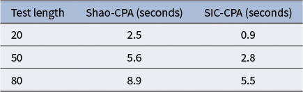
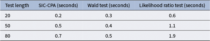
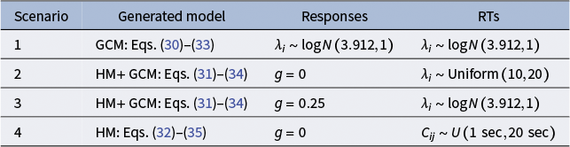


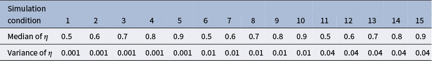


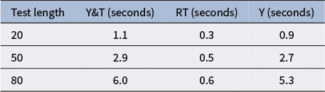


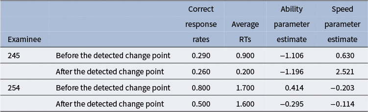


 Open access