


1 Introduction
Item response theory (IRT) is being widely used in the field of psychology, education, and behavioral sciences, for many practical applications, such as data analysis, test equating and linking, developments of standard setting, and computerized adaptive testing (CAT). Numerous IRT models have been developed to take into account various features of item response data (van der Linden & Glas, Reference van der Linden and Glas2010; van der Linden, Reference van der Linden2016). In line with the development and expansion of IRT models, this article addresses two psychometric challenges.
Firstly, most of the IRT models used for test equating, standard setting, and CAT struggle with handling continuous response data. For example, in the age of generative artificial intelligence (AI), measuring skills, such as computer programming, often involves items that are continuously scored (e.g., Gerdes et al., Reference Gerdes, Jeuring and Heeren2010; Maiorana et al., Reference Maiorana, Giordano and Morelli2015; Seo & Cho, Reference Seo and Cho2018). Accurately accrediting test-takers on a reliable and comparable scale requires equating across different test dates, developing a standard setting, or constructing a proficiency scale. In these assessments, item responses can be completion rates, which are the ratio of completed subtasks to the total subtasks, where the number of subtasks often exceeds 10, or even 100. Moreover, continuous response formats, such as slider or visual analog scale (VAS) items, are increasingly used in computer-based assessments (e.g., Attali et al., Reference Attali, Runge, LaFlair, Yancey, Goodwin, Park and von Davier2022; García-Pérez, Reference García-Pérez2024; Gu, Reference Gu2018; Open-Source Psychometrics Project, 2020; Toepoel & Funke, Reference Toepoel and Funke2018; Vall-Llosera et al., Reference Vall-Llosera, Linares-Mustarós, Bikfalvi and Coenders2020). Existing IRT models typically require discretizing continuous responses, leading to a loss of information. Instead, IRT models capable of directly handling continuous responses would provide more appropriate results for test equating and standard setting by preserving the continuous scale of the data.
Secondly, sparse item response data, characterized by a limited number of test-takers for each item or score category, is widely observed in the operational datasets (e.g., Casabianca et al., Reference Casabianca, Donoghue, Shin, Chao and Choi2023; Jones et al., Reference Jones, Smith and Talley2011; Kallinger et al., Reference Kallinger, Scharm, Boecker, Forkmann and Baumeister2019; Mitchell et al., Reference Mitchell, Kallen, Troost, Bragg, Martin-Howard, Moldovan and Carlozzi2023). For example, ordinal response categories (e.g., $x=0, 1, 2, ..., N$
) with few or no observations in certain categories hinder the application of polytomous IRT models, often necessitating post-hoc adjustments, such as collapsing score categories. This can be further exacerbated in the adaptive testing situation, when easy items dominate item banks to ensure test-taker engagement, resulting in sparse data in lower score categories, as most test-takers may get high scores on these items. Furthermore, a balanced incomplete block design (BIBD), which produces a sparse item response matrix, can be preferred to avoid the effect of test fatigue when many items are added to an item bank at once (e.g., Chen et al., Reference Chen, Zheng, Fan and Mo2023). This problem is expected to become more prevalent as item banks can be rapidly expanded through automated item generation (AIG) using large language models (LLMs) (Attali et al., Reference Attali, Runge, LaFlair, Yancey, Goodwin, Park and von Davier2022; Macat International, 2024; Shin et al., Reference Shin, Li, Ryoo and von Davier2024; von Davier et al., Reference von Davier, Runge, Park, Attali, Church, LaFlair, Jiao and Lissitz2024). Additionally, parsimonious IRT models can be beneficial for assessments with underrepresented groups, such as visually impaired students, where only a limited number of students participate in the assessment. In such cases, accurate and stable parameter estimation is threatened, but a parsimonious IRT model can be considered beneficial (Davey & Pitoniak, Reference Davey and Pitoniak2011; O’Neill et al., Reference O’Neill, Gregg and Peabody2020).
$x=0, 1, 2, ..., N$
) with few or no observations in certain categories hinder the application of polytomous IRT models, often necessitating post-hoc adjustments, such as collapsing score categories. This can be further exacerbated in the adaptive testing situation, when easy items dominate item banks to ensure test-taker engagement, resulting in sparse data in lower score categories, as most test-takers may get high scores on these items. Furthermore, a balanced incomplete block design (BIBD), which produces a sparse item response matrix, can be preferred to avoid the effect of test fatigue when many items are added to an item bank at once (e.g., Chen et al., Reference Chen, Zheng, Fan and Mo2023). This problem is expected to become more prevalent as item banks can be rapidly expanded through automated item generation (AIG) using large language models (LLMs) (Attali et al., Reference Attali, Runge, LaFlair, Yancey, Goodwin, Park and von Davier2022; Macat International, 2024; Shin et al., Reference Shin, Li, Ryoo and von Davier2024; von Davier et al., Reference von Davier, Runge, Park, Attali, Church, LaFlair, Jiao and Lissitz2024). Additionally, parsimonious IRT models can be beneficial for assessments with underrepresented groups, such as visually impaired students, where only a limited number of students participate in the assessment. In such cases, accurate and stable parameter estimation is threatened, but a parsimonious IRT model can be considered beneficial (Davey & Pitoniak, Reference Davey and Pitoniak2011; O’Neill et al., Reference O’Neill, Gregg and Peabody2020).
Several IRT models have been proposed to deal with these challenges (see Section 2.3). However, they may not be suitable for operational applications of IRT in practice. Potential issues include assumption misalignment (Noel & Dauvier, Reference Noel and Dauvier2007; Samejima, Reference Samejima1973), infeasible parameter estimation (Müller, Reference Müller1987; Verhelst, Reference Verhelst, Veldkamp and Sluijter2019), and complex model interpretation (Müller, Reference Müller1987; Samejima, Reference Samejima1973). Additionally, some models are based on factor analysis (FA) (Ferrando, Reference Ferrando2001; Mellenbergh, Reference Mellenbergh1994), and others focus on some special types of item responses (Chen et al., Reference Chen, Silva Filho, Prudencio, Diethe and Flach2019; Kloft et al., Reference Kloft, Hartmann, Voss and Heck2023; Molenaar et al., Reference Molenaar, Cúri and Bazán2022; Noel, Reference Noel2014).
As a novel alternative approach, this article aims to propose a continuous-response IRT model: extended two-parameter logistic (E2PL) item response model, which can handle continuous item responses and sparse item responses. The E2PL extends the original two-parameter logistic model (2PL: Birnbaum, Reference Birnbaum, Lord and Novick1968) by incorporating an additional precision parameter that accounts for error, modeled using a beta distribution.
The proposed model offers several advantages. First, by benchmarking the generalized latent variable modeling framework (Skrondal & Rabe-Hesketh, Reference Skrondal and Rabe-Hesketh2004), although it does not strictly belong to the framework as it should be (see Section 3.3), its structure and interpretation are closely aligned with existing models, such as standard IRT and FA. For instance, indices analogous to communality and unique variance in FA can be easily derived, and parameters, such as factor loadings and intercepts, are explicitly specified. Consequently, the item parameters (i.e., item discrimination, difficulty, and precision) are straightforward to interpret. The discrimination and difficulty parameters retain interpretations similar to the 2PL model, while the precision parameter governs the error component. Specifically, the inverse of the precision parameter plays a role analogous to that of the dispersion parameter in the generalized linear model (GLM) framework (Ferrari & Cribari-Neto, Reference Ferrari and Cribari-Neto2004; McCullagh & Nelder, Reference McCullagh and Nelder1989; Skrondal & Rabe-Hesketh, Reference Skrondal and Rabe-Hesketh2004). Second, the error term’s beta distribution, which is the conjugate prior of binomial distribution, enables the model to accommodate a wide range of response distributions, including skewed or zero-one-inflated data. Third, it can effectively handle sparse score categories of polytomous item response data by transforming ordinal responses to a continuous scale (as demonstrated in Section 6). Being parsimonious, the E2PL can yield better model-data fit than conventional polytomous IRT models, especially when items have many score categories and sparse data limits the accuracy of parameter estimation. Lastly, the bell-shaped item information function of the E2PL is a useful feature that is expected to be used in adaptive testing to administer an item that provides maximum information.
The remainder of this article is organized as follows. Section 2 provides an overview of IRT and reviews existing IRT models for continuous responses. Section 3 presents the mathematical formulation of the E2PL with visual illustrations and through a comparison with the 2PL, discusses its differences from Noel & Dauvier (Reference Noel and Dauvier2007)’s model, and explicates its theoretical item response distribution. A simulation study in Section 4 evaluates the stability of the estimation algorithm, parameter recovery, and the computation time of parameter estimation. Sections 5 and 6 illustrate the application of the E2PL to empirical continuous response data and sparse polytomous data, respectively. Lastly, Section 7 discusses the E2PL’s potential and limitations and concludes the article. Detailed parameter estimation procedures are presented in the Appendix.
2 IRT and continuous item responses
2.1 IRT
Unlike classical test theory (CTT), which relies on summed scores, many IRT models use mathematical formulations that allow both item parameters (item characteristics) and ability parameters (test-takers’ latent proficiencies) to be calibrated and interpreted on a common scale. Furthermore, with appropriate scale conversions and test designs, scores from different tests can be adjusted and compared on a common scale, a process known as linking, equating, or vertical scaling, depending on the measurement context (Kolen, Reference Kolen2004). These features make IRT favorable for assessment developers and measurement practitioners in developing, administering, analyzing, and reporting tests. Additionally, assuming the item parameters in the item bank are accurate, IRT provides the foundational framework of adaptive testing, which enables test assembly, test selection, test stopping, and proficiency estimation.
2.1.1 2PL model
As one of the most popular IRT models and for its direct connection to the E2PL, we briefly review the 2PL (Birnbaum, Reference Birnbaum, Lord and Novick1968). Assuming one dichotomous item response $x\in \{0,1\}$
from a single test-taker for brevity, the probability of a correct response (
$x\in \{0,1\}$
from a single test-taker for brevity, the probability of a correct response ( $x=1$
) can be expressed as follows:
$x=1$
) can be expressed as follows:
 $$ \begin{align} P(x=1 | \theta, a, b) = \frac{e^{a(\theta-b)}}{1+e^{a(\theta-b)}}, \end{align} $$
where $\theta $
, a, and b are ability parameter, item discrimination parameter, and item difficulty parameter, respectively. Depending on varying
$\theta $
, a, and b are ability parameter, item discrimination parameter, and item difficulty parameter, respectively. Depending on varying $\theta $
values, the probability of a correct response ranges from 0 to 1, exhibiting an S-shaped curve as in Panel (a) of Figure 1. The item difficulty parameter b determines the inflection point of the symmetric curve at which the probability becomes
$\theta $
values, the probability of a correct response ranges from 0 to 1, exhibiting an S-shaped curve as in Panel (a) of Figure 1. The item difficulty parameter b determines the inflection point of the symmetric curve at which the probability becomes $0.5$
, and the item discrimination parameter a determines the steepness of the curve.
$0.5$
, and the item discrimination parameter a determines the steepness of the curve.
ICFs and item information functions of the 2PL.
Note: For illustrative purposes, values of item parameters are set to $a=1$
and
$a=1$
and $b=0$
for the solid lines and to
$b=0$
for the solid lines and to $a=2$
and
$a=2$
and $b=-2$
for the dotted lines.
$b=-2$
for the dotted lines.

Scale transformation
If a, b, and $\theta $
in Equation (1) are replaced with
$\theta $
in Equation (1) are replaced with $a^{*}=a/\alpha $
,
$a^{*}=a/\alpha $
, $b^{*}=\alpha b +\beta $
, and
$b^{*}=\alpha b +\beta $
, and $\theta ^{*}=\alpha \theta +\beta $
, it is always satisfied that
$\theta ^{*}=\alpha \theta +\beta $
, it is always satisfied that $P(x=1 | \theta , a, b) = P(x=1 | \theta ^{*}, a^{*}, b^{*})$
for arbitrary
$P(x=1 | \theta , a, b) = P(x=1 | \theta ^{*}, a^{*}, b^{*})$
for arbitrary $\alpha $
and
$\alpha $
and $\beta $
. Using this linear transformation, test linking, equating, and vertical scaling can be achieved in a more flexible and interpretable way.
$\beta $
. Using this linear transformation, test linking, equating, and vertical scaling can be achieved in a more flexible and interpretable way.
Information function
Supposing $P(\theta )=P(x=1 | \theta , a, b)$
, the item information function
$P(\theta )=P(x=1 | \theta , a, b)$
, the item information function $I(\theta )$
can be written as follows:
$I(\theta )$
can be written as follows:
 $$ \begin{align} I(\theta)=a^{2}P(\theta)\left(1-P(\theta)\right), \end{align} $$
which is Panel (b) of Figure 1. The item information function has its highest value at $\theta =b$
, and the peak of the function gets higher with a larger a value. The function tapers to 0 as
$\theta =b$
, and the peak of the function gets higher with a larger a value. The function tapers to 0 as $\theta $
diverges to positive or negative infinity. The bell-shape of the function implies that the amount of information is concentrated around
$\theta $
diverges to positive or negative infinity. The bell-shape of the function implies that the amount of information is concentrated around $\theta =b$
. In particular, the item information function provides useful insight about the range of targeted test-takers’ ability levels during the assessment design and CAT.
$\theta =b$
. In particular, the item information function provides useful insight about the range of targeted test-takers’ ability levels during the assessment design and CAT.
Asymptotic standard error
Since the asymptotic standard error of the ability parameter estimate $\hat {\theta }$
is
$\hat {\theta }$
is $[\sum _{i}{I_{i}(\hat {\theta })}]^{-1/2}$
, where i denotes the item, the amount of information directly affects the accuracy of the ability parameter estimate.
$[\sum _{i}{I_{i}(\hat {\theta })}]^{-1/2}$
, where i denotes the item, the amount of information directly affects the accuracy of the ability parameter estimate.
2.2 Modeling continuous item responses
Along with the advancement of IRT to address a variety of measurement challenges, the introduction of diverse item formats and assessment designs has further driven the development of models capable of handling various types of item responses. These include, but are not limited to, dichotomous, polytomous, and continuous responses.
While numerous IRT models have been developed to address dichotomous and polytomous data, relatively few models have been proposed to flexibly accommodate continuous item responses. One reason for this lag is the traditional compartmentalization of latent variable modeling, which generally categorizes IRT as a framework for analyzing discrete observed variables alongside continuous latent variables (Bartholomew et al., Reference Bartholomew, Knott and Moustaki2011). According to this classification, continuous observed variables (i.e., continuous item responses) are typically handled using FA. Although this distinction is not a strict rule (Cai, Reference Cai2012), it is often presented in introductory texts on latent variable modeling for its conceptual simplicity. This convention may have led researchers to either apply FA or discrete-response IRT models to continuous-response data.
Another factor contributing to the slower development of continuous-response IRT models is the historical reliance on paper-based assessments, where items are predominantly scored dichotomously or polytomously. It is only more recently, with advancements in information and computer technologies, that continuous item formats have gained broader use in practice (e.g., Attali et al., Reference Attali, Runge, LaFlair, Yancey, Goodwin, Park and von Davier2022; García-Pérez, Reference García-Pérez2024; Gu, Reference Gu2018; Open-Source Psychometrics Project, 2020; Toepoel & Funke, Reference Toepoel and Funke2018).
2.3 Existing models for continuous item responses
This section reviews existing IRT models for continuous item responses. Each model has its own distinct characteristics and purposes, but they may present limitations for test development, linking, or equating due to their parameterization, underlying assumptions, or structural features. Certain models are only briefly mentioned here, as they are less relevant to the scope of this article: Mellenbergh (Reference Mellenbergh1994) and Ferrando (Reference Ferrando2001) adopted the identity link function in modeling continuous response, a typical choice within the FA framework, Noel (Reference Noel2014) proposed a model for unfolding responses using the Dirichlet distribution, Chen et al. (Reference Chen, Silva Filho, Prudencio, Diethe and Flach2019)’s model assumes a bounded latent space, and Kloft et al. (Reference Kloft, Hartmann, Voss and Heck2023) focused on modeling interval responses on a continuous range using the Dirichlet distribution.
-
• Samejima (Reference Samejima1973)’s model: By taking the number of categories in the graded response model (Samejima, Reference Samejima1969) to infinity, the model postulates an ability parameter and three item parameters: item discrimination, difficulty, and scaling. When a 2PL-type parameterization is applied, the modified difficulty parameter is a combination of the scaling parameter and the original difficulty parameter. The model is based on the normality assumption on the logit-transformed response, and item information is constant across the latent $\theta $
scale.
$\theta $
scale. -
• Müller (Reference Müller1987)’s model: Similar to Samejima (Reference Samejima1973)’s model, the model is an extension of Andrich (Reference Andrich1982)’s rating scale model by taking the number of categories to infinity. The parameters of interest are ability, item difficulty, and item dispersion. As a Rasch-type model, it holds the specific objectivity property, enabling conditional maximum likelihood estimation. However, parameter estimation may not be practically feasible (Verhelst, Reference Verhelst, Veldkamp and Sluijter2019) and the absence of the item discrimination parameter can present limitations in practical applications. In addition, item responses are projected on the latent scale using a uniform distribution.
-
• Noel & Dauvier (Reference Noel and Dauvier2007)’s model: The model utilizes the beta distribution in modeling continuous bounded response, and has ability, item difficulty, and item dispersion parameters. In contrast to the other models that project item responses on the latent space, the model directly handles item responses on their original domain using the beta distribution. The model assumes that the responses are generated from an interpolation mechanism. This model has the most relevant feature to the E2PL, thus, their relationships are discussed in Section 3.4.
-
• Verhelst (Reference Verhelst, Veldkamp and Sluijter2019)’s model: The model is a direct extension of the Rasch model (Rasch, Reference Rasch1960), having only ability parameter and item difficulty parameter. Despite its simplicity, the model postulates neither probabilistic distribution nor an additional parameter to account for the continuity of responses, such as the scaling or dispersion parameter in the other models discussed above. Furthermore, parameter estimation may not be practically feasible (Verhelst, Reference Verhelst, Veldkamp and Sluijter2019), and the effectiveness of the practical application has not been examined.
-
• Molenaar et al. (Reference Molenaar, Cúri and Bazán2022)’s model: Under the assumption that 0s and 1s are inflated, 0s and 1s are separated from the other responses through mixture modeling. Then, responses between 0 and 1 (
$0<x<1$
) can be modeled with any type of model listed above. However, considering that seemingly zero-one-inflated data can be properly modeled by a beta distribution, it is challenging to tell whether 0s and 1s are truly inflated.


Building on the review of existing methods, the practical need for a new model can be formally motivated as follows. Suppose we are designing an assessment that includes both dichotomous and continuous items, using the 2PL model for dichotomous items to capture item discrimination and difficulty. This structure can be observed in practice, for instance, in programming assessments that combine multiple-choice questions (scored dichotomously) with coding tasks evaluated as percentage-correct (continuous). In this context, the zero-one inflated model by Molenaar et al. (Reference Molenaar, Cúri and Bazán2022) is not suitable for general measurement purposes. Additionally, the models proposed by Müller (Reference Müller1987), Verhelst (Reference Verhelst, Veldkamp and Sluijter2019), and Noel & Dauvier (Reference Noel and Dauvier2007) do not incorporate item discrimination parameters, making them incompatible with the 2PL framework. The interpolation mechanism assumed in Noel & Dauvier (Reference Noel and Dauvier2007) is also unlikely to be appropriate for item responses such as percentage-correct scores. Finally, while Samejima (Reference Samejima1973)’s model includes discrimination and difficulty parameters, they are not aligned with those of the 2PL model. In particular, its expected value is given by $\sigma (\nu (\theta - b))$
(Wang & Zeng, Reference Wang and Zeng1998), where
$\sigma (\nu (\theta - b))$
(Wang & Zeng, Reference Wang and Zeng1998), where $\nu $
is a scaling parameter and
$\nu $
is a scaling parameter and $\sigma (\cdot )$
denotes the sigmoid function, whereas the 2PL uses
$\sigma (\cdot )$
denotes the sigmoid function, whereas the 2PL uses $\sigma (a(\theta - b))$
as in Equation (1), with a representing item discrimination. Therefore, a new model that is compatible with the 2PL, as well as capable of handling continuous item responses, is required.
$\sigma (a(\theta - b))$
as in Equation (1), with a representing item discrimination. Therefore, a new model that is compatible with the 2PL, as well as capable of handling continuous item responses, is required.
3 E2PL model
3.1 Formulation of the E2PL
3.1.1 Model equations
Moving from the 2PL (see Equation (1)) to the E2PL, we make a transition from binary to continuous response. Below, the response x takes a real number ( $0<x<1$
), thus, the modeled value is no longer a probability for the Bernoulli distribution but an observable quantity. The model equations can be written as follows:
$0<x<1$
), thus, the modeled value is no longer a probability for the Bernoulli distribution but an observable quantity. The model equations can be written as follows:
 $$ \begin{align} \begin{aligned} x &= \frac{e^{a(\theta-b)}}{1+e^{a(\theta-b)}} + \varepsilon \\ &= \mu + \varepsilon, \end{aligned} \end{align} $$
 $$ \begin{align} \mu = E\left[x | \theta, a, b, \nu \right] = \frac{\exp{(a(\theta-b))}}{1+\exp{(a(\theta-b))}}, \end{align} $$
 $$ \begin{align} Var\left[x | \theta, a, b, \nu\right] = Var\left[\varepsilon | \theta, a, b, \nu\right] = \frac{\mu(1-\mu)}{\nu+1}, \end{align} $$
and
 $$ \begin{align} \begin{aligned} f(\varepsilon \mid \mu, \nu) = \frac{\Gamma(\nu)}{\Gamma(\nu\mu)\Gamma(\nu(1-\mu))}{(\varepsilon + \mu)}^{\nu\mu-1}(1- \varepsilon - \mu)^{\nu(1-\mu)-1} \\ (\varepsilon + \mu) \sim Beta(\nu\mu, \nu(1-\mu)). \end{aligned} \end{align} $$
The expected response $\mu $
is equal to the model equation of the 2PL (Equation (1)). Particularly, the error term
$\mu $
is equal to the model equation of the 2PL (Equation (1)). Particularly, the error term $\varepsilon $
is introduced to account for the continuous nature of the response using a beta distribution. Through a comparison with the 2PL, Section 3.2.1 illustrates how this error term reflects the continuity. The error term follows a shifted beta distribution where the amount of the shift is
$\varepsilon $
is introduced to account for the continuous nature of the response using a beta distribution. Through a comparison with the 2PL, Section 3.2.1 illustrates how this error term reflects the continuity. The error term follows a shifted beta distribution where the amount of the shift is $-\mu $
(
$-\mu $
( $-\mu < \varepsilon < 1-\mu $
). The precision parameter
$-\mu < \varepsilon < 1-\mu $
). The precision parameter $\nu $
can represent the degree to which the density is concentrated around
$\nu $
can represent the degree to which the density is concentrated around $\mu $
. Using Equations (3) and (6), the model can be rewritten in a probabilistic form:
$\mu $
. Using Equations (3) and (6), the model can be rewritten in a probabilistic form:
 $$ \begin{align} P(x | \theta, a, b, \nu) &= \frac{\Gamma(\nu)}{\Gamma(\nu\mu)\Gamma(\nu(1-\mu))}x^{\nu\mu-1}(1-x)^{\nu(1-\mu)-1}.\end{align} $$
3.1.2 Information function
The item information function of the E2PL can be expressed using trigamma function $\psi _{1}(\cdot )$
:
$\psi _{1}(\cdot )$
:
 $$ \begin{align} \begin{aligned} I(\theta) &= \left(a\nu\mu(1-\mu)\right)^{2}\left[\psi_{1}(\nu\mu)+\psi_{1}(\nu(1-\mu))\right]. \end{aligned} \end{align} $$
In general, the item information function resembles a bell-shaped curve, peaking at $\theta =b$
. However, its shape can vary depending on the precision parameter
$\theta =b$
. However, its shape can vary depending on the precision parameter $\nu $
. When
$\nu $
. When $\nu $
is close to 3, the function can take a W-shaped form, whereas for values of
$\nu $
is close to 3, the function can take a W-shaped form, whereas for values of $\nu $
less than 2, it tends to look like a bell-shaped curve flipped upside down. Notably, even with small values of
$\nu $
less than 2, it tends to look like a bell-shaped curve flipped upside down. Notably, even with small values of $\nu $
, the item information in the E2PL model is greater than that of the 2PL model, assuming the same a and b parameters are used for both. The greater information of the E2PL can be attributed to its more refined response structure compared with binary responses. Unlike many other dichotomous or polytomous models, the information function in the E2PL does not approach zero as
$\nu $
, the item information in the E2PL model is greater than that of the 2PL model, assuming the same a and b parameters are used for both. The greater information of the E2PL can be attributed to its more refined response structure compared with binary responses. Unlike many other dichotomous or polytomous models, the information function in the E2PL does not approach zero as $\theta $
approaches
$\theta $
approaches $\pm \infty $
, instead asymptotically approaching
$\pm \infty $
, instead asymptotically approaching $a^2$
from below.
$a^2$
from below.
3.1.3 Likelihood
We can add subscripts to the equations to express a likelihood function of data. Letting $j = 1, 2, ..., N$
denote test takers and
$j = 1, 2, ..., N$
denote test takers and $i_{j} \in I_{j}$
be an ith item among
$i_{j} \in I_{j}$
be an ith item among $I_{j}$
items that the jth test taker responded to, the likelihood can be expressed as follows:
$I_{j}$
items that the jth test taker responded to, the likelihood can be expressed as follows:
 $$ \begin{align} \mathcal{L} = \prod_{j=1}^{N}\prod_{i_{j}\in I_{j}} P\left(x_{ji_{j}} | \theta_{j}, a_{i_{j}}, b_{i_{j}}, \nu_{i_{j}}\right). \end{align} $$
The individual item response probabilities (Equation (7)) are multiplied under the assumptions that responses within individuals are independent conditional on the latent trait level $\theta _j$
(i.e., the local independence assumption) and that responses are statistically independent across individuals.
$\theta _j$
(i.e., the local independence assumption) and that responses are statistically independent across individuals.
3.1.4 Model-data fit and standardized residuals
Following the approach proposed by Ferrari & Cribari-Neto (Reference Ferrari and Cribari-Neto2004) in the context of beta regression, the standardized residual for test taker j and item i can be computed as:
 $$ \begin{align} r_{ji}=\frac{x_{ji} - \hat{\mu}_{ji}} {\sqrt{Var\left(x_{ji} \right)}}, \end{align} $$
where $\hat {\mu }_{ji}=\left (1+\exp \left (-\hat {a}_{i}(\hat {\theta }_j-\hat {b}_{i})\right )\right )^{-1}$
and
$\hat {\mu }_{ji}=\left (1+\exp \left (-\hat {a}_{i}(\hat {\theta }_j-\hat {b}_{i})\right )\right )^{-1}$
and $Var\left (x_{ji} \right )=\frac {\hat {\mu }_{ji}(1-\hat {\mu }_{ji})}{\hat {\nu }_{i}+1}$
are from Equations (4) and (5). Residual analysis based on this formulation can provide evidence of model misspecification.
$Var\left (x_{ji} \right )=\frac {\hat {\mu }_{ji}(1-\hat {\mu }_{ji})}{\hat {\nu }_{i}+1}$
are from Equations (4) and (5). Residual analysis based on this formulation can provide evidence of model misspecification.
The overall model-data fit can be assessed using a pseudo $R^2$
, defined as the squared correlation between the log-odds of
$R^2$
, defined as the squared correlation between the log-odds of $\hat {\mu }_{ji}$
and the log-odds of
$\hat {\mu }_{ji}$
and the log-odds of $x_{ji}$
(Ferrari & Cribari-Neto, Reference Ferrari and Cribari-Neto2004). Additionally, K-fold cross-validation provides a more robust estimate of predictive performance. In this case, the log-likelihood under the beta distribution or the root mean squared error (RMSE) of the standardized residuals (i.e.,
$x_{ji}$
(Ferrari & Cribari-Neto, Reference Ferrari and Cribari-Neto2004). Additionally, K-fold cross-validation provides a more robust estimate of predictive performance. In this case, the log-likelihood under the beta distribution or the root mean squared error (RMSE) of the standardized residuals (i.e., $\sqrt {\frac {1}{T}\sum _{j}\sum _{i}r^{2}_{ji}}$
) can serve as a loss function, where T is the total number of item responses evaluated.
$\sqrt {\frac {1}{T}\sum _{j}\sum _{i}r^{2}_{ji}}$
) can serve as a loss function, where T is the total number of item responses evaluated.
Accordingly, for the current version of the E2PL, we advocate the use of standardized residuals, pseudo $R^2$
, and K-fold cross-validation for evaluating model fit, due to their interpretability. More advanced diagnostic and fit assessment methods (e.g., Espinheira et al., Reference Espinheira, da Silva, Silva, de Oliveira Silva and Ospina2019; Espinheira et al., Reference Espinheira, Ferrari and Cribari-Neto2008; Smithson & Verkuilen, Reference Smithson and Verkuilen2006) may be appropriate for future extensions of E2PL.
$R^2$
, and K-fold cross-validation for evaluating model fit, due to their interpretability. More advanced diagnostic and fit assessment methods (e.g., Espinheira et al., Reference Espinheira, da Silva, Silva, de Oliveira Silva and Ospina2019; Espinheira et al., Reference Espinheira, Ferrari and Cribari-Neto2008; Smithson & Verkuilen, Reference Smithson and Verkuilen2006) may be appropriate for future extensions of E2PL.
3.1.5 Parameter estimation
Item parameters can be estimated through marginal maximum likelihood using the expectation–maximization algorithm (MML-EM: Bock & Aitkin, Reference Bock and Aitkin1981), where the marginal likelihood is obtained by integrating the likelihood $\mathcal {L}$
with respect to
$\mathcal {L}$
with respect to $\theta $
. Conventionally, the
$\theta $
. Conventionally, the $\theta $
distribution is assumed to follow the standard normal distribution. Several types of scores can be used as ability parameter estimates, such as expected a posteriori (EAP), maximum likelihood estimate (MLE), or weighted likelihood estimate (WLE). Details of the parameter estimation are provided in the Appendix.
$\theta $
distribution is assumed to follow the standard normal distribution. Several types of scores can be used as ability parameter estimates, such as expected a posteriori (EAP), maximum likelihood estimate (MLE), or weighted likelihood estimate (WLE). Details of the parameter estimation are provided in the Appendix.
3.2 Item characteristic function (ICF)
3.2.1 Comparison with the 2PL
Within the generalized latent variable modeling framework (Skrondal & Rabe-Hesketh, Reference Skrondal and Rabe-Hesketh2004), both FA and IRT models can be expressed in the form $\lambda (\mu ) = a\theta + c$
, where
$\lambda (\mu ) = a\theta + c$
, where $\lambda (\cdot )$
denotes the link function, typically the identity link for FA and the logit link for IRT. In this formulation, the slope parameter a corresponds to the factor loading, and c represents the intercept. Specifically, in the 2PL model, a is interpreted as item discrimination, while item difficulty is given by
$\lambda (\cdot )$
denotes the link function, typically the identity link for FA and the logit link for IRT. In this formulation, the slope parameter a corresponds to the factor loading, and c represents the intercept. Specifically, in the 2PL model, a is interpreted as item discrimination, while item difficulty is given by $b = -\frac {c}{a}$
. The E2PL model adopts this same structural formulation, allowing for analogous interpretations of the a and b parameters. However, the key distinction lies in the modeling of the dispersion structure: the 2PL model assumes a Bernoulli distribution for the observed responses, whereas the E2PL employs a beta distribution. This difference in distributional assumption differentiates the two models.
$b = -\frac {c}{a}$
. The E2PL model adopts this same structural formulation, allowing for analogous interpretations of the a and b parameters. However, the key distinction lies in the modeling of the dispersion structure: the 2PL model assumes a Bernoulli distribution for the observed responses, whereas the E2PL employs a beta distribution. This difference in distributional assumption differentiates the two models.
Figure 2 visually illustrates similarities and differences between the 2PL and the E2PL. Due to their common item discrimination and difficulty parameters, the ICF of the 2PL in Panel (a) and the $\mu $
curve of the E2PL in Panel (b) are identical. Thus, item interpretations of the two models would be similar or, for convenience, interchangeable. In addition, an identical linear transformation can be carried out for the two models for test linking or equating. Therefore, for mixed-format data of dichotomous and continuous item responses, adopting the pair of the 2PL and the E2PL simplifies the model interpretation and the scale transformation.
$\mu $
curve of the E2PL in Panel (b) are identical. Thus, item interpretations of the two models would be similar or, for convenience, interchangeable. In addition, an identical linear transformation can be carried out for the two models for test linking or equating. Therefore, for mixed-format data of dichotomous and continuous item responses, adopting the pair of the 2PL and the E2PL simplifies the model interpretation and the scale transformation.
ICFs of the 2PL and the E2PL.
Note: For the illustration, values of item parameters are set to $a=1$
and
$a=1$
and $b=0$
for both functions and
$b=0$
for both functions and $\nu =10$
for the E2PL. The y-axis is probability in Panel (a) and response in Panel (b). In Panel (b), the
$\nu =10$
for the E2PL. The y-axis is probability in Panel (a) and response in Panel (b). In Panel (b), the ![]() indicate 95% interval conditional on
indicate 95% interval conditional on $\theta $
. The
$\theta $
. The ![]() are probability densities of continuous item responses for the selected
are probability densities of continuous item responses for the selected $\theta $
values of -2, -1, 0, 1, and 2. The
$\theta $
values of -2, -1, 0, 1, and 2. The ![]() on the
on the $\mu $
-curve indicate the means of the densities.
$\mu $
-curve indicate the means of the densities.

Compared with the 2PL’s ICF, the ICF of the E2PL in Panel (b) of Figure 2 includes the blue and gray curves to display the beta distribution, the error component of the E2PL. In line with the change of the y-axis from $probability$
to
$probability$
to $response$
, the error term of the E2PL accounts for the continuous scale of the response. The distribution (
$response$
, the error term of the E2PL accounts for the continuous scale of the response. The distribution (![]() ) and the 95% interval (
) and the 95% interval (![]() ) illustrate how the error distribution changes according to
) illustrate how the error distribution changes according to $\theta $
.
$\theta $
.
3.2.2 Role of the item parameters
Figure 3 visually illustrates how item parameters influence ICFs in the E2PL. The upper left and right panels show that the effects of the a and b parameters on ICFs are structurally identical to those in the 2PL model: the a parameter alters the steepness of ICFs and the b parameter shifts ICFs along the $\theta $
-axis. However, unlike the 2PL, where the Y-axis represents probability, the E2PL models the response directly on a continuous scale. Accordingly, the a parameter determines the slope of the expected response (i.e., the
$\theta $
-axis. However, unlike the 2PL, where the Y-axis represents probability, the E2PL models the response directly on a continuous scale. Accordingly, the a parameter determines the slope of the expected response (i.e., the $\mu $
curve), and the expected response reaches 0.5 when
$\mu $
curve), and the expected response reaches 0.5 when $\theta = b$
.
$\theta = b$
.
ICFs of the E2PL with varying parameter values.
Note: The ![]() indicate 95% interval conditional on
indicate 95% interval conditional on $\theta $
. The
$\theta $
. The ![]() are probability densities of continuous item responses for selected
are probability densities of continuous item responses for selected $\theta $
values of -2, -1, 0, 1, and 2. The
$\theta $
values of -2, -1, 0, 1, and 2. The ![]() on the
on the $\mu $
-curve indicate the means of the densities.
$\mu $
-curve indicate the means of the densities.

Focusing now on the role of the precision parameter $\nu $
, when the expected response curves (solid black lines) are held constant, the error distributions (
$\nu $
, when the expected response curves (solid black lines) are held constant, the error distributions (![]() ) are also identical across panels with the same
) are also identical across panels with the same $\nu $
. For example, in the upper-left panel at
$\nu $
. For example, in the upper-left panel at $\theta = 0$
and the upper-right panel at
$\theta = 0$
and the upper-right panel at $\theta = 1$
, the distributions are identical because both yield an expected response of
$\theta = 1$
, the distributions are identical because both yield an expected response of $\mu = 0.5$
under the same precision level
$\mu = 0.5$
under the same precision level $\nu = 10$
.
$\nu = 10$
.
To illustrate the effect of the precision parameter, the precision parameter $\nu $
is varied between the lower left and right panels. It can be seen that the precision parameter modified only the error variances (
$\nu $
is varied between the lower left and right panels. It can be seen that the precision parameter modified only the error variances (![]() ) and the width of the interval (
) and the width of the interval (![]() ). In brief, after the mean curve (solid black curves) is determined by the a and b parameters, the precision parameter
). In brief, after the mean curve (solid black curves) is determined by the a and b parameters, the precision parameter $\nu $
determines the dispersion, or concentration, of ICFs.
$\nu $
determines the dispersion, or concentration, of ICFs.
3.3 Communality and unique dispersion
The formulation of the E2PL is well-aligned with the generalized latent variable modeling framework (Skrondal & Rabe-Hesketh, Reference Skrondal and Rabe-Hesketh2004), as it models the mean structure $\mu $
using the logit link function and introduces the precision parameter
$\mu $
using the logit link function and introduces the precision parameter $\nu $
to handle the dispersion of data. Here, we use the term dispersion instead of variance to indicate the role of
$\nu $
to handle the dispersion of data. Here, we use the term dispersion instead of variance to indicate the role of $\nu $
, since statistical variance of the beta distribution depends on
$\nu $
, since statistical variance of the beta distribution depends on $\mu $
as in Equation (5). Meanwhile, the beta distribution does not provide a statistically independent structure between
$\mu $
as in Equation (5). Meanwhile, the beta distribution does not provide a statistically independent structure between $\mu $
and
$\mu $
and $\nu $
(Ferrari & Cribari-Neto, Reference Ferrari and Cribari-Neto2004), which differentiates the E2PL from the generalized latent variable modeling framework (McCullagh & Nelder, Reference McCullagh and Nelder1989; Skrondal & Rabe-Hesketh, Reference Skrondal and Rabe-Hesketh2004). However, this is a desirable property that allows the model to account for the effects of the item parameters during the calculation of the residual dispersion represented by
$\nu $
(Ferrari & Cribari-Neto, Reference Ferrari and Cribari-Neto2004), which differentiates the E2PL from the generalized latent variable modeling framework (McCullagh & Nelder, Reference McCullagh and Nelder1989; Skrondal & Rabe-Hesketh, Reference Skrondal and Rabe-Hesketh2004). However, this is a desirable property that allows the model to account for the effects of the item parameters during the calculation of the residual dispersion represented by $\nu $
.
$\nu $
.
To mathematically illustrate the aforementioned points, let $\nu _{\text {pre}}=(\frac {\bar {X}(1-\bar {X})}{s^2}-1)$
be the degree of precision for an item before fitting the E2PL with sample mean
$\nu _{\text {pre}}=(\frac {\bar {X}(1-\bar {X})}{s^2}-1)$
be the degree of precision for an item before fitting the E2PL with sample mean $\bar {X}$
and sample variance
$\bar {X}$
and sample variance $s^2$
, and
$s^2$
, and $\nu _{\text {post}}=\hat {\nu }$
be the estimate of the precision parameter of the item in Equations (3)–(7). The subscripts for the items are omitted for notational brevity. Then, using the FA notation from MacCallum (Reference MacCallum, Millsap and Maydeu-Olivares2009),
$\nu _{\text {post}}=\hat {\nu }$
be the estimate of the precision parameter of the item in Equations (3)–(7). The subscripts for the items are omitted for notational brevity. Then, using the FA notation from MacCallum (Reference MacCallum, Millsap and Maydeu-Olivares2009), $1/\nu _{\text {pre}}$
and
$1/\nu _{\text {pre}}$
and $1/\nu _{\text {post}}$
are analogous to the sample variance
$1/\nu _{\text {post}}$
are analogous to the sample variance $s^2$
and the estimate of the unique variance
$s^2$
and the estimate of the unique variance $\hat {\psi }$
in FA, respectively. As a result, the proportion of the unique dispersion of this item becomes
$\hat {\psi }$
in FA, respectively. As a result, the proportion of the unique dispersion of this item becomes $\frac {1/\nu _{\text {post}}}{1/\nu _{\text {pre}}}=\frac {\nu _{\text {pre}}}{\nu _{\text {post}}}$
, and the communality
$\frac {1/\nu _{\text {post}}}{1/\nu _{\text {pre}}}=\frac {\nu _{\text {pre}}}{\nu _{\text {post}}}$
, and the communality $(1-\frac {\nu _{\text {pre}}}{\nu _{\text {post}}})$
indicates the proportion of the uncertainty explained by the latent variable. The relationships above are also applicable to multidimensional
$(1-\frac {\nu _{\text {pre}}}{\nu _{\text {post}}})$
indicates the proportion of the uncertainty explained by the latent variable. The relationships above are also applicable to multidimensional $\theta $
.
$\theta $
.
Figure 4 shows an almost linear relationship between the explained dispersion and the expected item information in log scale. This trend well reflects the conventional practice in IRT to take item parameters into account, rather than excluding them when explaining the uncertainty of the data. Notably, the formulation of the communality and unique dispersion, as well as their relationships to the item information, are not subject to the scale transformation in Section 2.1.1, as the transformation does not affect $\mu $
.
$\mu $
.
The relationships between the proportion of explained uncertainty $(1-\frac {\nu _{\text {pre}}}{\nu _{\text {post}}})$
and expected item information
$(1-\frac {\nu _{\text {pre}}}{\nu _{\text {post}}})$
and expected item information $E[I(\theta )]$
.
$E[I(\theta )]$
.
Note: The expected item information values are calculated as $E[I(\theta )]=\int {I(\theta )}\phi (\theta )\, d\theta $
, where
$E[I(\theta )]=\int {I(\theta )}\phi (\theta )\, d\theta $
, where $I(\theta )$
is the item information function in Equation (8) and the standard normal distribution
$I(\theta )$
is the item information function in Equation (8) and the standard normal distribution $\phi (\theta )$
is used as the latent distribution. The figure is obtained from a randomly generated data for 100,000 test takers and 50 items, where
$\phi (\theta )$
is used as the latent distribution. The figure is obtained from a randomly generated data for 100,000 test takers and 50 items, where $\theta \sim N(0,1)$
,
$\theta \sim N(0,1)$
, $a\sim Unif(0.5, 1.5)$
,
$a\sim Unif(0.5, 1.5)$
, $b\sim N(0,0.5)$
, and
$b\sim N(0,0.5)$
, and $\nu \sim Gamma(10,1)$
.
$\nu \sim Gamma(10,1)$
.

3.4 Differences between the E2PL and Noel and Dauvier’s model
It would be worthwhile to clarify the differences between the E2PL and Noel & Dauvier (Reference Noel and Dauvier2007)’s model as they are closely related to one another. Although they introduced a Rasch-type model without item discrimination parameter, it can be easily added to the model. The following discussion assumes Noel and Dauvier’s model with the inclusion of the item discrimination parameter to make a fair comparison.
Item responses of Noel and Dauvier’s model are assumed to be a manifestation of the interpolation mechanism; an interpolation of one weight ( $\alpha $
) pulling a response toward 0 and another weight (
$\alpha $
) pulling a response toward 0 and another weight ( $\beta $
) pulling it toward 1 (i.e.,
$\beta $
) pulling it toward 1 (i.e., $x=\frac {\alpha }{\alpha + \beta }$
), thereby adopting the shape–shape parameterization of the beta distribution. In other words, they modeled the response using
$x=\frac {\alpha }{\alpha + \beta }$
), thereby adopting the shape–shape parameterization of the beta distribution. In other words, they modeled the response using $Beta(\alpha , \beta )$
, where the expected value of the response x is the interpolation of the two parameters (i.e.,
$Beta(\alpha , \beta )$
, where the expected value of the response x is the interpolation of the two parameters (i.e., $E(x)=\frac {\alpha }{\alpha + \beta }$
). In comparison, without assuming a particular mechanism on item responses, the E2PL adopts the mean–precision parameterization, which is a widely used practice in beta regression (Ferrari & Cribari-Neto, Reference Ferrari and Cribari-Neto2004).
$E(x)=\frac {\alpha }{\alpha + \beta }$
). In comparison, without assuming a particular mechanism on item responses, the E2PL adopts the mean–precision parameterization, which is a widely used practice in beta regression (Ferrari & Cribari-Neto, Reference Ferrari and Cribari-Neto2004).
While the conditional means of the two models (i.e., the $\mu $
terms) can be identically expressed using the a and b parameters, the two models differ in their treatment of precision. In the E2PL model, the conditional variance—after accounting for
$\mu $
terms) can be identically expressed using the a and b parameters, the two models differ in their treatment of precision. In the E2PL model, the conditional variance—after accounting for $\mu $
—is solely governed by the precision parameter
$\mu $
—is solely governed by the precision parameter $\nu $
, enabling a clear separation of the error component as shown in Equation (3). In contrast, the conditional variance in Noel and Dauvier’s model remains a function of all item parameters even after conditioning on
$\nu $
, enabling a clear separation of the error component as shown in Equation (3). In contrast, the conditional variance in Noel and Dauvier’s model remains a function of all item parameters even after conditioning on $\mu $
. Following the parameterization of Ferrari & Cribari-Neto (Reference Ferrari and Cribari-Neto2004), the precision parameter in Noel’s model is given by
$\mu $
. Following the parameterization of Ferrari & Cribari-Neto (Reference Ferrari and Cribari-Neto2004), the precision parameter in Noel’s model is given by $2\exp \left (\frac {\tau }{2}\right )\cosh \left (\frac {a(\theta - b)}{2}\right )$
, where
$2\exp \left (\frac {\tau }{2}\right )\cosh \left (\frac {a(\theta - b)}{2}\right )$
, where $\tau $
is an additional parameter to account for dispersion. In the E2PL model, by contrast, the precision is directly represented by
$\tau $
is an additional parameter to account for dispersion. In the E2PL model, by contrast, the precision is directly represented by $\nu $
. Because the precision term in Noel and Dauvier’s model depends on the latent scale, scale transformations and the derivation of quantities, such as communality and unique dispersion, require additional consideration.
$\nu $
. Because the precision term in Noel and Dauvier’s model depends on the latent scale, scale transformations and the derivation of quantities, such as communality and unique dispersion, require additional consideration.
3.5 Distribution of item responses
Each IRT model assumes a particular distribution for item responses. For instance, when the 2PL’s item parameters are $a=1$
and
$a=1$
and $b=0$
and
$b=0$
and $\theta \sim N(0, 1)$
, the expected probability of observing an item response of
$\theta \sim N(0, 1)$
, the expected probability of observing an item response of $x=1$
is 0.5.
$x=1$
is 0.5.
Similarly, the item response distributions of the E2PL can be derived when the latent distribution is specified. Assuming the standard normal distribution on the latent variable, the response distributions can be mathematically expressed as follows:
 $$ \begin{align} \begin{aligned} f(x |a, b, \nu) &= \int_{-\infty}^{\infty}f(x |\theta, a, b, \nu) \phi(\theta) \, d\theta\\ &=\int_{-\infty}^{\infty}{\frac{\Gamma(\nu)}{\Gamma(\nu\mu)\Gamma(\nu(1-\mu))}x^{\nu\mu-1}(1-x)^{\nu(1-\mu)-1}} \phi(\theta) \, d\theta, \end{aligned} \end{align} $$
where the $\mu $
is defined in Equation (4) and
$\mu $
is defined in Equation (4) and $\phi (\theta )$
denotes the standard normal latent distribution. The distribution depends only on item parameters after integrating out the latent variable
$\phi (\theta )$
denotes the standard normal latent distribution. The distribution depends only on item parameters after integrating out the latent variable $\theta $
.
$\theta $
.
Figure 5 shows that skewed or zero-one-inflated response distributions can be generated by the model, as well as bell-shaped distributions. Firstly, when the difficulty parameter b is different from the mean of the latent distribution, a skewed distribution can be formulated. For instance, the mass of the solid line’s density ( $a=1$
,
$a=1$
, $b=-1$
,
$b=-1$
, $\nu =10$
) is more concentrated near 1 than 0, as the item is relatively easy for the population:
$\nu =10$
) is more concentrated near 1 than 0, as the item is relatively easy for the population: $b<E(\theta )=0$
. In comparison, the densities of the dotted and dashed lines (
$b<E(\theta )=0$
. In comparison, the densities of the dotted and dashed lines ( $a=1$
,
$a=1$
, $b=0$
,
$b=0$
, $\nu =10$
;
$\nu =10$
; $a=1$
,
$a=1$
, $b=0$
,
$b=0$
, $\nu =1$
) are both symmetric as their difficulty parameters are equal to the population mean.
$\nu =1$
) are both symmetric as their difficulty parameters are equal to the population mean.
Response distributions of the E2PL.
Note: The distributions are derived from the standard normal latent distribution. The distributions are numerically approximated.

Secondly, zero-one-inflated response distributions can be formulated with a small value of $\nu $
. For example, the dashed line (
$\nu $
. For example, the dashed line ( $a=1$
,
$a=1$
, $b=0$
,
$b=0$
, $\nu =1$
) shows that both 0 and 1 are inflated even when the difficulty parameter b is equal to the population mean. In a strict sense, it may not be an actual zero-one-inflated distribution as the domain of the beta distribution does not contain 0 and 1. However, in practice, responses are almost always rounded to a certain point (e.g., to the nearest hundredth), producing 0s and 1s. Additionally, skewed zero-one-inflated response distributions can be formulated when the precision parameter is small and
$\nu =1$
) shows that both 0 and 1 are inflated even when the difficulty parameter b is equal to the population mean. In a strict sense, it may not be an actual zero-one-inflated distribution as the domain of the beta distribution does not contain 0 and 1. However, in practice, responses are almost always rounded to a certain point (e.g., to the nearest hundredth), producing 0s and 1s. Additionally, skewed zero-one-inflated response distributions can be formulated when the precision parameter is small and $b\ne E(\theta )$
.
$b\ne E(\theta )$
.
3.6 Preprocessing item responses
To apply the E2PL, a simple transformation of item responses is often necessary, when raw data include minimum and maximum values (e.g., 0% and 100%) that fall outside of the domain of the beta distribution, which excludes 0 and 1. For example, item responses collected as percentages typically include these values as minimum and maximum scores.
To adjust raw responses to fit within the beta distribution while preserving their key characteristics, we recommend the preprocessing scheme shown in Figure 6. This approach divides the open interval (0, 1) into equally spaced grids based on the smallest unit of observation in the raw data and maps the raw responses to the midpoints of these grids. For instance, if percentage responses are measured in 1% increments, the raw scores from 0% to 100% are mapped to the midpoints of 101 equally spaced grids: $\{0\%, 1\%, ..., 100\%\} \mapsto \{\frac {0.5}{101}, \frac {1.5}{101}, ..., \frac {100.5}{101}\}$
. Figure 6 visually illustrates this method.
$\{0\%, 1\%, ..., 100\%\} \mapsto \{\frac {0.5}{101}, \frac {1.5}{101}, ..., \frac {100.5}{101}\}$
. Figure 6 visually illustrates this method.
Mapping raw scores on a unit interval.

This transformation is useful in cases where values approach the absolute maximum or minimum, allowing for meaningful representation of such scores. In practical contexts, discrepancies often exist between mathematical maximums, defined as the highest possible score, and practical maximums, which may exhibit slight variations even at the upper boundary. For instance, some maximum scores represent model solutions that are qualitatively distinct from those that merely achieve the highest possible score. A similar rationale applies to minimum scores, such as the differences between zero scores due to blank responses and other minimum scores. This approach supports using the open interval of the beta distribution, rather than the closed interval, to better reflect the nuanced characteristics of item responses near the extremes. Additionally, other transformations, such as slightly adjusting the minimum and maximum values (Noel & Dauvier, Reference Noel and Dauvier2007), could also be applied when they more accurately capture the characteristics of item responses.
Furthermore, this transformation is justifiable when each item comprises multiple subtasks (see Sections 5 and 6). In such cases, a more sophisticated modeling approach, such as the testlet response model (Bradlow et al., Reference Bradlow, Wainer and Wang1999; Wainer et al., Reference Wainer, Bradlow and Wang2007), is often appropriate for accounting for local item dependencies. However, testlet models can be sensitive to sample size constraints, potentially increasing estimation error due to the bias–variance trade-off and threatening the validity of inferences. While more parsimonious models may be preferable under limited sample conditions, standard polytomous IRT models are often not suitable alternatives, as their response categories typically do not align directly with individual subtasks. Thus, the proposed transformation provides a practical alternative to testlet modeling by enabling the use of the E2PL that maintains fidelity to the item structure while avoiding issues associated with small samples.
4 Simulation study
A simulation study is conducted to assess the recovery of item parameters and the stability of the parameter estimates of the E2PL. Data were generated and the model was fitted using the IRTest package in R (Li, Reference Li2025), with evaluation metrics computed using built-in R functions (R Core Team, 2024). The simulation code is publicly available at https://github.com/SeewooLi/E2PL_simulation_study.
4.1 Data generation and model-fitting
The simulation study utilizes a set of 12 items, designed as the factorial combination of the following item parameters: discrimination ( $a \in \{0.5, 1\}$
), difficulty (
$a \in \{0.5, 1\}$
), difficulty ( $b \in \{-1, 0, 1\}$
), and precision (
$b \in \{-1, 0, 1\}$
), and precision ( $\nu \in \{5, 10\}$
). Sample sizes of 250, 500, and 1000 are used, and for each sample size, 200 sets of item response data are generated based on the specified item parameters.
$\nu \in \{5, 10\}$
). Sample sizes of 250, 500, and 1000 are used, and for each sample size, 200 sets of item response data are generated based on the specified item parameters.
Biases and RMSEs in parameter recovery

Model fitting is conducted using the IRTest package (Li, Reference Li2025). A custom function IRTest_ Cont, which is developed for this study, implements the MML-EM procedure (Bock & Aitkin, Reference Bock and Aitkin1981). Convergence of the MML-EM procedure is defined as the point at which the maximum change in parameter estimates falls below 0.0001 within a maximum of 200 EM iterations, ensuring robust model fitting in this simulation. To address the challenge of directly estimating a bounded parameter (i.e., $\nu> 0$
),
$\nu> 0$
), $\log (\nu )$
is estimated and the changes in
$\log (\nu )$
is estimated and the changes in $\hat {\log {(\nu )}}$
are tracked. The MML-EM procedure employs 121 equally spaced quadrature points ranging from
$\hat {\log {(\nu )}}$
are tracked. The MML-EM procedure employs 121 equally spaced quadrature points ranging from $-6$
to
$-6$
to $6$
, assuming the standard normal latent distribution. EAP scores are used to estimate the ability parameter.
$6$
, assuming the standard normal latent distribution. EAP scores are used to estimate the ability parameter.
4.2 Evaluation criteria
The accuracy of parameter recovery is assessed using bias and RMSE for the item parameter estimates across 200 replications. To evaluate computational efficiency, mean computation time (MCT) is calculated. An AMD Ryzen 7 5700G processor is used for the study. Finally, the stability of the estimation process is confirmed by verifying the convergence of the estimation procedures throughout the simulation study.
4.3 Results
All 600 MML-EM procedures (200 replications $\times $
3 sample sizes) successfully converged within 200 iterations, demonstrating robust stability in the estimation process.
$\times $
3 sample sizes) successfully converged within 200 iterations, demonstrating robust stability in the estimation process.
Table 1 summarizes the biases and RMSEs for parameter recovery. The estimates for all three item parameters (discrimination, difficulty, and precision) were nearly unbiased, with the largest observed bias being less than 0.03. Notably, parameter recovery was satisfactory even for the smallest sample size of 250, and the estimation of the precision parameter remained accurate and stable across conditions.
An additional simulation was conducted to examine parameter recovery for items with small a or $\nu $
values. Two more items were added to the simulation design: Item 13 with
$\nu $
values. Two more items were added to the simulation design: Item 13 with $a = 0.2$
,
$a = 0.2$
, $b = 0$
, and
$b = 0$
, and $\nu = 10$
, and Item 14 with
$\nu = 10$
, and Item 14 with $a = 1$
,
$a = 1$
, $b = 0$
, and
$b = 0$
, and $\nu = 1$
. For Item 13, 95% of the item responses fall within the interval
$\nu = 1$
. For Item 13, 95% of the item responses fall within the interval $(0.2,\, 0.8)$
, whereas for Item 14, two-thirds of the responses fall outside this interval. The parameter estimates for Item 13 are unbiased with comparatively larger RMSE for
$(0.2,\, 0.8)$
, whereas for Item 14, two-thirds of the responses fall outside this interval. The parameter estimates for Item 13 are unbiased with comparatively larger RMSE for $\hat {b}$
, which decreased from
$\hat {b}$
, which decreased from $0.20$
to
$0.20$
to $0.10$
as the sample size increased from 250 to 1000. In contrast, the discrimination parameter a for Item 14 exhibited a negative bias of approximately
$0.10$
as the sample size increased from 250 to 1000. In contrast, the discrimination parameter a for Item 14 exhibited a negative bias of approximately $-0.13$
across the three sample sizes, which can be attributed to the rounding of item responses to the nearest value on a discretized scale ranging from 0.00005 to 0.99995 in steps of 0.0001. This suggests that more fine-grained response options are necessary when the precision parameter
$-0.13$
across the three sample sizes, which can be attributed to the rounding of item responses to the nearest value on a discretized scale ranging from 0.00005 to 0.99995 in steps of 0.0001. This suggests that more fine-grained response options are necessary when the precision parameter $\nu $
is small to account for the areas near 0 and 1.
$\nu $
is small to account for the areas near 0 and 1.
The MCT for convergence is shown in Table 2. On average, the MML-EM procedure took 8.74, 14.50, and 26.29 seconds to converge for sample sizes of 250, 500, and 1000, respectively. These times are considered efficient given the data size, a convergence threshold of 0.0001, and the 121 quadrature points used. The RMSE( $\hat {\theta }$
) is included for reference; as expected, with test length held constant, RMSE(
$\hat {\theta }$
) is included for reference; as expected, with test length held constant, RMSE( $\hat {\theta }$
) values were consistent across the simulation conditions.
$\hat {\theta }$
) values were consistent across the simulation conditions.
MCT and RMSE( $\hat {\theta }$
)
$\hat {\theta }$
)

Note: The MCTs are measured in seconds.
5 Empirical Illustration 1: Continuous response data
5.1 Data
To illustrate the application and interpretation of the E2PL model, we use empirical data from a company located in South Korea. This company developed and administered an assessment to measure the programming skills of its employees, aiming to establish a reliable and valid item bank through psychometric methods.
For this analysis, we use 12 items, each containing one to four tasks, with each task subdivided into 4 to 60 subtasks depending on the item’s purpose. For instance, Item 3 comprises two tasks, with 50 subtasks in the first task and 60 subtasks in the second. The data is unbalanced, with responses from 1,732 participants who answered between one and ten items. Most participants responded to either one item ( $n=333$
) or two items (
$n=333$
) or two items ( $n=1253$
), and only one participant responded to ten items.
$n=1253$
), and only one participant responded to ten items.
Following the preprocessing procedure outlined in Section 3.6, the binary subtask scores were aggregated and mapped to a unit interval, transforming them into continuous item responses. First, a task-level score is computed. For example, if a participant completes 17 subtasks out of 50 (resulting in the 18th category from 0 to 50), the task-level score is calculated as $\frac {17.5}{51}\approx 0.34$
. The item score is then the average of the task-level scores, producing a continuous value that represents the percentage of task completion.
$\frac {17.5}{51}\approx 0.34$
. The item score is then the average of the task-level scores, producing a continuous value that represents the percentage of task completion.
As in Section 4, the IRTest (Li, Reference Li2025) package is utilized for the model fitting. Given the sparsity of the data, a more lenient convergence threshold of 0.01 is adopted. To evaluate the overall model-data fit, the pseudo $R^2$
(see Section 3.1.4) was calculated after model estimation, resulting in a value of
$R^2$
(see Section 3.1.4) was calculated after model estimation, resulting in a value of $0.494$
.
$0.494$
.
Figure 7 presents histograms of the item responses, which reflect the continuous scores obtained from the mapping process in Section 3.6. Across all items, the unit interval is densely populated with item responses. In an extreme case, for example, Item 11 yields 172 unique response values, highlighting the challenges of handling such data with a polytomous IRT model.
Item response distributions of the programming assessment dataset.

Item parameter estimates and communalities of the programming assessment dataset

Except for Items 1, 5, and 8, most item response distributions are skewed or exhibit zero-one inflation. For example, Item 2 responses are concentrated near 0, while Item 9 shows inflation near both 0 and 1. Note that the 0s and 1s mentioned above are not exact 0s and 1s, but the closest value to 0 and 1, respectively.
5.2 Item parameter estimates and ICFs
The item parameter estimates are shown in Table 3, and Figure 8 displays the ICFs alongside individual item responses. Figure 8 demonstrates that the E2PL model provides a good fit for the observed item responses. Notably, when the precision parameter $\hat \nu $
is relatively high (e.g., Item 8), responses are tightly clustered around the
$\hat \nu $
is relatively high (e.g., Item 8), responses are tightly clustered around the $\hat \mu $
line. Conversely, for items with lower precision parameters (e.g., Items 3, 6, and 7), responses conditional on
$\hat \mu $
line. Conversely, for items with lower precision parameters (e.g., Items 3, 6, and 7), responses conditional on $\theta $
are more dispersed across the response range. For instance, in the interval
$\theta $
are more dispersed across the response range. For instance, in the interval $-0.5 < \theta < 0.5$
for Item 7, responses span nearly the entire range from 0 to 1.
$-0.5 < \theta < 0.5$
for Item 7, responses span nearly the entire range from 0 to 1.
ICFs and item responses of the programming assessment dataset.
Note: The black lines are the expected response $\hat \mu $
, the
$\hat \mu $
, the ![]() indicate the 95% confidence interval, and the
indicate the 95% confidence interval, and the ![]() are the observed responses.
are the observed responses.

Given that the estimated $\hat \nu $
values for Items 3, 6, and 7 are near or below 1, these items could potentially be simplified into dichotomous items to facilitate scoring. However, any such modifications should not be based solely on the
$\hat \nu $
values for Items 3, 6, and 7 are near or below 1, these items could potentially be simplified into dichotomous items to facilitate scoring. However, any such modifications should not be based solely on the $\nu $
parameter, as scoring decisions are also influenced by the overall test design and item format.
$\nu $
parameter, as scoring decisions are also influenced by the overall test design and item format.
5.3 Item information functions
Referring to Equation (8), the magnitude of the item information functions in the E2PL model depends on both a and $\nu $
. For illustrative purposes, the item information functions of Items 1, 3, 5, and 12 are shown in Figure 9. The functions are drawn on a wide range of
$\nu $
. For illustrative purposes, the item information functions of Items 1, 3, 5, and 12 are shown in Figure 9. The functions are drawn on a wide range of $\theta $
-axis to capture the overall shapes. The information functions for Items 1 and 5 are bell-shaped due to their large
$\theta $
-axis to capture the overall shapes. The information functions for Items 1 and 5 are bell-shaped due to their large $\hat {\nu }$
values. Each function reaches its peak at the corresponding estimated item difficulty parameter
$\hat {\nu }$
values. Each function reaches its peak at the corresponding estimated item difficulty parameter $\hat {b}$
(Item 1 at
$\hat {b}$
(Item 1 at $\theta = -0.03$
and Item 5 at
$\theta = -0.03$
and Item 5 at $\theta = 0.17$
).
$\theta = 0.17$
).
Item information functions of the programming assessment dataset.
Note: Items 1, 3, 5, and 12 are selected for illustrative purposes.

In contrast, due to their small $\hat {\nu }$
values, the item information functions for Items 3 and 12 exhibit local maxima at their respective estimated difficulty parameters
$\hat {\nu }$
values, the item information functions for Items 3 and 12 exhibit local maxima at their respective estimated difficulty parameters $\hat {b}$
(Item 3 at
$\hat {b}$
(Item 3 at $\theta = 1.07$
and Item 12 at
$\theta = 1.07$
and Item 12 at $\theta = 1.17$
). As
$\theta = 1.17$
). As $\theta $
approaches
$\theta $
approaches $\pm \infty $
, all of the information functions asymptotically approach
$\pm \infty $
, all of the information functions asymptotically approach $\hat {a}^2$
from below.
$\hat {a}^2$
from below.
5.4 Discussion
The E2PL model enables the analysis of continuous item response data without requiring discretization, which allows for the extraction of more information compared to discrete data. Specifically, the 2PL has a trade-off between the coverage of the latent space and the amount of item information (see Equation (2)). A high discrimination parameter results in a concentrated area of high item information (a sharp peak in the item information function that quickly diminishes), whereas a low discrimination parameter spreads item information more evenly across a broader latent range, though with a lower overall peak.
In contrast, the E2PL delivers high item information while covering a larger portion of the latent space. For instance, Item 5, with a precision parameter estimate of $\hat {\nu }=8.87$
, maintains high item information, and its relatively low discrimination parameter (
$\hat {\nu }=8.87$
, maintains high item information, and its relatively low discrimination parameter ( $\hat {a}=0.48$
) allows the item information to span almost the entire latent continuum of interest (i.e.,
$\hat {a}=0.48$
) allows the item information to span almost the entire latent continuum of interest (i.e., $-3<\theta <3$
).
$-3<\theta <3$
).
Furthermore, as an extension of the 2PL, the parameter interpretation of the E2PL remains straightforward. The discrimination and difficulty parameters share the same mathematical interpretation as in the 2PL. The newly introduced precision parameter represents the concentration of item responses around the S-shaped mean curve, independent of the latent $\theta $
scale. In addition, the scale transformation for the 2PL illustrated in Section 2.1.1 is directly applicable to the E2PL parameter estimates presented in this section, maintaining consistency with the 2PL framework.
$\theta $
scale. In addition, the scale transformation for the 2PL illustrated in Section 2.1.1 is directly applicable to the E2PL parameter estimates presented in this section, maintaining consistency with the 2PL framework.
Lastly, the communality indices presented in Table 3 reflect the proportion of uncertainty in each item, represented by $1/\nu $
, accounted for by the latent variable. The relatively low communality values for some items (e.g., Items 4 and 5) may indicate potential model misfit, such as multidimensionality in the latent construct or limitations in the design of items intended to assess programming skills.
$1/\nu $
, accounted for by the latent variable. The relatively low communality values for some items (e.g., Items 4 and 5) may indicate potential model misfit, such as multidimensionality in the latent construct or limitations in the design of items intended to assess programming skills.
6 Empirical Illustration 2: Sparse polytomous data
With the growing interest in online learning and increased accessibility to digital devices, more psychometric data are being collected through online platforms. At the same time, controlling item exposure remains a critical concern in the development of computer-based assessments. As a result, adaptive testing is gaining more attention, generally requiring large quantities of items (e.g., Chen et al., Reference Chen, Zheng, Fan and Mo2023; Yan et al., Reference Yan, von Davier and Lewis2016). In such testing situations, item parameters are generally treated as fixed (i.e., pre-calibrated) based on pilot tests. However, during these pilot tests, sparse item response data are often collected, particularly when items are scored polytomously.
If an IRT model is used to analyze the sparse polytomous data, it may pose challenges to the parameter estimation (Davey & Pitoniak, Reference Davey and Pitoniak2011; O’Neill et al., Reference O’Neill, Gregg and Peabody2020). Moreover, the problem would get worse if the items have many score categories, as the number of item parameters in polytomous IRT models tends to increase with the number of categories (Noel, Reference Noel2014). In addition to continuous response data, analyses of sparse polytomous data can be enhanced by leveraging the E2PL, which may provide a robust framework for such situations.
6.1 Data
A sparse polytomous dataset has been retrieved from an assessment developed by Macat (Macat International, 2024) for assessing students’ critical thinking skills. According to the assessment design, students are assigned different sets of 24 items. Every item has four statements that are scored as either correct or incorrect, with the total score for an item being the sum of correct responses ( $x=0,1,...,4$
). For this analysis, data from 3,502 participants and 94 items were utilized. Originally, there were 96 items, but two misbehaving items were excluded.
$x=0,1,...,4$
). For this analysis, data from 3,502 participants and 94 items were utilized. Originally, there were 96 items, but two misbehaving items were excluded.
The item response matrix, with dimensions of $(3502 \times 94)$
, contains 82,173 valid responses, which constitute approximately 25% of the total possible responses, with the remainder being missing data. This sparseness arises because each student responded to only 24 items. As a result, the number of responses per item varies, ranging from 593 to 1,210. Moreover, among the 470 score categories across the 94 items (94 items
$(3502 \times 94)$
, contains 82,173 valid responses, which constitute approximately 25% of the total possible responses, with the remainder being missing data. This sparseness arises because each student responded to only 24 items. As a result, the number of responses per item varies, ranging from 593 to 1,210. Moreover, among the 470 score categories across the 94 items (94 items $\times $
5 categories), responses were observed fewer than ten times for 35 categories, and fewer than 30 times for 112 categories. For Item 11, the fourth category (
$\times $
5 categories), responses were observed fewer than ten times for 35 categories, and fewer than 30 times for 112 categories. For Item 11, the fourth category ( $x=3$
) had no observations.
$x=3$
) had no observations.
Following the preprocessing procedure outlined in Section 3.6, the item responses were transformed to a unit interval. This transformation divides the unit interval into five equally spaced sections, each with a width of 0.2. The midpoints of these sections were assigned as the continuous item responses for each category: $\{0, \,1, \,2, \,3, \,4\}\mapsto \{0.1, \,0.3, \,0.5, \,0.7, \,0.9\}$
. These converted responses were then treated as continuous item responses in the E2PL.
$\{0, \,1, \,2, \,3, \,4\}\mapsto \{0.1, \,0.3, \,0.5, \,0.7, \,0.9\}$
. These converted responses were then treated as continuous item responses in the E2PL.
6.2 Comparison of E2PL and GPCM
6.2.1 Visual comparison
The comparison between the two models begins with a visual examination of their ICFs, as shown in Figure 10. For illustrative purposes, two items (Item 38 and Item 51) out of the 94 total items are selected. The figure displays the mean curve and 95% interval of the E2PL alongside the expected response curve of the generalized partial credit model (GPCM; Muraki, Reference Muraki1992). Additionally, individual item responses are plotted against the ICFs, providing a visual assessment of how each model represents item responses. Based on how the item responses align with the ICFs, the two models demonstrate comparable performance, which supports the use of the E2PL for sparse polytomous data.
Visual comparison between the E2PL and GPCM for the selected items.
Note: Items 38 and 51 are selected for illustrative purposes.

6.2.2 Quantitative comparison
Next, the model-data fit of the E2PL is quantitatively compared to the GPCM using K-fold cross-validation. The unit of prediction for this comparison is the item response. For both models, raw scores ( $x=0,1,...,4$
) are predicted. The E2PL, which generates predictions on the unit interval, transforms these into the original scale (
$x=0,1,...,4$
) are predicted. The E2PL, which generates predictions on the unit interval, transforms these into the original scale ( $x=0,1,...,4$
), which is the inverse process of the one described in Figure 6. Given the size of the dataset, a 10-fold cross-validation approach is employed. On each iteration of the 10-fold cross-validation, RMSE is computed to assess the predictive performance of both models. RMSE is calculated on the raw score scale to avoid favoring either model.
$x=0,1,...,4$
), which is the inverse process of the one described in Figure 6. Given the size of the dataset, a 10-fold cross-validation approach is employed. On each iteration of the 10-fold cross-validation, RMSE is computed to assess the predictive performance of both models. RMSE is calculated on the raw score scale to avoid favoring either model.
RMSEs from the two models are listed in Table 4. RMSEs of the E2PL were consistently lower than those of the GPCM. Overall, the average RMSE of the E2PL was 0.92 and that of the GPCM was 1.00, indicating that the E2PL had a better predictive performance than the GPCM. Additionally, as a measure of the overall model-data fit, the pseudo $R^2$
(see Section 3.1.4) based on the E2PL is
$R^2$
(see Section 3.1.4) based on the E2PL is $0.393$
.
$0.393$
.
RMSEs from the 10-fold cross-validation

6.3 Discussion
It is notable from Figure 10 that the model-data fits of the two models appear visually comparable, making it difficult to judge the superiority of one model over the other based on visual inspection alone. This highlights the potential advantage of the E2PL in reducing the number of item parameters while maintaining an equivalent model-data fit, a conclusion supported by the 10-fold cross-validation results.
The cross-validation results imply that the better predictive performance of the E2PL may be due to the number of item parameters required by each model. The GPCM uses five item parameters per item, whereas the E2PL requires only three. This reduction in the number of parameters could have contributed to the E2PL’s superior performance, as the GPCM includes 188 additional parameters (2 parameters $\times 94$
items) in this example.
$\times 94$
items) in this example.
The results support the application of the E2PL to sparse polytomous item response data. Although the results of this section may not be generalizable, the results show that the E2PL can be an alternative to polytomous IRT models when a parsimonious model is preferred, especially for sparse data. The rating scale model (Andrich, Reference Andrich1982) can be another option for model parsimony. However, the rating scale model assumes that its threshold parameters are equally spaced on the $\theta $
scale. For some situations, including the current example, the scale conversion of this section can be more justifiable than the rating scale model’s assumption.
$\theta $
scale. For some situations, including the current example, the scale conversion of this section can be more justifiable than the rating scale model’s assumption.
7 Conclusion
This article proposed an IRT model that is suitable for dealing with continuous and sparse polytomous item response data. While existing models can provide useful psychometric insight, they often fall short in terms of model assumptions, interpretations, and parameter estimation to be used in areas, such as CAT and test linking/equating. The model presented in this study extends the widely-used 2PL model (Birnbaum, Reference Birnbaum, Lord and Novick1968) by adding an error term that follows a shifted beta distribution. The formulation of the model is well aligned with the generalized latent variable model framework (McCullagh & Nelder, Reference McCullagh and Nelder1989; Skrondal & Rabe-Hesketh, Reference Skrondal and Rabe-Hesketh2004), incorporating the same mean structure as the 2PL through the logit link function, along with an additional precision parameter to model the dispersion structure. Consequently, researchers and practitioners familiar with IRT models can easily apply and interpret this extended model. The model’s structural resemblance to the 2PL also makes the model preferable when a mixed-format test is constructed with continuous response items.
The mean–precision parameterization of the beta distribution allows the separation of the item discrimination and difficulty parameters from the precision parameter $\nu $
. This separation enables the discrimination and difficulty parameters to control the expected response
$\nu $
. This separation enables the discrimination and difficulty parameters to control the expected response $\mu $
, while the precision parameter controls response variability conditional on
$\mu $
, while the precision parameter controls response variability conditional on $\mu $
. Interestingly, the statistical dependence between
$\mu $
. Interestingly, the statistical dependence between $\mu $
and
$\mu $
and $\nu $
allows the model to yield communality and unique dispersion indices that reflect item information, with these indices remaining invariant under scale transformation. This characteristic parallels the practical distinction between FA and IRT, where item thresholds (i.e., item difficulty) play a more central role in IRT than in FA. Additionally, the beta distribution can model asymmetric or zero-one-inflated item response distributions.
$\nu $
allows the model to yield communality and unique dispersion indices that reflect item information, with these indices remaining invariant under scale transformation. This characteristic parallels the practical distinction between FA and IRT, where item thresholds (i.e., item difficulty) play a more central role in IRT than in FA. Additionally, the beta distribution can model asymmetric or zero-one-inflated item response distributions.
Unless the precision parameter $\nu $
is close to or below 3, the information function of the model is a symmetric, bell-shaped curve peaking at
$\nu $
is close to or below 3, the information function of the model is a symmetric, bell-shaped curve peaking at $\theta =b$
. This feature is especially useful in CAT for administering items that provide maximum information. Meanwhile, when the item discrimination and difficulty parameters are shared between the 2PL and the E2PL, the E2PL offers greater item information than the 2PL. This suggests that continuous item responses can yield more information than binary responses, as demonstrated in Section 5 with items providing substantial information over a wide
$\theta =b$
. This feature is especially useful in CAT for administering items that provide maximum information. Meanwhile, when the item discrimination and difficulty parameters are shared between the 2PL and the E2PL, the E2PL offers greater item information than the 2PL. This suggests that continuous item responses can yield more information than binary responses, as demonstrated in Section 5 with items providing substantial information over a wide $\theta $
range.
$\theta $
range.
However, because observed item responses are likely to be discrete in the strict sense (e.g., from 0% to 100% with the increment of 1%), the continuity assumption on item responses may overestimate item information to some extent. Future studies can investigate the effect of this assumption violation and apply continuity correction methods to appropriately adjust the amount of information. Additionally, especially in survey data collected using slider items, the impact of response biases toward extreme values can be more detrimental than with polytomous items.
Model parameters can be estimated using the MML-EM procedure (Bock & Aitkin, Reference Bock and Aitkin1981), and the simulation study demonstrated robust parameter recovery and stable estimation even with sample sizes as small as 250. All MML-EM procedures converged successfully, and the computational time was within acceptable limits for practical applications.
The model’s application to sparse polytomous data was further tested via 10-fold cross-validation on empirical data, where it outperformed the GPCM (Muraki, Reference Muraki1992) in predictive accuracy. The improvement in performance can be attributed to the model’s fewer item parameters compared to the GPCM, which is advantageous when sample sizes are limited. However, the results from the empirical example may not guarantee a parallel effect when the model is applied to a different dataset. In addition, the application of the model to polytomous data entails a scale conversion of item responses. While the conversion can be justified in many cases, including the example of this article, it may not be justified for other cases. Nonetheless, the model proposed in this article can be a useful alternative to polytomous IRT models when observed responses per score categories are insufficient.
For greater parsimony, the model could be simplified by fixing the item discrimination parameter a across all items, thereby aligning the expected response $\mu $
with the ICF of the Rasch model (Rasch, Reference Rasch1960). This simplification retains the core properties of the E2PL while reducing the number of item parameters. Additionally, future work could extend the E2PL to multidimensional applications by adopting a vectorized model equation.
$\mu $
with the ICF of the Rasch model (Rasch, Reference Rasch1960). This simplification retains the core properties of the E2PL while reducing the number of item parameters. Additionally, future work could extend the E2PL to multidimensional applications by adopting a vectorized model equation.
The parameter estimation software developed for this article is publicly available in R via the IRTest_Cont function of the IRTest package (Li, Reference Li2025; R Core Team, 2024). Also, further application studies of the model may motivate item writers to develop and use more flexible item types, including continuous response items, when those items are expected to enhance the validity and reliability of assessments.
Acknowledgements.
There are no conflicts of interest or financial interests, including funding from commercial entities, that could be perceived as impacting the integrity or objectivity of this research.
Competing interests
The authors declare none.
A Appendix
A.1 Item parameter estimation
In the MML-EM procedures, the iteration of the expectation step (E-step) and the maximization step (M-step) can be terminated when changes in parameter estimates drop below a predefined threshold.
A.1.1 Marginal log-likelihood
Let $\log \mathcal {L}$
denote the marginal log-likelihood,
$\log \mathcal {L}$
denote the marginal log-likelihood, $g(\theta )$
be the latent distribution, and
$g(\theta )$
be the latent distribution, and $\theta ^{*}_{q}$
be the qth quadrature point within the quadrature scheme of the MML-EM procedure (
$\theta ^{*}_{q}$
be the qth quadrature point within the quadrature scheme of the MML-EM procedure ( $q=1,2,...,Q$
). Then, the marginal log-likelihood can be expressed as follows:
$q=1,2,...,Q$
). Then, the marginal log-likelihood can be expressed as follows:
 $$ \begin{align} \begin{aligned} \log\mathcal{L} &= \log{\left(\prod_{j=1}^{N}\int_{\theta}g(\theta)\prod_{i_{j}\in I_{j}} f\left(x_{ji_{j}} | \theta, a_{i_{j}}, b_{i_{j}}, \nu_{i_{j}}\right) \, d\theta \right)} \\ &= \sum_{j=1}^{N}\log{\left(\int_{\theta}g(\theta)\prod_{i_{j}\in I_{j}} f\left(x_{ji_{j}} | \theta, a_{i_{j}}, b_{i_{j}}, \nu_{i_{j}}\right) \, d\theta \right)} \\ &\approx \sum_{j=1}^{N}\log{\left(\sum_{q=1}^{Q}g\left(\theta^{*}_{q}\right) \prod_{i_{j}\in I_{j}}f\left(x_{ji_{j}} | \theta^{*}_{q}, a_{i_{j}}, b_{i_{j}}, \nu_{i_{j}}\right) \right)}, \end{aligned} \end{align} $$
where the integration is approximated by the summation and $g\left (\theta ^{*}_{q}\right )$
is a normalized density after discretization.
$g\left (\theta ^{*}_{q}\right )$
is a normalized density after discretization.
A.1.2 E-step of the MML-EM procedure
In the E-step of the MML-EM procedure, expected values are calculated. The quantity $\gamma _{jq}$
implies the expected probability of the jth examinee’s ability parameter belonging to the qth grid in the latent space.
$\gamma _{jq}$
implies the expected probability of the jth examinee’s ability parameter belonging to the qth grid in the latent space.
 $$ \begin{align} \begin{aligned} \gamma_{jq} &= \frac{g\left(\theta^{*}_{q}\right)\prod_{i_{j}\in I_{j}} f\left(x_{ji_{j}} | \theta^{*}_{q}, a_{i_{j}}, b_{i_{j}}, \nu_{i_{j}}\right) }{\sum_{q=1}^{Q}g\left(\theta^{*}_{q}\right) \prod_{i_{j}\in I_{j}}f\left(x_{ji_{j}} | \theta^{*}_{q}, a_{i_{j}}, b_{i_{j}}, \nu_{i_{j}}\right) }. \end{aligned} \end{align} $$
In addition, $f_{q}=\sum _{j=1}^{N}\gamma _{jq}$
indicates the expected population frequency at the qth grid.
$f_{q}=\sum _{j=1}^{N}\gamma _{jq}$
indicates the expected population frequency at the qth grid.
A.1.3 M-step of the MML-EM procedure
In the M-step, the marginal log-likelihood becomes more tractable using $\gamma _{jq}$
and Jensen’s inequality:
$\gamma _{jq}$
and Jensen’s inequality:
 $$ \begin{align} \begin{aligned} \log\mathcal{L} &\approx \sum_{j=1}^{N}\log{\left(\sum_{q=1}^{Q}g\left(\theta^{*}_{q}\right) \prod_{i_{j}\in I_{j}}f\left(x_{ji_{j}} | \theta^{*}_{q}, a_{i_{j}}, b_{i_{j}}, \nu_{i_{j}}\right) \right)}\\ &= \sum_{j=1}^{N}\sum_{q=1}^{Q}\gamma_{jq}\log{\left(g\left(\theta^{*}_{q}\right) \prod_{i_{j}\in I_{j}}f\left(x_{ji_{j}} | \theta^{*}_{q}, a_{i_{j}}, b_{i_{j}}, \nu_{i_{j}}\right) \right)} - \sum_{j=1}^{N}\sum_{q=1}^{Q}\gamma_{jq}\log{\gamma_{jq}} \\ &= \sum_{j=1}^{N}\sum_{q=1}^{Q}\gamma_{jq}\sum_{i_{j}\in I_{j}}\log{ f\left(x_{ji_{j}} | \theta^{*}_{q}, a_{i_{j}}, b_{i_{j}}, \nu_{i_{j}}\right) } + \sum_{j=1}^{N}\sum_{q=1}^{Q}\gamma_{jq}\log{g\left(\theta^{*}_{q}\right)} - \sum_{j=1}^{N}\sum_{q=1}^{Q}\gamma_{jq}\log{\gamma_{jq.}} \end{aligned} \end{align} $$
Since only the first term of the equation’s last line is dependent on the item parameters, the item parameters can be estimated by maximizing it. Moreover, by the local independence assumption, the item parameters can be estimated separately for each item.
Newton–Raphson Method The Newton–Raphson method can be used to find item parameter estimates that maximize the marginal log-likelihood of the M-step. Instead of $\nu $
,
$\nu $
, $\xi =\log \nu $
is estimated for a more numerically feasible estimation, as
$\xi =\log \nu $
is estimated for a more numerically feasible estimation, as $\nu $
can take only positive values. For notational brevity, item indices are omitted and additional quantities are introduced:
$\nu $
can take only positive values. For notational brevity, item indices are omitted and additional quantities are introduced:
 $$ \begin{align} \omega_{1q}&=\sum_{j=1}^{N}\gamma_{jq}\log{x_j}, \nonumber\\\omega_{2q}&=\sum_{j=1}^{N}\gamma_{jq}\log{(1-x_j)}, \end{align} $$
and
 $$ \begin{align} \mu_{q}=\frac{e^{a(\theta^{*}_{q}-b)}}{1+e^{a(\theta^{*}_{q}-b)}}. \end{align} $$
In addition, as omitted responses are not counted by the index j, the total number of test takers may vary across items.
Then, the first derivatives of the item parameters are as follows:
 $$ \begin{align} \frac{\partial \log\mathcal{L}}{\partial a}&=\sum_{q=1}^{Q}(\theta^{*}_{q}-b)\nu\mu_{q}(1-\mu_{q})\left[ \omega_{1q}-\omega_{2q} - f_{q}\left(\psi{(\nu\mu_{q})}-\psi{(\nu(1-\mu_{q}))}\right) \right], \end{align} $$
 $$ \begin{align} \frac{\partial \log\mathcal{L}}{\partial b}=-a\sum_{q=1}^{Q}\nu\mu_{q}(1-\mu_{q})\left[ \omega_{1q}-\omega_{2q} - f_{q}\left(\psi{(\nu\mu_{q})}-\psi{(\nu(1-\mu_{q}))}\right) \right], \end{align} $$
and
 $$ \begin{align} \frac{\partial \log\mathcal{L}}{\partial \xi}=\nu N \psi{(\nu)} \sum_{q=1}^{Q}\left[\mu_{q}\left(\omega_{1q}-f_{q} \psi{(\nu\mu_{q})}\right) + (1-\mu_{q})\left(\omega_{2q}-f_{q}\psi{(\nu(1-\mu_{q}))}\right) \right], \end{align} $$
where $\psi {(\cdot )}$
is a digamma function.
$\psi {(\cdot )}$
is a digamma function.
The expectations of the second derivatives are as follows:
 $$ \begin{align} E\left[\frac{\partial^{2} \log\mathcal{L}}{\partial a^{2}}\right]&= -\sum_{q=1}^{Q}\left((\theta^{*}_{q}-b)\nu\mu_{q}(1-\mu_{q})\right)^{2} f_{q}\left(\psi_{1}{(\nu\mu_{q})}+\psi_{1}{(\nu(1-\mu_{q}))}\right), \end{align} $$
 $$ \begin{align} E\left[\frac{\partial^{2} \log\mathcal{L}}{\partial b^{2}}\right]= -a^{2}\sum_{q=1}^{Q}\left(\nu\mu_{q}(1-\mu_{q})\right)^{2} f_{q}\left(\psi_{1}{(\nu\mu_{q})}+\psi_{1}{(\nu(1-\mu_{q}))}\right), \end{align} $$
 $$ \begin{align} E\left[\frac{\partial^{2} \log\mathcal{L}}{\partial \xi^{2}}\right]=\nu^{2} N \psi_{1}{(\nu)} -\nu^{2}\sum_{q=1}^{Q}f_{q}\left[\mu_{q}^{2} \psi_{1}{(\nu\mu_{q})} + (1-\mu_{q})^{2}\psi_{1}{(\nu(1-\mu_{q}))} \right], \end{align} $$
 $$ \begin{align} E\left[\frac{\partial^{2} \log\mathcal{L}}{\partial a \partial b}\right]= a\sum_{q=1}^{Q}(\theta^{*}_{q}-b)\left(\nu\mu_{q}(1-\mu_{q})\right)^{2} f_{q}\left(\psi_{1}{(\nu\mu_{q})}+\psi_{1}{(\nu(1-\mu_{q}))}\right), \end{align} $$
 $$ \begin{align} E\left[\frac{\partial^{2} \log\mathcal{L}}{\partial a \partial \xi}\right]= -\nu^{2}\sum_{q=1}^{Q}(\theta^{*}_{q}-b)\mu_{q}(1-\mu_{q})f_{q}\left[\mu_{q} \psi_{1}{(\nu\mu_{q})} - (1-\mu_{q})\psi_{1}{(\nu(1-\mu_{q}))} \right], \end{align} $$
and
 $$ \begin{align} E\left[\frac{\partial^{2} \log\mathcal{L}}{\partial b \partial \xi}\right]= a\nu^{2}\sum_{q=1}^{Q}\mu_{q}(1-\mu_{q})f_{q}\left[\mu_{q} \psi_{1}{(\nu\mu_{q})} - (1-\mu_{q})\psi_{1}{(\nu(1-\mu_{q}))} \right], \end{align} $$
where $\psi _{1}{(\cdot )}$
is a trigamma function.
$\psi _{1}{(\cdot )}$
is a trigamma function.
On the kth iteration, the parameters are updated using the following equation:
 $$ \begin{align} \begin{bmatrix} a_{(k+1)} \\ b_{(k+1)} \\ \xi_{(k+1)} \\ \end{bmatrix} = \begin{bmatrix} a_{k} \\ b_{k} \\ \xi_{k} \\ \end{bmatrix} - \begin{bmatrix} E\left[\frac{\partial^{2} \log\mathcal{L}}{\partial a_{k}^{2}}\right] & E\left[\frac{\partial^{2} \log\mathcal{L}}{\partial a_k \partial b_k}\right]& E\left[\frac{\partial^{2} \log\mathcal{L}}{\partial a_k \partial xi_k}\right] \\ E\left[\frac{\partial^{2} \log\mathcal{L}}{\partial a_k \partial b_k} \right]& E\left[\frac{\partial^{2} \log\mathcal{L}}{\partial b_{k}^{2}}\right] & E\left[\frac{\partial^{2} \log\mathcal{L}}{\partial b_k \partial \xi_k}\right] \\ E\left[\frac{\partial^{2} \log\mathcal{L}}{\partial a_k \partial \xi_k}\right] & E\left[\frac{\partial^{2} \log\mathcal{L}}{\partial b_k \partial \xi_k}\right] & E\left[\frac{\partial^{2} \log\mathcal{L}}{\partial \xi_{k}^{2}}\right] \\ \end{bmatrix}^{-1} \begin{bmatrix} \frac{\partial \log\mathcal{L}}{\partial a_k} \\ \frac{\partial \log\mathcal{L}}{\partial b_k} \\ \frac{\partial \log\mathcal{L}}{\partial \xi_k} \\ \end{bmatrix}. \end{align} $$
The Newton–Raphson iteration is terminated when changes in parameter estimates drop below a predefined threshold.
A.2 Ability parameter estimation
Assuming that test takers are independent, their ability parameter estimates can be estimated individually. Thus, the index j for the test takers is dropped for notational brevity and $i=1,2,...,I$
indicates items. For the MLE, the likelihood to be maximized is simply the product of individual response probabilities:
$i=1,2,...,I$
indicates items. For the MLE, the likelihood to be maximized is simply the product of individual response probabilities:
 $$ \begin{align} \log\mathcal{L} = \sum_{i=1}^{I}\log{f(x_i | \theta, a_i , b_i , \nu_i)}. \end{align} $$
For the WLE, the likelihood is the sum of $\log \mathcal {L}$
and a specific function to obtain unbiased estimate. The first derivative of the WLE likelihood will be directly provided.
$\log \mathcal {L}$
and a specific function to obtain unbiased estimate. The first derivative of the WLE likelihood will be directly provided.
A.2.1 EAP
The $\gamma _{q}$
can be regarded as a posterior distribution of the ability parameter. Therefore, EAP scores can be calculated as the posterior mean of the latent distribution.
$\gamma _{q}$
can be regarded as a posterior distribution of the ability parameter. Therefore, EAP scores can be calculated as the posterior mean of the latent distribution.
 $$ \begin{align} EAP = \sum_{q=1}^{Q}\theta_{q}^{*}\gamma_{q.} \end{align} $$
A.2.2 MLE & WLE
Again, the Newton–Raphson method is introduced to calculate MLE and WLE. The Newton–Raphson procedure is terminated when changes in parameter estimates drop below a predefined threshold.
MLE The first and second derivatives are as follows:
 $$ \begin{align} \left.\frac{\partial \log\mathcal{L}}{\partial \theta}\right|_{MLE} = \sum_{i=1}^{I}a_{i}\nu_{i}\mu_{i}(1-\mu_{i})\left[ \log{\frac{x_i}{1-x_i}} - \psi{(\nu_{i}\mu_{i})}+\psi{(\nu_{i}(1-\mu_{i}))} \right] \end{align} $$
and
 $$ \begin{align} I=-E\left[\frac{\partial^{2} \log\mathcal{L}}{\partial \theta^{2}}\right]=\sum_{i=1}^{I}\left(a_{i}\nu_{i}\mu_{i}(1-\mu_{i})\right)^{2}\left(\psi_{1}{(\nu_{i}\mu_{i})}+\psi_{1}{(\nu_{i}(1-\mu_{i}))}\right). \end{align} $$
On the kth iteration, MLE is updated using the following equation:
 $$ \begin{align} MLE_{(k+1)} = MLE_{k} + \frac{\left.\frac{\partial \log\mathcal{L}}{\partial \theta_k}\right|_{MLE}}{I}. \end{align} $$
WLE While the second derivative is the same as in MLE, a weight is added to the first derivative of MLE:
 $$ \begin{align} \begin{aligned} \left.\frac{\partial \log\mathcal{L}}{\partial \theta}\right|_{WLE} = \left.\frac{\partial \log\mathcal{L}}{\partial \theta}\right|_{MLE} + \frac{J}{2I}, \end{aligned} \end{align} $$
and
 $$ \begin{align} J = - \sum_{i=1}^{I} a_{i}^{3}\nu_{i}^{2}\mu_{i}^{2}(1-\mu_{i})^{2}(1-2\mu_{i}) \left[ \psi_1{(\mu_{i}\nu_{i})}+\psi_1{(\nu_{i}(1-\mu_{i}))} \right]. \end{align} $$
Likewise, on the kth iteration, WLE is updated using the following equation:
 $$ \begin{align} WLE_{(k+1)} = WLE_{k} + \frac{\left.\frac{\partial \log\mathcal{L}}{\partial \theta_k}\right|_{WLE}}{I}. \end{align} $$


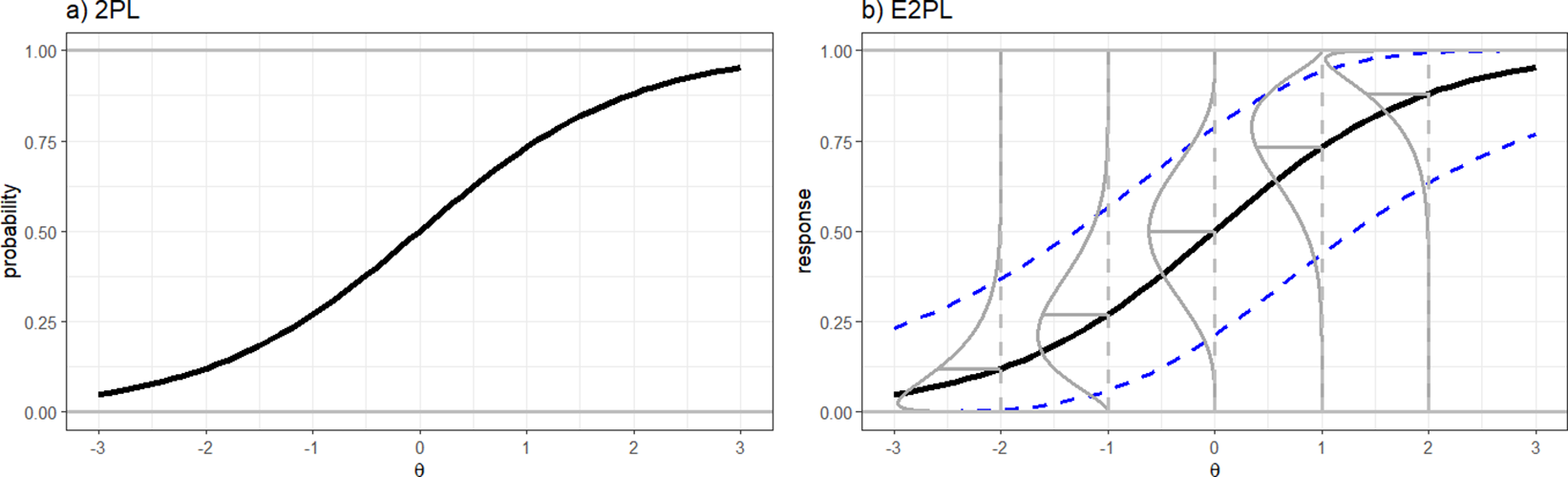


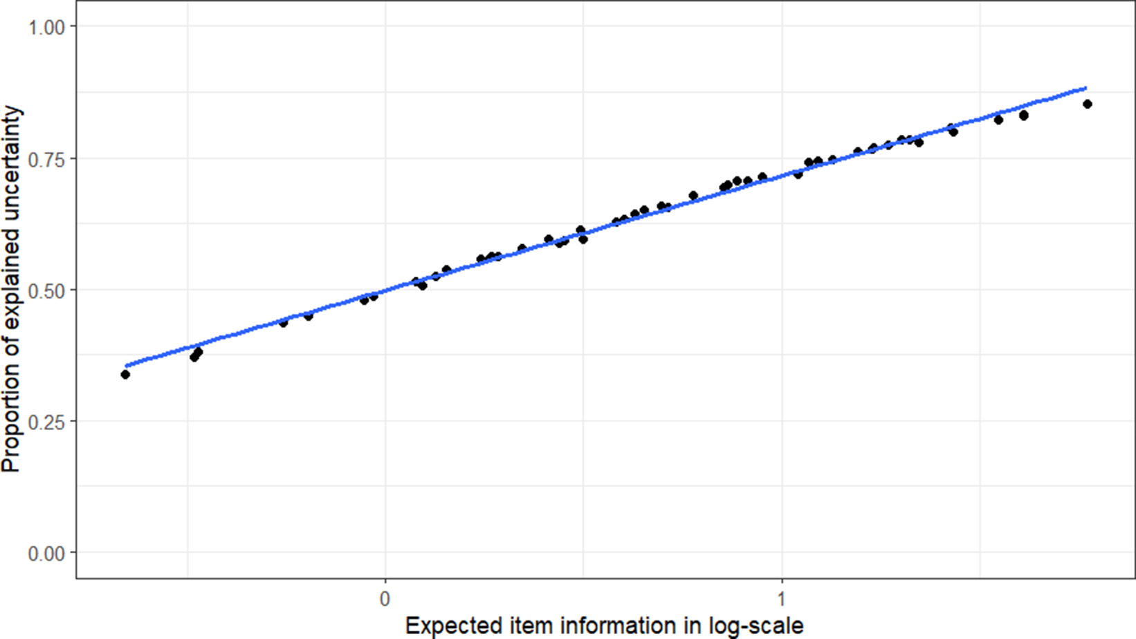


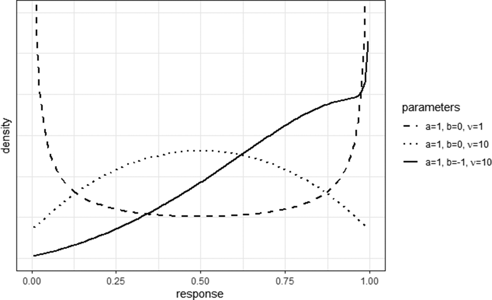


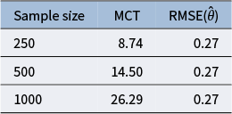


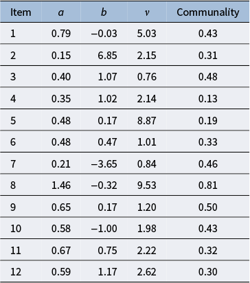


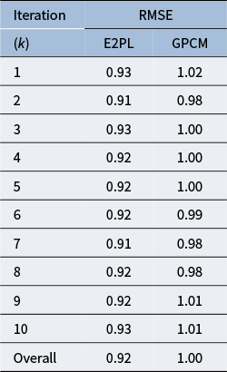

 Open access