


1 Introduction
One of the core challenges in creating a reliable radiocarbon (14C) calibration curve is ensuring that the statistical approach used for the curve’s production is able to accurately synthesize the various datasets which make up the curve, specifically recognizing and incorporating their diverse and unique aspects in doing so. This is particularly critical in light of the recent increase in the availability of high-precision radiocarbon determinations, and the consequent demand by users for ever more precise and accurate calibration. For IntCal20, not only is the underlying data available for use in curve construction considerably more numerous and detailed than in previous curves but, due to the advances in our wider understanding of the Earth’s systems, our insight into the specific and individual characteristics of much of that data has also improved. If we are able to harness and more accurately represent these specific features within our curve construction then this will hopefully improve the resultant calibration. To achieve this, for the new calibration curve we have completely revised the statistical methodology from a random walk to a Bayesian spline based approach. This new approach allows us to take better advantage of the underlying data and also to provide output which is more useful and relevant for calibration users.
Over the years, the IntCal statistical methodology has developed and improved alongside our understanding of the constituent data and as we gain more knowledge of the underlying Earth Systems processes. For IntCal98 (Stuiver et al. Reference Stuiver, Reimer, Bard, Beck, Burr, Hughen, Kromer, McCormac, van der Plicht and Spurk1998), the curve was produced via a combination of linear interpolation of windowed tree-ring averages and frequentist splines. In 2004, the approach was updated to a random walk model (Buck and Blackwell Reference Buck and Blackwell2004) which introduced an approximate Bayesian method, and began to incorporate some of the important additional aspects of the constituent data such as potential uncertainty in the calendar ages for the older determinations, and that many tree-ring observations related to multiple years of metabolization. This random walk was developed further for IntCal09 (Blackwell and Buck Reference Blackwell and Buck2008; Heaton et al. Reference Heaton, Blackwell and Buck2009) and IntCal13 (Niu et al. Reference Niu, Heaton, Blackwell and Buck2013) into a fully Bayesian MCMC approach that enabled the inclusion of more of the unique structures in the calibration datasets such as floating sequences of tree rings and more complex covariances in the calendar age estimates provided by wiggle-matching or palaeoclimate tie-pointing.
The random walk approach however had several disadvantages. While in principle, it allowed for modeling flexibility, the details of the implementation required a very large number of parameters that, despite being highly dependent, were predominantly updated individually. This made it extremely slow to run; difficult to ensure it explored the full space of possible curves; and also hard to assess whether the MCMC had reached its equilibrium distribution. Furthermore, this restricted the ability to explore the impact of specific modeling assumptions or individual data on the final curve. As the volume of the data used to generate IntCal has increased, alongside the need for further bespoke modeling of key data structures, this random walk approach to curve creation has consequently become computationally impractical for further use.
For the updated IntCal20 curve, the IntCal working group therefore requested a new approach to curve creation be developed. This new approach needed to be equally rigorous, from a statistical perspective, as the previous methodology; to incorporate the advances in both geoscientific understanding and radiocarbon precision that have occurred since 2013; and yet overcome the implementational difficulties of the previous random walk approach. Specifically, to increase confidence in the curve’s robustness and reliability the new approach needed to run at a speed which allowed investigation of the effect of key modeling choices not possible with the previous methodology. The new approach is based upon Bayesian splines with errors-in-variables as introduced by Berry et al. (Reference Berry, Carroll and Ruppert2002) but requires multiple bespoke innovations to accurately adapt to the specific data complexities. We believe it offers a significant improvement over previous approaches not just in the modeling but also the additional output it can provide for both calibration users and geoscientific users more widely.
The paper is set out as follows. In Section 2 we list the main advances made in the statistical methodology, data understanding and modeling since the last set of IntCal curves (Reimer et al. Reference Reimer, Bard, Bayliss, Beck, Blackwell, Bronk Ramsey, Buck, Cheng, Edwards, Friedrich, Grootes, Guilderson, Haflidason, Hajdas, Hatté, Heaton, Hoffmann, Hogg, Hughen, Kaiser, Kromer, Manning, Niu, Reimer, Richards, Scott, Southon, Staff, Turney and van der Plicht2013; Hogg et al. Reference Hogg, Hua, Blackwell, Niu, Buck, Guilderson, Heaton, Palmer, Reimer, Reimer, Turney and Zimmerman2013). We then provide, in Section 3, a short non-technical introduction to three key practical ideas for calibration users: an explanation of Bayesian splines; the importance of recognizing potential calendar age uncertainty in curve construction; and the modeling of potential over-dispersion in the data. Section 4 then describes the main technical details of curve construction. The IntCal20 curve is created in two sections with somewhat different statistical concerns. The more recent part of the curve, back to approximately 14 cal kBP, is based entirely upon tree-ring determinations, that are predominantly dendrodated with exact, known calendar ages. Here the main challenges are to incorporate the large amount of data, provide high resolution in the curve with appropriate uncertainties, and accurately incorporate blocked determinations that represent the measurement of multiple years. This is described in Section 4.3. Further back in time, the curve is based upon a wider range of 14C material where, as well as tree rings, we use direct and indirect records of atmospheric 14C in the form of corals, macrofossils, forams and speleothems. We describe the modifications required to incorporate these kinds of data in Section 4.4. This being a Bayesian approach we are able to incorporate prior information into our model and also provide posterior information on particular outputs of independent interest. In Section 5 we provide an indication of the kind of additional output the new methodology is able to provide. In particular the new approach generates not only pointwise means and variances for the calibration curve but, for the first time, sets of complete posterior realizations from 0–55 cal kBP which also allow access to covariance information. This covariance has the potential to improve future calibration of multiple radiocarbon determinations, for example in wiggle matches or more complex modeling. We also gain information on the level of additional variation (beyond laboratory reported uncertainty) present in tree-ring 14C determinations arising from the same calendar year. Finally, we discuss potential future work in Section 6 along with areas we have identified for further improvement for the next IntCal iteration. Note that the statistical approaches to the creation of SHCal20 (Hogg et al. Reference Hogg, Heaton, Hua, Palmer, Turney, Southon, Bayliss, Blackwell, Boswijk, Bronk Ramsey, Pearson, Petchey, Reimer, Reimer and Wacker2020 in this issue) and Marine20 (Heaton et al. Reference Heaton, Köhler, Butzin, Bard, Reimer, Austin, Bronk Ramsey, Grootes, Hughen, Kromer, Reimer, Adkins, Burke, Cook, Olsen and Skinner2020 in this issue) are presented within those papers and not discussed in detail here.
Notation
All ages in this paper and the database are reported relative to mid-1950 AD (= 0 BP, before present). Conventional, pre-calibration, 14C ages are given in units “ $^{\it14}{\it{C}}$yrs BP.” Calendar, or calibrated, ages are denoted as “cal BP” or “cal kBP” (thousands of calibrated years before present).
Data and Code
As in previous updates to the curve, the constituent data is available from the IntCal database http://www.intcal.org/. Other inputs are available on request, for example covariance matrices for the calendar ages of the tie-pointed records of the Cariaco Basin (Hughen and Heaton Reference Hughen and Heaton2020 in this issue), Pakistan and Iberian margin (Bard et al. Reference Bard, Ménot, Rostek, Licari, Böning, Edwards, Cheng, Wang and Heaton2013); and Lake Suigetsu (Bronk Ramsey et al. Reference Bronk Ramsey, Heaton, Schlolaut, Staff, Bryant, Brauer, Lamb, Marshall and Nakagawa2020 in this issue). Coding was performed in R (R Core Team 2019), using the fda (Ramsay et al. Reference Ramsay, Wickham, Graves and Hooker2018), mvtnorm (Genz et al. Reference Genz, Bretz, Miwa, Mi, Leisch, Scheipl and Hothorn2019), mvnfast (Fasiolo Reference Fasiolo2016) and Matrix (Bates and Maechler Reference Bates and Maechler2019) packages to efficiently create and fit the spline bases; and doParallel (Corporation and Weston Reference Corporation and Weston2019) to implement parallelization for the MCMC tempering. This code is available on request from the first author.
2 Developments in the IntCal20 statistical methodology
The main differences/improvements in the updated IntCal20 methodology over the previous random walk can be split into three broad categories: those relating to improvements in the statistical implementation itself; progress in the detailed modeling of unique data aspects that are enabled by the updated methodology; and finally, advances in the curve output that are both relevant to users of the calibration curve and of potential interest in their own right.
Improvements in Statistical Implementation
1. Bayesian Splines—the change from the random walk of Niu et al. (Reference Niu, Heaton, Blackwell and Buck2013) to splines allows a much more computationally feasible fitting algorithm. We retain the Bayesian aspect since it allows us to incorporate the various unique aspects of the calibration data; provides useful posterior information, e.g. the posterior calendar ages of the constituent data; and maintains consistency with calibration itself which is now universally implemented under that paradigm. This Bayesian spline approach is equally conceptually rigorous as the random walk but considerably more flexible and can be run much more quickly.
2. Change in modeling and fitting domain—function estimation via splines is based on a trade-off between creating a curve that passes close to the observed data yet is not too rough. Previously all aspects of the curve’s construction occurred in the radiocarbon age domain. However, this is not the natural space in which to either model the curve roughness or decide on fidelity of the data to the curve. In the older section of the 14C record, the measurement uncertainties on the radiocarbon age scale become non-symmetric. This causes difficulties in fairly assessing the fit of a model to observed data if we judge it in this radiocarbon age domain. Instead, it is more natural to assess model fit in F 14C where measurement uncertainty remains symmetric. Similarly, a more natural domain in which to model the curve roughness is in Δ 14C space. We therefore change our modeling domain to ${\Delta ^{14}}{\rm{C}}$ and our fitting domain to ${F^{14}}{\rm{C}}$ when creating the curve. See Section 3.1.2 for definitions of the radiocarbon age, ${F^{14}}{\rm{C}}$ and ${\Delta ^{14}}{\rm{C}}$ domains.
3. Over-dispersion in dendrodated trees—as the volume of data entering IntCal increases, it is key to make sure we do not produce a curve which is over-precise as this would give inaccurate calibration for a user. While laboratories attempt to quantify all
$^{\rm14}{\rm{C}}$ uncertainty in their measurements, including through intercomparison exercises such as Scott et al. (Reference Scott, Naysmith and Cook2017), there remain some sources of additional $^{\rm14}{\rm{C}}$ variation which are difficult for any laboratory to capture. For tree rings, potential examples include variation between local region, species, or growing season. Consequently, when we bring together $^{\rm14}{\rm{C}}$ measurements from the same calendar year, they may potentially be over-dispersed, i.e. more widely spread than would be expected given their laboratory quoted uncertainty. The new approach incorporates a term allowing for potential over-dispersion within 14C determinations of the tree rings so that, if additional variability is seen in the underlying IntCal data, the method will account for it and prevent excessive confidence in the resultant curve.4. Heavy tailed errors—in the older portion of the curve, where data come from a range of different
$^{\rm14}{\rm{C}}$ reservoirs, we aim to reduce the influence of potential outliers by permitting each dataset to have heavier tailed errors. These tails are adaptively estimated during curve construction.5. Improved model mixing and parallel tempering—when using any MCMC method, it is crucial to ensure that the chain has reached its equilibrium distribution and that it is not stuck in one part of the model space. This was a significant concern with the previous random walk approach since the curve was updated one calendar year at a time. Conversely, Bayesian splines enable updates of the complete curve simultaneously via Gibbs sampling. To address any additional concerns about mixing of the new MCMC and to ensure we explore the space of possible curves more freely, we also implement parallel tempering whereby we run multiple modified/tempered chains simultaneously in such a way that some can move around the space more easily. By appropriate switching between these tempered chains we can further improve model mixing.


Improvements in Data Modeling
These steps forward in the statistical implementation, while still maintaining computational feasibility, also enable us both to incorporate new data structures and to advance our modeling of the processes from which the data arise:
1. Large increase in volume of data throughout the curve—the new IntCal20 is based upon a much greater number of
$^{\rm14}{\rm{C}}$ determinations. These include many annual tree-ring determinations such as remeasurement within various laboratories of data from the period of Thera (e.g. Pearson et al. Reference Pearson, Brewer, Brown, Heaton, Hodgins, Jull, Lange and Salzer2018); new wiggle-matched and floating sequences of late-glacial tree rings (e.g. Capano et al. Reference Capano, Miramont, Shindo, Guibal, Marschal, Kromer, Tuna and Bard2020 in this issue); and new measurements of Hulu Cave extending further back in time (Cheng et al. Reference Cheng, Edwards, Southon, Matsumoto, Feinberg, Sinha, Zhou, Li, Li, Xu, Chen, Tan, Wang, Wang and Ning2018). In total, the new IntCal20 curve is based upon 12,904 raw 14C measurements compared to the 7019 used for IntCal13 (Reimer et al. Reference Reimer, Bard, Bayliss, Beck, Blackwell, Bronk Ramsey, Buck, Cheng, Edwards, Friedrich, Grootes, Guilderson, Haflidason, Hajdas, Hatté, Heaton, Hoffmann, Hogg, Hughen, Kaiser, Kromer, Manning, Niu, Reimer, Richards, Scott, Southon, Staff, Turney and van der Plicht2013). This rapid increase means a faster curve construction method is essential.2. Blocking in dendrodated trees—with the new radiocarbon revolution providing an increased ability to measure annual tree rings, there has been a concern that the inclusion within IntCal of determinations relating to decadal or bi-decadal averages alongside these new annual measurements could mean we lose critical information on short-term variation in atmospheric radiocarbon levels. Our approach fully recognizes the number of years each determination represents, meaning there is no loss of information as a result of such blocked determinations.
3. Variable marine reservoir ages—IntCal09 (Reimer et al. Reference Reimer, Baillie, Bard, Bayliss, Beck, Blackwell, Bronk Ramsey, Buck, Burr, Edwards, Friedrich, Grootes, Guilderson, Hajdas, Heaton, Hogg, Hughen, Kaiser, Kromer, McCormac, Manning, Reimer, Richards, Southon, Talamo, Turney, van der Plicht and Weyhenmeyer2009) and IntCal13 (Reimer et al. Reference Reimer, Bard, Bayliss, Beck, Blackwell, Bronk Ramsey, Buck, Cheng, Edwards, Friedrich, Grootes, Guilderson, Haflidason, Hajdas, Hatté, Heaton, Hoffmann, Hogg, Hughen, Kaiser, Kromer, Manning, Niu, Reimer, Richards, Scott, Southon, Staff, Turney and van der Plicht2013) modeled marine reservoir ages beyond the Holocene as constant over time. For IntCal20, we incorporate time-varying marine reservoir ages using the LSG model of Butzin et al. (Reference Butzin, Heaton, Köhler and Lohmann2020 in this issue) and a separate adaptive spline for the Cariaco Basin.
4. Inclusion of new floating tree-ring sequences—the new curve includes several new late-glacial trees which have calendar age estimates obtained via wiggle matching (Reinig et al. Reference Reinig, Nievergelt, Esper, Friedrich, Helle, Hellmann, Kromer, Morganti, Pauly, Sookdeo, Tegel, Treydte, Verstege, Wacker and Büntgen2018; Capano et al. Reference Capano, Miramont, Shindo, Guibal, Marschal, Kromer, Tuna and Bard2020 in this issue), as well as three entirely floating tree chronologies around the time of the Bølling-AllerødFootnote 1 (Adolphi et al. Reference Adolphi, Muscheler, Friedrich, Güttler, Wacker, Talamo and Kromer2017) and two older Southern Hemisphere floating kauri tree-ring sequences (Turney et al. Reference Turney, Fifield, Hogg, Palmer, Hughen, Baillie, Galbraith, Ogden, Lorrey and Tims2010, Reference Turney, Jones, Phipps, Thomas, Hogg, Kershaw, Fogwill, Palmer, Bronk Ramsey and Adolphi2017) on which we have no absolute dating information and which need to be placed accurately amongst the other data.
5. Rapid
$^{\rm14}{\rm{C}}$ excursions—there are several specific times when the level of atmospheric $^{\rm14}{\rm{C}}$ is known to vary extremely rapidly. For IntCal20 we have identified three such events around 774–5 AD, 993–4 AD and $\sim$660 BC (Miyake et al. Reference Miyake, Nagaya, Masuda and Nakamura2012, Reference Miyake, Masuda and Nakamura2013; O’Hare et al. Reference O’Hare, Mekhaldi, Adolphi, Raisbeck, Aldahan, Anderberg, Beer, Christl, Fahrni, Synal, Park, Possnert, Southon, Bard and Muscheler2019). Such rapid 14C changes will typically not be modeled well by standard regression which will tend to smooth them out. However, by increasing the density of knots forming our spline basis in the vicinity of these rapid excursions we can better represent these significant features.


Improvements in Output
The statistical innovations also mean that we can now provide several new facets to our output:
1. Annualized output—we are able to provide curve estimates on an annual grid enabling more detailed calibration. This will be needed in light of the increased demand to calibrate annual radiocarbon determinations. While we do not discuss the implications for calibration itself in this paper, such a detailed annual calibration curve will likely increase the potential for multimodal calendar age estimates which require significant care in interpretation, especially during periods of plateaus in the calibration curve. See the IntCal20 companion paper (van der Plicht et al. Reference van der Plicht, Bronk Ramsey, Heaton, Scott and Talamo2020 in this issue) for more details and an illustrative example with the calibration of the Minoan Santorini/Thera eruption.
2. Predictive intervals—if the IntCal20
$^{\rm14}{\rm{C}}$ data contain additional sources of variation beyond their laboratory quantified uncertainties (due to potential regional, species or growing season differences), i.e. they appear more widely spread around the calibration curve than can be explained by their quoted uncertainties, we will need to take this into account for calibration of new determinations too. Specifically, any $^{\rm14}{\rm{C}}$ determination a user calibrates against the curve is likely to contain similar levels of unseen additional variation. If we can assess the level of additional variation seen within the IntCal20 data, then we can incorporate this into calibration for a user by providing a predictive interval on the curve. Intuitively this predictive interval aims to incorporate both uncertainty in the value of the curve itself and potential additional uncertainty sources such as regional, species or growing season effects beyond the laboratory quoted uncertainty. These predictive intervals are therefore more relevant for calibration than curve intervals which do not incorporate or adapt to potential additional sources of variability.3. Posterior information arising from curve construction—the Bayesian implementation allows us to provide posterior estimates for many aspects of interest. For example, all of the records with uncertainties in their calendar timescales (the various floating tree-ring sequences, marine sediments, Lake Suigetsu and the speleothems) will be calibrated during the curve’s construction. We can provide these posterior calibrated age estimates along with other information such as the level of over-dispersion seen in the data, and posterior estimates of marine reservoir ages and dead carbon fractions.
4. Complete realizations of the curve from 0–55 cal kBP—historically IntCal output has consisted of pointwise posterior means and variances. However, the Bayesian approach provides a set of underlying curve realizations which provide covariance information on the value of the curve at any two calendar ages. When calibrating single determinations, this covariance does not affect the calendar age estimates obtained, i.e. calibrating against the pointwise posterior means and variances provides the same inference as calibrating against the set of individual curve realizations. However, when calibrating multiple determinations simultaneously, for example if we are seeking to determine the length of time elapsed between two determinations or fit a more complex model, use of these complete realizations in consequent calibration offers potential to improve insight. Work is planned by the group to explore how this may be best incorporated into existing calibration software.


We discuss some of these aspects in more detail, and present some of the output available, in Section 5 and the Supplementary Information.
3 A Brief Summary of Bayesian Splines, Errors-in-Variables and Predictive Intervals
For a typical calibration user the key elements of the new methodology consist of the change to Bayesian splines with the accompanying shift in the modeling and fitting domains; the continued recognition that many of the data have uncertainties in their calendar ages and the significant effect that has on curve estimation; and the use of predictive intervals on the published curve for calibration. We therefore commence with an intuitive explanation of these three elements. The technical details can be found later in Section 4. We note that, in our intuitive descriptions, the observational model may be further complicated by 14C determinations representing multiple, as opposed to single, calendar years and the inclusion of a reservoir age or dead carbon fraction for those observations which are not directly atmospheric. However, for clarity of exposition, we do not consider either of these factors here, and refer to Section 4 for details on how these additions can be incorporated.
3.1 Bayesian Splines and Choice of Modeling Domain
3.1.1 Frequentist Ideas
Suppose that we observe a function  $f$, subject to noise, at a series of times ${\theta _i}$, $i = 1, \ldots ,n$,
 $${Y_i} = f({\theta _i}) + {\varepsilon _i}\quad i = 1, \ldots ,n,$$
where, for the time being, we assume that the times  ${\theta _i}$ are known absolutely. To obtain a spline estimate for the unknown function we seek to find a function that provides a satisfactory compromise between going close to the data but yet does not overfit. This can be done by choosing the estimate $\hat f$ that minimizes, over a suitable set of functions,
 $$S(\,f) = {\texttt{FIT}}(\,f,Y) + \lambda {\texttt{PEN}}(\,f),$$
where  ${\texttt{FIT}}(\,f,Y)$ measures the lack of agreement between a potential $f$ and the observed $Y$; and ${\texttt{PEN}}(\,f)$ represents a penalty for functions that might be overfitting. Typically, ${\texttt{FIT}}(\,f,Y)$ consists of the sum-of-squares difference between $f({\theta _i})$ and ${Y_i}$, while ${\texttt{PEN}}(\,f)$ assesses the roughness of a proposed $f$ ensuring that the more variable f the larger the penalty given to it with the aim of preventing the spline estimate from overfitting the data. The parameter $\lambda$ determines the relative trade-off between how one values fidelity to the observed data, i.e. ${\texttt{FIT}}(\,f,Y)$, compared with function roughness, ${\texttt{PEN}}(\,f)$. A large $\lambda$ will heavily penalize roughness and typically results in a smooth curve that is less close to the data; while a small $\lambda$ will mean the spline goes closer to the data but at the expense of being more variable.
3.1.2 Selection of Appropriate Fitting and Modeling Domains for Radiocarbon
Within the radiocarbon community there are three commonly used domainsFootnote 2:  ${\Delta ^{14}}{\rm{C}}$, ${F^{14}}{\rm{C}}$ and the radiocarbon age. Given $g(\theta )$, the historical level of ${\Delta ^{14}}{\rm{C}}$ in year $\theta$ cal BP, we can freely convert between the domains as follows:
- ${F^{14}}{\rm{C}}$ domain: $f(\theta ) = \left( {{1 \over {1000}}g(\theta ) + 1} \right){e^{ - \theta /8267}}.$ The value of ${F^{14}}{\rm{C}}$, or fraction modern (Reimer et al. Reference Reimer, Brown and Reimer2004b), denotes the relative proportion of radiocarbon to stable carbon in a sample compared to that of a sample with a conventional radiocarbon age of 0 14C yrs BP (i.e. mid-1950 AD) after accounting for isotopic fractionation. It is a largely linear calculation from the instrumental measurements meaning its uncertainties are approximately normal.
Radiocarbon age domain:
$h(\theta ) = - 8033\ln f(\theta ).$ The radiocarbon age, in 14C yrs BP, is obtained from the fraction modern using Libby’s original half-life and without any calibration. Since this is a non-linear mapping of ${F^{14}}{\rm{C}}$, the uncertainties are no longer even approximately normally distributed as we approach the limit of the technique.


When fitting a smoothing spline, we have some flexibility in the precise choice of  ${\texttt{FIT}}(\,f,Y)$, our assessment of fit, and our roughness penalty ${\texttt{PEN}}(\,f)$. For radiocarbon purposes, the natural domain to assess the quality of fit of a proposed calibration curve to observations is the ${F^{14}}{\rm{C}}$ domain, the raw scale on which the determinations are obtained. In this ${F^{14}}{\rm{C}}$ domain, our measurement uncertainties are symmetric. Conversely, in the radiocarbon age domain these uncertainties become asymmetric as we progress back in time. We therefore choose
 $${\texttt{FIT(\,f,F)}} = \sum\limits_{i = 1}^n {1 \over {\sigma _i^2}}{\left(\, {f({\theta _i}) - {F_i}} \right)^2},$$
where  ${F_i}$ are the observed F 14C values of the determinations and ${\sigma _i}$ their associated uncertainties in the ${F^{14}}{\rm{C}}$ domain. ${F^{14}}{\rm{C}}$ is not however the most appropriate domain in which to assess roughness since it exhibits exponential decay over time making equitable penalization of potential calibration curves more difficult. Instead a more natural choice is the ${\Delta ^{14}}{\rm{C}}$ domain where, a priori, one might expect a calibration curve to display approximately equal roughness over its length. For our penalty function we therefore choose
 $${\texttt{PEN}}(\,f) = \int {\left\{ {g''(\theta )} \right\}^2}d\theta,$$
where  $g''(\theta )$ is the second derivative of the proposed level of ${\Delta ^{14}}{\rm{C}}$, a standard penalty for function roughness.
We summarize this by saying that we perform modeling in the Δ 14C domain as it is here we penalize roughness; while we perform fitting in the  ${F^{14}}{\rm{C}}$ domain since it is here we assess fidelity of the curve to the raw observations. Since, given $\theta$, the transformation from ${F^{14}}{\rm{C}}$ to ${\Delta ^{14}}{\rm{C}}$ is affine we can utilize these different modeling and fitting domains while still maintaining a practical spline estimation approach.
3.1.3 Bayesian Reframing
To reinterpret the above idea in a Bayesian framework we can split our functional
 $$S(\,f) = \sum\limits_{i = 1}^n {1 \over {\sigma _i^2}}{\left(\, {f({\theta _i}) - {F_i}} \right)^2} + \int {\left\{ {g''(\theta )} \right\}^2}d\theta$$
into two distinct parts. The penalty component  $\int {\left\{ {g''(\theta )} \right\}^2}d\theta$ can be considered as specifying the prior distribution on the space of calibration curves; more precisely, it gives the negative log density of the prior. Intuitively this summarizes our prior beliefs about the form of the calibration curve before we observe any actual data. We then wish to update this prior belief, in light of the observed data, to obtain our posterior. This updating is achieved via the fitting component $\sum\nolimits_{i = 1}^n {1 \over {\sigma _i^2}}{\left(\, {f({\theta _i}) - {F_i}} \right)^2}$ which represents the negative log-likelihood of the observed data under an assumption that each ${F_i} \sim N(\,f({\theta _i}),\sigma _i^2)$. The value of $S(\,f)$ then represents the negative posterior log-density for a potential calibration curve $f$.
$f$.
This idea is illustrated in Figure 1. In panel (a) we present three potential calibration curves in the  ${\Delta ^{14}}{\rm{C}}$ domain. Using just our prior, we give each curve an initial weight corresponding to their roughness. The black curve is the least rough and so would be given highest prior weight as a plausible potential calibration curve. The green curve is the roughest and so has least weight according to our prior. Each of these ${\Delta ^{14}}{\rm{C}}$ curves is then converted into the symmetric ${F^{14}}{\rm{C}}$ space and compared with our observations as shown in panel (b). The plausibility of each curve is then updated to incorporate the fit to this data. Based upon this, the red curve would have a higher posterior density as it fits relatively closely while not being overly rough. Both the green and black curves would have a low posterior density and so be considered highly implausible as they do not pass near the data. Use of MCMC allows us to generate any number of plausible calibration curves drawn from the posterior that provide a satisfactory trade-off between the roughness prior and fidelity to the observations. Some such realizations are shown in panels (c) and (d) in both the ${\Delta ^{14}}{\rm{C}}$ and ${F^{14}}{\rm{C}}$ domains respectively. These realizations are then summarized to produce the final IntCal20 curve.
An illustration of Bayesian splines. Panel (a) shows some potential calibration curves in the ${\Delta ^{14}}{\rm{C}}$ domain drawn from the prior. These are then compared with the observed data in the F 14C domain as shown in panel (b) to form our Bayesian posterior. The bottom two panels (c) and (d) show posterior realizations of potential curves (shown in Δ 14C and ${F^{14}}{\rm{C}}$ space respectively) obtained via MCMC that provide a satisfactory trade-off between agreement with our prior penalizing over-roughness and the fit to our observed data.

3.1.4 Variable Smoothing and Knot Selection
A further choice to be made when spline smoothing is the set of functions (or potential calibration curves) to search over for our functional  $S(\,f)$. This set is called a basis. We use cubic splines where this basis is determined by specifying what are known as knots at distinct calendar times. The more knots one has in a particular time period, the more the spline can vary. One common option, known as a smoothing spline, is to place a knot at every calendar age ${\theta _i}$ for $i = 1, \ldots ,n$. However, since we have a very large number of observations $n$ this is computationally impractical. Instead we use P-splines (see Berry et al. Reference Berry, Carroll and Ruppert2002, for details) where we select a smaller number of knots; this is equivalent to restricting the potential calibration curves to a somewhat smaller subspace of functions.
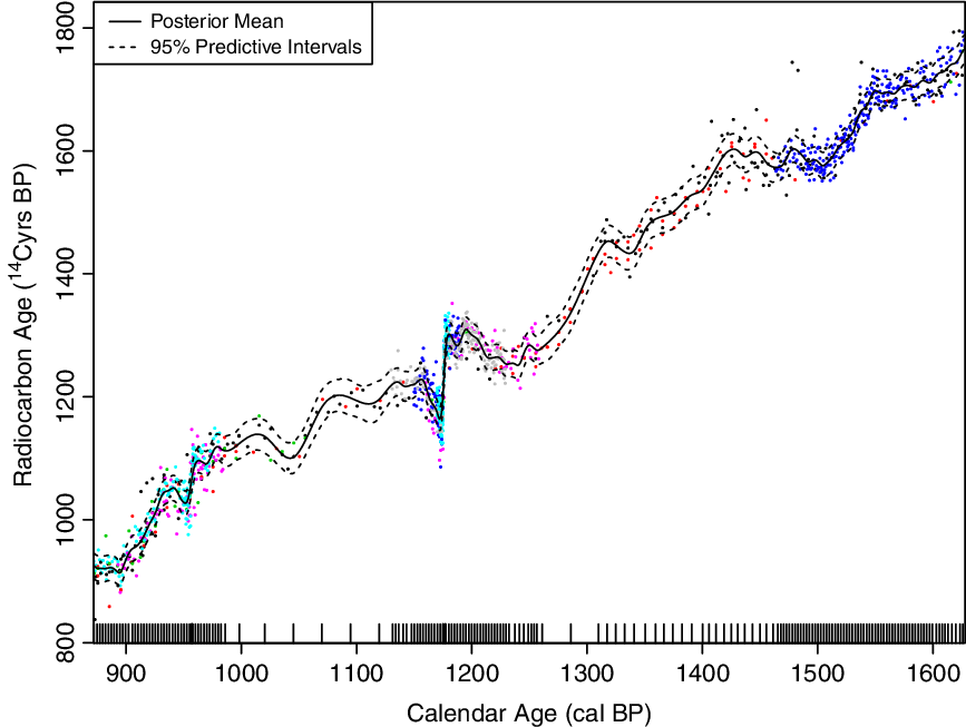
In implementing P-splines we need to make sure that the curves we consider are still able to provide sufficient detail for a calibration user and identify fine scale features such as solar cycles where we have the ability to do so. The data on which we base our curve have highly variable density. In some periods, such as recent dendrodated trees, we have a great density of determinations while in others the underlying data is more sparse. To adapt to this and keep required detail, we choose a large number of knots and place them at calendar age quantiles of the data to provide variable smoothing. This approach of locating the knots at observed quantiles is standard in the regression literature (e.g. Harrell Reference Harrell2001). Where our data is dense, we can pick out the required fine detail but where the data is more sparse we smooth more significantly. An example can be seen in Figure 2. This figure also highlights how we pack additional knots around known Miyake-type events, narrow spikes (sub-annual) of increased  $^{\rm14}{\rm{C}}$ production, to enable us to better retain these events in the final curve. For more details on choice of knots and placement see Sections 4.3.4 and 4.4.3.
Variable smoothing and knot selection. Shown as a rug of tick marks along the bottom are the locations of the knots for the cubic spline. These are placed at quantiles of the observed calendar ages to provide variable smoothing. In dense regions, we can identify more detail in the calibration curve; while where the underlying data is less dense we perform more smoothing. In particular, note the additional knots placed around the two Miyake-type events (i.e. 957 and 1176 cal BP) which allow the curve to vary much more rapidly at these times. The points from different datasets within the IntCal database are shown in different colors to distinguish them.
3.2 Errors-in-Variables Regression
3.2.1 Calendar Age Uncertainty
Within the IntCal database (http://www.intcal.org/), many of the determinations have calendar ages which are not known absolutely. This is particularly the case as we progress further back in time and calendar age estimates are constructed from uranium thorium (U-Th) dating, e.g. speleothems (Southon et al. Reference Southon, Noronha, Cheng, Edwards and Wang2012; Cheng et al. Reference Cheng, Edwards, Southon, Matsumoto, Feinberg, Sinha, Zhou, Li, Li, Xu, Chen, Tan, Wang, Wang and Ning2018; Beck et al. Reference Beck, Richards, Edwards, Silverman, Smart, Donahue, Hererra-Osterheld, Burr, Calsoyas, Jull and Biddulph2001; Hoffmann et al. Reference Hoffmann, Beck, Richards, Smart, Singarayer, Ketchmark and Hawkesworth2010) and corals (Bard et al. Reference Bard, Hamelin, Fairbanks and Zindler1990, Reference Bard, Arnold, Hamelin, Tisnerat-Laborde and Cabioch1998, Reference Bard, Ménot-Combes and Rostek2004; Cutler et al. Reference Cutler, Gray, Burr, Edwards, Taylor, Cabioch, Beck, Cheng and Moore2004; Durand et al. Reference Durand, Deschamps, Bard, Hamelin, Camoin, Thomas, Henderson, Yokoyama and Matsuzaki2013; Fairbanks et al. Reference Fairbanks, Mortlock, Chiu, Cao, Kaplan, Guilderson, Fairbanks, Bloom, Grootes and Nadeau2005; Edwards et al. Reference Edwards, Beck, Burr, Donahue, Chappell, Druffel and Taylor1993; Burr et al. Reference Burr, Beck, Taylor, Recy, Edwards, Cabioch, Correge, Donahue and O’Malley1998, Reference Burr, Galang, Taylor, Gallup, Edwards, Cutler and Quirk2004); varve counting, e.g. parts of Cariaco Basin (Hughen et al. Reference Hughen, Southon, Bertrand, Frantz and Zermeño2004) and Lake Suigetsu (Bronk Ramsey et al. Reference Bronk Ramsey, Heaton, Schlolaut, Staff, Bryant, Brauer, Lamb, Marshall and Nakagawa2020 in this issue); and palaeoclimate tuning/tie-pointing, e.g. other parts of Cariaco Basin (Hughen and Heaton Reference Hughen and Heaton2020 in this issue), and the Pakistan and Iberian Margins (Bard et al. Reference Bard, Ménot, Rostek, Licari, Böning, Edwards, Cheng, Wang and Heaton2013). Furthermore, in the case of several of the floating tree-ring sequences, we have only a relative set of calendar ages and no absolute age estimate. Regression in this situation is called errors-in-variables since we have errors/uncertainties in both the calendar age and radiocarbon determination variables. For these observations we therefore observe pairs  ${\left\{ {({F_i},{T_i})} \right\}_{i \in {\cal I}}}$ where:
 $$\eqalign{{F_i} = f({\theta _i}) + {\varepsilon _i}, \cr {T_i} = {\theta _i} + {\psi _i}.}$$
 Here  $f( \cdot )$ is our calibration curve of interest in the F 14C domain; ${\varepsilon _i} \sim N(0,\sigma _i^2)$ independently; and ${\psi _i}$ describes the uncertainty in our calendar age estimate. The form of this calendar age uncertainty varies between the datasets. While there is no restriction on the distribution of ${\psi _i}$ for our Bayesian spline approach, we model all these calendar age uncertainties as normally distributed but with appropriate covariances. For some sets they are considered independent, e.g. corals dated by U-Th; while for others, e.g. floating tree-ring sequences and those records dated by varve counting or palaeoclimate tie-pointing (Heaton et al. Reference Heaton, Bard and Hughen2013), there is considerable dependence between the observations. For more detail on the various covariance structures in the calendar age uncertainties see Niu et al. (Reference Niu, Heaton, Blackwell and Buck2013).
3.2.2 Importance of Recognizing Calendar Age Uncertainty
Incorporation of calendar age uncertainty in the construction of the IntCal calibration curves has occurred since IntCal04 (Reimer et al. Reference Reimer, Baillie, Bard, Bayliss, Beck, Bertrand, Blackwell, Buck, Burr, Cutler, Damon, Edwards, Fairbanks, Friedrich, Guilderson, Hogg, Hughen, Kromer, Manning, Bronk Ramsey, Reimer, Remmele, Southon, Stuiver, Talamo, Taylor, van der Plicht and Weyhenmeyer2004a) and is key for reliable curve construction. It was therefore crucial to retain within the new methodology. A range of statistical methods have been developed to deal with errors-in-variables regression. From the frequentist, non-Bayesian, perspective Fan and Truong (Reference Fan and Truong1993) introduced a kernel-based approach which achieves global consistency; Cook and Stefanski (Reference Cook and Stefanski1994) proposed a more general approach known as SIMEX. These approaches were not however considered suitable for our application due to the genuine prior information we have on certain aspects of the data; the wider, almost universal, use of Bayesian methodology within radiocarbon calibration; and the independent interest in several aspects of the calibration data which could be provided more simply through a Bayesian method. We therefore began the development of our method using the Bayesian splines of Berry et al. (Reference Berry, Carroll and Ruppert2002).
The effect of not recognizing calendar age uncertainty, where it is present, in regression is quite varied. In the case that the calendar age uncertainties are entirely independent of one another, such as U-Th dating, not recognizing calendar age uncertainty will typically result in curve estimates that are overly smooth and do not attain the peaks and troughs of the true underlying function. See Samworth and Poore (Reference Samworth and Poore2005) for an illustrative case study. However, in the case of IntCal, the situation is made more complicated by the shared dependence of the calendar age estimates within particular datasets. Specifically, the entire timescale for, e.g. Hulu Cave, is not the same as the Suigetsu or Cariaco timescale. As a consequence, all of these individual datasets may show the same overall features but at slightly different times. We require our method to recognize that these different timescales may need to be aligned, within their respective uncertainties, to keep these shared features. This requires us to shift multiple ages jointly by stretching/squashing the timescales accordingly. A failure to adapt to this joint calendar age uncertainty can give curve estimates which either introduce spurious wiggles as the curve flips between the different datasets or lose major features entirely.
Illustration
We provide in Figure 3 an illustrative example of the need to incorporate calendar age uncertainty. For simplicity, in this example, we fit and model our spline in the same domain. We consider a straightforward underlying function which we wish to reconstruct from 100 noisy observations  $\left\{ {({Y_i},{T_i})} \right\}_{i = 1}^{100}$
 $$f(\theta ) = {e^{ - \theta }}\sin (4\pi \theta ) + \cos (2\pi \theta )),$$
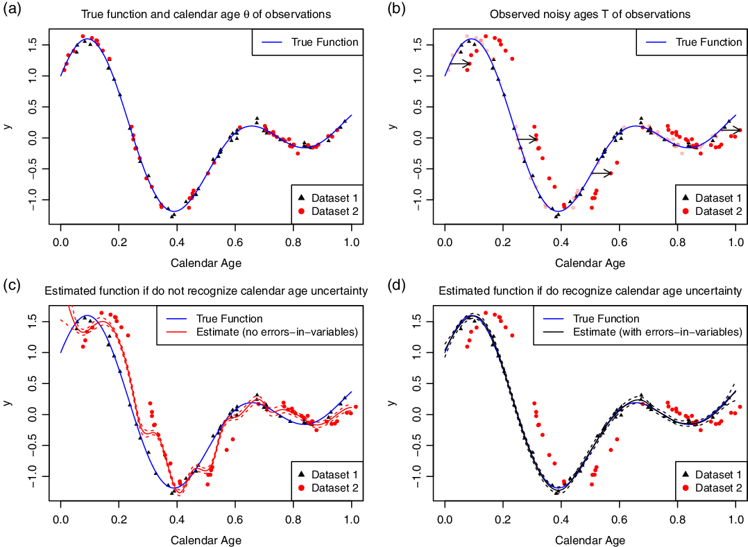
The importance of recognizing calendar age uncertainty (and correctly representing covariance within that uncertainty) when constructing a curve based on data arising from records with different observed timescales. Panel (a) shows the true, underlying, calendar ages of the data in two different records; while panel (b) shows a joint shift in the observed calendar ages within record 2. In such a case that observed timescales in two records are offset from one another, if we ignore this calendar age uncertainty then our spline estimate will introduce spurious variation as it flips between the records as in panel (c). Conversely if we incorporate such calendar age uncertainty and accurately represent it then we can still recover the underlying function accurately, as shown in (d).
where our underlying  ${\theta _i} \sim Beta(1.1,1.1)$ and observed ${Y_i} \sim N(\,f({\theta _i}{),0.05^2})$ for $i = 1, \ldots ,100$. Further, let us assume that these observations arise from two different sediment cores, 50 from core 1 (shown as black triangles) and 50 from core 2 (shown as red dots) as seen in panel (a). Within core 1, the calendar ages are known absolutely. However, within core 2 the observed timescale is somewhat shifted/biased so that when we observe the calendar ages $T$ in this core they all share the same joint shift from their true values, i.e.
 $${T_i} = {\theta _i}\,\,\,\,\,\,\,\,\,\,\,\,\,\,\,\,\,{\rm{if}}\;i\;{\rm{is\,in\,core\,1,}}$$
 $${T_i} = {\theta _i} + \psi\,\,\,\,\,\,{\rm{if}}\;i\;{\rm{is\,in\,core\,2,}}$$
where  $\psi \sim N{(0,0.1^2})$. The observed pairs $\left\{ {({Y_i},{T_i})} \right\}_{i = 1}^{100}$ are presented in panel (b) showing the shift in timescale within core 2. If we attempt to reconstruct the function using splines based upon our observed $\left\{ {({Y_i},{T_i})} \right\}_{i = 1}^{100}$ without recognizing the calendar age uncertainty, i.e. assuming both cores are on the same timescale, then we obtain the estimate in the panel (c). The estimate is spuriously variable as the spline will try to pass near all of the data on their non-comparable timescales. Conversely, if we recognize that the timescale in core 2 may need to be shifted onto the timescale of core 1, we obtain the estimate shown in panel (d). If we inform our Bayesian method that the calendar age observations in core 2 are subject to uncertainty, it will estimate the size of the joint shift needed to register core 2 onto the true timescale of core 1 and simultaneously reconstruct the true underlying function.
Implications for Visually Assessing Curve Fit
While it is important to incorporate errors-in-variables in curve construction, and accurately represent any dependence in the calendar age uncertainties, this does cause some difficulty in visually assessing the quality of fit between the raw constituent data and the final IntCal curve. Since the proposed method can shift the calendar ages of the observed data left and right within their uncertainties as described, one cannot estimate the final curve’s goodness-of-fit by eye using only the radiocarbon age axis if the raw data are only plotted at their initial, observed calendar ages. The method will have tried to align shared features even if they occur at somewhat different observed times within the different sets. This should be taken into consideration when viewing the final curve against the raw data. We provide the posterior calendar age estimates for the true calendar ages  ${\theta _i}$ for all the data. The difficulty of assessing the fit of the curve by eye is further compounded by the offsets in $^{\rm14}{\rm{C}}$ described in Section 4.4, in particular the marine reservoir ages which vary significantly over time and so will change as the MCMC updates the calendar ages of the data.
3.3 Predictive Intervals and Over-Dispersion
3.3.1 Background and Motivation
As well as creating a curve which has the correct posterior mean, it is key to make sure we provide appropriate intervals on the curve to ensure that, when used for calibration, the calendar age estimates produced are not over- or under-precise. This becomes particularly relevant for IntCal20 due to the large increase in data available to create the curve, and also the increased measurement precision provided by current laboratories. In addition to the laboratory reported uncertainty, there are a wide range of possible further sources of variation in the recorded  $^{\rm14}{\rm{C}}$ within objects of the same age, for example determinations come from different locations; have different local environments; tree rings may be of different species; and have different periods of growth due to local weather and so may have differing elements of wood from late/early growth. Even when the same sample is measured in different laboratories, we have evidence of a greater level of observation spread (i.e. over-dispersion) in the $^{\rm14}{\rm{C}}$ measurements within objects from the same calendar year than the laboratory reported uncertainties would support (see e.g. Scott et al. Reference Scott, Naysmith and Cook2017). Recognizing this potential over-dispersion, whatever its cause, is important both for curve estimation and resultant calibration for IntCal20. Specifically, if there is more variation in determinations from the same calendar year than the uncertainties reported by the laboratory, we need to make sure we incorporate that in our modeling, and also recognize its existence in the objects users will then calibrate against the IntCal20 curve.
We achieve this through the inclusion of a term to quantify the level of over-dispersion which we adaptively estimate, based on the high-quality and dense IntCal data, within our curve construction. This ensures that our IntCal20 curve does not become over-precise as an estimate of the Northern Hemispheric average. However, this alone is not sufficient for calibration since any additional sources of variation seen within the IntCal data are also likely to be present in uncalibrated determinations. We must therefore propagate this over-dispersion through to the calibration process itself. This is achieved using predictive curve intervals which incorporate not only uncertainty in the Northern Hemispheric average atmospheric curve but also the potential additional sources of variation seen in individual  $^{\rm14}{\rm{C}}$ determinations. Importantly, if no such additional variability exists then our model will estimate this appropriately, however if such additional sources of variability do seem present in the calibration data, our method will also recognize this and adapt accordingly. Without such an over-dispersion term then, as we get more data, the calibration curve will have intervals that become narrower and narrower even if the underlying data suggests considerably higher variability. Eventually, this would mean that the data entering the curve itself would potentially not calibrate to their known ages.
Such an idea of irreducible uncertainty was introduced in Niu et al. (Reference Niu, Heaton, Blackwell and Buck2013) but here we extend the idea further and generate predictive curve intervals which are more relevant for calibration users. Importantly, this does not however mean that we produce a calibration tool that any measurement (no matter its quality) can be calibrated against—we wish to maintain a calibration curve which has basic minima for data quality for both what goes into its construction and also what can be reliably calibrated using it.
3.3.2 The Over-Dispersion Model: Additive Errors Scaling with $\sqrt {{F^{14}}{\rm{C}}}$

The basic tree-ring model for an annual measurement assumes that a determination of calendar age  $\theta$ arises from a hemispherically uniform atmospheric level of $^{\rm14}{\rm{C}}$ shared by all determinations of the same calendar age. Under this model, the only uncertainty is that reported by the laboratory so that, in the F 14C domain, the observed value is
 $${F_i} = f({\theta _i}) + {\varepsilon _i},$$
where  ${\theta _i}$ is the year the determination represents; and ${\varepsilon _i} \sim N(0,\sigma _i^2)$ with ${\sigma _i}$ the uncertainty reported by the laboratory. The function $f(\theta )$ is our unique estimate of the hemispheric level of ${F^{14}}{\rm{C}}$ present in the atmosphere at calendar age $\theta$.
Currently it is not feasible to identify the specific sources that may potentially contribute extra variability beyond that reported by the laboratory (e.g. regional, species, growing season differences) and so we aim to cover them all in a unified approach. We therefore modify the above model to allow any determination to have an additional and independent source of potential variability  ${\eta _i}$ beyond that reported by the laboratory, i.e.
 $${F_i} = f({\theta _i}) + {\varepsilon _i} + {\eta _i}\quad {\rm{for}}\ i = 1, \ldots ,n$$
where  ${\eta _i} \sim N(0,\tau _i^2)$ are independent random effects with unknown variance $\tau _i^2$. To create the curve we simultaneously estimate both ${\tau _i}$, the level of over-dispersion, and the calibration curve $f( \cdot )$.
After investigation of several options, see Section 5.1 and the Supplementary Information, we model the level of over-dispersion (i.e. the level of any additional variability) to scale proportionally with the underlying value of  $\sqrt {f(\theta )}$ i.e. ${\tau _i} = \tau \sqrt {f({\theta _i})}$ so that ${\eta _i} \sim N(0,{\tau ^2}f(\theta ))$. We choose a prior for the constant of proportionality $\tau$ based upon data taken from the SIRI inter-comparison project (Scott et al. Reference Scott, Naysmith and Cook2017), and update this prior within curve construction based upon the IntCal data. The information provided by the very large volume of IntCal data dominates the SIRI prior and so the posterior estimate for the level of over-dispersion is primarily based upon the high-quality IntCal data.
3.3.3 Implications for Calibration
A user seeking to calibrate a high-quality 14C determination against the IntCal20 curve is likely to have a measurement that has been subject to similar additional sources of potential variation to whatever is seen in the IntCal data, and so have a similar level of over-dispersion. However, such a user typically has no way of assessing this over-dispersion themselves. Consequently, they should calibrate their determination using predictive curve estimates which additionally account for potential over-dispersion in their own determination. These predictive estimates are based upon the posterior of
 $$f(\theta ) + \eta (\theta ),$$
where  $\eta (\theta ) \sim N(0,{\tau ^2}f(\theta ))$ and $\tau$ is the posterior estimate of over-dispersion based upon the IntCal data. For IntCal20 we therefore report this predictive interval since it is more relevant for calibration. It is slightly wider than the corresponding credible interval for $f$ but more likely to give accurate calibrated dates.
Note that the level of over-dispersion, and hence the predictive intervals, we incorporate into the IntCal20 curve is based upon the high-quality, and screened, IntCal database. If a new uncalibrated  $^{\rm14}{\rm{C}}$ determination has additional sources of variability beyond those present in the IntCal tree-ring database (e.g. tree-ring species or locations not represented in IntCal, or a non-tree-ring sample) then this may mean that the level of over-dispersion for that uncalibrated determination is higher than that incorporated within the IntCal prediction intervals. This would result in a potentially over-precise calibrated age estimate. Users are advised to be cautious in such circumstances.
4 Creating the curve
As in previous versions of IntCal, the IntCal20 curve itself is created in two linked sections. Firstly we create the more recent part of the curve (extending from 0 cal kBP back to approximately 14 cal kBP) which is predominantly based upon dendrodated tree-ring determinations. Secondly we create the older part of the curve (from approximately 14 cal kBP back to 55 cal kBP) which is based upon a wider range of material, e.g. corals, macrofossils, forams, speleothems as well as five floating tree-ring chronologies, that are of uncertain calendar ages. Furthermore, these older  $^{\rm14}{\rm{C}}$ determinations are often not direct atmospheric measurements and hence have marine reservoir ages or dead carbon fractions. We therefore split our technical description of the approach accordingly. The two curve sections are stitched together to ensure smoothness and continuity through appropriate design of spline basis and conditioning the older part of the curve on the, already estimated, more recent section. This means that we can still produce sets of complete curve realizations from 0–55 cal kBP. Future work will aim to adapt the approach into a single step, updating the entire 0–55 cal kBP range as one.
4.1 Notation
Calibration Curve by Domain
We can represent the atmospheric history of  $^{\rm14}{\rm{C}}$, as a function of calendar age $\theta$, in three domains equivalently: ${\Delta ^{14}}{\rm{C}}$, ${F^{14}}{\rm{C}}$, and radiocarbon age. For any proposed history, i.e. calibration curve, we switch between these domains as appropriate within our statistical methodology. Let us denote:
- $g(\theta )$—the 14C calibration curve represented in Δ 14C space, i.e. the level of ${\Delta ^{14}}{\rm{C}}$ at $\theta$ cal BP. We model $g(\theta )$ in our spline basis and penalize roughness of the curve in this domain.
- $f(\theta )$—the $^{\rm14}{\rm{C}}$ calibration curve represented in ${F^{14}}{\rm{C}}$ space. Given $g(\theta )$ then$$f(\theta ) = \left( {{1 \over {1000}}g(\theta ) + 1} \right){e^{ - \theta /8267}}.$$
It is this
${F^{14}}{\rm{C}}$ domain that is used to assess goodness-of-fit to the observed data. •
$h(\theta )$—the $^{\rm14}{\rm{C}}$ calibration curve represented in radiocarbon age:$$h(\theta ) = - 8033\ln f(\theta ).$$This is the domain in which the calibration curve is plotted in the main IntCal20 paper (Reimer et al. Reference Reimer, Austin, Bard, Bayliss, Blackwell, Bronk Ramsey, Butzin, Cheng, Edwards, Friedrich, Grootes, Guilderson, Hajdas, Heaton, Hogg, Hughen, Kromer, Manning, Muscheler, Palmer, Pearson, van der Plicht, Reimer, Richards, Scott, Southon, Turney, Wacker, Adolphi, Büntgen, Capano, Fahrni, Fogtmann-Schulz, Friedrich, Köhler, Kudsk, Miyake, Olsen, Reinig, Sakamoto, Sookdeo and Talamo2020 in this issue).


Observed Data
We consider all of our observations in  ${F^{14}}{\rm{C}}$ since, as explained in Section 3.1, in this domain our 14C measurement uncertainties are symmetric. We define:
- ${F_i}$—the observed F 14C value of the data used to create the IntCal20 curve.
- ${\sigma _i}$—the laboratory-reported uncertainty on the observed ${F^{14}}{\rm{C}}$.
- ${m_i}$—the number of annual years of metabolization that a determination represents. The determination is considered to represent the mean of this block.
- ${T_i}$—the observed calendar age of a determination, which could either be the true calendar age (in the case of absolutely dendrodated determinations) or an estimate with uncertainty (in the case of e.g. corals, varves, speleothems).


Model Parameters
Within the model we update:
- ${\beta _j}$—the spline coefficients which describe the calibration curve.
- $\lambda$—the smoothing parameter for the spline estimate.
- ${\theta _i}$—the true calendar age of a determination or, in the case of a block-average determination, the most recent year of metabolization included in the block.
- $\tau$—the level of over-dispersion in the observed ${F^{14}}{\rm{C}}$ under a model whereby the potential additional variability for determination ${F_i}$ is ${\eta _i} \sim N(0,{\tau ^2}f({\theta _i}))$.
- ${r_{\cal K}}(\theta )$—the offset measured in terms of radiocarbon age, either due to dead carbon fraction (dcf) or marine reservoir age (MRA), between a determination from set ${\cal K}$ and the atmosphere at time $\theta$ cal BP. These will be specified either by ${\nu _{\cal K}}$, the mean dcf offset/coastal MRA shift for a particular dataset; or further spline coefficients ${\beta_{\rm{C}}}$ in the case of the Cariaco unvarved record. These are only needed when estimating the older part of the curve.
- ${\kappa _i}$ and ${\varrho _{\cal K}}$—adaptive error multipliers for data arising from the older time period to enable heavier tailed errors and the down-weighting of outliers. Also only included when estimating the older part of the curve.


4.2 Basic Model for Observed Data and Curve
As described in Section 3.1, we fit our curve to the data in the  ${F^{14}}{\rm{C}}$ domain while the curve modeling is performed in the ${\Delta ^{14}}{\rm{C}}$ domain. Specifically, for a single-year determination of the direct atmosphere with no offset and no over-dispersion, we observe pairs $({F_i},{T_i})_{i = 1}^n$ where
 $$\eqalign{{F_i} = f({\theta _i}) + {\varepsilon _i},\cr = \left( {{{g({\theta _i})} \over {1000}} + 1} \right){e^{ - \theta /8267}} + {\varepsilon _i}; \cr {T_i} = {\theta _i} + {\psi _i}.}$$
 Here  $g(\theta )$, the value of ${\Delta ^{14}}{\rm{C}}$ over time, is modeled as
 $$\eqalign{g(\theta ) = \sum\limits_{j = 1}^K {\beta _j}{B_j}(\theta )\cr = {\bi{B}}{(\theta )^T}{\bi{\beta}},}$$
where  ${\bi{B}}(\theta ) = ({B_1}(\theta ), \ldots ,{B_K}(\theta {))^T}$ and the ${B_j}( \cdot )$ are cubic B-splines (Green and Silverman Reference Green and Silverman1993) at a chosen fixed set of knots. To maintain computational feasibility, we consider $K \ll n$ so that the number of splines in our basis is considerably smaller than the total number of observations in the IntCal database. Knot number and placement is discussed in Sections 4.3.4 and 4.4.3.
Prior on $\bi{\beta}$

The Bayesian spline approach, equivalent to penalizing roughness in  ${\Delta ^{14}}{\rm{C}}$ by $\lambda \int_a^b {\left\{ {g''(\theta )} \right\}^2}d\theta$, is obtained by placing a “partially improper” Gaussian process on the spline coefficients β:
 $$\pi ({\bi{\beta}}|\lambda ) = {\left( {{\lambda \over {2\pi }}} \right)^{{\rm{rank}}({\bf{D}})/2}}{(|{\bf{D}}{|^ \star })^{1/2}}\exp \left\{ { - {\lambda \over 2}{{\bi{\beta}}^T}{\bf{D}}{\bi{\beta}}} \right\},$$
where  ${\bf{D}}$ is a penalty matrix which penalizes the integrated squared second derivative and $|{\bf{D}}{|^ \star }$ its generalized determinant (see Green and Silverman Reference Green and Silverman1993, for details). For splines of degree $m$ (cubic splines have degree 3) then ${\rm{rank}}({\bf{D}}) = K - (m - 1)$.
Prior on $\lambda$

As standard within Bayesian splines (e.g. Berry et al. Reference Berry, Carroll and Ruppert2002), we place a hyperprior on the smoothing parameter  $\lambda \sim Ga(A,B)$:
 $$\pi (\lambda ) = {1 \over {\Gamma (A){B^A}}}{\lambda ^{A - 1}}\exp \left( { - {\lambda \over B}} \right)\quad \quad {\rm{(for}}\ \lambda > 0).$$
 We select an uninformative prior on  $\lambda$ with $A = 1$ and $B = 50000$.
4.3 Creating the Predominantly Dendrodated Part of the Curve Back to Approximately 14 cal kBP
Back to approximately 14 cal kBP, we have a sufficient density of tree-ring determinations that we can estimate the curve based solely upon these direct atmospheric observationsFootnote 3. The main challenges in creating this more recent section of the curve are:
High density and volume of data—there are 10,713
$^{\rm14}{\rm{C}}$ measurements in this, predominantly dendrodated, section. Such a large volume of data makes a computationally efficient algorithm essential.Consequent demand for high level of detail in calibration curve—this, more recent, period of the calibration curve is the most heavily interrogated by archaeologists who require high precision, not just for individual calibration but also for modeling of multiple dates. This increases the user demand for fine detail in the calibration curve, e.g. incorporating solar cycles.
Blocking within the data—many of the
$^{\rm14}{\rm{C}}$ determinations do not relate to the measurement of the atmospheric $^{\rm14}{\rm{C}}$ in a single year but rather averages of multiple tree rings and so represent multiple years.Floating tree-ring sequences around
$12.7$ cal kBP—several late glacial trees have their chronologies estimated by wiggle matching and so while their internal chronology is known absolutely, their absolute ages are not. Otherwise, the true calendar ages of all determinations are known absolutely for this section of curve.


4.3.1 Modifications to Basic Model
Blocking and Additive Errors
Our model for the tree-ring determinations, taking account of blocking, considers the observed  ${F_i}$ as
 $${F_i} = {1 \over {{m_i}}}\left\{ {\sum\limits_{j=0}^{{m_i} - 1} f({\theta _i} + j)} \right\} + {\varepsilon _i} + {\eta _i}\quad {\rm{for}}\ i=1, \ldots ,n$$
 where  ${m_i}$ is the number of annual rings in the block for that determination; ${\theta _i}$ is the most recent year (start ring) of the block; and ${\varepsilon _i} \sim N(0,\sigma _i^2)$ where ${\sigma _i}$ is the uncertainty reported by the laboratory. This implicitly assumes that the tree rings over the section of ${m_i}$ rings are approximately equal in width, so that approximately equal annual amounts of wood were deposited and have ended up in the final measured sample. The ${\eta _i} \sim N(0,\tau _i^2)$ are independent random effects, with ${\tau _i}$ unknown, that represent potential over-dispersion in the $^{\rm14}{\rm{C}}$ determinations.
Additive Errors Model
As described in Section 5.1 we model  ${\tau _i}$, the standard deviation of the additive over-dispersion on the $i$th determination, as proportional to the square-root of the underlying ${F^{14}}{\rm{C}}$, i.e.
 $$\tau _i^2 = {\tau ^2}\ {1 \over {{m_i}}}\sum\limits_{j = 0}^{{m_i} - 1} f({\theta _i} + j).$$
 The individual values of  ${\eta _i}$ are not of interest and so we integrate them out, updating only the overall constant of proportionality $\tau$. Formally, a structure where ${\tau _i}$ depends upon the underlying curve means this term should be incorporated in the update to $\bi{\beta}$ within our sampler—a change to the curve (via its spline coefficients $\bi{\beta}$) would mean a change to the additive uncertainty ${\tau _i}$ on all observations. However, this would make the $\bi{\beta}$ update no longer a Gibbs step. Since, given the overall multiplier $\tau$, the change in ${\tau _i}$ between two potential curves is minimal, when updating $\bi{\beta}$ we consider ${\tau _i}$ as fixed; see Section 4.3.3 for more details.
Floating Tree-Ring Sequences
Several late-glacial tree sequences measured by Aix, ETH and Heidelberg (Reinig et al. Reference Reinig, Nievergelt, Esper, Friedrich, Helle, Hellmann, Kromer, Morganti, Pauly, Sookdeo, Tegel, Treydte, Verstege, Wacker and Büntgen2018; Capano et al. Reference Capano, Miramont, Shindo, Guibal, Marschal, Kromer, Tuna and Bard2020 in this issue) were dated by wiggle-matching so, while their internal relative chronologies were known precisely, their absolute calendar ages were somewhat uncertain. For such a floating tree-ring sequence, the true calendar ages are:
 $$\theta _j^{{\rm{float}}} = \xi + {\delta _j}\ {\rm{for}}\ j\ {\rm{in\ floating\ sequence}}.$$
 where  $\xi$ is the unknown start date (i.e. most recent year) of the floating sequence and ${\delta _j}$ is the precisely-known internal ring-count chronology. We place a discretized (integer) normal prior on $\xi \sim N(M,{N^2})$. Here, the prior mean $M$ and variance ${N^2}$ for the start date of each such tree-ring sequence were provided. All of the other dendrodated determinations were assumed to have their calendar age ${\theta _i}$ known absolutely.
4.3.2 Efficient Incorporation of Blocking
To incorporate blocking exactly, at each iteration of our MCMC we need to evaluate the level of  ${F^{14}}{\rm{C}}$ at every year represented within a block, and then average over them appropriately for each of our $n$ determinations. One might think this additional calculation will make the method much slower as it requires the evaluation of the curve at many more than n calendar years. However, in the predominantly dendrodated part of the curve, it is possible to exactly incorporate blocking without any compromise on the speed of the estimation procedure. Since the vast majority of the data in this period have exactly known calendar ages (only the floating tree-ring sequences have uncertain ages) we can calculate an initial matrix that relates, for each blocked determination, the necessary averaged ${F^{14}}{\rm{C}}$ to the underlying spline coefficients. This matrix then remains fixed throughout estimation. Further it has the same dimensions as if blocking had been ignored and hence does not significantly alter the speed of the MCMC updates.
Finding Values of ${\bi{F^{14}}{\bi{C}}}$ at Each Year Represented in a Block

We begin by describing how we can relate each blocked determination to the spline coefficients  $\bi{\beta}$. Let ${\bi{\theta}}^A = ({\theta _1},{\theta _1} + 1, \ldots ,{\theta _1} + {m_1} - 1,{\theta _2}, \ldots ,{\theta _2} + {m_2} - 1, \ldots ,{\theta _n} + {m_n} - {1)^T}$ be a vector concatenating every calendar year, including any potential blocking, represented in all $n$ determinations. Also, define vectors ${\bi{c}}}_{\bi{\theta}}^A$ and ${\bi{e}}}_{\bi{\theta}}^A$ so that
 $$c_{\theta ,l}^A = {1 \over {1000}}{e^{ - \theta _l^A/8267}}\quad {\rm{and}}\ e_{\theta ,l}^A = {e^{ - \theta _l^A/8267}}.$$
 Then, create the matrix  ${\cal B}_{\bi{\theta}}^A$ containing the spline bases evaluated at each value in ${\bi{\theta}}^A$:
 $${\cal B}_{\bi{\theta}}^A = \left( {\matrix{ {{B_1}({\theta _1})} \ldots {{B_K}({\theta _1})} \cr {{B_1}({\theta _1} + 1)} \ldots {{B_K}({\theta _1} + 1)} \cr \vdots {} \vdots \cr {{B_1}({\theta _n} + {m_n} - 1)} \ldots {{B_K}({\theta _n} + {m_n} - 1)} \cr } } \right),$$
so that, at the calendar years  ${\bi{\theta}} ^A$, the modeled value of ${\Delta ^{14}}{\rm{C}}$ is ${\bi{g}}}^A = {\cal B}_{\bi{\theta}} ^A\bi{\beta}$ where ${\bi{\beta}}$ represents the spline coefficients. The modeled value of ${F^{14}}{\rm{C}}$ at an individual calendar age $\theta _l^A$ then becomes $f_l^A = c_{\theta ,l}^Ag_l^A + e_{\theta ,l}^A$ and at the full ${\bi{\theta}} ^A$, ${{\bf{f}}}^A = {\cal B}_{\bi{\theta}} ^\dagger {\bi{\beta}} + {\bi{e}}}_{\bi{\theta}} $ where ${\cal B}_{\bi{\theta}}^\dagger$ is formed by multiplying each row in ${\cal B}_{\bi{\theta}} ^A$ by the corresponding element in ${\bi{c}}}_{\bi{\theta}} ^A$.
A Blocking Matrix
For each blocked determination, we now wish to average the values of F 14C according to the multiple years represented in that block. Consider an averaging matrix  ${\bf{M}}$ corresponding to averaging the individual values in ${{\bf{f}}^A}$:
 $${\bf{M}} = \left( {\matrix{ {1/{m_1}} \ldots {1/{m_1}} 0 \ldots 0 \ldots \ldots \cr 0 0 0 {1/{m_2}} \ldots {1/{m_2}} 0 \ldots \cr \vdots {} {} {} {} {} {} {} \cr } } \right).$$
 Our observed vector of  ${F^{14}}{\rm{C}}$ measurements ${\bf{F}}$ thus becomes
 $$\eqalign{{\bf{F}} = {\bf{M}}{\bi{\cal B}}_{\bi{\theta}} ^{\dagger} {\bi{\beta}} + {\bf{M}}{\bi{e}}_{\bi{\theta}} + {\bi{\varepsilon}} + {\bi{\eta}}, \cr = {\bi{{\cal B}}}_{\bi{\theta}} ^ \star {\bi{\beta}} + {\bf{e}}_{\bi{\theta}} ^ \star + {\bi{\varepsilon}} + {\bi{\eta}}.}$$
 Note that both the matrix  ${\cal B}_{\bi{\theta}} ^ \star$ and ${\bf{e}}_{\bi{\theta}} ^ \star$ depend upon the true calendar ages. However, since for the vast majority of the tree-rings, the calendar ages are known exactly, one only has to calculate ${\cal B}_{\bi{\theta}} ^ \star$ and ${\bf{e}}_{\bi{\theta}} ^ \star$ once as it is then fixed. The final ${\bi{{\cal B}}}_{\bi{\theta}} ^ \star$ has dimension $K \times n$ and hence the Gibbs updating of ${\bi{\beta}}$ is the same speed as if one had no blocking. To incorporate the floating tree-ring sequences, for any potential sequence start date $\xi$ we only need update a small submatrix of ${\bi{{\cal B}}}_{\bi{\theta}} ^ \star$ and ${\bf{e}}_{\bi{\theta}} ^ \star$ corresponding to these observations. The required updates for all sequence start dates $\xi$ covering the prior range can be calculated and stored before commencing curve estimation.
4.3.3 Details of MCMC Algorithm
Posterior
Using the above hierarchical structure, the joint posterior is proportional to
 $$\scale95%\eqalign{[\xi ,{\bi{\beta}} ,\lambda ,\tau |{\bf{F}},{\bi{\theta}} ] \propto [{\bf{F}}|{\bi{\beta}},{\bi{\theta}},\xi ,\tau ][{\bi{\beta}}|\lambda ][\lambda ][\tau ][\xi ] \cr \propto \det {({{\bf{W}}_\tau })^{{1 \over 2}}}\ \exp \left\{ { - {1 \over 2}\left[ {\left\{ {{{({\bf{F}} - {\bf{e}}_{\bi{\theta}}^ \star - {\bi{{\cal B}}}_{\bi{\theta}}^ \star {\bi{\beta}})}^T}{{\bf{W}}_\tau }({\bf{F}} - {\bf{e}}_{\bi{\theta}}^ \star - {\bi{{\cal B}}}_{\bi{\theta}}^ \star {\bi{\beta}})} \right\} + {{{{(\xi - M)}^2}} \over {{N^2}}} + \lambda {{\bi{\beta}}^T}{\bf{D}}{\bi{\beta}}} \right]} \right\} \cr \quad \times {\lambda ^{A + {\rm{rank}}({\bf{D}})/2 - 1}} \times \exp \left( { - {\lambda \over B}} \right),}$$
where  ${{\bf{W}}_\tau } = {\rm{diag}}{(\sigma _1^2 + \tau _1^2, \ldots ,\sigma _n^2 + \tau _n^2)^{ - 1}}$ includes the additive error representing the over-dispersion. We can sample from this using Metropolis-within-Gibbs but where most of the updates can be performed directly via Gibbs and only a few require Metropolis-Hastings (MH).
Gibbs Updating ${\bi{\beta}}|{\bf{F}},{\bi{\lambda}},{\bi{\xi}},{\bi{\tau}}$

 $$\pi ({\bi{\beta}}|{\bf{F}},\lambda ,\tau ) \propto \exp \left\{ { - {1 \over 2}\left[ {\left\{ {{{({\bf{F}} - {\bf{e}}_{\bi{\theta}}^ \star - {\bi{{\cal B}}}_{\bi{\theta}}^ \star {\bi{\beta}})}^T}{{\bf{W}}_\tau }({\bf{F}} - {\bf{e}}_{\bi{\theta}}^ \star - {\bi{{\cal B}}}_{\bi{\theta}}^ \star {\bi{\beta}})} \right\} + \lambda {{\bi{\beta}}^T}{\bf{D}}{\bi{\beta}}} \right]} \right\}$$
 For the purposes of maintaining a Gibbs update here, we treat  ${{\bf{W}}_\tau } = {\rm{diag}}{(\sigma _1^2 + \tau _1^2, \ldots ,\sigma _n^2 + \tau _n^2)^{ - 1}}$ as fixed and independent of ${\bi{\beta}}$, i.e. we ignore the dependence of the individual over-dispersion ${\tau _i}$ on the curve. With this minor approximation, algebra gives a direct complete conditional
 $${\bi{\beta}}|{\bf{F}},\lambda \sim MVN\left( {{\bf{Q}}{\bi{{\cal B}}}_{\bi{\theta}}^{ \star T}{{\bf{W}}_\tau }({\bf{F}} - {\bf{e}}_{\bi{\theta}}^ \star ),{\bf{Q}}} \right),$$
where
 $${\bf{Q}} = ({\bi{{\cal B}}}_{\bi{\theta}}^{ \star T}{{\bf{W}}_\tau }{{\bi{{\cal B}}}^ \star } + \lambda {\bf{D}}{)^{ - 1}}.$$
 Here large computational savings can be made if we calculate  ${\bf{Q}}({\cal B}_{\bi{\theta}}^{ \star T}{{\bf{W}}_\tau }{\bf{F}})$ rather than $({\bf{Q}}{\cal B}_{\bi{\theta}}^{ \star T}){{\bf{W}}_\tau }{\bf{F}}$ since ${\bf{Q}}$ is $K \times K$ while ${\cal B}_{\bi{\theta}}^{ \star T}$ is $K \times n$ (and $n \gg K$).
Gibbs Updating ${\bi{\lambda}} |{\bi {\beta}},{\bi{A}},{\bi{B}}$

Due to conjugacy of the  $\lambda$ prior:
 $$\pi (\lambda |{\bi{\beta}}) \propto {\lambda ^{A + {\rm{rank}}({\bf{D}})/2 - 1}}\exp \left\{ { - \lambda \left( {{{{{\bi{\beta}}^T}{\bf{D}}{\bi{\beta}}} \over 2} + {1 \over B}} \right)} \right\},$$
i.e.  $\lambda |{\bi{\beta}} \sim Ga(A',B')$ where $A' = A + {\rm{rank}}({\bf{D}})/2$ and $B' = {\left( {{{{{\bi{\beta}}^T}{\bf{D}}{\bi{\beta}}} \over 2} + {1 \over B}} \right)^{ - 1}}$.
MH Updating ${\bi{\xi}} |{\bf{F}},{\bi{\lambda}},{\bi {\beta}},{\bi{\tau}}$

To update the start of our floating tree-ring sequences, we use an MH step:
Propose
$\xi ' \sim MVN(\xi ,{\sigma _{{\rm{prop}}}})$;Calculate
${\bi{{\cal B}}}_{\bi{\theta}}^ \star$ and ${\bi{{\cal B}}}_{\bi{\theta}'}^ \star$ where ${\bi{\theta}}'$ are the calendar ages of the floating sequence with the proposed new start date $\xi' $. Similarly calculate ${\bf{e}}_{\bi{\theta}}^ \star$ and ${\bf{e}}_{\bi{{\theta'}}}^ \star$. Accept $\xi'$ according to Hastings Ratio:


 $$HR = \min \left\{ {1,{{\pi (\xi' |{\bf{F}},{\bi{\beta}},\tau )} \over {\pi (\xi |{\bf{F}},{\bi{\beta}},\tau )}}} \right\},$$
where
 $$\pi (\xi |{\bf{F}},{\bi{\beta}},\tau ) = \exp \left\{ - {1 \over 2}\left[ \left\{ ({\bf{F}} - {\bf{e}}_{\bi{\theta}}^ \star - {\bi{{\cal B}}}_{\bi{\theta}}^ \star {\bi{\beta}})^T{\bf{W}}_\tau ({\bf{F}} - {\bf{e}}_{\bi{\theta}}^ \star - {\bi{{\cal B}}}_{\bi{\theta}}^ \star {\bi{\beta}}) \right\} + {(\xi - M)^2 \over N^2} \right] \right\}.$$
 MH Updating ${\bi{\tau}} |{\bf{F}},{\bi{\lambda}} ,{\bi{\beta}}$

This also requires an MH update step. Let the residuals between the observed  ${\bf{F}}$ and fitted values ${\bf{\hat F}} = {\bi{{\cal B}}}_{\bi{\theta}}^ \star {\bi{\beta}} + {\bf{e}}_{\bi{\theta}}^ \star$ be
 $${\bf{R}} = {\bf{F}} - {\bi{{\cal B}}}_{\bi{\theta}}^ \star {\bi{\beta}} - {\bf{e}}_{\bi{\theta}}^ \star .$$
 Then, we have independently  ${R_i} \sim N(0,{\sigma _i^2} + \tau _i^2)$ where ${\tau _i} = \tau \sqrt {{{\hat F}_i}}$. With our prior $\tau \sim \pi (\tau )$ we update:
Sample
$\tau ' \sim {N_ + }(\tau ,{\eta ^2})$;Accept according to Hastings Ratio:

 $$HR = \min \left\{ {1,{{f({\bf{R}};\tau ')\pi (\tau ')\Phi (\tau /\eta )} \over {f({\bf{R}};\tau )\pi (\tau )\Phi (\tau '/\eta )}}} \right\},$$
where  $f({\bf{R}};\tau ) = \prod\nolimits_{i = 1}^n \phi ({R_i},0,\sigma _i^2 + \tau _i^2)$ and ${\tau _i} = \tau \sqrt {{{\hat F}_i}}$. Note the asymmetric proposal adjustment.
4.3.4 Additional Considerations
Choice of Splines
For the portion of the curve from 0 cal kBP back to approximately 14 cal kBP, we placed 2000 knots at the unique calendar age quantiles of the constituent determinations (each blocked determination was represented by its midpoint) to permit variable smoothing dependent upon data density. In regions where there were more data this allowed us to pick out finer scale variation. Such a selection enabled close to annual resolution in the detail of the final curve while still maintaining computational feasibility in curve construction. We also placed additional knots in the vicinity of the known Miyake-type events at 774–5 AD, 993–4 AD and  $ \sim$660 BC (Miyake et al. Reference Miyake, Nagaya, Masuda and Nakamura2012, Reference Miyake, Masuda and Nakamura2013; O’Hare et al. Reference O’Hare, Mekhaldi, Adolphi, Raisbeck, Aldahan, Anderberg, Beer, Christl, Fahrni, Synal, Park, Possnert, Southon, Bard and Muscheler2019) to enable us to capture more rapid variation at these times. Around the calendar age of each such event, we added an extra 4 jittered knots, i.e. after addition of small amounts of random noise—for the $ \sim$660 BC event we used a slightly larger jitter due to its slightly less certain timing. If there is no event at these times then the curve will not introduce one but, if there is, then these additional knots will allow it to be picked up more clearly. All knot locations then remained fixed throughout the sampler.
Outlier Screening
In order to identify potential outliers, after fitting a preliminary curve, scaled residuals (incorporating potential blocking) were calculated for each datum, i.e. for an annual measurement
 $${r_i} = {{{F_i} - \hat f({\theta _i})} \over {\sqrt {\sigma _i^2 + \upsilon {{({\theta _i})}^2}} }},$$
where  $\upsilon ({\theta _i})$ is the posterior standard deviation on the calibration curve at ${\theta _i}$ cal BP, the calendar age of that datum. These residuals were then combined for each dataset ${\cal K}$ into a scaled deviance, ${Z_{\cal K}} = \sum\nolimits_{i \in {\cal K}} r_i^2$, and compared with a $\chi _{{n_{\cal K}}}^2$ where ${n_{\cal K}}$ are the number of determinations in that set. The mean offset of each dataset from the preliminary curve was also calculated ${\nu _{\cal K}} = {1 \over {{n_{\cal K}}}}\sum\nolimits_{i \in {\cal K}} \left\{ {{F_i} - \hat f({\theta _i})} \right\}$. Sets which had low $p$-values for their deviance and high mean offsets were then discussed with the data set providers as to whether they should be included in the final IntCal or not (see Bayliss et al. Reference Bayliss, Marshall, Dee, Friedrich, Heaton and Wacker2020 in this issue, for more details).
Run Length
The MCMC was run for 50,000 iterations. The first 25,000 of these iterations were discarded as burn-in. The remaining 25,000 were used to create the final curve (thinned to every 10th) and passed to the older part of the curve to create a seamless merging between the curve sections as discussed in Section 4.4.1. Since the main update steps (i.e.  $\bi{\beta}$ and $\lambda$) are Gibbs this was felt to be sufficient although convergence was further assessed by initializing the sampler at different values and comparing the resultant curve estimates visually.
4.4 Creating the Older Part of the Curve
Beyond approximately 14 cal kBP, the number of tree-ring determinations decreases and they are not sufficient to create a precise calibration curve. We therefore merge the predominantly dendrodated curve with the older section of curve, which is estimated from a wider range of 14C material, at 13,913 cal BP. In this older period, the underlying data used to construct the curve incorporates corals, foraminifera, macrofossils and speleothems, in addition to a small number of floating tree-ring sequences. These alternative sources of data are typically not direct measurements of the atmosphere but instead are offset due to marine reservoir effects and dead carbon fractions. Further, their true calendar ages are quite uncertain and can only be estimated. They therefore present several further challenges for construction of an atmospheric curve.
4.4.1 Modifications to Basic Model
Uncertain Calendar Ages
All our data in the older part of the curve have estimates (either in the form of noisy observations or priors) for their calendar ages rather than absolutely known values. For the corals and speleothems these estimates are obtained via U-Th dating and are considered independent; for the Cariaco Basin they are either provided by varve counting or elastic palaeoclimate tie-pointing (Heaton et al. Reference Heaton, Bard and Hughen2013); similar elastic palaeoclimate tie-pointing provides the ages for the Pakistan and Iberian margins; for Lake Suigetsu they are provided by wiggle matching; while the floating tree-ring sequences have internally known chronologies but no absolute age estimates. We assume all our calendar age estimates are (potentially multivariate) normal. For a dataset  ${\bi{{\cal K}}}$ on which we have noisy observations ${{\bf{T}}_{\cal K}}$ of its calendar ages e.g. U-Th dated corals and the varve counted section of Cariaco, we model:
 $${{\bf{T}}_{\cal K}} \sim MVN({{\bi{\theta}}_{\cal K}},{{\bi{\Psi}}_{{\cal K},T}})\ {\rm{so\ that}}\ [{{\bf{T}}_{\cal K}}|{{\bi{\theta}}_{\cal K}}] \propto \exp \left\{ { - {1 \over 2}\left\{ {{{({{\bf{T}}_{\cal K}} - {{\bi{\theta}}_{\cal K}})}^T}{\bi{\Psi}}_{{\cal K},T}^{ - 1}({{\bf{T}}_{\cal K}} - {{\bi{\theta}}_{\cal K}})} \right\}} \right\}.$$
 Here  ${{\bi{{\Psi}}}_{{\cal K},T}}$ is the pre-specified and fixed covariance matrix that encodes the dependence within the calendar age observations for that dataset. For such datasets we place an uninformative prior on ${\bi{{\theta}}_{\cal K}}$. For Lake Suigetsu and the datasets where calendar age estimates are obtained via palaeoclimate tie-pointing, no actual calendar ages were observed but rather we have a prior on their true values:
 $$[{{\bi{\theta}}_{\cal K}}] \propto \exp \left\{ { - {1 \over 2}\left\{ {{{({{\bf{T}}_{\cal K}} - {{\bi{\theta}}_{\cal K}})}^T}{\bi{\Psi}}_{{\cal K},T}^{ - 1}({{\bf{T}}_{\cal K}} - {{\bi{\theta}}_{\cal K}})} \right\}} \right\},$$
and the  ${{\bf{T}}_{\cal K}}$ and ${\Psi_{{\cal K},T}}$ now represent our prior mean and covariance for the calendar ages. As we have no datasets on which we have both priors and noisy calendar age observations, these two types of calendar age estimate become equivalent for the purposes of updating. Details of how to construct the various covariance matrices for the case of varve counting and wiggle matching can be found in Niu et al. (Reference Niu, Heaton, Blackwell and Buck2013); for the datasets with priors obtained by tie-pointing in Heaton et al. (Reference Heaton, Bard and Hughen2013); and for Lake Suigetsu in Bronk Ramsey et al. (Reference Bronk Ramsey, Heaton, Schlolaut, Staff, Bryant, Brauer, Lamb, Marshall and Nakagawa2020 in this issue).
Offsets: Reservoir Ages and Dead Carbon Fractions
Several of our datasets do not provide direct measurements of the atmosphere but are instead offset. The speleothem records contain carbon obtained from dripwater which has passed through old limestone and so is a mixture of atmospheric CO $_2$ and dissolved old (dead) carbon that has no $^{\rm14}{\rm{C}}$ activity. The offset in radiocarbon age this creates is called a dead carbon fraction (dcf) and is specific to the speleothem. Similarly the marine records have an atmospheric offset called a marine reservoir age (MRA) that arises due to both the limited gas exchange with the atmosphere and ocean circulation drawing up deep old carbon. These MRAs are location specific and vary over time. For both of these types of data we can incorporate the offset (either dcf or MRA) in the radiocarbon age domain as:
 $${h_{{\rm{offset}}}}(\theta ) = {h_{{\rm{atmos}}}}(\theta ) + {r_{\cal K}}(\theta ),$$
where  ${h_{{\rm{offset}}}}(\theta )$ is the radiocarbon age at time $\theta$ cal BP in the offset environment; ${h_{{\rm{atmos}}}}(\theta )$ our atmospheric calibration curve in the radiocarbon age domain; and ${r_{\cal K}}(\theta )$ our offset. This alters our observational model so that, in the ${F^{14}}{\rm{C}}$ domain, for determinations from dataset ${\cal K}$ and with ${F^{14}}{\rm{C}}$ domain calibration curve $f(\theta )$, the offset becomes a multiplier,
 $${F_i} = {e^{ - {r_{\cal K}}({\theta _i})/8033}}f({\theta _i}) + {\varepsilon _i}.$$
 These offsets must be estimated within curve construction to adaptively synchronize the different records. For IntCal20, speleothem dcfs were considered to be approximately constant over time but with an unknown level. MRAs were modeled as time-varying, providing a step forward from IntCal09 and IntCal13. Initial MRA estimates for each of our locations were obtained by creating a preliminary atmospheric calibration curve using the same Bayesian spline methodology but based only on the Hulu Cave record (Southon et al. Reference Southon, Noronha, Cheng, Edwards and Wang2012; Cheng et al. Reference Cheng, Edwards, Southon, Matsumoto, Feinberg, Sinha, Zhou, Li, Li, Xu, Chen, Tan, Wang, Wang and Ning2018). This Hulu-based curve was then used as a forcing for an enhanced Hamburg Large Scale Geostrophic (LSG) ocean general circulation model to provide estimates  ${\delta _{\cal K}}(\theta )$ of MRA at each given location (see Butzin et al. Reference Butzin, Heaton, Köhler and Lohmann2020 in this issue, for details). Due to coastal effects, these LSG estimates were considered to define the shape of the MRA, i.e. relative changes over time, but subject to a constant potential coastal shift. Ideally we might cycle the process of building the curve and re-estimating MRAs several times but the LSG model had a run time of several weeks and so this was not feasible. Notwithstanding the above attempts to accurately model dcf and MRA, we recognized that there was further variation in the offsets over time we were not able to fully capture. This was incorporated through the addition of further independent variability in the offsets from one calendar age to the next. Consequently our model for the offsets is:
 $$\eqalign{{\rm{Speleothems(dcfs)}}: \ {r_{\cal K}}({\theta _i}) \sim N({\nu _{\cal K}},\zeta _{\cal K}^2),\cr {\rm{Marine\ records(MRAs)}}:\ {r_{\cal K}}({\theta _i}) \sim N({\nu _{\cal K}} + {\delta _{\cal K}}({\theta _i}),\zeta _{\cal K}^2),}$$
where  ${\zeta _{\cal K}}$ is the further independent variability in offsets from year-to-year around our LSG/constant dcf model and added to data before curve construction. We place priors on the constant dcf mean/coastal shifts ${\nu _{\cal K}}$:
 $$\pi ({\nu _{\cal K}}) \sim N({\rho _{\cal K}},\omega _{\cal K}^2).$$
 We do not aim to estimate the precise values of  ${r_{\cal K}}({\theta _i})$ during curve construction. However, the parameter ν, containing the values of ${\nu _{\cal K}}$ which determine the mean dcf/MRA offset for each dataset, is updated within our MCMC sampler.
To fully specify our offset model, values of the prior mean dcf/coastal shift,  ${\rho _{\cal K}}$, for each dataset; and ${\omega _{\cal K}}$, our uncertainty on the level of this shift, were estimated from the overlap between additional data available for each speleothem/marine location and the dendrodated curve from 0–14 cal kBP. Similarly, these overlaps provided an estimate for each ${\zeta _{\cal K}}$. See Section 5.2 for more details. Finally, for the two floating Southern Hemisphere kauri trees we assumed an offset of $43 \pm 23$ $^{\rm14}{\rm{C}}$ yrs ( $1\sigma$) based upon the North-South hemispheric offset estimated in SHCal13 (Hogg et al. Reference Hogg, Hua, Blackwell, Niu, Buck, Guilderson, Heaton, Palmer, Reimer, Reimer, Turney and Zimmerman2013). Being direct measurements of the NH atmosphere, both Suigetsu and the three Bølling-Allerød floating tree-ring sequences are not offset, i.e. for all $\theta$, ${r_{\cal K}}(\theta ) = 0$.
Offsets: Cariaco Basin
The LSG model was not able to adequately resolve the MRA within the geographically unique Cariaco Basin which has a shallow sill that potentially limits exchange with the wider ocean. A further model for the MRAs in this location was therefore needed. As it covered a short time period, the MRA for the Cariaco varved record (Hughen et al. Reference Hughen, Southon, Bertrand, Frantz and Zermeño2004) was modeled as for the speleothems, i.e. independently varying around a constant level. For the Cariaco unvarved record (Hughen and Heaton Reference Hughen and Heaton2020 in this issue), we modeled the  ${F^{14}}{\rm{C}}$ domain multiplier corresponding to any offset as
 $${\gamma _{\cal K}}(\theta ) = {e^{ - {r_{\cal K}}(\theta )/8033}} = \sum\limits_{k = 1}^{30} {\beta _{{\rm{C}},k}}{B_{{\rm{C}},k}}(\theta ),$$
a further Bayesian spline with 30 knots placed at jittered quantiles of the Cariaco prior calendar ages. The value of  ${{\bi {\beta}}_{\rm{C}}} = ({\beta _{{\rm{C}},1}}, \ldots ,{\beta _{{\rm{C}},30}}{)^T}$ determining this spline was also estimated during curve construction but with a fixed and large smoothing parameter ${\lambda _{\rm{C}}}$. This approach meant rapid changes in the 14C determinations within Cariaco were considered as atmospheric signal while smoother, longer term drifts away from the other data that might otherwise introduce spurious features into the curve, would be resolved as time-varying reservoir effects.
Heavier Tailed Errors
Due to the diversity of the datasets in this older time period, as well as the difficulty in incorporating all their potential complexities, we wished to create a curve that was not overly influenced by single determinations. We therefore permit the possibility of heavier tailed errors in the F 14C determinations for the data in this older section of curve extending beyond 13,913 cal BP. This is incorporated by introducing an error multiplier where for each observation we maintain
 $${F_i} = {e^{ - {r_{\cal K}}({\theta _i})/8033}}f({\theta _i}) + {\varepsilon _i},$$
but with each determination’s reported uncertainty  ${\sigma _i}$ scaled according to a further parameter ${\kappa _i}$
 $${\varepsilon _i}|{\kappa _i} \sim N\left( {0,{{\sigma _i^2} \over {{\kappa _i}}}} \right),\qquad \qquad {\rm{where}}\ {\kappa _i} \sim Ga({\rm{shape}} = {{{\varrho _{{\cal K}(i)}}} \over 2},{\rm{rate = }}{{{\varrho _{{\cal K}(i)}}} \over 2}),$$
and  ${\cal K}(i)$ is the dataset of observation $i$. All observations $i$ belonging to the same dataset ${\cal K}$ therefore have the same shape and rate in the Gamma prior for their individual ${\kappa _i}$. This model, integrating out ${\kappa _i}$, equates to a Student’s $t$-distribution for an individual observation i,
 $${\varepsilon _i} \sim t({\rm{location}} = 0,{\rm{scale}} = {\sigma _i},{\rm{df}} = {\varrho _{{\cal K}(i)}}).$$
 Further, for each dataset  ${\cal K}$, we place an independent hyperprior on the value of its particular ${\varrho _{\cal K}}$ parameter so that the observations belonging to that dataset are grouped,
 $${\varrho _{\cal K}} \sim Ga({\rm{shape}} = {A_\varrho },{\rm{rate}} = {B_\varrho }),$$
to capture potential differences between the various records. Consequently, if a dataset is seen to contain several outliers, the other determinations in that same set will also be treated with more caution. We choose a subjective hyperprior encapsulating an expectation of a low level of heavy-tailed behavior by selecting, for each dataset,  ${A_\varrho } = 100$ and ${B_\varrho } = {1 \over 2}$. We update both ${\bi {\kappa}} = ({\kappa _1}, \ldots ,{\kappa _n}{)^T}$ and ${\bi{\varrho}}$, the values of the various ${\varrho _{\cal K}}$, within our sampler.
Parallel Tempering
A significant concern with the previous random walk approach was how well the MCMC sampler mixed. With this random walk approach, we only updated the calibration curve one calendar year at a time, conditional on the value at all other times, which restricted the ability of the curve estimate to move significantly. Furthermore, this update was performed by MH meaning we would frequently reject proposed updates. By switching to Bayesian splines, we are instead able to update, conditional on the current calendar ages, the entire curve through its spline coefficients simultaneously via Gibbs. These dual changes, to update the entire curve at once and to do so via Gibbs sampling as opposed to MH, hopefully begin to address mixing concerns. However, due to the uncertain calendar ages it is likely the posterior for the curve (and the true calendar ages) will remain multi-modal. In an attempt to overcome any remaining concerns over mixing, we also incorporate parallel tempering. In tempering, we run multiple chains concurrently. One of these MCMC chains has as its target our posterior of interest while the others have modified, higher temperature, targets. These higher temperature targets are typically flattened versions of the posterior of interest designed so that, as the temperature increases, the corresponding MCMC chain mixes more easily. We then propose swaps between the states of the multiple chains so that the chains that mix well (i.e. those that run at higher temperatures) improve the mixing of the chains which do not (i.e. our posterior of interest). We are free to choose the elements of the likelihood we wish to temper and by how much. We only temper the likelihood of the observed data, i.e.  $[{\bf{F}}|{\bi{\theta}},{\bi{\beta}},{\bi{\nu}},{{\bi{\beta}}_{\rm{C}}},{\bi{\kappa}}]$; and $[{\bf{T}}|{\bi{\theta}}]$ (or equivalent prior $[{\bi{\theta}}]$) since these were thought to be the main elements restricting mixing and doing so keeps the MCMC updates straightforward. Our coupled chains run with a pair of temperatures ${\alpha _1},{\alpha _2} > 1$ with each chain sampling from a modified posterior,
 $$\eqalign{{[{\bi{\theta}},{\bi{\beta}},\lambda ,{\bi{\nu}},{{\bi{\beta}}_{\rm{C}}}, {\bi{\kappa}},{\bi{{\varrho}}}|{\bf{F}},{\bf{T}}]_{{\alpha _1},{\alpha _2}}} \propto {L_{{\alpha _1},{\alpha _2}}}({\bi{\theta}},{\bi{\beta}},\lambda ,{\bi{\nu}},{{\bi{\beta}}_{\rm{C}}},{\bi{\kappa}},{\bi{{\varrho}}}|{\bf{F}},{\bf{T}})\cr = \ {[{\bf{T}}|{\bi{\theta}}]^{1/{\alpha _1}}}{[{\bf{F}}|{\bi{\theta}},{\bi{\beta}},{\bi{\nu}},{{\bi{\beta}}_{\rm{C}}},{\bi{\kappa}}]^{1/{\alpha _2}}}[{\bi{\beta}}|\lambda ][{\bi{\nu}}][{{\bi{\beta}}_{\rm{C}}}][\lambda ][{\bi{\kappa}}|{\bi{{\varrho}}}][{\bi{{\varrho}}}][{\bi{\theta}}]^{1/{\alpha _1}},}$$
so higher temperatures give flatter posteriors. We show in Section 4.4.3 how these modifications are simply equivalent to increasing our observational noise and so we can maintain straightforward and fast updates for each chain. We run the chain at four temperatures, including the unmodified posterior of actual interest where  ${\alpha _1} = {\alpha _2} = 1$, in parallel. We discuss the effect of tempering, and how it aids mixing, in more detail within the Supplementary Information.
Merging with Already Created Tree-Ring-Only Section of Curve
We need to ensure we smoothly merge our older section of calibration curve with the independently created tree-ring-only curve described in Section 4.3. This is achieved by selection of an appropriate overlapping set of knots for the two sections. We first identify, in the tree-ring-only curve, the calendar age at which to create the join. This is determined to be the calendar age of the knot at which, due to the ending of the tree-ring determinations, the curve uncertainty on the tree-ring-only curve begins to increase significantly. For IntCal20, this was selected to be at 13,913 cal BP. This knot and the two knots either side that were used to create the tree-ring-only curve (five tree-ring-only knots in total) are then copied into the knot basis for the older portion of curve. On each update of the spline coefficients for the older section of curve, we pass the three spline coefficients that relate to the value of a particular realization of the tree-ring-only section of curve at the join. The Gibbs update for the older spline coefficients is then performed conditional on these three tree-ring-only spline coefficients. This ensures that when the posterior realizations of the two curves are connected together for the final curve, each realization is itself a cubic spline with not only continuity but also smoothness over the transition between the two sections.
Required Simplifications—Blocking and Over-Dispersion
To make the creation of the older section of the curve computationally practical, we do not incorporate exact modeling of blocking or over-dispersion. The large number of uncertain calendar ages mean that including blocking is not feasible. Each update to  ${\bi{\theta}}$ requires recalculation of the spline basis matrix ${{\bi{{\cal B}}}_{\bi{\theta}}}$. Doing this at every year in ${{\bi{\theta}}^A}$, i.e. every year represented in all the blocks, would be extremely slow. Instead, we consider each determination to represent the single year in its centre. This significantly reduces the number of calendar ages ${\bi{\theta}}$ at which we have to recalculate our spline basis matrix. This is likely to have little effect on the overall curve since the density of data in this older section is not sufficient to identify very fine-scaled features. Over-dispersion was also not included in modeling the older curve as we lack the required data density to reliably estimate it. Further, our previous estimate of over-dispersion related to tree-ring determinations only, as opposed to the broader range of $^{\rm14}{\rm{C}}$ sources used within the older section of curve. Instead our modification to permit heavier tailed uncertainties aims to deal with potential over-dispersion in curve estimation. Note however, that when calibrating atmospheric 14C determinations against the curve in this older time period, we would still expect them to have similar potential additional sources of variation (beyond the laboratory quoted uncertainty) as seen in the predominantly dendrodated section. We therefore maintain predictive intervals for our final, older curve estimate by adding back in the over-dispersion estimated within the 0–14 cal kBP tree rings to the posterior curve estimate.
4.4.2 Updating the MCMC
We present the update scheme for the MCMC sampler using notation that refers to the full parameter space. In practice, several of the update steps are done dataset-by-dataset, for example calendar ages or offsets. The calculations required to perform such dataset-specific updates often only require consideration of the likelihood restricted to that particular dataset and so remain fast.
Posterior
Let us define, where subscripts denote the unknown (and updated) variables on which the elements depend:
 $$\eqalign{ \hskip-4{\gamma _{\cal K}}(\theta ) = {e^{ - {r_{\cal K}}(\theta )/8033}}\quad \quad \quad\; {\Gamma _{{\bi{\nu}},{{\bi{\beta}}_{\rm{C}}},{\bi{\theta}}}} = {\rm{diag}}({\gamma _{{\cal K}(1)}}({\theta _1}), \ldots ,{\gamma _{{\cal K}(n)}}({\theta _n})), \cr C(\theta ) = {1 \over {1000}}{e^{ - \theta /8267}}\quad \quad \;\;{{\bi{{\cal C}}}_{\bi{\theta}}} = {\rm{diag}}(C({\theta _1}), \ldots ,C({\theta _n})), \cr E(\theta ) = {e^{ - \theta /8267}}\quad\quad \quad \quad \;\; {{\bf{e}}_{\bi{\theta}}} = (E({\theta _1}), \ldots ,E({\theta _n}{))^T}.}$$
 Note that our atmospheric-offset multipliers  ${\gamma _{\cal K}}(\theta )$ are determined by either ${\nu _{\cal K}}$, the values of the corresponding mean dcf or coastal MRA shift, or ${{\bi{\beta}}_{\rm{C}}}$ in the case of the Cariaco unvarved record. Then, considering each datum as representing a single year and letting ${\bf{F}} = ({F_1}, \ldots ,{F_n}{)^T}$, we can calculate for each dataset ${\cal K}$ the offset-adjusted calibration curve:
 $${f_{\cal K}}(\theta ) = {\gamma _{\cal K}}(\theta )\left[ {C(\theta ){\bi{B}}{{(\theta )}^T}{\bi{\beta}} + E(\theta )} \right],\ {\rm{and\ so}}$$
 $${\bf{F}}|{\bi{\theta}},{\bi{\beta}},{\bi{\nu}},{{\bi{\beta}}_{\rm{C}}},{\bi{\kappa}} \sim MVN\left( {{\Gamma _{{\bi{\nu}},{{\bi{\beta}}_{\rm{C}}},{\bi{\theta}}}}\left[ {{{\bi{{\cal C}}}_{\bi{\theta}}}{{\bi{{\cal B}}}_{\bi{\theta}}}{\bi{\beta}} + {{\bf{e}}_{\bi{\theta}}}} \right],{\rm{diag}}\left( {{{\sigma _i^2} \over {{\kappa _i}}}} \right)} \right).$$
Our joint posterior then becomes
 $$\scale97%\eqalign{[{\bi{\theta}},{\bi{\beta}},{\lambda},{\bi{\nu}},{{\bi{\beta}}_{\rm{C}}},{\bi{\kappa}},{{\bi{\varrho}}}|{\bf{F}},{\bf{T}}] \propto [{\bf{T}}|{\bi{\theta}}][{\bf{F}}|{\bi{\theta}},{\bi{\beta}},{\bi{\nu}},{{\bi{\beta}}_{\rm{C}}},{\bi{\kappa}}][{\bi{\beta}}|\lambda ][{\bi{\nu}}][{{\bi{\beta}}_{\rm{C}}}][\lambda ][{\bi{\kappa}}|{\bi{\varrho}}][{\bi{\varrho}}][{\bi{\theta}}] \cr \propto \prod\limits_{\bi{\cal K}} \left( {\prod\limits_{j \in {\bi{\cal K}}} {{\sqrt {{\kappa _j}} } \over {{\sigma _j}}}} \right) \times \exp \left\{ { - {1 \over 2}[\left\{ {{{({\bf{T}} - {\bi{\theta}})}^T}{\bi{\Psi}}_T^{ - 1}({\bf{T}} - {\bi{\theta}})} \right\} + } \right. \cr \quad \left\{ {{{({\bf{F}} - {\Gamma _{{\bi{\nu}},{{\bi{\beta}}_{\rm{C}}},{\bi{\theta}}}}\left[ {{{\cal C}_{\bi{\theta}}}{{\bi{\cal B}}_{\bi{\theta}}}{\bi{\beta}} + {{\bf{e}}_{\bi{\theta}}}} \right])}^T}{{\bf{W}}_{\rm{k}}}({\bf{F}} - {\Gamma _{{\bi{\nu}},{{\bi{\beta}}_{\rm{C}}},{\bi{\theta}}}}\left[ {{{\cal C}_{\bi{\theta}}}{{\bi{\cal B}}_{\bi{\theta}}}{\bi{\beta}} + {{\bf{e}}_{\bi{\theta}}}} \right])} \right\} + \sum\limits_{\bi{\cal K}} {{{{({\nu _{\bi{\cal K}}} - {\rho _{\bi{\cal K}}})}^2}} \over {\omega _{\bi{\cal K}}^2}} \cr \quad + \lambda {{\bi{\beta}}^T}{\bf{D}}{\bi{\beta}} + {\lambda _{\rm{C}}}{\bi{\beta}}_{\rm{C}}^T{{\bf{D}}_{\rm{C}}}{{\bi{\beta}}_{\rm{C}}}]\} \times {\lambda ^{A + {\rm{rank}}({\bf{D}})/2 - 1}} \times \exp \left( { - {\lambda \over B}} \right) \cr \quad \times \prod\limits_{\bi{\cal K}} \left( {\prod\limits_{j \in {\bi{\cal K}}} {{{{{{{\varrho _{\bi{\cal K}}}} \over 2}}^{{{{\varrho _{\bi{\cal K}}}} \over 2}}}} \over {\Gamma ({{{\varrho _{\bi{\cal K}}}} \over 2})}}\kappa _j^{{{{\varrho _{\bi{\cal K}}}} \over 2} - 1}{e^{ - {{{\varrho _{\bi{\cal K}}}} \over 2}{\kappa _j}}}} \right) \times \prod\limits_{\bi{\cal K}} {{B_\varrho ^{{A_\varrho }}} \over {\Gamma ({A_\varrho })}}\varrho _{\bi{\cal K}}^{{A_\varrho } - 1}{e^{ - {B_\varrho }{\varrho _{\bi{\cal K}}}}},}$$
where  ${\bf{W}}_{{\bi{\kappa}}} = {\rm{diag}}{\Big({{\sigma _1^2} \over {{\kappa _1}}}, \ldots ,{{\sigma _n^2} \over {{\kappa _n}}}\Big)^{ - 1}}$ includes the precision multiplier representing the heavy tails, and ${\bi{\Psi}}_T$ is the combined covariance matrix for all the calendar ages. As for the predominantly dendrodated section of curve, we can sample from this using a Metropolis-within-Gibbs algorithm, and again much of the updating can be performed directly via Gibbs sampling.
Gibbs updating the calibration curve ${\bi \beta}}|{\bf{F}},{\bi{\theta}},{\bi{\lambda}},{\bi{\nu}},{{\bi{\beta}}_{\rm{C}}},{\bi{\kappa}}$

This update is very similar to the equivalent update in the tree-ring-based section of curve. Letting  ${{\bf{F}}^ \star } = {\bf{F}} - {\Gamma _{{\bi{\nu}},{{\bi{\beta}}_{\rm{C}}},{\bi{\theta}}}{{\bf{e}}_{\bi{\theta}}}}$ then, were it not for our need to create a smooth transition from the trees, the posterior
 $${\bi{\beta}}|{{\bf{F}}^ \star },{\lambda} ,{\bi{\theta}},{\bi{\nu}},{\bi{\kappa}} \sim MVN\left( {{{\bi{\mu}}_{\bi{\beta}}} = {\bf{Q}}{\bi{{\cal B}}}_{\bi{\theta}}^T{\bi{{{\cal C}}}_{\bi{\theta}}}{\Gamma _{{\bi{\nu}},{{\bi{\beta}}_{\rm{C}}},{\bi{\theta}}}}}{{\bf{W}}_{{\bi{\kappa}}}{{\bf{F}}^ \star },{\bf{Q}}} \right),$$
where  ${\bf{Q}} = ({\bi{{\cal B}}}_{\bi{\theta}}^T\left[ {{{\bi{{\cal C}}}_{\bi{\theta}}}{\Gamma _{{\bi{\nu}},{{\bi{\beta}}_{\rm{C}}},{\bi{\theta}}}}{{\bf{W}}_{{\bi{\kappa}}}}{\Gamma _{{\bi{\nu}},{{\bi{\beta}}_{\rm{C}}},{\bi{\theta}}}}{{\bi{{\cal C}}}_{\bi{\theta}}}} \right]{{\bi{{\cal B}}}_{\bi{\theta}}} + \lambda {\bf{D}}{)^{ - 1}}$ and, due to our dropping of blocking, all the matrices in the square brackets are diagonal so can be multiplied rapidly. To create the smooth transition, we draw a realization from the, already estimated, tree-ring-based section of curve and condition on ${{\bi{\beta}}^R}$, the value of the three basis coefficients affecting the value of the spline at the joining knot. Then
 $${{\bi{\beta}}^{ - R}}|{{\bi{\beta}}^R} = {\bi{{a}}}} \sim MVN({{\bar {\bi{\mu}}}_{\bi{\beta}}},{\bi{{\bar Q}}}}),$$
where  ${{\bar {{\bi{\mu}}}}_{\bi{\beta}}} = {{\bi{\mu}}}_{\bi{\beta}}^{( - R)} - {{\bf{Q}}_{ - R,R}}{\bf{Q}}_{R,R}^{ - 1}({\bi{{a}}}} - {{\bi{\mu}}}_{\bi{\beta}}^R)$, and ${\bi{{\bar Q}}}}$ is the Schur complement of ${{\bf{Q}}_{R,R}}$ in Q. Here, for example ${{\bf{Q}}_{R,R}}$ corresponds to the elements of the covariance that relate to the realized tree-ring based spline coefficients we condition on.
MH updating the calendar ages ${\bi{\theta}}|{\bf{T}},{\bf{F}},{\bi{\beta}},{\bi{\nu}},{{\bi{\beta}}_{\bf{C}}},{\bi{\kappa}}$

This step is as for the update of the wiggle matched trees. Whether a dataset has a prior on their calendar ages or noisy observations does not affect the update. For each dataset  ${\cal K}$ in turn we:
Propose
${{\bi{\theta}}_{\cal K}}' \sim MVN({{\bi{\theta}}_{\cal K}},{\Sigma_{{\rm{prop}}}})$;Calculate
${{\bi{{\cal B}}}_{\bi{\theta}}}$ and ${\bi{{{\cal B}}}_{{\bi{\theta'}}}}$ (and similarly recalculate ${\Gamma _{{\bi{\nu}},{{\bi{\beta}}_{\bf{C}}},{\bi{\theta}}'}}$, ${C_{\bi{{\theta'}}}}$ and ${E_{{\bi{\theta'}}}}$ at ${{\bi{\theta}}_{\cal K}}'$). Accept according to Hastings Ratio:


 $$HR = \min \left\{ {1,{{\pi ({{\bi{\theta}}_{\cal K}}'|{{\bf{T}}_{\cal K}},{\bf{F}},{\bi{\beta}},{\bi{\nu}},{\bi{\kappa}})} \over {\pi ({{\bi{\theta}}_{\cal K}}|{{\bf{T}}_{\cal K}},{\bf{F}},{\bi{\beta}},{\bi{\nu}},{\bi{\kappa}})}}} \right\},$$
where
 $$\eqalign{\pi ({{\bi{\theta}}_{\cal K}}|{{\bf{T}}_{\cal K}},{\bf{F}},{\bi{\beta}},{\bi{\nu}},{\bi{\kappa}}) = \exp \left\{ { - {1 \over 2}\bigg[\left\{ {{{({{\bf{T}}_{\cal K}} - {{\bi{\theta}}_{\cal K}})}^T}{\bi{\Psi}}_{{\cal K},T}^{ - 1}({{\bf{T}}_{\cal K}} - {{\bi{\theta}}_{\cal K}})} \right\} + } \right. \cr \left\{ {{{({\bf{F}} - {\Gamma _{{\bi{\nu}},{{\bi{\beta}}_{C}},{\bi{\theta}}}}\left[ {{{\cal C}_{\bi{\theta}}}{{\cal B}_{\bi{\theta}}}\bi{\beta} + {{\bf{e}}_{\bi{\theta}}}} \right])}^T}{{\bf{W}}_{{\bi{\kappa}}}}({\bf{F}} - {\Gamma _{{\bi{\nu}},{{\bi{\beta}}_{\rm{C}}},{\bi{\theta}}}}\left[ {{{\cal C}_{\bi{\theta}}}{{\cal B}_{\bi{\theta}}}{\bi{\beta}} + {{\bf{e}}_{\bi{\theta}}}} \right])} \right\}\bigg]\bigg\} .}$$
 Note that we only need to recalculate the elements in the likelihood of  ${\bf{F}}$ (e.g. the elements of ${{\cal B}_{\bi{\theta}}}$) that relate to ${{\bi{\theta}}_{\cal K}}$. In the case of independent error, i.e. ${T_j} \sim N({\theta _j},\sigma _j^2)$, we use a proposal standard deviation ${\sigma _{{\rm{prop}}}}=2{\sigma _j}$ and we can accept/reject each proposal $j=1, \ldots ,{n_{\cal K}}$ independently. In the case of dependent error with a covariance matrix, i.e. ${{\bf{T}}_{\cal K}} \sim MVN({{\bi{\theta}}_{\cal K}},{{\bi{\Psi}}_{{\cal K},T}})$, or an equivalent prior, we update the whole of ${{\bi{\theta}}_{\cal K}}$ simultaneously by sampling a proposal ${\bi{\theta}}' \sim MVN({\bi{\theta}},{\Sigma}_{{\rm{prop}}})$, where ${\Sigma_{{\rm{prop}}}} \propto {{\bi{\Psi}}_{{\cal K},T}}$, to obtain higher acceptance rates.
MH updating the offsets ${{\bi \nu _{\boldcal K}}}|{\bf{F}},{\bi{\theta}},{\bi{\beta}},{\bi{\lambda}} ,{\bi{\xi}},{\bi{\tau}}$

Similarly, for each offset dataset:
Propose a new constant dcf/MRA shift
${\nu _{\cal K}}' \sim N({\nu _{\cal K}},{\sigma _{{\rm{prop}}}})$;Calculate resultant
${F^{14}}{\rm{C}}$ multiplier ${\Gamma _{{\bi{\nu}}',{{\bi{\beta}}_{\rm{C}}},{\bi{\theta}}}}$. Accept according to Hastings Ratio:


 $$HR = \min \left\{ {1,{{\pi ({\nu _{\cal K}}'|{\bf{F}},{\bi{\theta}},{\bi{\beta}},{{\bi{\nu}}^{ - {\cal K}}},{{\bi{\kappa}}})\varphi ({\nu _{\cal K}}';{\rho _{\cal K}},\omega _{\cal K}^2)} \over {\pi ({\nu _{\cal K}}|{\bf{F}},{\bi{\theta}},{\bi{\beta}},{{\bi{\nu}}^{ - {\cal K}}},{\bi{\kappa}})\varphi ({\nu _{\cal K}};{\rho _{\cal K}},\omega _{\cal K}^2)}}} \right\},$$
where
 $$\pi ({\nu _{\cal K}}|{\bf{F}},{\bi{\theta}},{\bi{\beta}},{{\bi{\nu}}^{ - {\cal K}}},{\bi{\kappa}}) = \exp \left\{ { - {1 \over 2}[({\bf{F}} - {\Gamma _{{\bi{\nu}},{{\bi{\beta}}_{\rm{C}}},{\bi{\theta}}}}\left[ {{{\cal C}_{\bi{\theta}}}{{\cal B}_{\bi{\theta}}}{\bi{\beta}} + {{\bf{e}}_{\bi{\theta}}}} \right]{)^T}{{\bf{W}}_{{\bi{\kappa}}}}({\bf{F}} - {\Gamma _{{\bi{\nu}},{{\bi{\beta}}_{\rm{C}}},{\bi{\theta}}}}\left[ {{{\cal C}_{\bi{\theta}}}{{\cal B}_{\bi{\theta}}}{\bi{\beta}} + {{\bf{e}}_{\bi{\theta}}}} \right])]} \right\}$$
and  $\varphi ( \cdot ;{\rho _{\cal K}},\omega _{\cal K}^2)$ is a normal density with mean ${\rho _{\cal K}}$ and variance $\omega _{\cal K}^2$.
As when updating the calendar ages for each dataset in turn, when calculating this Hastings Ratio we can restrict our attention to the dataset in question, as elements relating to other datasets will cancel, making this step considerably faster.
Gibbs updating the Cariaco Basin unvarved MRA ${{\bi{\beta}_C}}|{\bf{F}},{\bi{\theta}},{\bi{\beta}},{\bi{\lambda}},{\bi{\nu}},{\bi{\kappa}}$

Updating the spline MRA coefficients  ${{\bi{\beta}}_C}$ for the Cariaco Basin is analogous to the update of the calibration curve coefficients ${\bi{\beta}}$. This can intuitively be seen by considering how these determinations are represented and swapping the offset multiplier ${\gamma _{\cal K}}({\theta _{\cal K}})$ with the calibration curve estimate $f(\theta )$, i.e. for determinations ${F_i}$ belonging to the Cariaco Basin unvarved record,
 $${F_i} = {\gamma _{{\cal K}(i)}}({\theta _i})f({\theta _i}) + {\varepsilon _i} = f({\theta _i}){\gamma _{{\cal K}(i)}}({\theta _i}) + {\varepsilon _i},$$
and noting that, given  ${\bi{\beta}}$ and ${\bi{\theta}}$, the curve estimates $f({\theta _i})$ are known and ${\gamma _{\cal K}}({\theta _i}) = \sum\nolimits_{k=1}^{30} {\beta _{{\rm{C}},k}}{B_{{\rm{C}},k}}({\theta _i})$, a linear combination of the MRA spline coefficients ${{\bi{\beta}}_C}$. More rigorously, this can be seen if we restrict our likelihood to solely the Cariaco determinations, and change the ordering of ${\Gamma _{{\bi{\nu}},{{\bi{\beta}}_{\rm{C}}},{\bi{\theta}}}}$ and $\left[ {{{\bi{{\cal C}}}_{\bi{\theta}}}{{\bi{{\cal B}}}_{\bi{\theta}}}{\bi{\beta}} + {{\bf{e}}_{\bi{\theta}}}} \right]$. Then, letting ${{\cal F}_{\cal K}} = {\rm{diag}}({{{\bi{\cal C}}}_{{{\bi{\theta}}_{\cal K}}}}{{{\bi{\cal B}}}_{{\bi{{\theta}}_{\cal K}}}}{\bi{\beta}} + {{\bf{e}}_{{{\bi{\theta}}_{\cal K}}}})$ be a diagonal matrix representing the current atmospheric calibration curve at the Cariaco calendar ages, our posterior for the MRA spline ${{\bi{\beta}}_C}$ becomes
 $$[{{\bi{\beta}}_C}|{F_{\cal K}}][{{\bi{\beta}}_C}] \propto \exp \left\{ { - {1 \over 2}\big[({{\bf{F}}_{\cal K}} - {{\cal F}_{\cal K}}{{\cal B}_{C,{{\bi{\theta}}_{\cal K}}}}{{\bi{\beta}}_C}{)^T}{W_{{\bi{\kappa}}}}({{\bf{F}}_{\cal K}} - {{\cal F}_{\cal K}}{{\cal B}_{C,{{\bi{\theta}}_{\cal K}}}}{{\bi{\beta}}_C}) + {\lambda _{\rm{C}}}{\bi{\beta}}_{\rm{C}}^T{{\bf{D}}_{\rm{C}}}{{\bi{\beta}}_{\rm{C}}}\big]} \right\}.$$
 Gibbs updating the smoothing parameter ${\bi{\lambda}} |{\bi{\beta}}$

As before,  $\lambda |{\bi{\beta}} \sim Ga(A',B')$ where $A' = A + {\rm{rank}}({\bf{D}})/2$ and $B' = {\left( {{{{{\bi{\beta}}^T}{\bf{D}}{\bi{\beta}}} \over 2} + {1 \over B}} \right)^{ - 1}}$.
Gibbs updating the precision multipliers ${{\bi{\kappa}}}|{\bf{F}},{\bi{\beta}},{\bi{\theta}},{{\bi{\nu}}},{{\bi{\beta}}_{\rm{C}}},{\bi{\varrho}}$

For each datum,
 $${\kappa _i}|{F_i},{\bi{\beta}},{\theta _i},{\gamma _{{\cal K}(i)}} \sim Ga({{{\varrho _{{\cal K}(i)}}} \over 2} + {1 \over 2},{{{\varrho _{{\cal K}(i)}}} \over 2} + {{R_i^2} \over {2\sigma _i^2}}),$$
where  ${R_i} = {F_i} - {\gamma _{{\cal K}(i)}}({\theta _i})C({\theta _i})B{({\theta _i})^T}{\bi{\beta}} - E({\theta _i})$ is the current residual, and ${{{\varrho _{{\cal K}(i)}}} \over 2}$ is the current shape/rate prior for the dataset ${\cal K}$ to which datum $i$ belongs.
MH updating the expected tail behavior ${{\bi{\varrho}}_{\boldcal K}}|{\bi{\kappa}}$

For each dataset  ${\cal K}$:
Propose new parameter
${\varrho _{\cal K}}' \sim N({\varrho _{\cal K}},{\sigma _{{\rm{prop}}}})$;Accept according to Hastings Ratio:

 $$HR = \min \left\{ {1,{{\pi ({\varrho _{\cal K}}'|{\bi{\kappa}})\pi ({\varrho _{\cal K}}')} \over {\pi ({\varrho _{\cal K}}|{\bi{\kappa}})\pi ({\varrho _{\cal K}})}}} \right\},$$
where
 $$\pi ({\varrho _{\cal K}}|{\bi{\kappa}}) = \prod\limits_{j \in {\cal K}} {{{{{{{\varrho _{\cal K}}} \over 2}}^{{{{\varrho _{\cal K}}} \over 2}}}} \over {\Gamma ({{{\varrho _{\cal K}}} \over 2})}}\kappa _j^{{{{\varrho _{\cal K}}} \over 2} - 1}{e^{ - {{{\varrho _{\cal K}}} \over 2}{\kappa _j}}}\quad {\rm{and}}\ \pi ({\varrho _{\cal K}}) = {{B_\varrho ^{{A_\varrho }}} \over {\Gamma ({A_\varrho })}}\varrho _{\cal K}^{{A_\varrho } - 1}{e^{ - {B_\varrho }{\varrho _{\cal K}}}}.$$
4.4.3 Additional Considerations
Choice of Splines
The approach to creating the older part of the calibration curve is considerably more computationally intensive than for the predominantly dendrodated section of curve. In this older section, we have to update the calendar ages of the constituent determinations requiring recalculation of the value of the curve each time. This becomes less feasible as the number of knots increases. Consequently, for this older section, we are not able to choose such a large number of knots for our spline basis as used in the dendrodated section. To select our basis for the older section of curve, we therefore began by placing 400 knots at quantiles (with the addition of a small amount of random jitter) of the observed/prior calendar ages  ${T_i}$. This meant that a knot was placed approximately every $5$th observed calendar age, similar to the dendrodated section of curve. However, in order to make the fitted placement of the three Bølling-Allerød floating tree-ring sequences more equitable, we overrode this knot choice in the period from 14.2–15.2 cal kBP. In this period, 50 knots were placed evenly (i.e. one every 20 calendar years) and all other knots were removed. Tree-ring sequences P305u and P317 in particular show considerable variability in $^{\rm14}{\rm{C}}$ over their course; see Adolphi et al. (Reference Adolphi, Muscheler, Friedrich, Güttler, Wacker, Talamo and Kromer2017) and Figure 7. If the knots used to model the calibration curve over the potential fitted range of these trees lie unevenly in calendar age, as would be the case if we maintained a knot placement based upon the observed quantiles of the other IntCal20 data, the highly variable $^{\rm14}{\rm{C}}$ nature of these tree-ring sequences may have meant that the method had a preference/bias to locate them where there were more knots as opposed to where they best fitted the other data. Conversely placing knots at even calendar age spacings aims to remove this potential bias. One knot every 20 calendar years is still sufficient to pick out required curve detail in this period. Finally, we added into the spline bases the 5 knots required for merging with the tree-ring section of curve and removed other knots in this period. In total, after these modifications, we were left with 444 knots meaning that the overall method still maintained computational feasibility. These knot locations then remained fixed throughout the sampler, i.e. did not change as the calendar ages ${\theta _i}$ were updated.
Updating with Parallel Tempering
Tempering our target likelihood for the calendar age terms  $[{\bf{T}}|{\bi{\theta}}]$ (or alternatively the prior $[{\bi{\theta}}]$) concerning a particular dataset ${\cal K}$, we choose
 $${[{{\bf{T}}_{\cal K}}|{{\bi{\theta}}_{\cal K}}]^{1/{\alpha _1}}} \propto \exp \left\{ { - {1 \over {2{\alpha _1}}}\Big[\left\{ {{{({{\bf{T}}_{\cal K}} - {{\bi{\theta}}_{\cal K}})}^T}{\bi{\Psi}}_{{\cal K},T}^{ - 1}({{\bf{T}}_{\cal K}} - {{\bi{\theta}}_{\cal K}})} \right\}\Big]} \right\}$$
 This is equivalent to the untempered version but with an adjusted covariance  ${{\bi{\Psi}}_{{\cal K},T}}({\alpha _1}) = {\alpha _1}{{\bi{\Psi}}_{{\cal K},T}}$. To run the chain at this temperature we simply adjust the calendar age covariance (for observed ${\bf{T}}$ or prior) accordingly. We can then perform all updates as described in Section 4.4.2 but with this modified calendar age covariance.
In tempering the likelihood for the observed  ${{\bf{F}}_{\cal K}}$ for a particular dataset ${\cal K}$, we select
 $$\eqalign{ {[{{\bf{F}}_{\cal K}}|{{\bi{\theta}}_{{\bi{\cal K}}}},{\bi{\beta}},{\bi{\nu}},{{\bi{\beta}}_{\rm{C}}},{\bi{\kappa}}]^{1/{\alpha _2}}} \propto \left( {\prod\limits_{j \in {\cal K}} {{\sqrt {{\kappa _j}} } \over {\sqrt {{\alpha _2}\ \sigma _j^2} }}} \right)\cr \quad \quad \times \exp \left\{ { - {1 \over {2{\alpha _2}}}{{({{\bf{F}}_{\bi{{\cal K}}}} - {\Gamma _{{\nu _{\bi{{\cal K}}}},{{\bi{\theta}}_{\bi{{\cal K}}}}}}\left[ {{{\bi{{\cal C}}}_{{{\bi{\theta}}_{\bi{{\cal K}}}}}}{{\cal B}_{{{\bi{\theta}}_{\bi{{\cal K}}}}}}{\bi{\beta}} + {{\bf{e}}_{{{\bi{\theta}}_{\bi{{\cal K}}}}}}} \right])}^T}{{\bf{W}}_{{{\bi{\kappa}}_{\bi{{\cal K}}}}}}({{\bf{F}}_{\bi{{\cal K}}}} - {\Gamma _{{\nu _{\bi{{\cal K}}}},{{\bi{\theta}}_{\bi{{\cal K}}}}}}\left[ {{{\bi{{\cal C}}}_{{{\bi{\theta}}_{\bi{{\cal K}}}}}}{{\cal B}_{{{\bi{\theta}}_{\bi{{\cal K}}}}}}{\bi{\beta}} + {{\bf{e}}_{{{\bi{\theta}}_{\bi{{\cal K}}}}}}} \right])} \right\},}$$
where for example, in a slight abuse of notation,  ${\Gamma _{{\nu _{\cal K}},{{\bi{\theta}}_{\cal K}}}}$ denotes the diagonal offset multiplier matrix for the specific dataset ${\cal K}$, and will depend upon only ${\nu _{\cal K}}$. In the case of the Cariaco Basin unvarved record, we would instead have ${\Gamma _{{{\bi{\beta}}_{C}},{{\bi{\theta}}_{\cal K}}}}$. This is also equivalent to the untempered version but modifying all the ${F^{14}}{\rm{C}}$ variances within dataset ${\cal K}$ to be $\sigma _j^2({\alpha _2}) = {\alpha _2}\sigma _j^2$ for all $j \in {\cal K}$. To perform MCMC on the chain with this temperature, we make this modification and then all update steps remain as in Section 4.4.2 but with the temperature-adjusted F 14C variances.
The amount of tempering applied is dependent upon the datasets. We apply most tempering to the two floating Bølling-Allerød tree-ring sequences P305u and P317 since their internal  $^{\rm14}{\rm{C}}$ determinations are highly variable and we wish to fully explore their potential fitting location; and also the Cariaco Basin unvarved record which has a large number of observations with high calendar age covariances where again we might otherwise be concerned about mixing. For these three datasets, we chose values of ${\alpha _2}$ that were equivalent, at the highest temperature of the four parallel chains, to increasing the uncertainty ${\sigma _i}$ on the ${F^{14}}{\rm{C}}$ determinations by $ \approx 36\%$ from the quoted laboratory values. For the other data, the highest ${\alpha _2}$ temperature was equivalent to increasing ${\sigma _i}$ by $ \approx 5\%$. We performed the same, small amount of tempering for the calendar ages as otherwise the acceptance rate for swapping between chains became very low. For all the data, the highest ${\alpha _1}$ temperature of the four chains was equivalent to increasing the calendar age covariance by $ \approx 10\%$.
Run Time and Convergence
We ran the four tempered chains in parallel, each for 250,000 iterations. Four independent swaps between the tempered chains were proposed every 5th iteration. Convergence was assessed by initializing the chains at several different starting points and then visually observing the robustness in the curve estimates; along with assessment of other outputs such as the posterior estimates for the calendar ages of the floating tree-ring sequences and the spline based MRA of the Cariaco Basin; and the overall model likelihood. For a more thorough discussion of convergence and the effect of tempering, see the Supplementary Information. The level of tempering chosen was based upon a trade-off between maintaining a reasonable acceptance rate of chain swaps, and a highest temperature that both allowed the Bølling-Allerød trees P305u and P317 to move and gave a “highest-temperature” curve estimate that had removed most fine detail; again see the Supplementary Information. In total, there were 4407 accepted chain swaps, with 559 between the two lowest temperatures, i.e. swaps that involved the untempered target of true interest. To create the final curve, we removed the first half of the target chain as burn-in and then thinned to every 50th realization leaving us with 2500 posterior realizations covering the older time-period from which to create the final complete curve.
4.5 Final Curve Output and Forming Predictive Intervals
Due to our merging process, the posterior realizations from the two sections of the curve occurred in pairs with one another. Each realization from the older section had a matching realization from the tree-ring-only section. When combined, such a pair gives a complete curve realization extending from 0–55 cal kBP that is still, in itself, a cubic spline and hence smooth over the join between the two sections. After pairing these realizations, our MCMC provided 2500 plausible posterior realizations of complete  ${\Delta ^{14}}{\rm{C}}$ calibration curves, i.e. ${g_j}(\theta )$ for $j = 1, \ldots ,2500$, from 0–55 cal kBP.
Additionally, each of these complete curves has an accompanying posterior estimate for the constant of proportionality  $\tau$ in our (square-root) model for the over-dispersion/additional uncertainty linked with the specific tree-ring realization. To create the posterior mean and predictive variance IntCal summaries, each of these ${\Delta ^{14}}{\rm{C}}$ curves, ${g_j}(\theta )$ for $j = 1, \ldots ,2500$, were transformed into the ${F^{14}}{\rm{C}}$ domain. For each corresponding ${f_j}(\theta )$, and each calendar year $\theta$ on which output was desired, 50 predictive values of F 14C were created by adding back in the estimated over-dispersion corresponding to that particular curve realization. These predictive values therefore incorporate the potential additional variability (beyond the reported lab uncertainty) one might expect to see in a new tree-ring 14C determination to be calibrated:
 $${f_{jk}}(\theta ) \sim N(\,{f_j}(\theta ),\tau _{(j)}^2{\,f_j}(\theta ))\quad {\rm{for}}\ k = 1, \ldots ,50.$$
 Here  ${\tau _{(j)}}$ is the estimated constant of proportionality corresponding to curve realization $j$. These 125,000 predictive ${F^{14}}{\rm{C}}$ values (50 for each of the 2500 curve realizations) were transformed into radiocarbon ages and finally summarized by pointwise means and variances to form the published IntCal20. The difference between using the thinned set of 2500 realizations rather than the entire post-burn-in sample was negligible. However, this thinning allows us to retain a practical set of complete curve realizations for later independent use which would give the same calibrated ages of individual 14C determinations as the published IntCal20 summaries. Each of these 2500 realizations has been stored for potential future extraction of covariance information and to enable more precise age modeling should it be desired.
5 Additional information provided by a Bayesian approach
5.1 Over-Dispersion
5.1.1 Choice of Model for Tree-Ring Over-Dispersion and Prior
To select both the appropriate scaling model for the level of over-dispersion present within tree-ring 14C determinations and a suitable prior on its size, we investigated the over-dispersion seen in comparisons of same-tree-ring determinations made across laboratories taken from SIRI (the sixth radiocarbon laboratory intercomparison exercise of Scott et al. Reference Scott, Naysmith and Cook2017). This SIRI data consisted of repeat measurements of trees from two distinct time periods—3 trees from a period about 300  $^{\rm14}{\rm{C}}$ yrs BP; and 2 trees from a period about 10,000 $^{\rm14}{\rm{C}}$ yrs BP. Each of the trees had about 80 such repeat measurements. For each tree we fitted a Bayesian model
 $${F_i} = f({\theta _i}) + {\varepsilon _i} + {\eta _i},$$
where  ${\varepsilon _i} \sim N(0,\sigma _i^2)$ is the laboratory reported uncertainty and ${\eta _i} \sim N(0,\tau _i^2)$ is the additive error which models the potential over-dispersion present in our $^{\rm14}{\rm{C}}$ observations. We considered three potential scaling models for the form of ${\tau _i}$, the standard deviation of the additional uncertainty on ${F_i}$: a constant model where ${\tau _i} = \tau$ for all i; a model where it scales linearly with the underlying value of ${F^{14}}{\rm{C}}$, i.e. ${\tau _i} = \tau f(\theta_{i})$; and a model where it scales with the square-root of ${F^{14}}{\rm{C}}$, i.e. ${\tau _i} = \tau \sqrt {f(\theta_{i})}$.
To investigate the suitability of each potential scaling model, we fitted them to the recent and the older sets of SIRI trees separately and compared the posterior estimates for the constant of proportionality  $\tau$ obtained in each. The most suitable scaling model was taken as the one that provides the same posterior for this parameter $\tau$ when the model is fitted to the older trees as for when it is fitted to the recent trees. The results of fitting all three scaling models can be seen in the Supplementary Information. The optimal model was clearly seen to be the square-root scaling. Figure 4 provides the posterior $\tau$ estimates under this square-root scaling model on each of the two time periods separately; as we can see the estimates of the proportionality parameter $\tau$ we get under this scaling model are fairly similar and show significant levels of over-dispersion in the SIRI data.
Fitting scaled over-dispersion model to SIRI (with the standard deviation of additive uncertainty scaling proportionally to $\sqrt {f(\theta )}$) on each time period separately—Boxplots of observed ${F_i}$ values in each time period and posterior histogram of $\tau$ under model where additive error  ${\eta _i} \sim N(0,{\tau ^2}f({\theta _i}))$. The left pair of plots show the value of $\tau$ when run on the three younger trees (from around 300 $^{\rm14}{\rm{C}}$ yrs BP); and the right two plots the posterior value of $\tau$ when run on the two older trees (from around 10,000 $^{\rm14}{\rm{C}}$ yrs BP). If the posterior estimates of $\tau$ in the two periods are similar then this suggests the model is appropriate.

This square-root scaling model for the additional uncertainty, i.e. ${\eta _i} \sim N(0,{\tau ^2}f({\theta _i}))$ was therefore incorporated into curve construction. To provide a prior on  $\tau$, the constant of proportionality, to take forward into IntCal the SIRI data were combined before the over-dispersion model was refitted to them. The posterior mean and variance of the resultant joint estimate for $\tau$ were then used to provide our prior:
 $$\pi (\tau ) \sim N{(0.0056,0.00045^2}).$$
 Note that this SIRI data does not itself enter into IntCal and so provides a genuinely independent prior on  $\tau$.
5.1.2 Posterior
In Figure 5 we plot the posterior estimate for the constant of proportionality  $\tau$ after curve construction. Due to the large volume of IntCal data, this posterior is largely determined by the IntCal tree-ring determinations which dominates the SIRI-informed prior. This posterior estimate incorporates both additional variation between the IntCal laboratories and other potential sources of variation in the $^{\rm14}{\rm{C}}$ measurement of tree rings such as location and species. This IntCal-based posterior for the level of over-dispersion is considerably smaller than the SIRI prior, approximately one fifth of the size. This is to be expected since the IntCal data is screened and the SIRI data covered a large number of laboratories. The difference between the SIRI-informed prior and the IntCal-based posterior does however give some indication as to the much greater range of over-dispersion that might exist within uncalibrated determinations and emphasizes the need for laboratories to engage with intercomparison exercises and provide appropriate assessments of measurement uncertainty before determinations are calibrated against IntCal20 in order to avoid over-confident dating.
The posterior for the level of over-dispersion in the tree-ring determinations within the IntCal data. We model the additional variation, in the F 14C domain, as  ${\eta _i} \sim N(0,{\tau ^2}f({\theta _i}))$.

5.2 MRAs and Dead Carbon Fractions
5.2.1 Priors on Marine and Dead Carbon Fraction Offsets
For each marine and speleothem dataset, the offset to the Northern Hemisphere atmosphere in terms of radiocarbon age was modeled as
 $$\eqalign{{\rm{Speleothems}}\,{\rm{(dcfs):}}\ {r_{\cal K}}({\theta _i}) \sim N({\nu _{\cal K}},\zeta _{\cal K}^2), \cr{\rm{Marine\ records}}\,{\rm{(MRAs):}}\ {r_{\cal K}}({\theta _i}) \sim N({\nu _{\cal K}} + {\delta _{\cal K}}({\theta _i}),\zeta _{\cal K}^2), \cr{\rm{with\ a\ prior}}\,\pi ({\nu _{\cal K}}) \sim N({\rho _{\cal K}},\omega _{\cal K}^2).}$$
 Here  ${\delta _{\cal K}}(\theta )$ are our location-specific MRA estimates obtained from the LSG model in its “GS” scenario (Butzin et al. Reference Butzin, Heaton, Köhler and Lohmann2020 in this issue) forced by a preliminary estimate of atmospheric ${\Delta ^{14}}{\rm{C}}$ using the same Bayesian spline and errors-in-variables approach as IntCal20 but based only upon data from Hulu Cave. To complete our offset model, we are required to specify ${\zeta _{\cal K}}$, the variability in MRA/dcf offset from one calendar year to the next beyond that already present in the LSG/constant dcf model. We must also provide suitable values for ${\rho _{\cal K}}$ and ${\omega _{\cal K}}$ which determine our prior on ${\nu _{\cal K}}$, the mean dcf/coastal shift. Note we only place a prior on this shift ${\nu _{\cal K}}$, its precise value will be updated during curve construction.
Most of the offset datasets have additional younger observations in the IntCal database which overlap with the tree-ring-only part of the calibration curve from 0–14 cal kBP that has already been created. These, more recent, offset observations are not themselves used to create the IntCal curve but, by comparison with these overlapping atmospheric tree-rings, can independently inform us on suitable values for these three parameters. We therefore fitted statistical models for the offset of the form above and estimated the various components for each set. In Figure 6 we show the results for both the Hulu Cave H82 speleothem (Southon et al. Reference Southon, Noronha, Cheng, Edwards and Wang2012) and the Kiritimati corals (Fairbanks et al. Reference Fairbanks, Mortlock, Chiu, Cao, Kaplan, Guilderson, Fairbanks, Bloom, Grootes and Nadeau2005). For H82, we see that the estimated mean dcf value in this period of overlap is approximately  $480 \pm 8$ $^{\rm14}{\rm{C}}$ yrs $(1\sigma) $ and that we need to add a further independent uncertainty of $ \approx 50$ $^{\rm14}{\rm{C}}$ yrs to the determinations to make them consistent with the dendrodated trees. For the H82 speleothem data used for the older part of the curve, we therefore select ${\rho _{\cal K}}=480, {\omega _{\cal K}} = 8$ and ${\zeta _{\cal K}} \approx 50$ $^{\rm14}{\rm{C}}$ yrs. For the Kiritimati corals, where we have data which overlap with atmospheric trees, we need to shift the LSG estimate down by approximately $280 \pm 11$ $^{\rm14}{\rm{C}}$ yrs ( $1\sigma$) and add a similar independent uncertainty of $ \approx 50$ $^{\rm14}{\rm{C}}$ yrs to the determinations, i.e. we would select ${\rho _{\cal K}} = - 280$, ${\omega _{\cal K}} = 11$ and ${\zeta _{\cal K}} \approx 50$ $^{\rm14}{\rm{C}}$ yrs. Comparing the plotted red curves, representing the constant dcf model for Hulu and the shifted LSG output for Kiritimati, we see reasonable agreement with the raw data suggesting our approach to modeling the offsets is appropriate. These comparisons of overlap also give some insight into how different types of indirect records might perform as recorders of the atmospheric $^{\rm14}{\rm{C}}$, and where more modeling might be needed to understand the processes they undergo.
Estimating the offsets of Hulu speleothem H82 and Kiritimati corals to the IntCal20 tree-ring-based curve—The top plots show the observed offsets to the IntCal20 curve where it is based upon tree rings only. The middle plots show the estimate for $\nu _{\cal K}$, the mean dcf/coastal shift, based on these data. The mean and variance of these values, $\rho _{\cal K}$ and $\omega _{\cal K}^2$, determine our prior on ${\nu _{\cal K}}$. The bottom plots show an estimate of the additional variability needed for the determinations to be consistent with the tree rings. We set ${\zeta _{\cal K}}$ to be the mean of these values.

Datasets with No Overlapping Data
Some datasets did not have any 14C determinations that were more recent than 14 cal kBP and so no information was available on overlap with the tree rings. For the Mururoa corals (Bard et al. Reference Bard, Arnold, Hamelin, Tisnerat-Laborde and Cabioch1998) and the Iberian and Pakistan Margins (Bard et al. Reference Bard, Ménot, Rostek, Licari, Böning, Edwards, Cheng, Wang and Heaton2013), we considered that the additional uncertainty  ${\zeta _{\cal K}}$, to account for MRA variability beyond that seen in LSG, was 150 $^{\rm14}{\rm{C}}$ yrs to match coral data on which we did have overlap. We also placed an uninformative prior on the LSG coastal shift ${\nu _{\cal K}}$. This keeps the internal shape of the dataset but allows it to jointly move up/down together to fit the other records. The other two Hulu Cave speleothems (MSD and MSL in Cheng et al. Reference Cheng, Edwards, Southon, Matsumoto, Feinberg, Sinha, Zhou, Li, Li, Xu, Chen, Tan, Wang, Wang and Ning2018) were modeled as having separate and independent dcfs from the H82 speleothem but each having the same prior on its mean and the same additional variability ${\zeta _{\cal K}}$.
Splitting the Hoffman Speleothem
The Hoffman speleothem (Hoffmann et al. Reference Hoffmann, Beck, Richards, Smart, Singarayer, Ketchmark and Hawkesworth2010) consists of two separated sections—a set of relatively young data for which there was some overlap with the trees, and then a set of much older measurements. These were split in curve creation and a separate dcf was applied to the older measurements. For the more recent section, the prior for the mean dcf  ${\nu _{\cal K}}$ was based on the overlapping determinations, while an uninformative prior was placed on the mean dcf for the older measurements. Again this keeps the internal shape/structure but allows the dataset to jointly move up/down to fit best with the other material.
5.3 Curve Realizations
Each iteration of our MCMC sampler generates a curve realization, i.e. what it believes is a plausible record of atmospheric  $^{\rm14}{\rm{C}}$ history. To create the published IntCal20 posterior mean and variance for the calibration curve a large set of these individual realizations are summarized/averaged on a calendar year by calendar year (pointwise) basis. In creating these pointwise summaries we lose potentially valuable curve information, in particular on the dependence in the value of the curve from one calendar age to the next. When we calibrate against IntCal20 using its pointwise means and variances we assume that the value of the curve is independent from one calendar year to the next, i.e. that the curve could potentially switch from being towards the top of its probability interval in one calendar year, to being towards the bottom in the next. For the calibration of single 14C determinations, losing such covariance information has no effect upon the calibrated age estimate one obtains. However, covariance may matter when one is jointly calibrating multiple determinations, for example when wiggle matching or incorporating them into a more complex model. In such instances, one may therefore wish to consider the individual realizations since they do contain covariance information. Furthermore, and importantly, the pointwise IntCal20 posterior mean should not be viewed in itself as a realization, i.e. it is not itself a potential 14C history, but rather an average of many.
We illustrate the difference between an individual posterior realization and the pointwise summarized values in Figure 7. Here we show, in color, four individual curve realizations compared to the summarized pointwise mean values (typically what is reported as the IntCal curve) with their 95% predictive intervals plotted in black. As can be seen the individual curve realizations are considerably more variable than the summarized IntCal mean. Individual realizations are always likely to exhibit significantly more short-term variability than the pointwise mean IntCal20 curve due to the averaging process by which the latter is obtained. This is most evident in periods where the underlying data is sparse and consequently we have little information on the true value of the curve. In these periods each individual posterior realization will retain similar levels of internal variation/wiggliness as seen in other periods of the curve, as it has been informed that this is the kind of variation expected, but will place these wiggles at slightly different times due to the lack of data. However, once these individual realizations have been averaged over, the pointwise mean summary will tend towards interpolation and hence appear smooth.
A sample of posterior information generated alongside curve production—Panel (a) illustrates the difference between sample realizations of the curve, shown in color, and the summarized pointwise IntCal20 mean in black; the rug shows the knot locations in this time period, note the even knot spacing from 14.2–15.2 cal kBP to allow equitable placement of the P305u and P317 tree-ring sequences. Panel (b) plots the posterior estimate of the calibrated age of floating tree-ring sequence P305u.

In addition to this reduction in short-term variability, where the constituent IntCal data have uncertain calendar ages the posterior IntCal pointwise mean may also appear to smooth out more significant features. Such an effect can be seen in Figure 7 where the inversion in the mean curve around 14.75 cal kBP (corresponding to floating tree-ring sequence P317) is reduced compared with both the observed data and the individual realizations. In such instances where underlying data have uncertain calendar ages, each iteration of the sampler will have posited a particular set of potential true calendar ages for these determinations, and the resultant realization will be a plausible  $^{\rm14}{\rm{C}}$ history on that basis. Each individual realization may therefore retain the significant feature but, once the differing calendar ages at which that feature may occur are averaged over, it may appear reduced in the pointwise mean summary. This can also be seen in Figure 7 where all the individual realizations show a more significant inversion than the pointwise IntCal20 mean, but located at slightly different times to account for uncertainty in the true calendar age of tree P317.
It is important to stress that, for calibration of single determinations, users do not need to consider more than the pointwise mean and variance summaries for accurate calibration. These pointwise values are sufficient and provide the simplest way for a calibration user with a single  $^{\rm14}{\rm{C}}$ determination to obtain the correct calendar dates within current calibration software. We therefore have retained these summary values as our published output for IntCal20. However, for those wishing to obtain ultimate accuracy in jointly modeling multiple $^{\rm14}{\rm{C}}$ determinations, or if interest is in atmospheric $^{\rm14}{\rm{C}}$ variability, individual curve realizations may provide more insight. The IntCal group is currently discussing how best to provide this additional information.
5.4 Posterior Calibrated Calendar Ages
Our Bayesian approach, in addition to creating a calibration curve, also provides posterior estimates for all of the other parameters entered into the model, many of which are of potential interest in their own right. These parameters include the level of over-dispersion seen within tree-ring  $^{\rm14}{\rm{C}}$ determinations of the same calendar age as already discussed; the posterior MRA for the Cariaco Basin, which is shown in Hughen and Heaton (Reference Hughen and Heaton2020 in this issue); and the calendar ages ${\theta _i}$ of all our uncertain age data. Figure 7 provides an illustration of the type of posterior estimates for the calendar ages ${\theta _i}$ we obtain. The points overlaid in panel (a), shown with 1 $\sigma$ $^{\rm14}{\rm{C}}$ uncertainty bars, represent the three floating Bølling-Allerød tree-ring sequences. While these trees enter the curve with no information as to their true calendar age $\theta$, they are themselves calibrated simultaneously to creating the curve according to how they best fit with the rest of the data. After curve construction we therefore obtain a posterior estimate for their true calendar ages. The plotted locations of the trees in panel (a) represent their posterior mean calendar ages. However, we obtain a complete posterior distribution for their calibrated ages. Panel (b) presents a histogram of the posterior calibrated age estimate for specific tree P305u. As we can see, this posterior estimate is bimodal suggesting two potential fitting locations—this potential for multimodality motivates our use of MCMC tempering. We generate posterior calibrated age estimates ${\theta _i}$ for all our data in a similar way. See the Supplementary Information for posterior calendar age estimates for all our floating tree-ring sequences.
6 Conclusions and Further Work
Our revised approach to the construction of the IntCal calibration curve offers several distinct advantages over the previous random walk approach used for IntCal09 and IntCal13 (Heaton et al. Reference Heaton, Blackwell and Buck2009; Niu et al. Reference Niu, Heaton, Blackwell and Buck2013). The use of Bayesian splines maintains a method of equal theoretical rigour and still fits within the desired Bayesian framework that is now universal for  $^{\rm14}{\rm{C}}$ calibration. However the increased speed with which the Bayesian spline curve can be constructed enables much greater practical flexibility in our modeling choices, and more detailed investigation of the effect of key elements on the final curve. The main reason for this increase in speed is a change to the MCMC. While, as in the random walk approach, the Bayesian spline fits using Metropolis-within-Gibbs, the critical step of updating the curve itself is performed via Gibbs and updates the entire curve simultaneously. Conversely, the random walk approach updated the curve one calendar year at a time and via Metropolis-Hastings which led to mixing issues and extremely slow convergence.
For users, the main differences in using the IntCal20 curves will be found through an increase in the level of annual detail in the curve; increased wiggliness in the curve as we extend back in time; and the introduction of prediction intervals which recognize potential additional sources of variation in observed  $^{\rm14}{\rm{C}}$ determinations beyond that occurring in laboratory measurement. For the first time, our new approach is also able to generate complete sets of plausible calibration curves that span from 0–55 cal kBP allowing access to covariance information. For joint calibration of multiple determinations, such as when analysing the time elapsed between events, this covariance information has the potential to offer more detailed insight. The IntCal working group is currently in discussion about how to best disseminate this covariance information and is planning to provide a guide as to how it could be used within calibration. Including such covariance is likely to require modifications to current calibration software. These realizations, with their covariance information, have however already been used in the creation of Marine20 (Heaton et al. Reference Heaton, Köhler, Butzin, Bard, Reimer, Austin, Bronk Ramsey, Grootes, Hughen, Kromer, Reimer, Adkins, Burke, Cook, Olsen and Skinner2020 in this issue) to rigorously propagate our atmospheric uncertainties through to the marine calibration curve.
Further work is needed in several areas. Currently the methodology splits curve construction into two sections. Firstly, we create the curve back to approximately 14 cal kBP based upon only tree-ring determinations. The older section, based upon a wider range of 14C material, is then created conditional on this more recent section. Future work aims to combine these two steps into a single integrated approach. Our current approach to screening potential data outliers, based on comparison to a curve created using all determinations, is also somewhat influenced by data volume. A large, or dense, dataset will dominate the curve and so is less likely to be identified as an outlier than a shorter, or sparser, dataset. An alternative approach might consider the observed residuals for each set when compared against a curve estimate that excludes the particular set under consideration. This would however be considerably more computationally intensive. We also suggest valuable work would be to investigate potential causes of the over-dispersion seen in the data, e.g. whether this variability is shared by data coming from the same location, tree species, or laboratory. Some preliminary work in this area has already been done by Hogg et al. (Reference Hogg, Heaton, Bronk Ramsey, Boswijk, Palmer, Turney, Southon and Gumbley2019). Further insight would improve our ability to calibrate multiple determinations such as when wiggle matching a series of radiocarbon determinations from the same tree and laboratory. Finally further work is also needed to resolve the MRA within the Cariaco Basin.
Acknowledgments
We would like to thank two reviewers for helpful comments which have improved the quality of this paper. T.J. Heaton is supported by Leverhulme Trust Fellowship RF-2019-140\9, “Improving the Measurement of Time Using Radiocarbon.”
Supplementary material
To view supplementary material for this article, please visit https://doi.org/10.1017/RDC.2020.46


 Open access