


1 Introduction
There have been many ways to measure the complexity of a theory. To begin with, finite axiomatizability has been studied since the very early days of logic: For example, the contrasting results that ZFC is not finitely axiomatizable [Reference Montague9] and that NBG (von Neumann–Bernays–Gödel set theory) is [Reference Gödel4] remain one of the greatest distinctions between the two versions of set theory. One weakening of this notion is recursive axiomatizability, which is about the computational complexity of the set of formulas in the axiomatization and is featured in Gödel’s Incompleteness Theorems [Reference Gödel5]. The notion of complexity we will use is another weakening of finite axiomatizability, looking at the syntactical complexity of individual formulas instead.
Definition 1.1. Say a theory is boundedly axiomatizable (or bounded for short) if it is $\forall _n$
-axiomatizable (see Definition 2.1) for some finite n. Otherwise, it is not boundedly axiomatizable (or unbounded for short).
$\forall _n$
-axiomatizable (see Definition 2.1) for some finite n. Otherwise, it is not boundedly axiomatizable (or unbounded for short).
There has been recent interest in this notion. For example, Enayat and Visser [Reference Enayat and Visser3] showed the incompleteness of any consistent bounded sequential theory in a finite language. In addition, it relates nicely with descriptive complexity: Andrews et al. [Reference Andrews, Gonzalez, Lempp, Rossegger and Zhu1] showed that given a theory T, its set of (countable) models (see Notation 2.2) is $\boldsymbol {\Pi }^0_n$
if and only if T is
$\boldsymbol {\Pi }^0_n$
if and only if T is $\forall _n$
-axiomatizable. Therefore, a theory is bounded if and only if its set of models is
$\forall _n$
-axiomatizable. Therefore, a theory is bounded if and only if its set of models is $\boldsymbol {\Pi }^0_n$
for some finite n. In addition, the authors showed in the same paper that if T is complete (hence also if T is a type), then it is unbounded if and only if its set of models is
$\boldsymbol {\Pi }^0_n$
for some finite n. In addition, the authors showed in the same paper that if T is complete (hence also if T is a type), then it is unbounded if and only if its set of models is $\boldsymbol {\Pi }^0_\omega $
-complete.
$\boldsymbol {\Pi }^0_\omega $
-complete.
The main goal of this article is to investigate the relationship between the boundedness of a theory and that of the types of the theory. Observe that unbounded theories always have unbounded types, since the theory is the type of the empty tuple. Therefore, one could conjecture that the converse holds as well, that bounded theories will only have bounded types. In a sense, this holds in infinitary logic: There, the analogue of a complete theory is a Scott sentence, which completely characterizes a countable structure; and the analogue of a (complete) type is an infinitary definition (without parameters) of an automorphism orbit. Montalbán [Reference Montalbán10] shows that for any structure $\mathcal A$
, having a
$\mathcal A$
, having a $\Pi ^{\mathrm {in}}_{\alpha +1}$
Scott sentence is equivalent to all automorphism orbits being
$\Pi ^{\mathrm {in}}_{\alpha +1}$
Scott sentence is equivalent to all automorphism orbits being $\Sigma ^{\mathrm {in}}_{\alpha }$
-definable. Nevertheless, our main result shows that this is not the case in the first-order setting.
$\Sigma ^{\mathrm {in}}_{\alpha }$
-definable. Nevertheless, our main result shows that this is not the case in the first-order setting.
Theorem 7.10. There is a complete theory T which is bounded (in fact $\forall _1$
-axiomatizable) but has unbounded types. In addition, it is strictly superstable.
$\forall _1$
-axiomatizable) but has unbounded types. In addition, it is strictly superstable.
One major difficulty in proving this theorem is obtaining an unbounded type. Usually, such types show up either when the theory is already complicated to begin with (e.g., true arithmetic), or as Marker extensions which simultaneously increase the complexity of the theory and the types. In both cases, the underlying theories are unbounded, so we needed new machinery.
Notably, such a theory is far from being model complete, despite being $\forall _2$
-axiomatizable: Any unbounded type must contain, for any n, formulas not equivalent to any
$\forall _2$
-axiomatizable: Any unbounded type must contain, for any n, formulas not equivalent to any $\forall _n$
-formula (otherwise there would be a
$\forall _n$
-formula (otherwise there would be a $\forall _n$
-axiomatization of the type). However, every formula in a model complete theory is equivalent to both a
$\forall _n$
-axiomatization of the type). However, every formula in a model complete theory is equivalent to both a $\forall _1$
-formula and an
$\forall _1$
-formula and an $\exists _1$
-formula. So in a sense, our result witnesses strongly the failure of the converse of the well-known theorem that every model-complete theory is
$\exists _1$
-formula. So in a sense, our result witnesses strongly the failure of the converse of the well-known theorem that every model-complete theory is $\forall _2$
-axiomatizable (see, e.g., [Reference Hodges8]).
$\forall _2$
-axiomatizable (see, e.g., [Reference Hodges8]).
The existence of such a theory also connects to the $\omega $
-Vaught’s Conjecture, a structural strengthening of Vaught’s Conjecture, introduced by Gonzalez and Montalbán [Reference Gonzalez and Montalbán6]. There, the authors introduce the notion of Vaught ordinal for a theory, which quantifies the level at which the “countable-or-continuum” behavior occurs in the models of the given theory. The
$\omega $
-Vaught’s Conjecture, a structural strengthening of Vaught’s Conjecture, introduced by Gonzalez and Montalbán [Reference Gonzalez and Montalbán6]. There, the authors introduce the notion of Vaught ordinal for a theory, which quantifies the level at which the “countable-or-continuum” behavior occurs in the models of the given theory. The $\omega $
-Vaught’s Conjecture asserts the existence of such an ordinal below
$\omega $
-Vaught’s Conjecture asserts the existence of such an ordinal below $\omega $
for all (infinitary) theories, while the original Vaught’s Conjecture is equivalent to the existence of it below
$\omega $
for all (infinitary) theories, while the original Vaught’s Conjecture is equivalent to the existence of it below $\omega _1$
, which could then be called the
$\omega _1$
, which could then be called the $\omega _1$
-Vaught’s Conjecture. In an upcoming paper [Reference Zhu11], the author will prove a slight weakening of
$\omega _1$
-Vaught’s Conjecture. In an upcoming paper [Reference Zhu11], the author will prove a slight weakening of $\omega $
-Vaught’s Conjecture for
$\omega $
-Vaught’s Conjecture for $\omega $
-stable theories, namely the
$\omega $
-stable theories, namely the $(\omega \cdot 2)$
-Vaught’s Conjecture. Due to the use of types there, if a bounded
$(\omega \cdot 2)$
-Vaught’s Conjecture. Due to the use of types there, if a bounded $\omega $
-stable theory can have only bounded types, the result would then be improved to the full
$\omega $
-stable theory can have only bounded types, the result would then be improved to the full $\omega $
-Vaught’s Conjecture for
$\omega $
-Vaught’s Conjecture for $\omega $
-stable theories. In light of such discussions, our main result suggests that such an improvement may be too much to hope for.
$\omega $
-stable theories. In light of such discussions, our main result suggests that such an improvement may be too much to hope for.
The remainder of the article is devoted to constructing such a theory T. The main idea used is to introduce complexity in types by allowing for arbitrarily complicated trees in the theory, and then obfuscate it by adding all finite trees so that a sentence without parameters cannot have access to the complexity. A key motivation of the entire construction is the following theorem.
Theorem 5.12. Finite-height trees (in the language $\left \{\operatorname {Pred}\right \}$
with only the predecessor relation or, equivalently, in the language
$\left \{\operatorname {Pred}\right \}$
with only the predecessor relation or, equivalently, in the language $\left \{\operatorname {\le }\right \}$
) are pseudofinite.
$\left \{\operatorname {\le }\right \}$
) are pseudofinite.
2 Background
First, we make precise what is meant by $\forall _n$
- and
$\forall _n$
- and $\exists _n$
-formulas.
$\exists _n$
-formulas.
Definition 2.1.
-
• $\forall _0=\exists _0$
is the set of quantifier-free formulas.
$\forall _0=\exists _0$
is the set of quantifier-free formulas. -
• The set of
$\forall _{n+1}$
-formulas consists of all formulas of the form
$\forall x_1\ldots \forall x_n\ \varphi (x_1,\ldots , x_n,y_1,\ldots ,y_m),$
where
$\varphi (x_1,\ldots ,x_n,y_1,\ldots ,y_m)$
is an
$\exists _n$
-formula. -
• The set of
$\exists _{n+1}$
-formulas consists of all formulas of the form
$\exists x_1\ldots \exists x_n\varphi (x_1,\ldots , x_n,y_1,\ldots ,y_m),$
where
$\varphi (x_1,\ldots ,x_n,y_1,\ldots ,y_m)$
is a
$\forall _n$
-formula. -
• If a theory has an axiomatization consisting entirely of
$\forall _n$
-formulas, then we say that it is
$\forall _n$
-axiomatizable.


Next, we adopt standard conventions in computable structure theory that the language $\mathcal L$
is always countable, the countable structures always have domain
$\mathcal L$
is always countable, the countable structures always have domain $\omega $
, and that the countable models of a theory are viewed as a subset in Cantor space.
$\omega $
, and that the countable models of a theory are viewed as a subset in Cantor space.
Notation 2.2. Fix a listing $\left \{\varphi _i\mid i\in \omega \right \}$
of all atomic
$\left \{\varphi _i\mid i\in \omega \right \}$
of all atomic $(\mathcal L\cup \omega )$
-sentences, where elements of
$(\mathcal L\cup \omega )$
-sentences, where elements of $\omega $
are viewed as constants. We identify any
$\omega $
are viewed as constants. We identify any $\mathcal L$
-structure
$\mathcal L$
-structure $\mathcal A$
with domain
$\mathcal A$
with domain $\omega $
with its atomic diagram
$\omega $
with its atomic diagram $\mathcal D(\mathcal A)\in 2^\omega $
, i.e.,
$\mathcal D(\mathcal A)\in 2^\omega $
, i.e., $\mathcal D(\mathcal A)(i)=1$
if
$\mathcal D(\mathcal A)(i)=1$
if $\mathcal A\vDash \varphi _i$
and 0 otherwise.
$\mathcal A\vDash \varphi _i$
and 0 otherwise.
The set $\operatorname {\mathrm {Mod}}(T)$
of an
$\operatorname {\mathrm {Mod}}(T)$
of an $\mathcal L$
-theory T is the set of all countable models of T.
$\mathcal L$
-theory T is the set of all countable models of T.
Definition 2.3. By the descriptive complexity of a theory T we mean the descriptive complexity of $\operatorname {\mathrm {Mod}}(T)\subseteq 2^\omega $
. For example, we say that T is
$\operatorname {\mathrm {Mod}}(T)\subseteq 2^\omega $
. For example, we say that T is $\boldsymbol {\Pi }^0_n$
if
$\boldsymbol {\Pi }^0_n$
if $\operatorname {\mathrm {Mod}}(T)$
is a
$\operatorname {\mathrm {Mod}}(T)$
is a $\boldsymbol {\Pi }^0_n$
subset of
$\boldsymbol {\Pi }^0_n$
subset of $2^\omega $
. The same applies to a type (or a partial type)
$2^\omega $
. The same applies to a type (or a partial type) $p(\overline x)$
in language
$p(\overline x)$
in language $\mathcal L$
, by viewing
$\mathcal L$
, by viewing $p(\overline x)$
as the theory
$p(\overline x)$
as the theory $p(\overline a)$
in language
$p(\overline a)$
in language $\mathcal L\cup \left \{\overline a\right \}$
, where
$\mathcal L\cup \left \{\overline a\right \}$
, where $\overline a$
is a new set of constants (matching the length of
$\overline a$
is a new set of constants (matching the length of $\overline x$
).
$\overline x$
).
3 Base theory
We will start by defining a “base theory” $T_0$
, on top of which our final theory T will be defined. The models are basically trees, except that we name the levels explicitly and the predecessor relation on each level is considered a separate relation. Then we prove a few basic properties of
$T_0$
, on top of which our final theory T will be defined. The models are basically trees, except that we name the levels explicitly and the predecessor relation on each level is considered a separate relation. Then we prove a few basic properties of $T_0$
.
$T_0$
.
Definition 3.1. Let $\mathcal L_0=\left \{P_i\mid i\in \omega \right \}\cup \left \{<_i\mid i\in \omega \right \}$
, where
$\mathcal L_0=\left \{P_i\mid i\in \omega \right \}\cup \left \{<_i\mid i\in \omega \right \}$
, where $P_i$
are unary predicates and
$P_i$
are unary predicates and $<_i$
are binary relations.
$<_i$
are binary relations.
Notation 3.2. Let P denote ![]() , and
, and $<$
denote
$<$
denote ![]() . These are not in general definable in our theories, but will be used as shorthands in our arguments.
. These are not in general definable in our theories, but will be used as shorthands in our arguments.
Remark 3.3. The intended interpretations of the language and the base theory $T_0$
, to be defined below, are as follows: If an
$T_0$
, to be defined below, are as follows: If an $\mathcal L_0$
-structure
$\mathcal L_0$
-structure $\mathcal M$
is a model of
$\mathcal M$
is a model of $T_0$
, then
$T_0$
, then $<^{\mathcal M}$
defines a forest (disjoint union of trees) on domain
$<^{\mathcal M}$
defines a forest (disjoint union of trees) on domain $P^{\mathcal M}$
.
$P^{\mathcal M}$
. $P_i^{\mathcal M}$
are all the i-th level nodes, with the 0-th level being all the root nodes.
$P_i^{\mathcal M}$
are all the i-th level nodes, with the 0-th level being all the root nodes. $<_i^{\mathcal M}$
is the restriction of
$<_i^{\mathcal M}$
is the restriction of $<^{\mathcal M}$
to
$<^{\mathcal M}$
to $P_i^{\mathcal M}\times P_{i+1}^{\mathcal M}$
.
$P_i^{\mathcal M}\times P_{i+1}^{\mathcal M}$
.
Definition 3.4. Let $T_0$
be the
$T_0$
be the $\mathcal L_0$
-theory that says (for every
$\mathcal L_0$
-theory that says (for every $i,j\in \omega $
with
$i,j\in \omega $
with $i\ne j$
):
$i\ne j$
):
-
•
$P_i\cap P_j={\varnothing }$
; -
•
$<_i\ \subseteq P_i\times P_{i+1}$
; -
• (Existence of predecessors)
$\forall x\in P_{i+1}\,\exists y\in P_i\,(y<_ix)$
; -
• (Uniqueness of predecessors)
$\forall x\forall x'\forall y\,((x<_iy\wedge x'<_iy)\to x=x')$
.


Notice that $\mathcal L_0$
is countable and relational, and
$\mathcal L_0$
is countable and relational, and $T_0$
is
$T_0$
is $\forall _2$
-axiomatizable.
$\forall _2$
-axiomatizable.
Observation 3.5. $T_0$
has
$T_0$
has ${\aleph _0}$
finite models (up to isomorphism). In fact, it has finitely many models of each finite cardinality n.
${\aleph _0}$
finite models (up to isomorphism). In fact, it has finitely many models of each finite cardinality n.
Observation 3.6. Any (not necessarily finite) disjoint union of models of $T_0$
remains a model of
$T_0$
remains a model of $T_0$
.
$T_0$
.
4 Constructing the theory
Now that we have a base theory $T_0$
, we can start defining the theory T satisfying the conclusion of Theorem 7.10. The idea is as follows: We want a complete theory, so we will make models of T exhibit some “generic” behavior by requiring all finite models of
$T_0$
, we can start defining the theory T satisfying the conclusion of Theorem 7.10. The idea is as follows: We want a complete theory, so we will make models of T exhibit some “generic” behavior by requiring all finite models of $T_0$
to be present (infinitely often). By adding new constants to represent those finite models, we preserve the low complexity of the theory itself, while also leaving room for types to behave wildly.
$T_0$
to be present (infinitely often). By adding new constants to represent those finite models, we preserve the low complexity of the theory itself, while also leaving room for types to behave wildly.
Construction: Since $T_0$
has
$T_0$
has ${\aleph _0}$
finite models, list all of them as
${\aleph _0}$
finite models, list all of them as $\left \{\mathcal M_i\right \}_{i<\omega }$
. For each
$\left \{\mathcal M_i\right \}_{i<\omega }$
. For each $j<\omega $
, let
$j<\omega $
, let $C_i^j$
be a set of new constants of size
$C_i^j$
be a set of new constants of size $\left |M_i\right |$
(hence finite). Let
$\left |M_i\right |$
(hence finite). Let $C=\bigcup _{i,j\in \omega }C_i^j$
.
$C=\bigcup _{i,j\in \omega }C_i^j$
.
Definition 4.1. Let $\widetilde {\mathcal L}=\mathcal L_0\cup C$
. Let T be the
$\widetilde {\mathcal L}=\mathcal L_0\cup C$
. Let T be the $\widetilde {\mathcal L}$
-theory that says:
$\widetilde {\mathcal L}$
-theory that says:
-
•
$T_0$
; -
• the constants in C are pairwise distinct;
-
• the
$\mathcal L_0$
-substructure with domain
$C_i^j$
is isomorphic to
$\mathcal M_i$
; -
• for each
$k\in \omega $
: For all
$x,y$
, if
$x\in C_i^j$
and
$x<_ky\vee y<_k x$
, then
$y\in C_i^j$
.


Notice that $\widetilde {\mathcal L}$
is countable, T is
$\widetilde {\mathcal L}$
is countable, T is $\forall _2$
-axiomatizable, and T has only infinite models.
$\forall _2$
-axiomatizable, and T has only infinite models.
Next, we consider the “minimal” model of T, one that has nothing other than the constants. (It will end up being the prime model.)
Proposition 4.2. There is a unique model $\mathcal C\vDash T$
whose domain is equal to
$\mathcal C\vDash T$
whose domain is equal to $C^{\mathcal C}$
, i.e., every element is (the interpretation of) a constant. In addition,
$C^{\mathcal C}$
, i.e., every element is (the interpretation of) a constant. In addition, $\mathcal C$
embeds into every model of T.
$\mathcal C$
embeds into every model of T.
Proof. Straightforward from the axioms, where we completely specified the isomorphism types of the trees the constants are on.
From now on, we refer to the substructure of all the constants of any $\mathcal M\vDash T$
as the copy of
$\mathcal M\vDash T$
as the copy of $\mathcal C$
inside
$\mathcal C$
inside $\mathcal M$
.
$\mathcal M$
.
Definition 4.3. Let $\mathcal C_i^j$
be the
$\mathcal C_i^j$
be the $\mathcal L_0$
-substructure of
$\mathcal L_0$
-substructure of $\mathcal C$
with domain
$\mathcal C$
with domain $C_i^j$
.
$C_i^j$
.
Notation 4.4. By $\mathcal M^\omega $
we mean the countable disjoint union of the structure
$\mathcal M^\omega $
we mean the countable disjoint union of the structure $\mathcal M$
(in a relational language).
$\mathcal M$
(in a relational language).
Observation 4.5. As $\mathcal L_0$
-structures,
$\mathcal L_0$
-structures, $\mathcal C\cong \bigsqcup _i\mathcal M_i^\omega .$
Observation 4.6. For all $\mathcal M\vDash T$
,
$\mathcal M\vDash T$
, $\mathcal M\cong \mathcal C\sqcup (\mathcal M\backslash \mathcal C)$
over
$\mathcal M\cong \mathcal C\sqcup (\mathcal M\backslash \mathcal C)$
over $\mathcal L_0$
(where
$\mathcal L_0$
(where $\mathcal M\backslash \mathcal C$
is the
$\mathcal M\backslash \mathcal C$
is the $\mathcal L_0$
-substructure of
$\mathcal L_0$
-substructure of $\mathcal M$
with domain
$\mathcal M$
with domain $M\backslash C$
).
$M\backslash C$
).
5 Completeness of the theory
We move on to show the completeness of T. The main tool we will use is the Ehrenfeucht–Fraïssé game $EF^{\mathcal L}_k(\mathcal M,\mathcal N)$
in language
$EF^{\mathcal L}_k(\mathcal M,\mathcal N)$
in language $\mathcal L$
(see [Reference Hodges8, Section 3.2]),Footnote
1
which help characterize the theory (and types thereof) with invariants we introduce. The perfect-information game
$\mathcal L$
(see [Reference Hodges8, Section 3.2]),Footnote
1
which help characterize the theory (and types thereof) with invariants we introduce. The perfect-information game $EF^{\mathcal L}_k(\mathcal M_0,\mathcal M_1)$
goes on for k steps, and in each step
$EF^{\mathcal L}_k(\mathcal M_0,\mathcal M_1)$
goes on for k steps, and in each step $\forall $
chooses an element from
$\forall $
chooses an element from $M_0$
or
$M_0$
or $M_1$
, followed by
$M_1$
, followed by $\exists $
choosing an element from the other structure (trying to “match”
$\exists $
choosing an element from the other structure (trying to “match” $\forall $
’s choice). In the end, collect all chosen elements
$\forall $
’s choice). In the end, collect all chosen elements $\overline m_i$
from
$\overline m_i$
from $M_i$
, and
$M_i$
, and $\exists $
wins the play if and only if there is an isomorphism
$\exists $
wins the play if and only if there is an isomorphism $f:\left \langle \overline m_0\right \rangle _{\mathcal M_0}\to \left \langle \overline m_1\right \rangle _{\mathcal M_1}$
identifying
$f:\left \langle \overline m_0\right \rangle _{\mathcal M_0}\to \left \langle \overline m_1\right \rangle _{\mathcal M_1}$
identifying $\forall $
’s choice at each step with
$\forall $
’s choice at each step with $\exists $
’s corresponding choice.
$\exists $
’s corresponding choice.
Notation 5.1. For two $\mathcal L$
-structures
$\mathcal L$
-structures $\mathcal M,\mathcal N$
, write
$\mathcal M,\mathcal N$
, write $\mathcal M\equiv _{\mathcal L,k}^{EF}\mathcal N$
if
$\mathcal M\equiv _{\mathcal L,k}^{EF}\mathcal N$
if $\exists $
has a winning strategy in
$\exists $
has a winning strategy in $EF^{\mathcal L}_k(\mathcal M,\mathcal N)$
. And say
$EF^{\mathcal L}_k(\mathcal M,\mathcal N)$
. And say $\mathcal M\equiv ^{EF}_{\mathcal L}\mathcal N$
if
$\mathcal M\equiv ^{EF}_{\mathcal L}\mathcal N$
if $\mathcal M\equiv _{\mathcal L, k}^{EF}\mathcal N$
for every finite k, i.e.,
$\mathcal M\equiv _{\mathcal L, k}^{EF}\mathcal N$
for every finite k, i.e., $\exists $
wins every
$\exists $
wins every $EF^{\mathcal L}_k(\mathcal M,\mathcal N)$
of finite length.
$EF^{\mathcal L}_k(\mathcal M,\mathcal N)$
of finite length.
The main reason we use $EF^{\mathcal L}_k(\mathcal M_0,\mathcal M_1)$
is the theorem below, which follows from [Reference Hodges8, Corollary 3.3.3].
$EF^{\mathcal L}_k(\mathcal M_0,\mathcal M_1)$
is the theorem below, which follows from [Reference Hodges8, Corollary 3.3.3].
Theorem 5.2. If $\mathcal M\equiv ^{EF}_{\mathcal L}\mathcal N$
in a finite language
$\mathcal M\equiv ^{EF}_{\mathcal L}\mathcal N$
in a finite language $\mathcal L$
, then
$\mathcal L$
, then $\mathcal M\equiv \mathcal N$
in the same language. As a result, if
$\mathcal M\equiv \mathcal N$
in the same language. As a result, if $\mathcal M\equiv ^{EF}_{\mathcal L'}\mathcal N$
in every finite
$\mathcal M\equiv ^{EF}_{\mathcal L'}\mathcal N$
in every finite $\mathcal L'\subseteq \mathcal L$
, then
$\mathcal L'\subseteq \mathcal L$
, then $\mathcal M\equiv \mathcal N$
over
$\mathcal M\equiv \mathcal N$
over $\mathcal L$
.
$\mathcal L$
.
5.1 The invariants
Going to finite sublanguages allows us to work with finite-height trees, where we can find invariants to use in the EF-games. We first define the finite sublanguage of $\mathcal L_0$
that describes trees up to a finite height h.
$\mathcal L_0$
that describes trees up to a finite height h.
Definition 5.3. For $0<h<\omega $
, let
$0<h<\omega $
, let $\mathcal L_h\subseteq \mathcal L_0$
be the finite sublanguage consisting of
$\mathcal L_h\subseteq \mathcal L_0$
be the finite sublanguage consisting of $P_i$
for
$P_i$
for $i\le h$
, and
$i\le h$
, and $<_i$
for
$<_i$
for $i<h$
.
$i<h$
.
Notice that $\mathcal L_0=\bigcup _{0<h<\omega }\mathcal L_h$
, and
$\mathcal L_0=\bigcup _{0<h<\omega }\mathcal L_h$
, and $\mathcal L_h$
-reducts of models of
$\mathcal L_h$
-reducts of models of $T_0$
are forests of height at most h. In what follows we will be frequently using tree terminologies on models
$T_0$
are forests of height at most h. In what follows we will be frequently using tree terminologies on models $\mathcal M\vDash T_0$
(or their reducts), where the tree structure is understood to be
$\mathcal M\vDash T_0$
(or their reducts), where the tree structure is understood to be $(P^{\mathcal M},<^{\mathcal M})$
.
$(P^{\mathcal M},<^{\mathcal M})$
.
Definition 5.4. By an h-forest we mean an $\mathcal L_h$
-reduct of a model of
$\mathcal L_h$
-reduct of a model of $T_0$
. We may also say h-tree when it has a single root. Its domain (as a forest)
$T_0$
. We may also say h-tree when it has a single root. Its domain (as a forest) $P_{\le h}$
is defined as
$P_{\le h}$
is defined as $\bigcup _{i\le h}P_i.$
Definition 5.5. In a forest, the level of $x\in P$
is the unique l such that
$x\in P$
is the unique l such that $P_l(x)$
.
$P_l(x)$
.
To show the completeness of T, one attempt is to show any $\mathcal M\vDash T$
is elementarily equivalent to
$\mathcal M\vDash T$
is elementarily equivalent to $\mathcal C$
in any finite sublanguage of the form
$\mathcal C$
in any finite sublanguage of the form $\mathcal L'=\mathcal L_h\cup C_0$
, where
$\mathcal L'=\mathcal L_h\cup C_0$
, where $C_0\subseteq C$
is finite. The major problem is that
$C_0\subseteq C$
is finite. The major problem is that $\mathcal C$
is a forest of finite trees while
$\mathcal C$
is a forest of finite trees while $\mathcal M$
may contain infinite trees. But when viewed from
$\mathcal M$
may contain infinite trees. But when viewed from $\mathcal L'$
, every tree will have finite height, and in this case we will show that infinite trees can be sufficiently well approximated by finite ones. For such purposes we introduce the following invariant, which summarizes the information of the tree above a node inductively using that of its children.
$\mathcal L'$
, every tree will have finite height, and in this case we will show that infinite trees can be sufficiently well approximated by finite ones. For such purposes we introduce the following invariant, which summarizes the information of the tree above a node inductively using that of its children.
Fix $0<h<\omega , k\in \omega .$
Definition 5.6. The k-bounded coloring of an h-forest $\mathcal M$
is the function
$\mathcal M$
is the function $\Lambda $
defined on M as follows: given
$\Lambda $
defined on M as follows: given $x\in M$
,
$x\in M$
, $\Lambda (x)=\left \langle \Lambda _l(x),\Lambda _{\sigma }(x)\right \rangle $
, where
$\Lambda (x)=\left \langle \Lambda _l(x),\Lambda _{\sigma }(x)\right \rangle $
, where
-
•
$\Lambda _l(x)$
is the level of x (or
$-1$
if not in
$P_{\le h}$
). -
•
$\Lambda _{\sigma }(x)$
is a set of pairs
$\left \langle \lambda _i,n_i\right \rangle $
. It is defined inductively, from the leaves down to the root, as follows:-
– Let
$\Lambda _{\sigma }(x)$
be the set of all pairs
$\left \langle \lambda ,n\right \rangle $
, where
$\lambda $
is the color of a successor y of x (i.e.,
$\lambda =\Lambda (y)$
), and
$n=\min (k,m),$
where m is the number of successors of x with color
$\lambda $
. -
– In particular,
$x\in P_{\le h}$
is a leaf if and only if
$\Lambda _{\sigma }(x)={\varnothing }$
.
-


Intuitively, ${\varnothing }$
is the color of leaves, each
${\varnothing }$
is the color of leaves, each $\lambda _i$
is a (previously defined) color, and
$\lambda _i$
is a (previously defined) color, and $n_i$
is the number of successors of x with color
$n_i$
is the number of successors of x with color $\lambda _i$
(but capped at k).
$\lambda _i$
(but capped at k).
Remark 5.7. By induction (noting that we are working with trees of a fixed finite height h), it’s clear that there are only finitely many possible colors, and thus the range of $\Lambda $
(for all
$\Lambda $
(for all $\mathcal M$
) lives in a finite set (depending only on h and k).
$\mathcal M$
) lives in a finite set (depending only on h and k).
Definition 5.8. For fixed $h,k$
, a
$h,k$
, a $(k,h)$
-color will mean one (among finitely many) that could be the color of some element in the k-bounded coloring of some h-forest.
$(k,h)$
-color will mean one (among finitely many) that could be the color of some element in the k-bounded coloring of some h-forest.
For any element x (in a model of T), its $(k,h)$
-color is
$(k,h)$
-color is $\Lambda (x),$
where
$\Lambda (x),$
where $\Lambda $
is the k-bounded coloring of its ambient model as an h-forest.
$\Lambda $
is the k-bounded coloring of its ambient model as an h-forest.
When $k,h$
are understood from context, we will say color for
$k,h$
are understood from context, we will say color for $(k,h)$
-color.
$(k,h)$
-color.
Observation 5.9. For every $(k,h)$
-color
$(k,h)$
-color $\lambda $
, there is a finite h-tree
$\lambda $
, there is a finite h-tree $\mathcal Y_\lambda $
whose root has color
$\mathcal Y_\lambda $
whose root has color $\lambda $
.
$\lambda $
.
5.2 Winning strategies for
$\exists $

Now we show the colors describe an h-forest $\mathcal M$
sufficiently well, in the following sense.
$\mathcal M$
sufficiently well, in the following sense.
Theorem 5.10. Fix $0<h<\omega ,n\in \omega $
. Let
$0<h<\omega ,n\in \omega $
. Let $k=n(h+1)$
. Suppose that:
$k=n(h+1)$
. Suppose that:
-
•
$\mathcal M_0,\mathcal M_1$
are h-forests such that for each
$(k,h)$
color c,
$\mathcal M_0$
and
$\mathcal M_1$
have the same number of roots with color c. -
•
$\overline a_0\in \mathcal M_0, \overline a_1\in \mathcal M_1$
are tuples of the same length and are closed under predecessor. -
• The map
$\overline a_0\mapsto \overline a_1$
is a
$(k,h)$
-color-preserving isomorphism.


Then $(\mathcal M_0,\overline a_0)\equiv ^{EF}_{\mathcal L_h,n}(\mathcal M_1,\overline a_1)$
.
$(\mathcal M_0,\overline a_0)\equiv ^{EF}_{\mathcal L_h,n}(\mathcal M_1,\overline a_1)$
.
Proof. First, we modify the EF-game by extending the length from n to $k=n(h+1)$
, but requiring that
$k=n(h+1)$
, but requiring that $\forall $
cannot choose an element unless its predecessor has been chosen before in the game (or the element has no predecessor). Winning this prolonged version of the game suffices because: whenever
$\forall $
cannot choose an element unless its predecessor has been chosen before in the game (or the element has no predecessor). Winning this prolonged version of the game suffices because: whenever $\forall $
plays an element x in the original length-n game,
$\forall $
plays an element x in the original length-n game, $\exists $
can act as if
$\exists $
can act as if $\forall $
played all of the (at most
$\forall $
played all of the (at most $h+1$
) ancestors of x in order (starting from the root) in the prolonged game, and winning the latter game clearly tells
$h+1$
) ancestors of x in order (starting from the root) in the prolonged game, and winning the latter game clearly tells $\exists $
how to win the former. Since each step in the original game takes up at most
$\exists $
how to win the former. Since each step in the original game takes up at most $h+1$
steps in the prolonged game and
$h+1$
steps in the prolonged game and $k=n(h+1)$
, we have ensured that
$k=n(h+1)$
, we have ensured that $\exists $
can win before using up all moves in the prolonged version.
$\exists $
can win before using up all moves in the prolonged version.
Now we work in the prolonged game with length k, and suppose $\forall $
can only choose an element after its predecessor has shown up. This means that at every step,
$\forall $
can only choose an element after its predecessor has shown up. This means that at every step, $\forall $
only makes one of the following choices:
$\forall $
only makes one of the following choices:
-
• a previously chosen element (by
$\forall $
or
$\exists $
); -
• an element of
$\overline a_0\cup \overline a_1$
; -
• an element outside of
$P_{\le h}$
(from either structure); -
• an element of
$P_0$
(i.e., the root of a tree) (from either structure); -
• or, a successor of a previously chosen element.


Correspondingly, we describe a winning strategy for $\exists $
(which builds a
$\exists $
(which builds a $(k,h)$
-color-preserving partial isomorphism; since the language is relational, the substructure generated by any tuple is just itself, so the partial isomorphism is totally determined by
$(k,h)$
-color-preserving partial isomorphism; since the language is relational, the substructure generated by any tuple is just itself, so the partial isomorphism is totally determined by $\exists $
’s choices). At the same time, we verify inductively that at each step: (1) the element
$\exists $
’s choices). At the same time, we verify inductively that at each step: (1) the element $\exists $
chose has the same color as the one
$\exists $
chose has the same color as the one $\forall $
chose at the same step (when this is not obvious) and (2)
$\forall $
chose at the same step (when this is not obvious) and (2) $\exists $
successfully builds a partial isomorphism up to that step. Note that our assumption of
$\exists $
successfully builds a partial isomorphism up to that step. Note that our assumption of $\overline a_0\mapsto \overline a_1$
being a
$\overline a_0\mapsto \overline a_1$
being a $(k,h)$
-color preserving isomorphism covers the base case.
$(k,h)$
-color preserving isomorphism covers the base case.
-
• If
$\forall $
chooses a previously chosen element, then
$\exists $
makes the same choice as it did earlier. -
• If
$\forall $
chooses an element of
$\overline a_0\cup \overline a_1$
, then
$\exists $
chooses the corresponding element according to the (by our third assumption)
$(k,h)$
-color-preserving isomorphism
$\overline a_0\mapsto \overline a_1$
. -
• If
$\forall $
chooses an element outside
$P_{\le h}$
, then
$\exists $
chooses an element outside
$P_{\le h}$
in the other structure. -
• If
$\forall $
chooses a new root node x, then
$\exists $
chooses a root y in the other structure with the same
$(k,h)$
-color. This is always possible by our first assumption. -
• If
$\forall $
chooses a new successor x of a previously chosen element
$x_0$
(that has not been chosen previously): suppose
$\exists $
responded to
$x_0$
with
$y_0$
previously. By induction hypothesis,
$x_0$
and
$y_0$
have the same color. Now choose y to be a new successor of
$y_0$
having the same color c as x that have not been chosen before. The existence of such an element is verified as follows: Say
$x,x_0\in \mathcal M_i$
with
$i<2$
. (1) If
$x_0$
has at least k successors of color c in
$\mathcal {M}_i$
: then
$y_0$
has at least k successors of color c in
$\mathcal {M}_{1-i}$
(by definition of the color on
$x_0,y_0$
and that they have the same color). But at this stage we have chosen fewer than k elements in each structure as the game has length k, so there is a new one available to
$\exists $
. (2) If
$x_0$
has at most k successors of color c in
$\mathcal {M}_i$
: then similarly
$y_0$
has the same number of successors of color c in
$\mathcal M_{1-i}$
. By induction hypothesis, we built a partial
$(k,h)$
-color-preserving isomorphism previously, so the number of successors with color c that have been chosen in both structures is the same. Since
$\forall $
can find a new element on one side,
$\exists $
must be able to do the same on the other side, so we are done.


5.3 Finite-height trees
A first consequence of Theorem 5.10 is that for every h-forest $\mathcal M$
and every n, there exists a k with
$\mathcal M$
and every n, there exists a k with $\mathcal M\equiv _{\mathcal L_h,n}^{EF}\widetilde {\mathcal M}_{k,h}$
. This allows us to show that finite-height trees are pseudofinite.
$\mathcal M\equiv _{\mathcal L_h,n}^{EF}\widetilde {\mathcal M}_{k,h}$
. This allows us to show that finite-height trees are pseudofinite.
Proposition 5.11. Fix $0<h<\omega ,n\in \omega $
and let
$0<h<\omega ,n\in \omega $
and let $k=n(h+1)$
. For every h-tree
$k=n(h+1)$
. For every h-tree $\mathcal M$
, we have
$\mathcal M$
, we have $\mathcal M\equiv _{\mathcal L_h,n}^{EF}{\mathcal Y}_{\lambda }$
(from Observation 5.9), where
$\mathcal M\equiv _{\mathcal L_h,n}^{EF}{\mathcal Y}_{\lambda }$
(from Observation 5.9), where $\lambda $
is the
$\lambda $
is the $(k,h)$
-color of the root of
$(k,h)$
-color of the root of $\mathcal M$
.
$\mathcal M$
.
Proof. Apply Theorem 5.10 to $\mathcal M$
and
$\mathcal M$
and ${\mathcal Y}_{\lambda }$
(with
${\mathcal Y}_{\lambda }$
(with $a_0=a_1={\varnothing }$
), noting that the corresponding roots have the same color.
$a_0=a_1={\varnothing }$
), noting that the corresponding roots have the same color.
Theorem 5.12. Finite-height trees (in the language $\left \{\operatorname {Pred}\right \}$
with only the predecessor relation or, equivalently, in the language
$\left \{\operatorname {Pred}\right \}$
with only the predecessor relation or, equivalently, in the language $\left \{\operatorname {\le }\right \}$
) are pseudofinite.
$\left \{\operatorname {\le }\right \}$
) are pseudofinite.
Proof. First we work in the language $\left \{\operatorname {Pred}\right \}$
. Fix a tree
$\left \{\operatorname {Pred}\right \}$
. Fix a tree $\mathcal M$
with height h and a formula
$\mathcal M$
with height h and a formula $\varphi $
with
$\varphi $
with $\mathcal M\vDash \varphi $
. Then
$\mathcal M\vDash \varphi $
. Then $\mathcal M$
is definitionally equivalent to an h-tree
$\mathcal M$
is definitionally equivalent to an h-tree $\mathcal M'$
(with all elements in
$\mathcal M'$
(with all elements in $P_{\le h}$
), by interpreting
$P_{\le h}$
), by interpreting $\operatorname {Pred}$
as
$\operatorname {Pred}$
as $\cup _{i<h}<_i$
in one direction; and interpreting
$\cup _{i<h}<_i$
in one direction; and interpreting $P_i$
as the elements on the i-th level (expressible with
$P_i$
as the elements on the i-th level (expressible with $\operatorname {Pred}$
),
$\operatorname {Pred}$
), $<_i$
as
$<_i$
as $\operatorname {Pred}\restriction (P_i\times P_{i+1})$
in the other direction. Let
$\operatorname {Pred}\restriction (P_i\times P_{i+1})$
in the other direction. Let $\varphi '$
be the corresponding formula of
$\varphi '$
be the corresponding formula of $\varphi $
under this interpretation, so that
$\varphi $
under this interpretation, so that $\mathcal M'\vDash \varphi '$
. By writing
$\mathcal M'\vDash \varphi '$
. By writing $\varphi '$
using game-normal formulas (see [Reference Hodges8, Theorem 3.3.2]), we see that there exists an n such that for all
$\varphi '$
using game-normal formulas (see [Reference Hodges8, Theorem 3.3.2]), we see that there exists an n such that for all $\mathcal L_h$
structures
$\mathcal L_h$
structures $\mathcal N'$
,
$\mathcal N'$
, $\mathcal M'\equiv ^{EF}_n\mathcal N'$
implies
$\mathcal M'\equiv ^{EF}_n\mathcal N'$
implies $\mathcal N'\vDash \varphi '$
. By Proposition 5.11, we can take
$\mathcal N'\vDash \varphi '$
. By Proposition 5.11, we can take $\mathcal N'=\mathcal Y_{\lambda }$
, with
$\mathcal N'=\mathcal Y_{\lambda }$
, with $\lambda $
being the
$\lambda $
being the $(n(h+1),h)$
-color of the root of
$(n(h+1),h)$
-color of the root of $\mathcal M$
, to guarantee
$\mathcal M$
, to guarantee $\mathcal N'\vDash \varphi '$
. Let
$\mathcal N'\vDash \varphi '$
. Let $\mathcal N$
be the tree obtained from
$\mathcal N$
be the tree obtained from $\mathcal N'$
using the same definitional equivalence, so
$\mathcal N'$
using the same definitional equivalence, so $\mathcal N\vDash \varphi $
. Now by Observation 5.9,
$\mathcal N\vDash \varphi $
. Now by Observation 5.9, $\mathcal N'$
is finite, so
$\mathcal N'$
is finite, so $\mathcal N$
is finite as well.
$\mathcal N$
is finite as well.
The claim for the language $\left \{\le \right \}$
follows from that for
$\left \{\le \right \}$
follows from that for $\left \{\operatorname {Pred}\right \}$
, since we again have a definitional equivalence given a tree of fixed finite height n.
$\left \{\operatorname {Pred}\right \}$
, since we again have a definitional equivalence given a tree of fixed finite height n.
5.4 Completeness
The next application of Theorem 5.10 is to show the completeness of T.
Corollary 5.13. Fix $0<h<\omega ,n\in \omega $
. Let
$0<h<\omega ,n\in \omega $
. Let $k=n(h+1)$
. For
$k=n(h+1)$
. For $\widetilde {\mathcal L}$
-structures
$\widetilde {\mathcal L}$
-structures $\mathcal M, \mathcal N$
both satisfying T, suppose
$\mathcal M, \mathcal N$
both satisfying T, suppose $\overline a\in \mathcal M, \overline b\in \mathcal N$
are tuples of the same length closed under predecessor with
$\overline a\in \mathcal M, \overline b\in \mathcal N$
are tuples of the same length closed under predecessor with $\overline a\mapsto \overline b$
being a
$\overline a\mapsto \overline b$
being a $(k,h)$
-color-preserving isomorphism. Then
$(k,h)$
-color-preserving isomorphism. Then $(\mathcal M,\overline a)\equiv ^{EF}_{\mathcal L_h,n}(\mathcal N,\overline b)$
.
$(\mathcal M,\overline a)\equiv ^{EF}_{\mathcal L_h,n}(\mathcal N,\overline b)$
.
Proof. Apply Theorem 5.10 to $(\mathcal M,\overline a)$
and
$(\mathcal M,\overline a)$
and $(\mathcal N,\overline b)$
. The only assumption not given directly is that
$(\mathcal N,\overline b)$
. The only assumption not given directly is that $\mathcal M, \mathcal N$
have the same number of roots with a given color
$\mathcal M, \mathcal N$
have the same number of roots with a given color $\lambda $
, which holds because: Recall from Observation 5.9 that the color of any root in any h-forest is a color of a root of a finite h-forest. But by our definition of T (which include all the constants in C), all such colors appear at least (thus exactly)
$\lambda $
, which holds because: Recall from Observation 5.9 that the color of any root in any h-forest is a color of a root of a finite h-forest. But by our definition of T (which include all the constants in C), all such colors appear at least (thus exactly) ${\aleph _0}$
times in both
${\aleph _0}$
times in both $\mathcal M$
and
$\mathcal M$
and $\mathcal N$
, since both satisfy T. So
$\mathcal N$
, since both satisfy T. So $\mathcal M,\mathcal N$
have the same number of roots with any given color
$\mathcal M,\mathcal N$
have the same number of roots with any given color $\lambda $
.
$\lambda $
.
Theorem 5.14. T is complete.
Proof. It amounts to proving all $\mathcal M,\mathcal N\vDash T$
are elementarily equivalent. In turn, by Theorem 5.2 it suffices to show
$\mathcal M,\mathcal N\vDash T$
are elementarily equivalent. In turn, by Theorem 5.2 it suffices to show $\mathcal M\equiv _{\mathcal L',n}^{EF}\mathcal N$
for every finite sublanguage
$\mathcal M\equiv _{\mathcal L',n}^{EF}\mathcal N$
for every finite sublanguage $\mathcal L'$
of
$\mathcal L'$
of $\widetilde {\mathcal L}$
. We may assume
$\widetilde {\mathcal L}$
. We may assume $\mathcal L'=\mathcal L_h\cup \overline c$
for some
$\mathcal L'=\mathcal L_h\cup \overline c$
for some $0<h<\omega $
and some finite
$0<h<\omega $
and some finite $\overline c\subseteq C$
closed under predecessor. Now the requirement becomes:
$\overline c\subseteq C$
closed under predecessor. Now the requirement becomes:
 $$\begin{align*}(\mathcal M,\overline c^{\mathcal M})\equiv_{\mathcal L_h,n}^{EF}(\mathcal N,\overline c^{\mathcal N}).\end{align*}$$
To this end, we apply Corollary 5.13 to $(\mathcal M,\overline c^{\mathcal M})$
and
$(\mathcal M,\overline c^{\mathcal M})$
and $(\mathcal N,\overline c^{\mathcal N})$
. We check the assumptions:
$(\mathcal N,\overline c^{\mathcal N})$
. We check the assumptions: $\overline c^{\mathcal M}, \overline c^{\mathcal N}$
clearly have the same length and are closed under predecessor by definition. In addition, the color and isomorphism type of
$\overline c^{\mathcal M}, \overline c^{\mathcal N}$
clearly have the same length and are closed under predecessor by definition. In addition, the color and isomorphism type of $\overline c$
(in either structure) are fully specified by the theory T, so the corresponding map
$\overline c$
(in either structure) are fully specified by the theory T, so the corresponding map $\overline c^{\mathcal M}\mapsto \overline c^{\mathcal N}$
is a
$\overline c^{\mathcal M}\mapsto \overline c^{\mathcal N}$
is a $(k,h)$
-color-preserving isomorphism. Hence we are done.
$(k,h)$
-color-preserving isomorphism. Hence we are done.
6 Analysis of types
Before we discuss the existence of complicated types, we need to understand (and in particular count) types over T. Fortunately, this follows from our previous analyses: the tree colorings (as in Definition 5.6) play a role similar to an elimination set for the theory.
Proposition 6.1. For any $0<h<\omega , k\in \omega $
and any
$0<h<\omega , k\in \omega $
and any $(k,h)$
-color c, there is a first-order formula in free variable x expressing the fact that the
$(k,h)$
-color c, there is a first-order formula in free variable x expressing the fact that the $(k,h)$
-color of x is c.
$(k,h)$
-color of x is c.
Proof. By inducting on the definition of the coloring.
The description of types below follows directly from Corollary 5.13.
Proposition 6.2. Any n-type $p(\overline x)$
over T is completely determined by: (1) whether or not each
$p(\overline x)$
over T is completely determined by: (1) whether or not each $x_i$
is a constant; (2) for each i, the unique n such that
$x_i$
is a constant; (2) for each i, the unique n such that $x_i\in P_n$
(or the nonexistence thereof); (3) for each
$x_i\in P_n$
(or the nonexistence thereof); (3) for each $k,h$
, the
$k,h$
, the $(k,h)$
-color of each
$(k,h)$
-color of each $x_i$
and ancestors; and (4) for any
$x_i$
and ancestors; and (4) for any $x_i,x_j\in \overline x$
, the unique
$x_i,x_j\in \overline x$
, the unique $(u,v)$
such that the u-th predecessor of
$(u,v)$
such that the u-th predecessor of $x_i$
is equal to the v-th predecessor of
$x_i$
is equal to the v-th predecessor of $x_j$
(or the nonexistence of
$x_j$
(or the nonexistence of $(u,v)$
, i.e., they are on different trees).
$(u,v)$
, i.e., they are on different trees).
This characterization extends to types over a set S: only item (4) needs to take S into additional consideration.
Corollary 6.3. T is strictly superstable.
Proof. By our characterization of types above, there can be at most $\kappa +2^{\aleph _0}\, 1$
-types
$\kappa +2^{\aleph _0}\, 1$
-types $p(x)$
over a set S of cardinality
$p(x)$
over a set S of cardinality $\kappa $
, so T is superstable. (Note that item (4) is determined by the highest-level element in S that shares the same tree with x.) On the other hand, for each
$\kappa $
, so T is superstable. (Note that item (4) is determined by the highest-level element in S that shares the same tree with x.) On the other hand, for each $X\in 2^\omega $
, consider the partial type
$X\in 2^\omega $
, consider the partial type $p_X(x)$
that says x is the root of a tree which has a leaf on level n if and only if
$p_X(x)$
that says x is the root of a tree which has a leaf on level n if and only if $n\in X$
. Clearly these are continuum many partial 1-types over
$n\in X$
. Clearly these are continuum many partial 1-types over $\varnothing $
and are pairwise incompatible, so T is not
$\varnothing $
and are pairwise incompatible, so T is not $\omega $
-stable.
$\omega $
-stable.
7 Complicated types
Now we start working on complicated (complete) types. The idea is that the theory allows us to put complicated trees in the model, and having access to the root reveals the complexity. To do this more formally, we define the following stronger notion of continuous reducibility.
Definition 7.1. For two structures $\mathcal M\not \cong \mathcal N$
(in the same language), say
$\mathcal M\not \cong \mathcal N$
(in the same language), say $(\boldsymbol {\Sigma }^0_k,\boldsymbol {\Pi }^0_k)\le _c^*(\mathcal M,\mathcal N)$
if for any X and any
$(\boldsymbol {\Sigma }^0_k,\boldsymbol {\Pi }^0_k)\le _c^*(\mathcal M,\mathcal N)$
if for any X and any $\Sigma ^0_k(X)$
set
$\Sigma ^0_k(X)$
set $A\subseteq 2^\omega $
, there exists an X-computable reduction
$A\subseteq 2^\omega $
, there exists an X-computable reduction $f:2^\omega \to 2^\omega $
such that
$f:2^\omega \to 2^\omega $
such that $x\in A\iff f(x)\cong \mathcal M$
and
$x\in A\iff f(x)\cong \mathcal M$
and $x\notin A\iff f(x)\cong \mathcal N$
, and the X-code for f is uniformly computable from a
$x\notin A\iff f(x)\cong \mathcal N$
, and the X-code for f is uniformly computable from a $\Sigma ^0_k(X)$
-code for A.
$\Sigma ^0_k(X)$
-code for A.
Remark 7.2. If $(\boldsymbol {\Sigma }^0_k,\boldsymbol {\Pi }^0_k)\le _c^*(\mathcal M,\mathcal N)$
, then
$(\boldsymbol {\Sigma }^0_k,\boldsymbol {\Pi }^0_k)\le _c^*(\mathcal M,\mathcal N)$
, then $\left \{X\in 2^\omega \mid X\cong \mathcal M\right \}$
is
$\left \{X\in 2^\omega \mid X\cong \mathcal M\right \}$
is $\boldsymbol {\Sigma }^0_k$
-hard and
$\boldsymbol {\Sigma }^0_k$
-hard and $\left \{X\in 2^\omega \mid X\cong \mathcal N\right \}$
is
$\left \{X\in 2^\omega \mid X\cong \mathcal N\right \}$
is $\boldsymbol {\Pi }^0_k$
-hard.
$\boldsymbol {\Pi }^0_k$
-hard.
To build an unbounded type, we first construct, for every k, a tree $\mathcal M_k$
whose root satisfies a
$\mathcal M_k$
whose root satisfies a $\boldsymbol {\Pi }^0_k$
-hard 1-type. Then we combine all of them into a single tree, starting with a tree with countably many nodes
$\boldsymbol {\Pi }^0_k$
-hard 1-type. Then we combine all of them into a single tree, starting with a tree with countably many nodes $G_k$
definable over the root and putting
$G_k$
definable over the root and putting $\mathcal M_k$
above each
$\mathcal M_k$
above each $G_k$
. To make sure
$G_k$
. To make sure $\boldsymbol {\Pi }^0_k$
-hardness transfers from
$\boldsymbol {\Pi }^0_k$
-hardness transfers from $\mathcal M_k$
to the combined tree, we need formulas whose truth values depend only on trees above the free variables. This leads us to the “local formulas” defined below.
$\mathcal M_k$
to the combined tree, we need formulas whose truth values depend only on trees above the free variables. This leads us to the “local formulas” defined below.
Definition 7.3. The collection of local formulas is the smallest collection of $\mathcal L_0$
-formulas that:
$\mathcal L_0$
-formulas that:
-
• contains all atomic and negated atomic formulas;
-
• is closed under local quantifications, namely quantifiers of the form
${\forall y>_kx}$
,
${\exists y>_kx}$
, for any variable x and
$k\in \omega $
.


Remark 7.4. As is common practice, we will also say that a formula is local if it is logically equivalent to a local formula. Under this convention, the set of local formulas is closed under negation, conjunction, disjunction, and local quantification.
When we combine the $\boldsymbol {\Pi }^0_k$
-hard trees into a single tree, each constituent’s root will never be on level 0. So we need the following definition of “upshift” for adapting local formulas to when the root is not necessarily on level 0.
$\boldsymbol {\Pi }^0_k$
-hard trees into a single tree, each constituent’s root will never be on level 0. So we need the following definition of “upshift” for adapting local formulas to when the root is not necessarily on level 0.
Definition 7.5.
-
• If
$\varphi $
is a local formula and
$k\in \omega $
, then let
$\varphi ^{+k}$
, the k-th upshift of
$\varphi $
, be the formula obtained from
$\varphi $
by replacing every
$P_i$
by
$P_{i+k}$
, and
$<_i$
by
$<_{i+k}$
.Clearly, any upshift of a local formula remains local.
-
• If
$\mathcal M\vDash T_0$
with
$m\in P^{\mathcal M}$
, the tree above m, denoted as
$\mathcal M_{\ge m}$
, is the
$\mathcal L_0$
-structure obtained by setting m as the only root node and copying everything above m. More formally: say
$m\in P_k^{\mathcal M}$
.-
–
$M_{\ge m}=\left \{x\in M\mid x>^{\mathcal M}m\vee x=m\right \}$
. -
– For
$x\in M_{\ge m}, x\in P_i^{\mathcal M_{\ge m}}\iff x\in P_{i+k}^{\mathcal M}$
. -
– For
$x,y\in M_{\ge m}, x<^{\mathcal M_{\ge m}}_iy\iff x<_{i+k}^{\mathcal M}y$
.
It follows that
$\mathcal M_{\ge m}\vDash T_0$
with its isomorphism type depending only on that of
$(\mathcal M,m)$
. -


Now we show that the truth of local formulas is preserved “locally,” i.e., it is determined by the tree above the free variables. The proposition generalizes to more than one variable, but the single-variable version suffices for us.
Proposition 7.6. Suppose $\varphi (x)$
is a local formula in one variable x,
$\varphi (x)$
is a local formula in one variable x, $\mathcal M_i$
are
$\mathcal M_i$
are $\mathcal L_0$
-structures,
$\mathcal L_0$
-structures, $m_i\in P_{k_i}^{\mathcal M_i}$
for
$m_i\in P_{k_i}^{\mathcal M_i}$
for $k_i\in \omega , i<2$
. Suppose in addition that
$k_i\in \omega , i<2$
. Suppose in addition that $\mathcal M_{0,\ge m_0}\cong \mathcal M_{1,\ge m_1}$
, i.e., the trees above the two chosen elements are isomorphic. Then
$\mathcal M_{0,\ge m_0}\cong \mathcal M_{1,\ge m_1}$
, i.e., the trees above the two chosen elements are isomorphic. Then
 $$\begin{align*}\mathcal M_0\vDash\varphi^{+k_0}(m_0)\iff\mathcal M_1\vDash\varphi^{+k_1}(m_1).\end{align*}$$
Proof. Note that the isomorphism $\mathcal M_{0,\ge m_0}\cong \mathcal M_{1,\ge m_1}$
has to send
$\mathcal M_{0,\ge m_0}\cong \mathcal M_{1,\ge m_1}$
has to send $m_0$
to
$m_0$
to $m_1$
since it preserves the unique root. Hence, it suffices to show that (for
$m_1$
since it preserves the unique root. Hence, it suffices to show that (for $i<2$
)
$i<2$
)
 $$\begin{align*}\mathcal M_i\vDash\varphi^{+k_i}(m_i)\iff\mathcal M_{i,\ge m_i}\vDash\varphi(m_i).\end{align*}$$
This follows by first relativizing (in the sense of Theorem 5.1.1 of [Reference Hodges8]) $\varphi ^{+k_i}$
to the tree above
$\varphi ^{+k_i}$
to the tree above $m_i$
in
$m_i$
in $\mathcal M_i$
, noticing that
$\mathcal M_i$
, noticing that $\varphi ^{+k_i}$
is invariant under this relativization (by locality); and then chasing through the definition of the tree above an element.
$\varphi ^{+k_i}$
is invariant under this relativization (by locality); and then chasing through the definition of the tree above an element.
Now we begin constructing the $\boldsymbol {\Pi }^0_k$
-hard trees.
$\boldsymbol {\Pi }^0_k$
-hard trees.
Proposition 7.7. Uniformly in $k\in \omega , k\ge 1$
, we can build computable trees
$k\in \omega , k\ge 1$
, we can build computable trees $\mathcal M_k, \mathcal N_k\vDash T_0$
and a local formula
$\mathcal M_k, \mathcal N_k\vDash T_0$
and a local formula $\varphi _k(x)$
such that
$\varphi _k(x)$
such that $(\boldsymbol {\Sigma }^0_k,\boldsymbol {\Pi }^0_k)\le _c^*(\mathcal M_k,\mathcal N_k)$
, and
$(\boldsymbol {\Sigma }^0_k,\boldsymbol {\Pi }^0_k)\le _c^*(\mathcal M_k,\mathcal N_k)$
, and $\mathcal M_k\vDash \varphi _k(*), \mathcal N_k\vDash \neg \varphi _k(*),$
where
$\mathcal M_k\vDash \varphi _k(*), \mathcal N_k\vDash \neg \varphi _k(*),$
where $*$
is the unique (definable) root node (so
$*$
is the unique (definable) root node (so $\mathcal M_k\not \equiv \mathcal N_k$
witnessed by
$\mathcal M_k\not \equiv \mathcal N_k$
witnessed by $\varphi _k(*)$
, in particular
$\varphi _k(*)$
, in particular $\mathcal M_k\not \cong \mathcal N_k$
).
$\mathcal M_k\not \cong \mathcal N_k$
).
Proof. We take $\mathcal M_k, \mathcal N_k$
to be the back-and-forth trees
$\mathcal M_k, \mathcal N_k$
to be the back-and-forth trees $\mathcal E_k, \mathcal A_k$
from [Reference Hirschfeldt and White7, Definition 3.1], respectively, except that to work in
$\mathcal E_k, \mathcal A_k$
from [Reference Hirschfeldt and White7, Definition 3.1], respectively, except that to work in $\widetilde {\mathcal L}$
we must use
$\widetilde {\mathcal L}$
we must use $<_n$
to replace the directed edges for appropriate values of n. This is possible with all uniformity, since we know the level of each node during the construction. The idea there is to start with a single node as
$<_n$
to replace the directed edges for appropriate values of n. This is possible with all uniformity, since we know the level of each node during the construction. The idea there is to start with a single node as $\mathcal A_1$
and a single root with infinitely leaf successors as
$\mathcal A_1$
and a single root with infinitely leaf successors as $\mathcal E_1$
; then inductively, let
$\mathcal E_1$
; then inductively, let $\mathcal A_{k+1}$
be a single root with infinitely many
$\mathcal A_{k+1}$
be a single root with infinitely many $\mathcal E_k$
’s above, and
$\mathcal E_k$
’s above, and $\mathcal E_{k+1}$
be a single root with infinitely many
$\mathcal E_{k+1}$
be a single root with infinitely many $\mathcal A_k$
’s and
$\mathcal A_k$
’s and $\mathcal E_k$
’s above.
$\mathcal E_k$
’s above.
That $(\boldsymbol {\Sigma }^0_k,\boldsymbol {\Pi }^0_k)\le _c^*(\mathcal M_k,\mathcal N_k)$
uniformly in k follows by relativizing [Reference Hirschfeldt and White7, Proposition 3.2] to any oracle X. Again, the idea there is to build the reductions inductively.
$(\boldsymbol {\Sigma }^0_k,\boldsymbol {\Pi }^0_k)\le _c^*(\mathcal M_k,\mathcal N_k)$
uniformly in k follows by relativizing [Reference Hirschfeldt and White7, Proposition 3.2] to any oracle X. Again, the idea there is to build the reductions inductively.
The formulas $\varphi _k(*)$
can be found by adapting [Reference Csima, Deveau, Harrison-Trainor and Mahmoud2, Lemma 3.3(2)] to our language
$\varphi _k(*)$
can be found by adapting [Reference Csima, Deveau, Harrison-Trainor and Mahmoud2, Lemma 3.3(2)] to our language $\widetilde {\mathcal L}$
, noting the resulting formulas can be made local since the quantifiers appearing in the proof there can be replaced by local ones (uniformly computably). Essentially, these formulas are obtained by writing down the (inductive) definitions of
$\widetilde {\mathcal L}$
, noting the resulting formulas can be made local since the quantifiers appearing in the proof there can be replaced by local ones (uniformly computably). Essentially, these formulas are obtained by writing down the (inductive) definitions of $\mathcal E_k$
and
$\mathcal E_k$
and $\mathcal A_k$
.
$\mathcal A_k$
.
Now we are finally ready to build an unbounded type.
Theorem 7.8. There is a complete type $p(x)\in S_1(T)$
which is
$p(x)\in S_1(T)$
which is $\boldsymbol {\Pi }^0_\omega $
-hard. In particular, it is not
$\boldsymbol {\Pi }^0_\omega $
-hard. In particular, it is not $\forall _n$
-axiomatizable for any finite n.
$\forall _n$
-axiomatizable for any finite n.
Proof. We combine the trees $\mathcal M_i$
from Proposition 7.7 into a single tree with root x, in a way that the root of each
$\mathcal M_i$
from Proposition 7.7 into a single tree with root x, in a way that the root of each $\mathcal M_i$
is definable from x, and then take the complete type of x. (We will see at the end why this suffices.)
$\mathcal M_i$
is definable from x, and then take the complete type of x. (We will see at the end why this suffices.)
The above can be done, for example, by the following: Let $\mathcal N\vDash T_0$
be the tree defined as follows (see Figure 1):
$\mathcal N\vDash T_0$
be the tree defined as follows (see Figure 1):
-
• There is a unique root, denoted by
$F_0$
. -
• (Having defined all of
$F_j$
for
$j<i$
:) There is a unique
$y\in P_{2i}$
which is a leaf and whose only common ancestor with
$F_j$
is
$F_0$
, for all
$j<i$
. (Call this
$y\, F_i$
.) -
• For
$i>0$
, there is a unique
$z\in P_{2i}$
that is not
$F_i$
but has the same predecessor as
$F_i$
. (Call this
$z\, G_i$
.) -
• The tree above
$G_i$
is
$\mathcal M_i$
.


 $\mathcal N$
.
$\mathcal N$
.

Let $\mathcal M$
be the
$\mathcal M$
be the $\widetilde {\mathcal L}$
-structure obtained from
$\widetilde {\mathcal L}$
-structure obtained from $\mathcal C\sqcup \mathcal N$
(i.e., the
$\mathcal C\sqcup \mathcal N$
(i.e., the $\mathcal L_0$
-structure is
$\mathcal L_0$
-structure is $\mathcal C\sqcup \mathcal N$
and the constants are from
$\mathcal C\sqcup \mathcal N$
and the constants are from $\mathcal C$
). Clearly,
$\mathcal C$
). Clearly, $\mathcal M\vDash T$
. Let
$\mathcal M\vDash T$
. Let $p(x)$
be the 1-type of the root node of the
$p(x)$
be the 1-type of the root node of the $\mathcal N$
-part in
$\mathcal N$
-part in $\mathcal M$
.
$\mathcal M$
.
We claim $p(x)$
is
$p(x)$
is $\boldsymbol {\Pi }^0_{\omega }$
-hard: Take any
$\boldsymbol {\Pi }^0_{\omega }$
-hard: Take any $\boldsymbol {\Pi }^0_\omega $
set S, which we may assume is
$\boldsymbol {\Pi }^0_\omega $
set S, which we may assume is $\Pi ^0_\omega (X)$
for some X. Write it as
$\Pi ^0_\omega (X)$
for some X. Write it as $\bigcap _{0<i<\omega }S_i$
where
$\bigcap _{0<i<\omega }S_i$
where $S_i$
is uniformly
$S_i$
is uniformly $\Sigma ^0_i(X)$
. By Proposition 7.7, we can uniformly find X-computable functionals
$\Sigma ^0_i(X)$
. By Proposition 7.7, we can uniformly find X-computable functionals $f_i$
witnessing
$f_i$
witnessing $(S_i,\overline S_i)\le _c(\mathcal M_i,\mathcal N_i)$
. Now our X-computable reduction f from S to
$(S_i,\overline S_i)\le _c(\mathcal M_i,\mathcal N_i)$
. Now our X-computable reduction f from S to $\operatorname {\mathrm {Mod}}(p(a))$
(where a is a new constant) does the following. Given input y,
$\operatorname {\mathrm {Mod}}(p(a))$
(where a is a new constant) does the following. Given input y, $f(y)$
is the following model:
$f(y)$
is the following model:
-
• Add a copy of
$\mathcal C$
(which can be done computably). -
• Disjoint from
$\mathcal C$
, build a new tree with root a by following the instructions above for building
$\mathcal N$
, except that build the tree above
$G_i$
using
$f_i(y)$
(instead of
$\mathcal M_i$
).


Clearly, if $y\in S$
(i.e., y is in every
$y\in S$
(i.e., y is in every $S_i$
) then
$S_i$
) then $f(y)\cong \mathcal N$
(because each
$f(y)\cong \mathcal N$
(because each $f_i(y)$
is actually
$f_i(y)$
is actually $\mathcal M_i$
). Otherwise, there is some i such that
$\mathcal M_i$
). Otherwise, there is some i such that $f_i(y)$
is
$f_i(y)$
is $\mathcal N_i$
, in particular satisfies
$\mathcal N_i$
, in particular satisfies $\neg \varphi _i(*)$
. Using the definability of
$\neg \varphi _i(*)$
. Using the definability of $G_i$
from x (in the definition of
$G_i$
from x (in the definition of $\mathcal N$
), we see that
$\mathcal N$
), we see that $f(y)\vDash \neg \varphi _i^{+2i}(G_i(a))$
, while
$f(y)\vDash \neg \varphi _i^{+2i}(G_i(a))$
, while $\varphi _i^{+2i}(G_i(x))\in p(x)$
(where
$\varphi _i^{+2i}(G_i(x))\in p(x)$
(where $G_i(x)$
is a formula defining
$G_i(x)$
is a formula defining $G_i$
from x). Hence
$G_i$
from x). Hence $f(y)\not \vDash p(a)$
, so we are done.
$f(y)\not \vDash p(a)$
, so we are done.
Remark 7.9. $p(x)$
is also unbounded over T since T is itself bounded.
$p(x)$
is also unbounded over T since T is itself bounded.
Combining everything together, we finally obtain our main result.
Theorem 7.10. There is a complete theory T which is bounded but has unbounded types. In addition, it is strictly superstable.
Proof. The theory T we constructed has a $\forall _2$
axiomatization by definition: see Definition 4.1 and the comments immediately after. It has an unbounded type by Theorem 7.8, is complete by Theorem 5.14, and is strictly superstable by Corollary 6.3.
$\forall _2$
axiomatization by definition: see Definition 4.1 and the comments immediately after. It has an unbounded type by Theorem 7.8, is complete by Theorem 5.14, and is strictly superstable by Corollary 6.3.
Corollary 7.11. The theory above can be taken to be satisfy either of the following:
-
•
$\forall _1$
-axiomatizable. -
•
$\forall _2$
-axiomatizable in a relational language.


Proof. For a $\forall _1$
axiomatization, we can use function symbols
$\forall _1$
axiomatization, we can use function symbols $\operatorname {Pred}_n$
for predecessors to replace
$\operatorname {Pred}_n$
for predecessors to replace $<_n$
, reformulating the theory correspondingly.
$<_n$
, reformulating the theory correspondingly.
For a relational $\forall _2$
axiomatization, we can similarly use unary predicates to replace all the constants.
$\forall _2$
axiomatization, we can similarly use unary predicates to replace all the constants.
In both cases we get theories bi-interpretable with the one given in Definition 4.1, so the boundedness and stability properties are preserved.
8 Open questions
There are several possible ways to strengthen the main result. First, one can examine the stability hierarchy. As mentioned in the introduction section, the existence of a bounded theory with unbounded types prevents one from showing the $\omega $
-Vaught’s Conjecture for
$\omega $
-Vaught’s Conjecture for $\omega $
-stable theories. However, if such behaviors cannot occur in
$\omega $
-stable theories. However, if such behaviors cannot occur in $\omega $
-stable theories, then the proof would go through.
$\omega $
-stable theories, then the proof would go through.
Question 8.1. Is there a complete bounded $\omega $
-stable theory with unbounded types?
$\omega $
-stable theory with unbounded types?
Second, the model we construct has continuum many countable models (since there are continuum many types over ${\varnothing }$
). In view of problems related to Vaught’s Conjecture, we would like to know if such behaviors occur when there are countably many countable models as well.
${\varnothing }$
). In view of problems related to Vaught’s Conjecture, we would like to know if such behaviors occur when there are countably many countable models as well.
Question 8.2. Is there a complete bounded theory with unbounded types having only countably many countable models?
In addition, while the theory we have is $\forall _1$
-axiomatizable, to make it relational we would end up with a
$\forall _1$
-axiomatizable, to make it relational we would end up with a $\forall _2$
-axiomatization, which we do not know is optimal or not for a relational theory. We can rule out
$\forall _2$
-axiomatization, which we do not know is optimal or not for a relational theory. We can rule out $\forall _1$
or
$\forall _1$
or $\exists _1$
theories: All complete relational
$\exists _1$
theories: All complete relational $\forall _1$
theories have the empty set as a model (thus are trivial); all complete relational
$\forall _1$
theories have the empty set as a model (thus are trivial); all complete relational $\exists _1$
theories are too simple as well.
$\exists _1$
theories are too simple as well.
Proposition 8.3. Any complete relational $\exists _1$
theory T can have no relations of arity at least 2 in the language. In particular, they cannot have unbounded types.
$\exists _1$
theory T can have no relations of arity at least 2 in the language. In particular, they cannot have unbounded types.
Proof. If R is a relation symbol with at least two variables, consider the formula $\Phi =\exists x \forall y\ R(x,y,\ldots ,y)$
. Any
$\Phi =\exists x \forall y\ R(x,y,\ldots ,y)$
. Any $\mathcal M\vDash T$
embeds in a superstructure satisfying
$\mathcal M\vDash T$
embeds in a superstructure satisfying $\Phi $
and another satisfying
$\Phi $
and another satisfying $\neg \Phi $
, but both have the same complete theory T (since T is
$\neg \Phi $
, but both have the same complete theory T (since T is $\exists _1$
), a contradiction.
$\exists _1$
), a contradiction.
Hence the language $\mathcal L$
of such T has only unary relations, so T must be the theory of a structure where any finite combination of the predicates has infinitely many realizations (because any
$\mathcal L$
of such T has only unary relations, so T must be the theory of a structure where any finite combination of the predicates has infinitely many realizations (because any $\mathcal L$
-structure embeds into such a structure). Such theories have QE, thus admit no unbounded types.
$\mathcal L$
-structure embeds into such a structure). Such theories have QE, thus admit no unbounded types.
But for $\exists _2$
, things remain unclear.
$\exists _2$
, things remain unclear.
Question 8.4. Is there an $\exists _2$
-axiomatizable complete theory with unbounded types?
$\exists _2$
-axiomatizable complete theory with unbounded types?
Lastly, the theory we have is essentially still a theory of trees, and it is crucial that there are no meaningful relations between sibling nodes. While we attempted something similar for graphs, the lack of this “level-wise independence” makes it difficult to proceed. So can we still generalize this construction?
Question 8.5. Is there a similar construction for other structures, like graphs?
Acknowledgments
The author would like to thank Uri Andrews for his helpful suggestions and comments, and Steffen Lempp for proofreading this article.


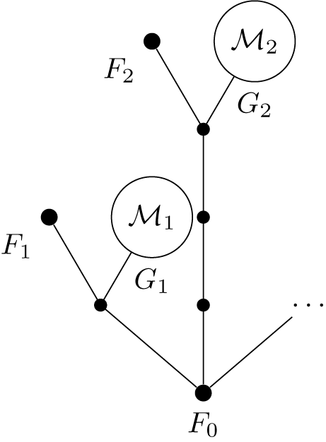


 Open access