1. Introduction

In a seminal paper, Furbish and Andrews (1984) showed that the hypsometry (area–altitude relationship) of a glacier plays a critical role in the response of the terminus to changes in equilibrium-line altitude (ELA). Furbish and Andrews (1984) considered five idealized but representative shapes of valley glaciers, originally proposed by Osmaston (1975), and analyzed the response of their termini to vertical shifts in ELA assuming a piecewise linear mass-balance profile. The five idealized classes comprise glaciers with a uniform hypsometry, i.e. area is constant with elevation (shape A); glaciers where the bulk of area lies above the ELA (B); glaciers where the bulk of area lies below the ELA (C); glaciers where the bulk of area lies at the ELA (D); and glaciers with bimodal hypsometric curves, where the ELA lies approximately between the two bulges (E). Furbish and Andrews (1984) found that the termini of glaciers with shape B are initially most sensitive, i.e. their termini will experience the largest altitudinal change for a given shift in ELA. The termini of glaciers in shape classes D, A, E and C follow in order of sensitivity. The sensitivities are, however, nonlinear functions of hypsometry, and the final altitude that the terminus of a glacier reaches to accommodate a given change in ELA depends on the shift in ELA and the initial terminus altitude. The results convincingly demonstrated that the termini of glaciers with different hypsometry behave differently under similar climate forcing, highlighting the fundamental importance of geometry as a control on the behavior of glaciers (e.g. Reference Jiskoot, Curran, Tessler and ShentonJiskoot and others, 2009), an aspect that deserves consideration in assessments of glacier variations in the context of current climate change. In this paper, we look at the problem from a different angle, focusing on the role of hypsometry in the sensitivity of the mass balance to vertical shifts of the ELA: dḂ/ dELA. We begin by explicitly formulating dḂ/ dELA in terms of hypsometric and mass-balance functions, and derive a generic expression valid for any glacier and mass-balance curve. Then, relying upon a new glacier inventory and publicly available elevation data, we apply the concept to estimate the sensitivity of the simulated mass balance of 139 glaciers in the Southern Patagonia Icefield to vertical shifts in ELA. Our purpose is to assess whether we can confidently use the relatively accessible information on hypsometry and ELA as a first-order estimator of the climate sensitivity of unmeasured glaciers. Such an approach could provide means of qualitatively assessing the sensitivity of glaciers located in regions where contemporaneous series of climate and mass-balance data are scarce, and for which the climate sensitivity cannot be calculated in the standard way (e.g. Reference OerlemansOerlemans and others, 1998; Reference Braithwaite and ZhangBraithwaite and Zhang, 2000).

2. Concept, Data and Methods

2.1. Concept

We seek an expression for the sensitivity of the mass-balance rate to changes in ELA that is based on easily measured properties and that can be applied to a wide range of glaciers, irrespective of their balance state or boundary condition at the terminus. For simplicity, we restrict ourselves to the static case, i.e. for the current geometry of glaciers under small perturbations of ELA. We assume that mass balance is only a function of altitude, neglecting horizontal gradients and complex spatio-temporal variability due to avalanches and wind redistribution of snow (e.g. Reference Machguth, Eisen, Paul and HoelzleMachguth and others, 2006). We also consider that variations of frontal ablation with ELA in calving glaciers are negligible: dḊ/ dELA ≈ 0. We justify this assumption on the basis that calving flux is primarily controlled by frontal geometry and basal conditions (e.g. Reference Benn, Warren and MottramBenn and others, 2007), which we here consider fixed. We also assume that variations in melting, evaporation and sublimation at the calving face due to ELA migration are negligible in comparison with attendant changes on the much larger glacier surface.

We begin by expressing the mass-balance sensitivity in terms of the accumulation–area ratio (AAR, the ratio of accumulation area to total area), its derivative against altitude (dAAR/dELA, equivalent to the area fraction vs elevation curve), and quantities derivable from a mass-balance model or observations. The balance equation for a glacier can be expressed as

(1)

where Ḃ is the net mass-balance rate, Ḃ _acc is the balance rate of the accumulation area, A _c is the accumulation area, Ḃ _abl is the balance rate of the ablation area and A _a is ablation area. Dividing both sides by the total area, and recalling the definition of AAR,

(2)

Eqn (1) can be rewritten as

(3)

We then take the derivative against ELA and rearrange to obtain

(4)

This equation explicitly expresses the change of mass-balance rate against a change in ELA in terms of hypsometric parameters and mass-balance quantities that can be derived from observed or modeled data. For simplicity, in the remainder of this paper we refer to the terms on the right-hand side as α, β and γ. The units of these terms are mass fluxes per unit ELA change (e.g. kilograms per square meter per year per meter of ELA change, kg m^-2 a^-1 m^-1, or equivalently, meters water equivalent per year per meter of ELA change, m w.e. a^-1 m^-1). Here we use the latter, presented as values per unit area of glacier, i.e. specific mass balance (Reference CogleyCogley and others, 2011), and, for convenience, as per 100 m ELA change.

2.2. Mass-balance model

The mass-balance quantities in Eqn (4) were derived for each glacier using a model that gives the mass balance as a function of elevation. We used a degree-day scheme with stochastically simulated precipitation, based on values of average annual temperature, lapse rate and estimated accumulation reported for an automatic weather station operating near the snout of Glaciar Perito Moreno (Reference Rott, Stuefer, Siegel, Skvarca and EckstallerRott and others, 1998; Reference Stuefer, Rott and SkvarcaStuefer and others, 2007). Daily values of air temperature and precipitation were calculated at 10 m elevation intervals. The evolution of daily temperatures during the year was modeled as a sine wave of mean 5.6°C, amplitude 7.2°C (at 180 m a.s.l.) and yearly frequency, plus normally distributed random noise with zero mean and 0.2°C standard deviation. A lapse rate of –0.008°C m^-1 was used. Daily precipitation was stochastically simulated using a first-order Markov chain (e.g. Reference WooWoo, 1992), where the probability of precipitation is 0.85 if there was precipitation on the previous day, and 0.55 otherwise. The amount of precipitation was simulated using a gamma distribution with shape and scale parameters equal to 1, multiplied by a constant of 0.05 m. This particular distribution was chosen because it allows us to impart a realistically large variability in daily precipitation values (e.g. a long-tailed distribution). The distribution parameters were tuned in order to obtain an average accumulation close to 5.5 m w.e. a^-1, as derived by Rott and others (1998). Our modeled values are also consistent with recent observations on the upper accumulation area of Glaciar Pío XI, where accumulation values of 3.4–7.1 m w.e. a^-1 have been reported (Reference Schwikowski, Schla¨ppi, Santiban˜ez, Rivera and CasassaSchwikowski and others, 2012). Precipitation was counted as accumulation if the temperature was lower than +1°C. Ablation was parameterized using a degree-day factor of 0.0065 m w.e. °C^-1 d^-1 for ice, and 0.0035 m w.e. °C^–1 d^-1 for snow (e.g. Reference HockHock, 2003). Water produced by melting or falling as rain was assumed to drain away from the glacier. Annual precipitation was assumed to increase with elevation with a factor of 0.0015 m w.e. m^-1 (based on Reference KuhnKuhn, 1981). The daily mass balance was calculated by subtracting the ablation from the accumulation. The balance profile used in the calculations was taken as the average of the outcomes of 100 model years (Fig. 1a).

Fig. 1.

Profiles of mass balance discussed in this paper. (a) The stochastic model used here, computed using data from Glaciar Perito Moreno. The central (bold) curve is the average of 100 modeled years, flanked by curves of one standard deviation. (b) A piecewise linear model of the same type as those considered by Furbish and Andrews (1984).

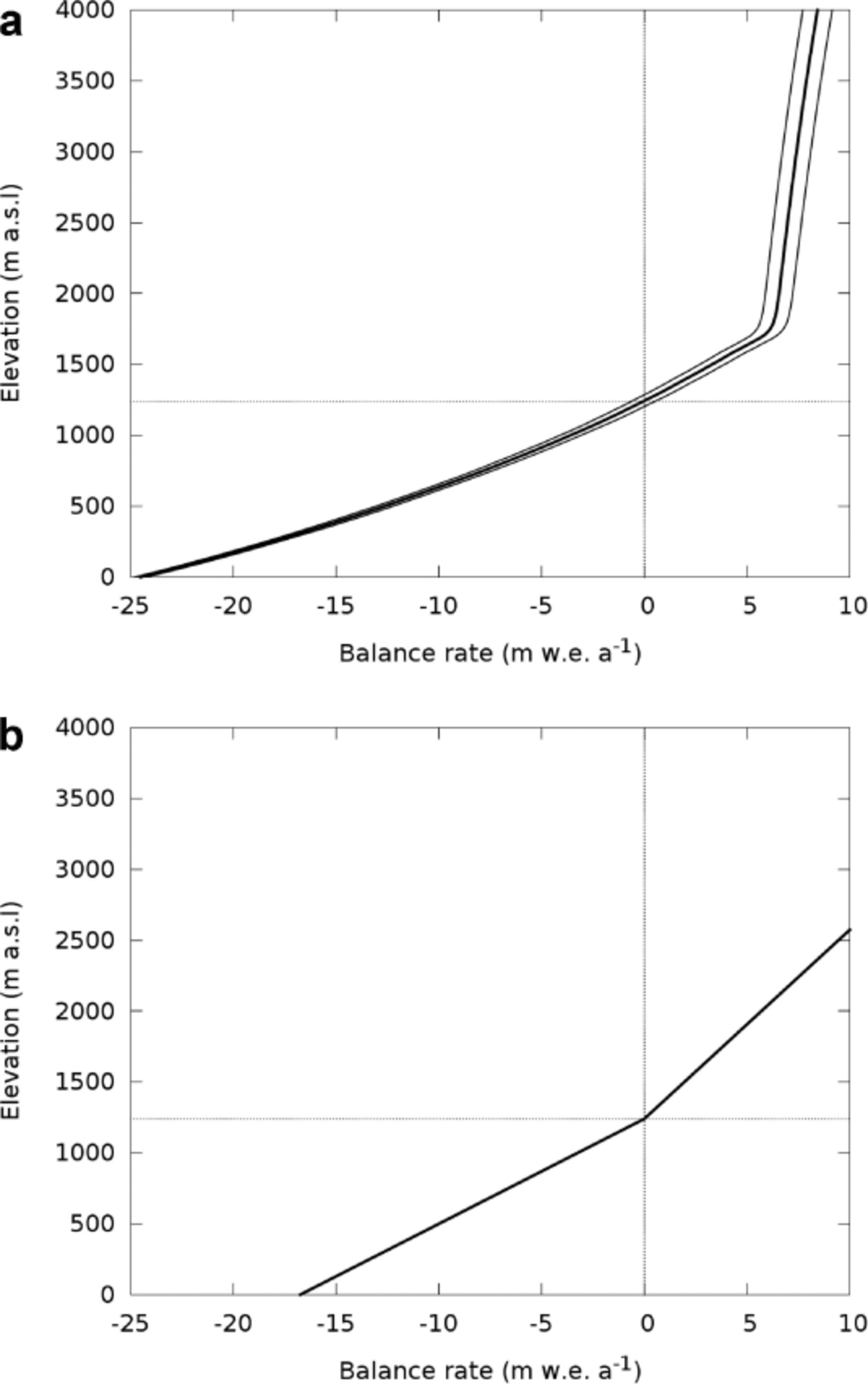
The resulting balance profile was applied to all glaciers, shifting the curve vertically to adjust for each individual ELA. The values of balance quantities in Eqn (4) were calculated by moving the balance profile vertically along the vertical span of each glacier, thus simulating equilibrium-line migration from the tongue to the top. It is important to stress that the purpose of this model is not to perfectly mimic the real balance field of every glacier, but to provide a plausible and realistic mass-balance curve for the region, that is suitable for testing the effects of hypsometry on balance sensitivity. Strictly speaking, the mass-balance parameters in Eqn (4) are dependent on details of the mass-balance model and aspects of the regional climate (e.g. the west–east gradients) that are outside the scope of this study and our simple model. For this reason, error bounds in the mass-balance quantities were not calculated. In order to support the discussion, summaries of the results are also presented for the case of a piecewise linear mass-balance model of the type considered by Furbish and Andrews (1984), with constants dḂ/ dz = 0.0135 m w.e. m^-1 for z < ELA (based on Reference RiveraRivera, 2004) and dḂ/ dz = 0.0075 m w.e. m^-1 for z > ELA (Fig. 1b).

2.3. Glacier inventory of the Southern Patagonia Icefield

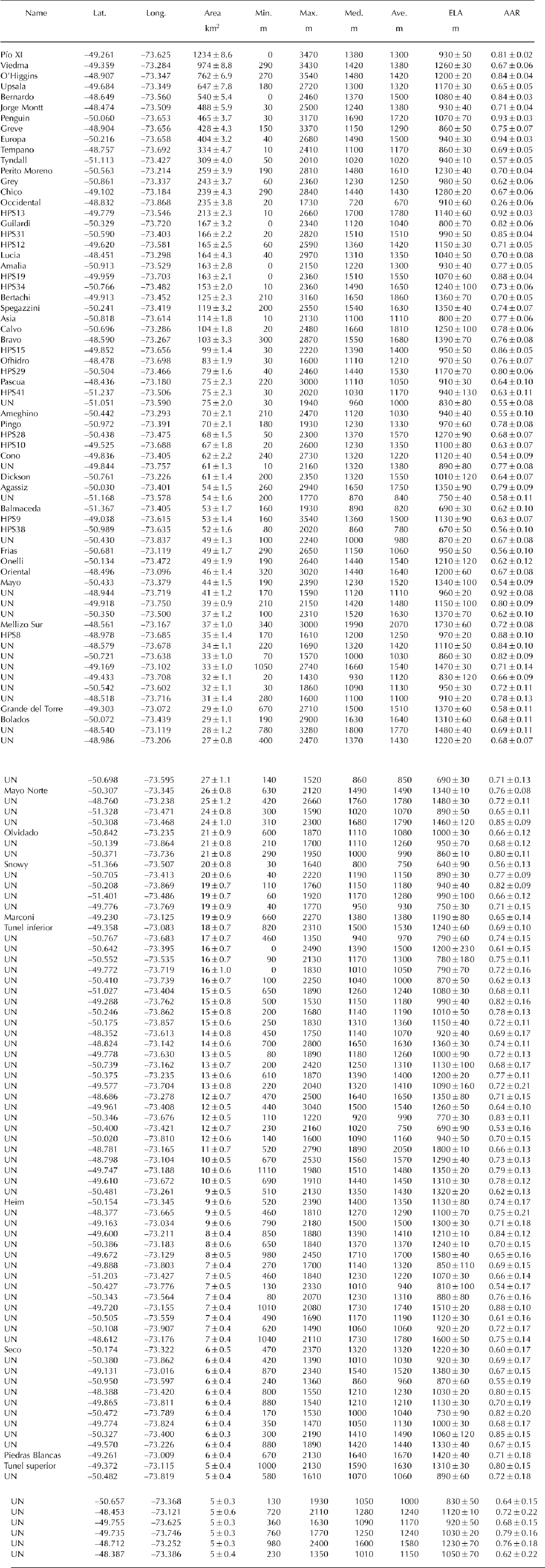
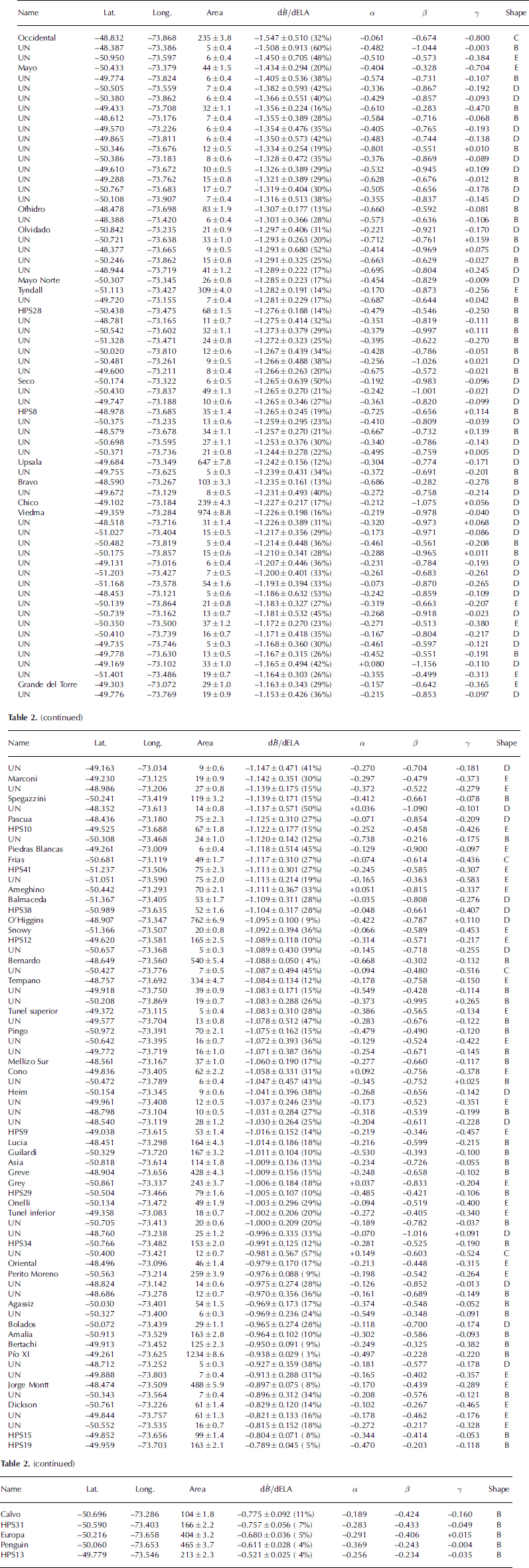
In this paper we rely on a new inventory of the Southern Patagonia Icefield, using the outlines as masks for extracting the hypsometry of individual glaciers from the elevation model (Fig. 2; Table 1). Glaciers were manually outlined after visual interpretation of exceptionally cloud-free Land-sat 5 Thematic Mapper (TM) images acquired on 12 March 2001 (Skvarca and De Reference Skvarca and De AngelisAngelis, 2003). The boundaries over low-relief plateaus were defined with minimal ambiguity with the aid of a shaded relief model (16× vertical exaggeration) and artificially computed ‘water drainage flowlines’, both derived from Shuttle Radar Topography Mission (SRTM) data (Reference FarrFarr and others, 2007). The newly compiled outlines generally coincide with those of Aniya and others (1996), derived using Landsat 5 TM images acquired in January 1986. The largest discrepancies are found for Pío XI, Viedma and Upsala glaciers, which Aniya and others (1996) reported to be 1265, 945 (maximum) and 902 km² in area, but are here found to be 1234, 974 and 835 km², respectively (Table 1). These discrepancies are explained by the slightly different choice of ice divide at some locations and by glacier retreat between January 1986 and March 2001 (Reference Davies and GlasserDavies and Glasser, 2012). Although the reported differences do not invalidate the work of Aniya and others (1996), we note that the inventory presented here was compiled using completely cloud-free images and the explicit aid of SRTM topography, both of which were unavailable to Aniya and others (1996). The new inventory contains 139 glaciers larger than 5 km², covering a total area of 12 363 km², and is now part of the Randolph Glacier Inventory, version 2 (RGI; Reference ArendtArendt and others, 2012).

Table 1.

Glacier inventory of the Southern Patagonia Icefield. Glaciers are reported in descending order of area. Unnamed glaciers referred to as ‘UN’

Errors in the digitization process were quantified by assuming that the uncertainty in the placement of the margin is half a pixel of the reference image (15 m). In this way, we treated the glacier margin as a 30 m wide buffer whose area, obtained by multiplying the perimeter of the glacier by the buffer width, gives a reasonable estimate of the total area uncertainty of the glacier. Glaciers smaller than 5 km² were not considered to keep the area uncertainty under 10%. The same criterion applies to nunataks smaller than 10 pixels (~9000 m²) since their inclusion would increase the total uncertainty by an amount larger than their actual areas.

2.4. Glacier hypsometry

We use SRTM data as elevation reference due to their high quality and consistency as a topographic ‘snapshot’, acquired during 2 weeks in February 2000 (Reference FarrFarr and others, 2007), 13 months before the satellite images used to compile the inventory. Voids in the original data were filled by using the elevation cells to generate a new elevation grid using bilinear interpolation. The voids were relatively small and mostly located on steep slopes, so the errors introduced by this procedure were negligible for our purposes. The elevation data were then extracted for every glacier using the boundaries in the inventory as masks. The hypsometric curves were generated by creating histograms of the elevation data with a 10 m bin size. The AAR vs elevation curve was then obtained by integrating the hypsometric curves and normalizing them to the range 0–1.

Fig. 2.

Glacier inventory of the Southern Patagonia Icefield compiled for this study. Full lines show the elevation contours of the current average ELA. Dashed lines show contours spanning the uncertainty range. The background image was obtained by averaging seven cloud-free Moderate Resolution Imaging Spectroradiometer (MODIS) images acquired in the late summers of 2002 and 2004.

2.5. Equilibrium-line altitudes

We here approximate equilibrium lines as snowlines at the end of the ablation season, following the usual convention for temperate glaciers. The snowlines were automatically detected on an average of seven cloud-free images acquired by the Moderate Resolution Imaging Spectroradiometer (MODIS) in the late summers of 2002 and 2004 (Fig. 1). We use an average of images instead of single images because the averaging process smooths out random noise and other irrelevant fluctuations, highlighting the long-term features of interest. We use MODIS data because the high revisit frequency increases the likelihood of acquiring cloud-free images. The relatively coarse pixel size (250 m) is of minor importance here because of the large size of the icefield and the broad scope of the study. The images were acquired on 5, 16 and 17 February 2002; 5, 6 and 7 February 2004; and 10 March 2004. Snow cover was then at or very close to the seasonal minimum. Before averaging, the raw images were converted to top-of-the-atmosphere radiance, then topographically corrected using the void-filled SRTM data and finally converted to surface reflectance using standard algorithms (Reference SchowengerdtSchowengerdt, 2006).

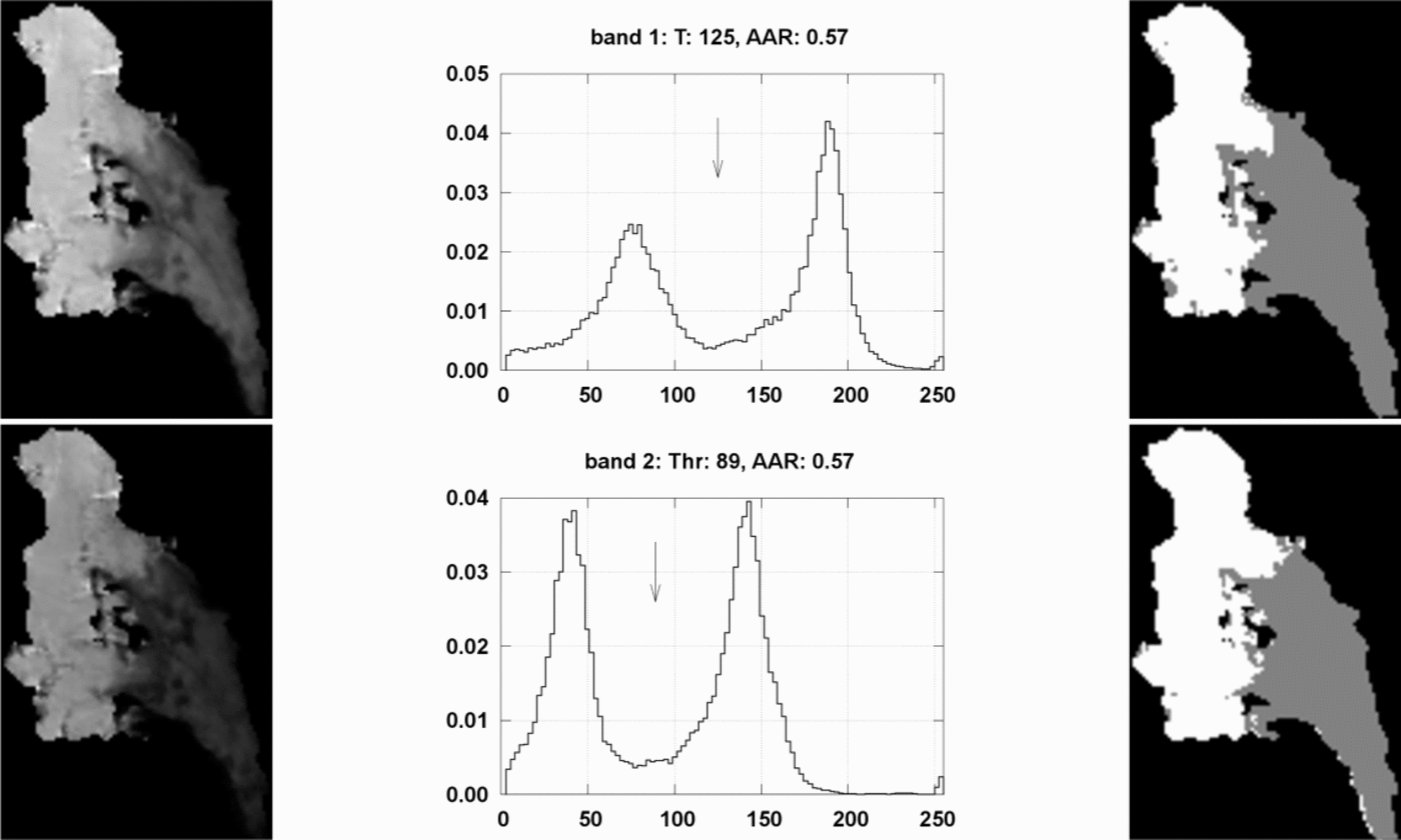
Glaciers were automatically segmented into accumulation and ablation areas using Otsu’s optimal thresholding method (Reference OtsuOtsu, 1979). The procedure is optimal in the sense that it finds the threshold that maximizes a separability function between two classes (Reference Gonzalez and WoodsGonzalez and Woods, 2008). The suitability of the technique for our purposes is justified on the basis of the good spectral separability between glacier facies that can be safely assumed to represent accumulation and ablation areas (Reference Williams, Hall and BensonWilliams and others, 1991), a criterion that has been successfully applied to the Southern Patagonia Icefield (Reference Aniya, Sato, Naruse, Skvarca and CasassaAniya and others, 1996; De Reference De Angelis, Rau and SkvarcaAngelis and others, 2007). Otsu’s optimal thresholding performed extremely well in most cases, and yielded the least ambiguous results in all experiments run in the context of this study, in which several alternative methods were tested, including maximum likelihood classification and linear spectral unmixing (Reference Klein and IsacksKlein and Isacks, 1999). For each glacier, ablation and accumulation areas were automatically separated by applying Otsu’s thresholding to the red and near-infrared bands (band 1, 0.62–0.67 mm; and band 2, 0.841–0.876 mm) and the first two principal components derived from bands 1–7 (visible to mid-infrared; Fig. 3). AAR was then calculated from each of these datasets and a final value obtained by averaging.

Fig. 3.

Example of automatic segmentation of Glaciar Tyndall into ablation and accumulation areas using Otsu’s optimal thresholding. The left column shows the base data: MODIS bands 1 (red) and 2 (near-infrared). The center column shows the histograms, where the abscissas represent image raw digital numbers and the ordinates data frequency. The arrows indicate the threshold value. The right column shows the segmented images with accumulation (white) and ablation areas (dark gray), from which AAR was calculated.

A representative, or effective, ELA was chosen as the elevation corresponding to the present AAR, as derived from the AAR vs altitude curve. This criterion relies on the one-to-one correspondence between AAR and elevation in the hypsometric function of each glacier, and has the advantage of being objective, reproducible and physically more meaningful than, for example, averaging the altitude values along the snowline. In a few cases, however, a mismatch occurs between the visually inferred snowline and the computed snowline plotted as a contour when the real snowline spans an altitude range on a very wide glacier (Fig. 1). The extreme cases are Glaciar Tyndall, in which the snowline altitude differs by >100 m between its two accumulation basins, and Glaciar O’Higgins, in which the southern portion of the snowline is forced downwards as a result of the prominent wind deflection of snow around Volcán Lautaro (De Reference De Angelis, Rau and SkvarcaAngelis and others, 2007). In most cases, however, the mismatch is negligible and the approximation works well. Uncertainties in AAR were conservatively taken as the standard deviation of the four AAR values used to extract the average, but are probably larger in glaciers where the transition zone between firn and ice is very wide (de Ruyter de Reference De Ruyter de Wildt, Oerlemans and BjörnssonWildt and others, 2002).

3. Results

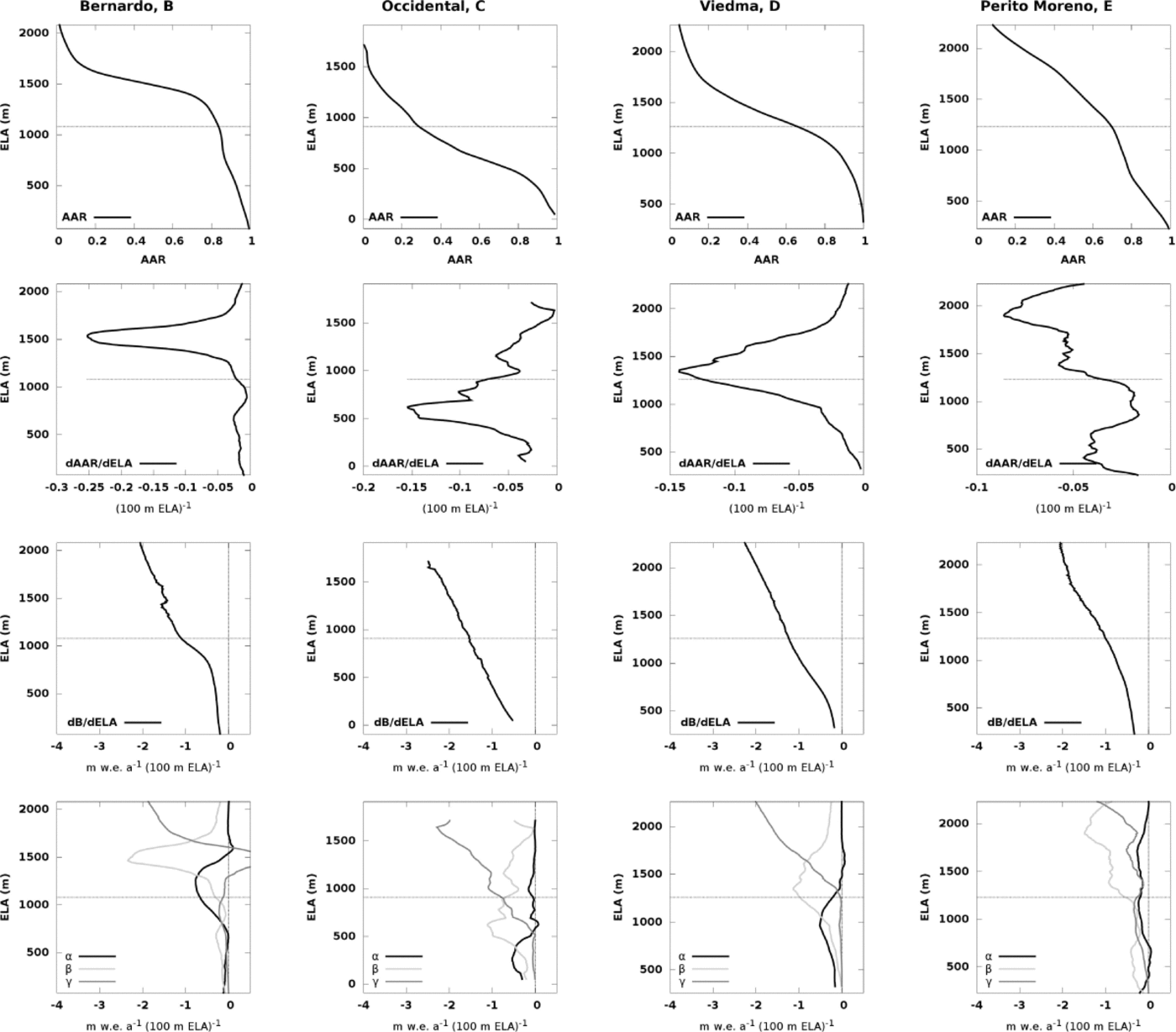
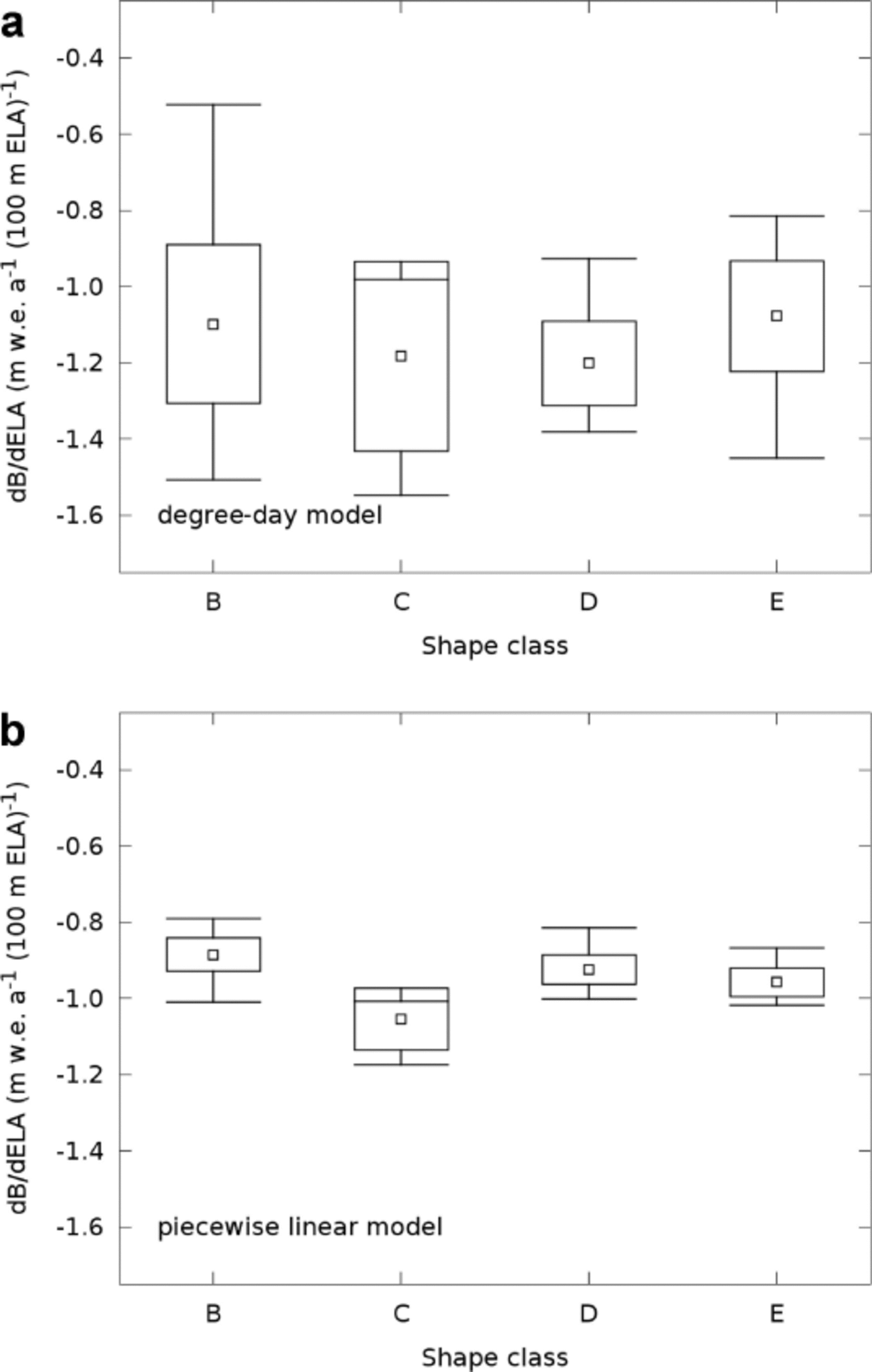
The terms in Eqn (4) were calculated and plotted as functions of ELA for the entire altitude range, as if the ELA were to migrate from the tongue to the top (Fig. 4). This approach is convenient for visualizing the role of hypsometry in the mass-balance sensitivity and the relative importance of the terms across the altitude range, but we stress that the physically meaningful values are only those near the current ELA. Figure 4 shows the hypsometric curves and sensitivity functions calculated with the degree-day model for four glaciers, closely corresponding to the ideal shape classes B–E of Furbish and Andrews (1984). Values of AAR, dḂ/ dELA, α, β and γ in the vicinity of the current ELA (±25 m), as well as the shape class for all 139 glaciers, are shown in Table 2. The uncertainty in dḂ/ dELA was estimated by propagating the errors in AAR and dAAR/dELA: ΔdḂ= dELA = (ΔAAR/AAR)α + 2ΔAARβ + (ΔAAR/AAR)γ. The uncertainties tend to be larger for smaller glaciers because the area of the perimeter buffer tends to be large in comparison with the absolute area, and because the image segmentation analysis is based on a smaller number of pixels. Note that for the smallest glaciers (<10 km²) the values may be unreliable. Summary statistics of dḂ/ dELA, calculated for each class using both the degree-day and piecewise linear mass-balance models, are shown in Figure 5 and Table 3.

Table 2.

Mass-balance sensitivities for glaciers in the inventory, calculated using the degree-day model. Glaciers are reported in descending order of sensitivity, calculated using a degree-day mass-balance model. The units of the sensitivity terms are m w.e. a^-1 per 100 m ELA change. Values in parentheses are errors in dḂ/ dELA given as percentages. Unnamed glaciers referred to as ‘UN’

Table 3.

Summary statistics of dḂ/ dELA for all shapes using a degree-day and a piecewise linear mass-balance model

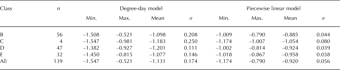
The average mass-balance sensitivity of the 139 glaciers is –1.131 ± 0.174 m w.e. a^-1 per 100 m ELA change when using the degree-day model, and –0.920 ± 0.056 m w.e. a^-1 per 100 m ELA change in the case of the piecewise linear model. As noted above, these values are approximations and should be used with care because the exact value of the sensitivity depends on details of the mass-balance model considered. Note, however, that the degree-day mass-balance model was built upon realistic and plausible choices, based on and consistent with observed data (Reference Rott, Stuefer, Siegel, Skvarca and EckstallerRott and others, 1998; Reference Stuefer, Rott and SkvarcaStuefer and others, 2007; Reference Schwikowski, Schla¨ppi, Santiban˜ez, Rivera and CasassaSchwikowski and others, 2012). We may therefore expect that the average value given by this model lies closer to the real regional value than the average given by the piecewise linear model. Calculations using both mass-balance models (Tables 2 and 3; Figs 4–6) show that glaciers where the bulk of area is located above the ELA (B) are the least sensitive, whereas those where the peak of area is below the ELA (C) are the most sensitive. Bimodal or multimodal glaciers where the ELA is between hypsometric peaks (E), and unimodal glaciers with bulges at roughly the ELA (D), have intermediate sensitivities that fall between those of classes B and C. Glaciers in shape class E tend to be less sensitive than those in shape class D under a nonlinear mass-balance field, but these two classes have approximately the same sensitivity when a piecewise linear mass-balance model is considered.

Fig. 4.

Hypsometric and sensitivity curves for (left to right) Bernardo, Occidental, Viedma and Perito Moreno glaciers, representing shape classes B–E as functions of ELA: row 1: AAR; row 2: dAAR/dELA; row 3: balance sensitivity dḂ/ dELA; row 4: α, β and γ. The horizontal dotted lines denote the current ELA. Vertical lines denote the zeroes on the x –axis for the different plots.

Fig. 5.

Summary of mass-balance rate sensitivity for the shape classes considered here. The central points represent the average sensitivity of the classes, the boxes enclose the range of one standard deviation above and below the mean, and the bars depict the range between minimum and maximum sensitivity. Note that there are only four glaciers in shape class C.

Fig. 6.

Mass-balance variation as a function of ELA shift from its current value for the four representative glaciers. Curves calculated using (a) the degree-day model and (b) the piecewise linear model.

For all shape classes, the mass-balance sensitivity to ELA is exacerbated by the nonlinearity of the model (Fig. 6). A linear mass-balance model, for example, with constant dḂ/ dz = 0.0132 m w.e. m^-1 (based on Reference RiveraRivera, 2004), yields a constant sensitivity across the altitude range, i.e. a vertical line (Fig. 7a). The piecewise linear model gives fairly similar results except for a smooth change in sensitivity arising from the different slopes of the two linear sections of the curve (Fig. 7b). On the other hand, the nonlinear degree-day model makes the sensitivity variation with ELA also nonlinear. In this case, independently of the individual hypso-metric characteristics, the mass-balance sensitivity increases, i.e. dḂ/ dELA becomes more negative, as the ELA rises (Fig. 7c). A nonlinear model tends to exacerbate the differences between the classes and the spread of the values within each of them (Fig. 5; Table 3).

Fig. 7.

Hypsometric components of mass-balance sensitivity for Glaciar Pío XI, in a linear (a), piecewise linear (b) and a nonlinear degree-day (c) mass-balance model.

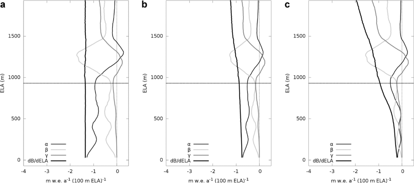
The relative importance of the terms α, β and γ and their variation with ELA remain, nevertheless, essentially the same, albeit modulated by the dḂ/ dELA curve in the piecewise and nonlinear case. The clearest and most consistent pattern of variation with ELA is that of β, which follows the curve of area fraction, dAAR/dELA, and is often the numerically dominant term where the ELA coincides with bulges of area (e.g. Glaciar Viedma in Fig. 4). The first term, α, becomes more important towards the lower reaches, but in the examples calculated with the nonlinear degree-day model this becomes less clear because the sensitivity functions approach zero towards the snout. The last term, γ, follows the opposite trend, becoming numerically important when the ELA lies close to the upper reaches of the glacier, when AAR is low.

4. Discussion

Glaciers in shape class B are characterized by unimodal area distributions, with the bulk of area located above or well above the present ELA and thus having high AAR values. This class is exemplified by Glaciar Bernardo (Fig. 4) and includes large glaciers such as Pío XI, Europa and Penguin. These glaciers are the most numerous in our study and have the lowest mass-balance sensitivities. Most of these glaciers are located on the western side of the icefield and all have calving termini. In general, α and β tend to dominate the total sensitivity: α does so when AAR is large, whereas β does so when the hypsometric mode is close to the ELA. On the other hand, γ is naturally unimportant since it depends on the complement of the AAR, which is consistently low in these glaciers (Table 2). Furbish and Andrews (1984) found that the termini of these glaciers are the most sensitive, those that will experience the largest changes in elevation in reaching equilibrium after a change of ELA. There is no contradiction here with our findings: glaciers in shape class B have long and narrow tongues usually lying at lower altitudes than the termini of glaciers in other shape classes. In these conditions, even slight changes in the net mass balance will translate into relatively large altitudinal shifts of the terminus, whereas little change will be experienced at higher altitudes. Note, however, that all glaciers with shape B in our study have calving termini. The terminus altitude is thus bound to the water level, except when large changes in mass balance promote retreat to higher elevation beyond the water body. For small changes in ELA, mass-balance changes affecting the tongue are accommodated by horizontal shifts of the calving front position (Reference MercerMercer, 1961).

Glaciers in shape class C, exemplified by Glaciar Occidental, have roughly unimodal area distributions with the bulk of area below the present ELA, thus showing low AAR values. These glaciers have opposite properties to those in shape class B, showing the highest mass-balance sensitivities, primarily dominated by γ and secondarily by β. Furbish and Andrews (1984) found that the termini of these glaciers are less sensitive to changes in ELA than those in all other classes. The geometric properties of their ideal class are opposed to those in shape class B, with wide ablation areas lying at higher elevation and relatively closer to the ELA. In these conditions, the altitudinal adjustment of the tongue to a given imbalance will be smaller than a similar change for other classes. In our study area, only a handful of glaciers have hypsometric curves of this type. All of them except Glaciar Occidental are smaller than 50 km² and show signs of marked retreat (e.g. Glaciar Frias). Nonetheless, in contrast with the ideal shapes of Furbish and Andrews (1984), these glaciers do not have wide ablation areas close to their present ELA. The mass-balance fields that would be necessary to maintain such glaciers in steady state – high accumulation on small accumulation areas balanced by low ablation on large ablation areas – are unlikely to prevail in the region and are incompatible with the balance requirements of neighboring glaciers. It is therefore likely that these glaciers have evolved under different climate conditions, presumably with lower ELA than at present, and are currently changing their geometry to adapt to new mass-balance fields. The exception seems to be Glaciar Occidental, which stands out as an anomaly. It tops the sensitivity list (Table 2) with the most negative value of dḂ/ dELA, it has a very low AAR (0.26) and most of its area is well below the ELA, although it does not show signs of marked retreat or instability in its elongated tongue (Fig. 1). It seems unlikely that such a relatively healthy glacier might have developed this hypsometry under the constraints of the prevailing balance field. This suggests that, from a dynamical point of view, it is probably more correct to consider Glaciar Occidental as part of a much larger and complex glacier, encompassing Greve and Tempano glaciers. Such a glacier would cover an area of 998 ± 8 km², with an AAR of 0.65 ± 0.08, a multimodal area distribution and a dḂ/ dELA of around –1.10 ± 0.23 m w.e. a^-1 per 100 m ELA (using the degree-day model), characteristics that would put it into shape class E.

Glaciers with unimodal area distributions where the bulge of area is located at or very close to the ELA have sensitivities that are intermediate between classes C and B, being about as sensitive as class E when considering a piecewise linear mass-balance model but more sensitive than this in the case of the nonlinear degree-day model. These glaciers correspond to the idealized shape D, exemplified by Glaciar Viedma, and including Upsala, O’Higgins and Chico, all located on the eastern side of the icefield. A consistent feature of these glaciers is that the dominant component of the sensitivity is the term β, related to the area fraction, dAAR/dELA, whereas the other two terms are of secondary importance. This is interesting because it reveals the impact of the character of the climate setting on the mass-balance sensitivity of this type of glacier. Recalling from Eqn (4) that β = (dAAR/dELA)(Ḃ _acc – Ḃ _abl), we see that the term multiplying the area fraction is subject to change according to the climate setting. In a relatively continental climate, both Ḃ _acc and Ḃ _abl tend to be lower than in a maritime environment, so their difference will be smaller, resulting in a reduced mass-balance sensitivity for the entire glacier. The same can be applied to the case of a given glacier exposed to natural interannual variability, in which the glacier will show higher sensitivity during years with a more maritime climate. This reasoning possibly explains why most glaciers in this shape class are located on the eastern side of the icefield, which is under a more continental climate than the western side. Glaciers, as adaptive systems, have attained geometries with low average sensitivities for the prevailing conditions which are thus conducive to long-term stability.

Glaciers in shape class E have bimodal and sometimes multimodal area distributions, with the ELA roughly located between two hypsometric modes. These glaciers, exemplified by Glaciar Perito Moreno, tend to have, on average, higher sensitivities than glaciers in shape class B, but lower sensitivities than those of class C. When considering nonlinear mass-balance models, these glaciers also tend to be less sensitive than those in class D. Other glaciers in this class are Mayo, Ameghino and Jorge Montt. In these glaciers, the relationship between the terms in Eqn (4) is comparable with that of glaciers in shape class B, with no clear pattern and often being dependent on the exact location of bulges in area fraction that make β dominant. The apparently contradictory inclusion of Perito Moreno, a remarkably stable glacier (Reference Skvarca, Naruse and De AngelisSkvarca and others, 2004), together with Ameghino and Jorge Montt, glaciers that have retreated or are currently retreating catastrophically (Reference WarrenWarren, 1994; Reference Rivera, Corripio, Bravo and CisternasRivera and others, 2012), in this group of relatively low-sensitivity glaciers merits explanation. The collapses of the tongues of Ameghino and Jorge Montt glaciers belong to the well-known class of calving retreat process which, although triggered by a climatically driven surface thinning, is sustained by positive feedback between mechanical extension, thinning and retreat (e.g. Reference Benn, Warren and MottramBenn and others, 2007). These phenomena are related to the theme of this paper only as the particular way in which certain glaciers react to particular boundary conditions, adapting their hypsometry to a changing climate, but have in principle no bearing on the glacier-wide mass-balance sensitivity to changes in ELA. Furbish and Andrews (1984) found the termini of these glaciers were less sensitive than those of shape class B, but more sensitive than the other classes.

We can summarize our results and observations by noting that glaciers where the bulk of area is located above the ELA (B) tend to be the least sensitive to variations in ELA, whereas glaciers in which the bulk of area is below the ELA (C) tend to be the most sensitive, independently of the exact choice of mass-balance model. Glaciers with bi- or multimodal area distributions where the ELA is between peaks (E), and unimodal glaciers with bulges at roughly the ELA (D), have mass-balance sensitivities that lie between classes B and C. The sensitivities of glaciers in classes D and E lie approximately in the same order of magnitude when a piecewise linear mass balance is considered, but glaciers in shape class E tend to be less sensitive than those of class D under a nonlinear mass-balance field. A nonlinear mass-balance field tends to exacerbate the differences between the classes, whereas a linear mass-balance model renders the sensitivities of all classes the same, and equal to the slope of the model. Accordingly, we suggest that a static, first-order estimation of the mass-balance rate sensitivity of a glacier can be obtained from its hypsometry by assessing the location of the peaks of area fraction (dAAR/dELA) relative to the ELA. The requirements are very simple, comprising only knowledge about hypsometry, average ELA and reasonable, although not necessarily too accurate, assumptions about the prevailing mass-balance field. We have shown that these data can be reliably acquired using a glacier inventory, and publicly available elevation data and satellite images, by applying relatively simple procedures. We suggest that the ideas expressed in this paper can be used to make reasonable first-order estimations of the mass-balance sensitivity of unmeasured glaciers. More accurate assessments can be derived by recalculating the sensitivities using a more adequate mass-balance model, possibly derived from measurements or from a more appropriate model. We remind the reader that we refer here to static sensitivity of the mass-balance rate against a reference mass balance, where we held the glacier area constant. We do not consider the dynamic case, where glaciers adapt their profiles to a changing mass-balance profile.

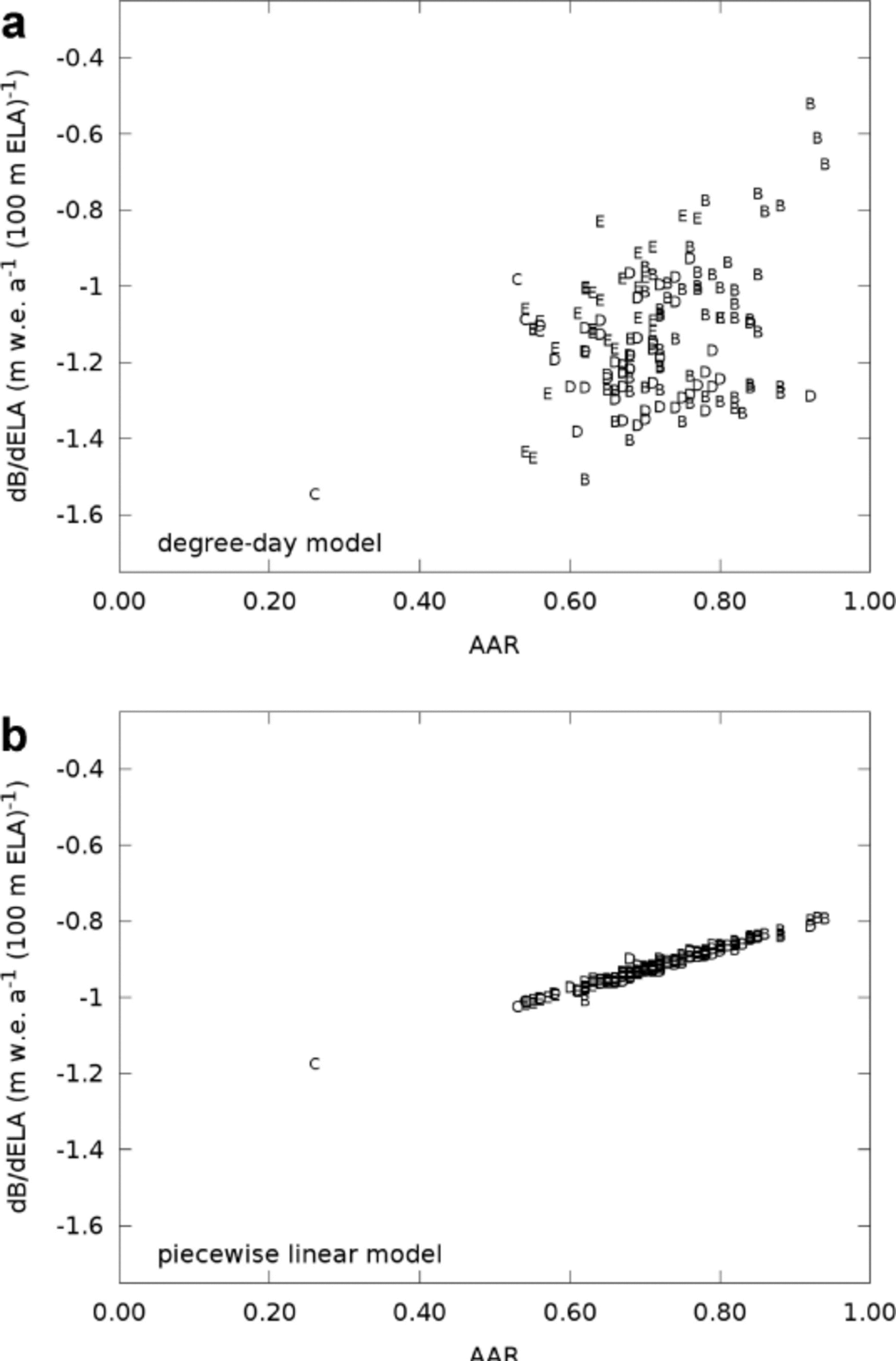
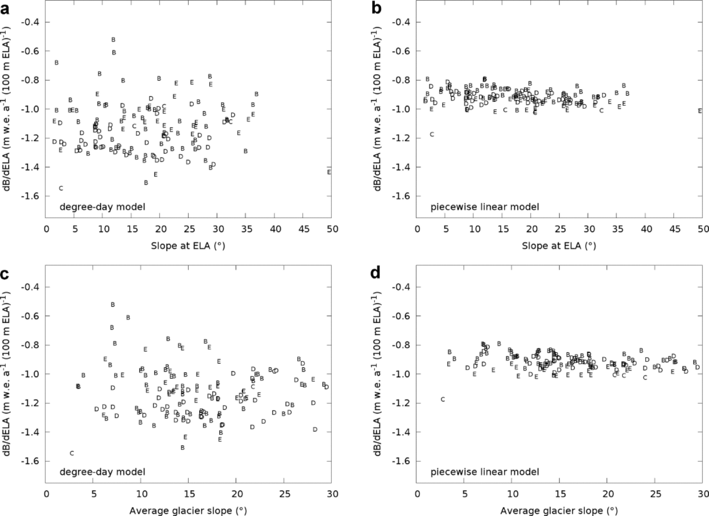
An interesting observation is that, when using a degree-day model, the mass-balance sensitivities of the shape classes and the respective sensitivities of the termini found by Furbish and Andrews (1984) are roughly in inverse order, i.e. glaciers with high (low) mass-balance sensitivity tend to have low (high) terminus sensitivity. The order of mass-balance sensitivities is also reflected in a positive correlation between AAR and sensitivity, such that glaciers with high AAR values tend to be less sensitive to variations in ELA (Fig. 8). Note how the presence of a nonlinear mass-balance field makes the relation less clear, blurring the correlation. Our dataset can also be used to probe the commonly held view that a glacier on which the area around the equilibrium line is steep should be less sensitive to variations in ELA than a glacier on which that sector has a shallow surface slope. Contrary to this view, our numerical experiments using the nonlinear degree-day model showed that the surface slope, either in the vicinity of the equilibrium line or averaged over the glacier, has little bearing on mass-balance sensitivity (Fig. 9). Values of sensitivity calculated using the piecewise linear model fall along an apparent line, but this relationship is also not significant, because the slope of that line would be close to zero. Note that a commonly cited explanation for the observed stability of Glaciar Perito Moreno is that the steep slope near the equilibrium line minimizes the effects of equilibrium-line variations (Reference Aniya and SkvarcaAniya and Skvarca, 1992; Reference Pasquini and DepetrisPasquini and Depetris, 2011). However, our analysis and data clearly indicate that in this case the sensitivity is a more complicated function of hypsometry and the local balance field.

Fig. 8.

Sensitivity vs AAR for the 50 largest glaciers. Symbols refer to hypsometric shape class.

Fig. 9.

Sensitivity vs glacier slope at ELA (a, b) and average slope (c, d) for the 50 largest glaciers, calculated using the degree-day model (a, c) and the piecewise linear model (b, d). Symbols refer to shape classes.

In this regard, it is also important to note the generally inverse relationship between the sensitivity to changes in ELA of the altitude of the terminus, as found by Furbish and Andrews (1984), and that of the mass balance, as found here. This apparent paradox occurs because of the different ways in which changes in ELA affect the terminus altitude and the mass balance for different glaciers, both of which are sensitive to the nonlinearity of the interaction between hypsometry and the mass-balance field. This observation is important for interpreting records of glacier length or ELA, and calls attention to potentially serious logical flaws in attempting to reconstruct climate histories from the inversion of such records (e.g. Reference Oerlemans, Dyurgerov and Van de WalOerlemans and others, 2007; Reference Leclercq, Oerlemans and CogleyLeclercq and others, 2011). As noted by Kuhn (1981) in an information-theoretic or signal-processing analogy, such attempts are essentially efforts to invert a broadband filtered signal to reconstruct the input from at least two sources (temperature and precipitation), which can be fallacious. A more logically sound approach for exploiting long glacier records for such reconstructions could instead be to recast the inversion problem as one in probabilistic inference, where the data are used to update the likelihood of a set of hypotheses (e.g. Reference JaynesJaynes, 2003).

5. Conclusions

Hypsometry is an important control on the sensitivity of mass balance to changes in ELA in the presence of a nonlinear mass-balance field. The most fundamental aspect of this relationship, that can be used as a first-order estimator of the mass-balance sensitivity for unmeasured glaciers, is the location of peaks in the hypsometric curve relative to the average ELA. Glaciers in which the bulk of area is located well above the ELA are those in which the mass balance changes the least for a given change in ELA. At the opposite extreme, glaciers where the bulk of area is located below the ELA are subject to the largest changes of mass balance for any given change in ELA. These are the most sensitive and vulnerable glaciers, so there are very few of them in our dataset. Between these extremes lie two distinct groups: glaciers with unimodal hypsometric curves where the peak is around the present ELA, and glaciers with bi- or multimodal area distributions, with the ELA located approximately between the bulges. Under the influence of a nonlinear mass-balance field the latter tend to be less sensitive than the former, but both are approximately equally sensitive when a piecewise linear mass-balance model is considered. In general, a nonlinear mass-balance field exacerbates the differences between the classes, whereas a linear mass-balance model renders the sensitivities of all classes the same and equal to the slope of the model. Assessments of mass-balance sensitivity of unmeasured glaciers can be derived in a relatively straightforward manner by applying the principles described in this paper. The only requirements are glacier inventories, publicly available elevation data and satellite images, and reasonable, but not necessarily too accurate, assumptions about the mass-balance field.