
Income and class biases in political representation have attracted the attention of many political scientists in recent years. More than any other scholarly work, Martin Gilens’ (Reference Gilens2012) study of unequal policy responsiveness in the United States has stimulated research and debate on this topic. Sorting survey respondents by relative income and estimating the probability of policy change based on some 1,800 survey items asking about support for specific reform proposals, Gilens finds that the preferences of high-income citizens predict policy change, but the preferences of low-income and even middle-income citizens have no influence on policy outcomes when they diverge significantly from the preferences of high-income citizens. These findings have sparked lively debates among scholars working on American politics. One debate focuses on the frequency and extent of divergence in preferences between income groups.Footnote 1 Simply put, do low- and middle-income citizens lose out to affluent citizens all the time or only occasionally? And, perhaps more importantly, do they lose out on issues that truly matter to them or (mostly) on issues that are not so salient? A second debate concerns the causal mechanisms behind the income biases in policy responsiveness identified by Gilens and other scholars (e.g., Bartels Reference Bartels2016, Ellis Reference Ellis2017, Hayes Reference Hayes2013, and Rigby and Wright Reference Rigby, Wright, Enns and Wlezien2011, Reference Rigby and Wright2013).
This chapter seeks to contribute to the debate about the reasons for unequal responsiveness by bringing data from European countries to bear and, in particular, by exploring whether policymaking under Left-leaning governments is less biased than policymaking under Right-leaning governments. Less directly, our empirical analysis also speaks to the debate about the meaning of unequal representation by exploring policy responsiveness and partisan conditioning of policy responsiveness across different policy domains.
It is tempting to suppose that the income biases identified by Gilens and others represent a uniquely American phenomenon. Indeed, many explanations for unequal responsiveness advanced by students of American politics imply that we should observe much more equal policy responsiveness in countries with lower income inequality, stronger unions, lower income inequality in voter turnout, and less costly, publicly subsidized election campaigns. However, recent studies replicating Gilens’ research design find that policy responsiveness is also biased in favor of affluent citizens in Germany (Elsässer, Hense, and Schäfer Reference Elsässer, Hense and Schäfer2021), the Netherlands (Schakel Reference Schakel2021), Norway (Mathisen Reference Mathisen2023), and Sweden (Persson Reference Persson2023). In what follows, we summarize the main findings of these studies and reanalyze the data on which they are based.Footnote 2 While the original studies largely focused on overall differences in political influence between low-income and high-income citizens, our reanalysis focuses on differences between middle-income and high-income citizens and the conditioning effects of government partisanship. By focusing on responsiveness to the preferences of high-income citizens relative to middle-income citizens, we respond to a common critique of the literature on unequal responsiveness, viz., that it shows that the affluent are better represented than the poor – a finding that is arguably unsurprising and entirely consistent with the median voter theorem (cf. Elkjær and Klitgaard Reference Elkjær and Klitgaard2021).
Gilens (Reference Gilens2012: Ch. 7) finds that responsiveness is equally skewed in favor of affluent citizens regardless of whether Democrats or Republicans control Congress and the White House, but most studies of unequal responsiveness in the United States support the intuitive hypothesis that the Democrats represent low- and middle-income citizens better than Republicans (Becher, Stegmueller, and Käppner Reference Becher, Stegmueller and Kaeppner2018; Ellis Reference Ellis2017; Lax, Phillips, and Zelizer Reference Lax, Phillips and Zelizer2019; Rhodes and Schaffner Reference Rhodes and Schaffner2017). In comparative politics, there is a large literature examining the effects of government party affiliation on social spending, welfare-state generosity, redistribution, and other policy outcomes on which citizens’ preferences are polarized by income.Footnote 3 Much of this literature follows Garrett (Reference Garrett1998) in positing that governing Left and Right parties alike seek to maximize their reelection chances by boosting macroeconomic performance and also cater to the policy preferences of their core constituencies, with core constituencies of Left parties identified as risk-exposed wage-earners with relatively low earnings and the core constituencies of Right parties identified as occupational strata characterized by lower exposure to labor market risks and higher earnings.
This stylized differentiation of Left and Right parties and their core constituencies would lead us to expect that Left-leaning governments are more responsive to the policy preferences of low- and middle-income citizens, and less responsive to the preferences of high-income citizens than Right-leaning governments. However, more recent literature (e.g., Manwaring and Holloway Reference Manwaring and Holloway2022; Mudge Reference Mudge2018) suggests that the mainstream Left – Social Democratic (and Labour) parties – have undergone a profound transformation since the 1980s, moving toward the center and adopting policy priorities associated with the notion of a “Third Way.” Key features of this trend have been a move away from redistributive tax and spending policies and a focus on social investment, a policy shift apparently designed to appeal to new middle strata and, in particular, “socio-cultural professionals” (Gingrich and Häusermann Reference Gingrich and Häusermann2015). Against this background, we first analyze whether Left-leaning governments mitigate income biases in policy responsiveness across all issues included in our datasets. We then focus on economic and social policies with direct distributive implications and, finally, explore temporal change in the effects of government partisanship on unequal responsiveness in this policy domain.
To anticipate, our results confirm that government policies in the four countries that we analyze are more responsive to the preferences of high-income citizens than to the preferences of middle- and low-income citizens. We find that unequal responsiveness is less pronounced under Left-leaning governments in Germany, the Netherlands, and Sweden, but there is still bias in favor of the high-income citizens even under Left-leaning governments, at least in Germany and the Netherlands. The Norwegian case is a puzzling exception in that Left-leaning governments seem to favor the affluent more than Right-leaning governments. However, this inversion of partisan conditioning disappears when we restrict our analysis to economic and welfare issues. More tentatively, we also find some support for the proposition that partisan conditioning of unequal responsiveness on distributive issues has indeed diminished over time.
In what follows, we proceed directly to empirics, leaving theoretical issues for later discussion. The first section presents the data we analyze and addresses methodological issues. The second section looks at patterns of unequal responsiveness across our four countries and presents the results of estimating different regression models with support for policy change at the 10th, 50th, and 90th income percentiles as predictors of policy adoption. In the third section, we introduce government partisanship as a variable that conditions policy responsiveness to the preferences of different income groups. In the fourth section, we restrict the analysis to economic and welfare issues and, in the fifth section, we explore changes in partisan conditioning over time. The final section summarizes our empirical findings and discusses their implications for the debate on mechanisms behind income bias in political representation.
Data and Methodology
For each of the four countries included in our analyses, authors of this paper created original datasets that matched public opinion with policy outcomes. In so doing, we followed the approach set out by Gilens (Reference Gilens2012). To begin with, we identified questions in preexisting public opinion surveys that asked respondents to indicate whether they supported specific proposals for policy change. The selection of survey items was restricted to items that asked about policy changes that could be implemented at the national level and were worded in such a way that it was possible to determine whether the proposed change was implemented subsequent to the survey. For Sweden and Norway, the original datasets included questions about constitutional changes, but we have removed these questions from the analyses presented here. Note also that some questions in the original datasets and the merged dataset are phrased in terms of support for status-quo policy and that responses to such questions have been inverted to capture support for changing policy in a particular direction.Footnote 4
The merged dataset contains nearly 2,000 observations (survey items), covering a wide range of issues, from raising the retirement age and cutting taxes to immigration reform, construction of nuclear power plants, and the introduction of same-sex marriage. As shown in Table 2.1, the items are unevenly distributed across countries and over time. In the pooled analyses presented later, we ensure that each country carries the same weight by weighting individual survey items by the inverse of the total number of items for each country. (The weights are adjusted when we analyze subsets of survey items.)
Table 2.1 Survey items by country
| Country | N | Years | Sources |
|---|---|---|---|
| Germany | 266 | 1998–2016 | Commercial |
| Netherlands | 291 | 1979–2012 | Mostly public |
| Norway | 557 | 1966–2014 | Mostly commercial |
| Sweden | 844 | 1960–2012 | Public |
The research projects on which we draw then harmonized the income of survey respondents in the manner proposed by Gilens (Reference Gilens2012: 61–62), using percentile midpoints to generate estimates of the share of respondents at the 10th, 50th, and 90th percentiles who support policy change (henceforth P10, P50, and P90). An obvious and important limitation, to which we shall return, is that we do not have any information about the salience of proposed policy changes for respondents.
The dependent variable in our regression models is a dummy variable that takes the value of one if the policy change in question was enacted within a given time period after the survey and otherwise the value of zero. Like Gilens, we estimate the probability of a policy change in the direction preferred by respondents at different positions in the income distribution and do not take into account how much policy changed. For example, we treat all increases or decreases in unemployment benefits as equivalent, irrespective of their magnitude (unless the magnitude was specified in the survey question).
Using information from legislative records, government budgets, and newspaper articles, we coded survey items as adopted or not adopted within two and four years of the survey in which they appeared. The main results presented here are based on two-year windows for adoption, with results based on four-year windows (Gilens’ default) presented in the online appendix (Tables 2.A2 and 2.A8–9). We prefer two-year windows because they provide a more precise measure of government partisanship, but the results for four-year windows turn out to be very similar.Footnote 5
Our preferred measure of government partisanship is the combined share of cabinet portfolios held by left-wing parties (Social Democratic and Green parties), as reported on an annual basis by Armingeon, Engler, Leemann, and Weisstanner (Reference Armingeon, Engler, Leemann and Weisstanner2023). For each survey item, we calculate the average share of cabinet portfolios held by left-wing parties in the year of the survey and in the two or four subsequent years. As reported in the online appendix (Table 2.A11), we obtain substantively equivalent results if we instead measure government partisanship with a dummy for the office of prime minister being held by a Social Democrat and restrict the analysis to survey items with two-year windows in which there was no change of prime minister.
Table 2.2 reports average values for our partisanship variable as well as support for policy change at P10, P50, and P90 and the frequency of policy change by country. For now, suffice it to note that, over the time period(s) covered by our analyses, Left parties have participated in government more frequently and more extensively in Norway and Sweden than in Germany and, especially, the Netherlands.
Table 2.2 Average values of independent and dependent variables by country
| Germany | Netherlands | Norway | Sweden | |
|---|---|---|---|---|
| Policy change (two years) | 0.57 (0.50) | 0.20 (0.40) | 0.21 (0.41) | 0.13 (0.34) |
| P10 support | 0.55 (0.22) | 0.48 (0.22) | 0.48 (0.23) | 0.55 (0.21) |
| P50 support | 0.56 (0.21) | 0.48 (0.22) | 0.47 (0.23) | 0.53 (0.22) |
| P90 support | 0.57 (0.19) | 0.48 (0.21) | 0.46 (0.23) | 0.48 (0.21) |
| P90–P10 support | 0.02 (0.15) | −0.01 (0.15) | −0.02 (0.12) | −0.07 (0.13) |
| P90–P50 support | 0.01 (0.10) | −0.00 (0.11) | −0.01 (0.09) | −0.05 (0.12) |
| P50–P10 support | 0.01 (0.08) | 0.00 (0.08) | −0.01 (0.07) | −0.02 (0.07) |
| Left cabinet share | 0.45 (0.36) | 0.26 (0.14) | 0.57 (0.32) | 0.59 (0.43) |
Note: Standard deviations in parentheses.
We explore how government partisanship affects responsiveness to lowincome, middle-income, and high-income citizens by interacting our measure of government party affiliation with measures of P10, P50, and P90 support for policy change. To avoid the complications associated with interpreting interaction effects estimated with logistic regression models (e.g., Gomila Reference Gomila2021), we present results based on estimating linear probability models, with heteroskedasticity-consistent standard errors, throughout the paper.Footnote 6
It is important to keep in mind that the public opinion data that form the basis for our analyses refer to policy changes that were discussed in a particular country at a particular point in time. The issues captured by our data and the overall balance across policy areas differ within countries over time as well as between countries. A further complication has to do with the sources of the survey data. As indicated in Table 2.1, the German dataset relies exclusively on commercial surveys, while the Swedish dataset relies exclusively on publicly funded surveys designed by academic researchers and the Dutch and Norwegian datasets combine both types of surveys. According to our data, policy change is much more common in Germany than in Sweden (see Table 2.2), but this may well be because the survey sources are different in the two countries, commercial surveys being more likely to ask about policy changes currently being discussed by policymakers. Based on these data, we cannot say with any certainty that status-quo bias is stronger in Sweden than in Germany. More generally, cross-national differences in policy responsiveness must be interpreted with caution. However, our primary interest pertains to patterns of unequal responsiveness within countries – how government partisanship conditions responsiveness to P10, P50, and P90 – and, for this purpose, cross-country differences in the questions asked in surveys would seem to be less relevant. Moreover, cross-national and temporal variation in survey items becomes less of a concern when we focus on economic and welfare policies. The issues pertaining to this policy domain are quite similar across our four cases and have not changed so much since the 1980s.
Unequal Policy Responsiveness
We begin our empirical analysis by looking at overall policy responsiveness to the preferences of P10, P50, and P90 in our four countries. In so doing, we replicate the results of the underlying country studies and establish the baseline for our subsequent analysis of how government partisanship conditions income biases in policy responsiveness. As indicated at the outset, we focus more explicitly on the political representation of middle-income citizens relative to high-income citizens than in our previous work.
Figure 2.1 shows the bivariate coefficients that we obtain when we regress policy adoption within a two-year window on our measures of support for policy changes at P10, P50, and P90 in separate models. For comparison, we include equivalent estimates based on Gilens’ data for the United States.Footnote 7 We also show the results that we obtain when we pool data for the four European countries. (Confidence intervals in this and all subsequent figures are displayed at the 95 percent level.)

Figure 2.1 Coefficients for support by income on the probability of policy change (bivariate linear probability models with two-year windows)
Note: See Table 2.A1 in the online appendix for full regression results.
While overall responsiveness to public opinion varies across countries, unequal responsiveness appears to be a common feature of liberal democracies. In Germany, the Netherlands, and Sweden, the likelihood of policy change increases significantly with P90 support for policy change, but this is not the case for P50 support, let alone P10 support. The coefficients for P50 and P10 support almost clear the 95 percent significance threshold for the Netherlands, but they are indistinguishable from zero for Germany and Sweden. Among the four European countries, Norway stands out as the only country where support for policy change at any point in the income distribution increases the likelihood of adopting policy changes, though the effect becomes stronger as we move up the income ladder. In this respect, Norway resembles the United States. As measured here, income biases in unequal responsiveness are more pronounced in Germany, the Netherlands, and Sweden than in the United States. Pooling our European data, the size of the coefficient for P50 preferences is about half the size of the coefficient for P90 preferences and the size of the coefficient for P10 preferences is about one quarter of the size of the coefficient for P90 preferences.
As commonly noted in the literature on this topic, the policy preferences of low-, middle-, and high-income citizens are correlated, and this renders the results presented in Figure 2.1 dubious. The effect of support for policy change among low- and middle-income citizens that we observe in the Norwegian and United States data may actually be the effect of support for policy change among high-income citizens (or vice versa). To get around this problem, Table 2.3 shows the average marginal effects we obtain when we replicate the pooled model shown in Figure 2.1 with two subsets of our data: first, a subset consisting of proposed policy changes on which P10 and P90 support diverges by at least 10 percentage points and, secondly, a subset consisting of proposed changes on which P50 and P90 support diverges by at least 10 points. Averaging across our four European countries, we find no responsiveness at all to the preferences of P10 or P50 when the analysis is restricted to survey items on which they clearly disagree with P90.
Table 2.3 Average marginal effects of support for policy change when preferences diverge by at least 10 percentage points (two-year windows)
| P10 vs. P90 | P50 vs. P90 | |||
|---|---|---|---|---|
| P10 | P90 | P50 | P90 | |
| Support for policy | −0.061 | 0.563** | −0.090 | 0.539** |
| Change | (0.083) | (0.083) | (0.110) | (0.114) |
| Country dummies | Yes | Yes | Yes | Yes |
| Constant | 0.604** | 0.261** | 0.605** | 0.259** |
| (0.058) | (0.062) | (0.078) | (0.084) | |
| N | 959 | 959 | 740 | 740 |
| Adjusted R2 | 0.168 | 0.217 | 0.144 | 0.182 |
Note: +p < 0.1, p < 0.05, **p < 0.01.
As noted by Bartels in this volume, analyses of subsets of data like those presented in Table 2.3 reduce the correlation between group preferences, but are still limited in that they include only one group at a time. The statistical relationships uncovered in these models might well be spurious. One way of considering multiple income groups’ preferences simultaneously is simply to include them in the same multivariate models. We report results from such models in Table 2.A3 in the online appendix. When P10 or P50 is paired with P90, the coefficient for the lower income group is negative and statistically significant. When P10 is paired with P50 and when all three groups are included, the coefficient for P10 is again negative and statistically significant.
Low-income citizens appear to be “perversely represented” in the sense that their support for policy change reduces the probability of policy change. As suggested by Gilens (Reference Gilens2012: 253–258), it seems very likely that this effect is a statistical artifact, due to the inclusion of predictors with correlated measurement error (see also Achen Reference Achen1985). Following Schakel, Burgoon, and Hakhverdian (Reference Schakel, Burgoon and Hakverdian2020), we address this problem by estimating models that regress policy adoption on the difference in support for policy change between two positions in the income distribution, while controlling for support for policy change at the median income. We go beyond Schakel, Burgoon, and Hakhverdian (Reference Schakel, Burgoon and Hakverdian2020) by estimating such models not only for the gap between P90 and P10 support for policy change, but also for the gap between P90 and P50 support for policy change and the gap between P50 and P10 support for policy change. The average marginal effects that we obtain by estimating such models provide a measure of the responsiveness to the preferences of one income group relative to another income group. While Table 2.4 reports on marginal effects, Figure 2.2 displays the predicted probabilities of observing a policy change for different values of the preference gap between P90 and P10 (left panel) and the preference gap between P90 and P50 (right panel) for each country individually and for the four countries combined. (To make the figure clearer, we show only the 95 percent confidence interval for the pooled results.)
Table 2.4 Average marginal effects of preference gaps on policy adoption, controlling for P50 support (two-year windows)
| Pooled | Germany | Netherlands | Norway | Sweden | |
|---|---|---|---|---|---|
| P90–P10 support | 0.666** | 0.954** | 0.653** | 0.492** | 0.432** |
| P90–P50 support | 0.910** | 1.529** | 1.133** | 0.691** | 0.432** |
| P50–P10 support | 0.676** | 1.422** | 0.357 | 0.477* | 0.356* |
Notes:+ < 0.1, * p < 0.05, **p < 0.01, see Tables 2.A4–6 in the online appendix for full regression results.

Figure 2.2 Predicted probabilities of policy change at different preference gaps between P90 and P10 or P50 (two-year windows)
To clarify, the preference-gap variables shown in Table 2.4 and Figure 2.2 take on higher values when P90 is more in favor of a policy change than P50 or P10. A positive effect of this variable indicates a bias in favor of the affluent, as policy change becomes more likely when high-income citizens are more supportive of policy change relative to low- or middle-income citizens. An obvious complication is that the middle of the scale includes any scenario in which preferences are the same at different positions in the income distribution, regardless of whether the two income groups favor or oppose policy change. This complication is at least partially resolved by controlling for the level of P50 support for policy change.Footnote 8
For all four countries, Table 2.4 and Figure 2.2 indicate that policymaking is more responsive to the preferences of high-income citizens than to the preferences of middle-income citizens and, less surprisingly, to the preferences of low-income citizens. The bias in favor of the high-income citizens relative to the middle is only slightly less pronounced than the bias in favor of the high-income citizens relative to low-income citizens in the Swedish case and it is more pronounced than the bias in favor of high-income citizens relative to low-income citizens in the Dutch case. In Germany and Norway, these two biases are essentially the same. While we observe a significant bias in favor of middle-income citizens relative to low-income citizens in Germany, this bias is quite small in Norway and Sweden and non-existent in the Netherlands. Overall, the basic patterns are strikingly similar across the four countries, despite cross-country differences in the samples of survey items on which these results are based.
Finally, Figure 2.3 summarizes the results that we obtain when we try to capture different “coalition scenarios” with the pooled dataset, again following Gilens (Reference Gilens2012: 83–85). The two panels in this figure are based on estimating separately the average marginal effects of P90, P50, and P10 support for policy changes (i.e., bivariate models) for two different subsets of survey items. The results in the left-hand panel are based on the subset of survey items where P90 and P50 support differs by less than 8 percentage points and P10 support differs by more than 10 percentage points from that of the other income groups. Conversely, the right-hand panel is based on a subset of survey items where P50 and P10 support differs by less than 8 points and P90 support differs by more than 10 points. The alternative theoretical accounts of redistributive politics proposed by Iversen and Soskice (Reference Iversen and Soskice2006) and Lupu and Pontusson (Reference Lupu and Pontusson2011) both suggest that P50 and P10 preferences will prevail over P90 preferences when they are closely aligned. While P50 preferences seem to be well represented when they are asymmetrically aligned with P90 preferences, P50 preferences do not seem to affect the likelihood of policy change when they are instead asymmetrically aligned with P10 preferences. We hasten to add that this analysis is based on rather small samples and that the results shown in Figure 2.3 are sensitive to the thresholds that we use to identify different coalition scenarios.Footnote 9
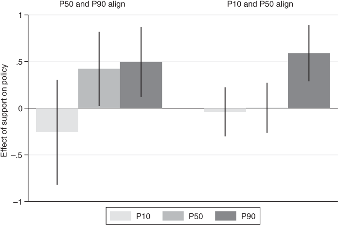
Figure 2.3 Policy responsiveness when the preferences of two groups align and the third group diverges (two-year windows)
Notes: See Table 2.A7 in the online appendix for full results. N = 115 for the left-hand panel, N = 426 for the right-hand panel.
Partisan Conditioning of Policy Responsiveness by Income
We now turn to the question of how government partisanship affects policy responsiveness. We address this question by adding measures of government partisanship to models that identify the effects of preference gaps between income groups while controlling for P50 support for policy change and interacting preference gaps with government partisanship. A negative interaction effect indicates that the pro-affluent bias in policy responsiveness becomes smaller as the presence of Left parties in government increases.Footnote 10 As we have seen (Table 2.4), preference gaps between P90 and P50 or P10 are consistently better predictors of policy adoption than preference gaps between P50 and P10 and the effects of the P90–P50 gap are quite similar to the effects of the P90–P10 gap. In light of these findings, and the pivotal role that most theories of democratic politics assign to middle-income citizens, we focus on partisan conditioning of the effects of preference gaps that involve the affluent and, especially, the gap between the preferences of high-income and middle-income citizens. In other words, the question we ask is the following: do Left (or Left-leaning) governments cater less to the high-income citizens relative to low- and middle-income citizens than non-Left (Right-leaning) governments?
Reported in Tables 2.5 and 2.6, our main results are based on measuring government partisanship as the average share of cabinet portfolios held by Social Democratic and Green parties in the year that a particular survey item was fielded and the two subsequent years.Footnote 11 As noted at the outset, Norway stands out as an exceptional case in Tables 2.5 and 2.6. In the other three countries, the effect of P90 being more supportive of policy change than P10 and P50 is positive and significant when the interaction term equals zero (indicating an absence of Left parties in government) and the coefficient of the interaction term itself is negative. It is important to note here that our Swedish sample of survey items is nearly three times as large as our German and Dutch samples, explaining why coefficients of similar magnitude for Sweden clear statistical significance thresholds while the German coefficients do not. When we pool the three countries, the coefficients for the interaction terms clear the 95 percent threshold. According to these results, pro-affluent bias in policy responsiveness is significantly less pronounced when Left parties are in power in Germany, the Netherlands, and Sweden. In Norway, by contrast, the interaction terms are positive (and significant with 95 percent confidence), suggesting that pro-affluent bias in policy responsiveness only occurs when Left parties are in power.
Table 2.5 Linear probability models interacting the P90−P10 preference gap with Left government (two-year windows)
| Pooled | Pooled (w/o NO) | Germany | Netherlands | Sweden | Norway | |
|---|---|---|---|---|---|---|
| P90−P10 gap | 0.791** | 0.898** | 1.235** | 1.058** | 0.742** | −0.125 |
| (0.122) | (0.134) | (0.297) | (0.317) | (0.138) | (0.303) | |
| Left government | −0.025 | −0.041 | −0.049 | −0.079 | −0.065+ | 0.024 |
| (0.031) | (0.038) | (0.094) | (0.165) | (0.034) | (0.052) | |
| P90−P10 × Left | −0.253 | −0.441* | −0.483 | −1.547 | −0.547** | 1.015* |
| government | (0.190) | (0.214) | (0.509) | (1.047) | (0.186) | (0.449) |
| P50 support | 0.220** | 0.170** | 0.223 | 0.284** | 0.026 | 0.353** |
| (0.049) | (0.062) | (0.156) | (0.108) | (0.049) | (0.071) | |
| Country dummies | Yes | Yes | No | No | No | No |
| Constant | 0.445** | 0.484** | 0.451** | 0.097 | 0.185** | 0.037 |
| (0.043) | (0.050) | (0.101) | (0.074) | (0.038) | (0.042) | |
| N | 1958 | 1401 | 266 | 291 | 844 | 557 |
| Adjusted R2 | 0.190 | 0.222 | 0.071 | 0.061 | 0.034 | 0.063 |
Notes: +p < 0.1, *p < 0.05, **p < 0.01.
Table 2.6 Linear probability models interacting the P90−P50 preference gap with Left government (two-year windows)
| Pooled | Pooled (w/o NO) | Germany | Netherlands | Sweden | Norway | |
|---|---|---|---|---|---|---|
| P90−P50 gap | 1.160** | 1.316** | 2.058** | 1.500** | 0.937** | −0.225 |
| (0.157) | (0.173) | (0.530) | (0.419) | (0.170) | (0.409) | |
| Left government | −0.024 | −0.040 | −0.024 | −0.141 | −0.069* | 0.025 |
| (0.032) | (0.038) | (0.090) | (0.165) | (0.032) | (0.052) | |
| P90−P50 × Left | −0.510* | −0.800** | −0.951 | −1.332 | −0.859** | 1.648* |
| government | (0.231) | (0.250) | (0.837) | (1.462) | (0.211) | (0.651) |
| P50 | 0.299** | 0.257** | 0.364* | 0.406** | 0.063 | 0.399** |
| (0.050) | (0.065) | (0.166) | (0.114) | (0.051) | (0.070) | |
| Country dummies | Yes | Yes | No | No | No | No |
| Constant | 0.406** | 0.440** | 0.366** | 0.054 | 0.163** | 0.013 |
| (0.044) | (0.051) | (0.105) | (0.074) | (0.036) | (0.041) | |
| N | 1958 | 1401 | 266 | 291 | 844 | 557 |
| Adjusted R2 | 0.190 | 0.224 | 0.067 | 0.087 | 0.038 | 0.066 |
Notes: *+p < 0.1, * p < 0.05, **p < 0.01.
Based on the results in Table 2.6, Figure 2.4 displays predicted probabilities of policy adoption at different values of the P90–P50 gap under two partisan scenarios: no Left parties in government (left-hand panel) and Left parties holding all cabinet seats (right-hand panel).Footnote 12 The Norwegian case again stands out as exceptional in this figure. Importantly, Figure 2.4 also illustrates that the Left government diminishes but does not eliminate pro-affluent bias in Germany and the Netherlands. Sweden appears to be the only case in which policy is equally responsive to high-income and middle-income citizens when Left parties control the government.

Figure 2.4 Predicted probabilities of policy change conditional on the P90−P50 preference gap and government partisanship (two-year windows)
Government Partisanship and Redistributive Policy Responsiveness by Income
The Norwegian puzzle invites further discussion of how party politics is related to income biases in political responsiveness. As noted in the introduction, our theoretical expectations regarding the impact of government partisanship apply most clearly to issues involving economic and social policies with direct distributive implications. It is much less evident that citizens’ preferences are polarized by income on the many and varied “noneconomic” (or “nonmaterial”) issues that divide Left and Right parties and, if there is polarization by income, it may well be the inverse of the polarization that we observe with issues pertaining to economic policy (in particular, fighting unemployment, taxation, and social spending). Indeed, an extensive literature on new cleavages in electoral politics argues that mainstream Left parties have sought to offset the decline of the traditional working class by aligning their programs with the preferences of “new middle strata” – relatively affluent and primarily urban voters – on environmental issues as well as immigration and a host of cultural issues encompassed by the notion of “cosmopolitanism” while seeking to retain the support of low-income voters by maintaining their commitment to redistribution of income (e.g., Gingrich and Häusermann Reference Gingrich and Häusermann2015; Kitschelt Reference Kitschelt1994; Kriesi et al. Reference Kriesi, Grande, Lachat, Dolezal, Bornschier and Frey2006). This general characterization holds for Dutch, German, and Swedish Social Democrats as well as Norwegian Social Democrats, but one might plausibly assume that the urban–rural divide is a more prominent feature of Norwegian politics – perhaps a more prominent feature of Norwegian income inequality as well – and that this has rendered the Norwegian Social Democrats, and other progressive parties with an urban base, less responsive to low-income citizens than their Dutch, German, and Swedish counterparts (Bjørklund Reference Bjørklund and Hagtvet1992; Rokkan Reference Rokkan and Dahl1966).
A detailed analysis of the issues on which Norwegian governments headed by Social Democrats have gone against the preferences of low- and middle-income citizens lies beyond the scope of this paper. We must also set aside the question of whether or not the strength of the populist Progress Party (with a vote share ranging between 14.6 percent and 22.9 percent since 2000), and its participation in government between 2014 and 2020, might have rendered Right-leaning governments more responsive to low-income citizens. What we can do to shed some light on “Norwegian exceptionalism” and, more generally, to further enhance our understanding of partisan conditioning of unequal responsiveness is to replicate the preceding analysis for a subset of survey items that pertain to economic and welfare issues. Needless to say, this involves a significant reduction in the total number of data points at our disposal and some loss of statistical power.
In assigning survey items to policy domains, we rely on the typology proposed by Kriesi et al. (Reference Kriesi, Grande, Lachat, Dolezal, Bornschier and Frey2006). The category “economic issues” thus encompasses policy questions pertaining on macroeconomic management, government regulation of the economy as well as government interventions (industrial policy), taxes, and government spending on income transfer programs as well as public services. Pooling data across the four countries, this definition of economic and welfare issues yields a sample of 681 survey items (as compared to 1,958 items for the preceding analysis).
To begin with, Table 2.7 shows the results of estimating our baseline models with preference gaps as the main independent variables (controlling for P50 support), without interacting preference gaps with government partisanship. For Germany and Sweden, these results are quite similar to the results for all survey items (shown in Table 2.4). In both of these cases, P90 preferences dominate P50 and P10 preferences. In the German case, P50 preferences also dominate P10 preferences. Although the coefficients for preference gaps are also positive for the Netherlands and Norway, none of the Norwegian coefficients clear conventional thresholds for statistical significance, suggesting that there is no systematic bias in favor of the affluent on economic issues. In the Dutch case, P90 preferences dominate P50 preferences more clearly than P10 preferences.
Table 2.7 Average marginal effects of preference gaps on policy adoption, controlling for P50 support, economic, and welfare issues only (two-year windows)
| Pooled | Germany | Netherlands | Norway | Sweden | |
|---|---|---|---|---|---|
| P90–P10 support | 0.577** | 1.010** | 0.339 | 0.157 | 0.482* |
| P90–P50 support | 0.787** | 1.563** | 0.671* | 0.338 | 0.440* |
| P50–P10 support | 0.506* | 1.422** | 0.154 | −0.268 | 0.021 |
Notes: *p < 0.05, **p < 0.01. See Tables 2.A13–15 in the online appendix for full regression results.
Turning to the conditioning effects of government partisanship, we again interact our partisanship variable (Left parties’ share of cabinet portfolios) with the P90–P50 preference gap. The results are summarized in Figure 2.5. The first thing to note is that Norway no longer stands out as an exceptional case when we restrict the analysis to economic and welfare issues. For the Netherlands and Sweden alike, Left participation in government significantly reduces pro-affluent bias in this policy domain. We do not observe such an effect for Norway, but it is no longer the case that Left participation increases unequal responsiveness. We also do not observe any significant reduction of unequal responsiveness in the German case. In short, the conventional partisan hypothesis seems to hold for the Netherlands and Sweden, but not for Germany and Norway.

Figure 2.5 Predicted probabilities of policy change, economic/welfare issues only, conditional on the P90−P50 preference gap and government partisanship (two-year windows)
Note: See Table 2.A16 in the online appendix for full regression results (and Table 2.A17 for results using the P90−P10 preference gap instead).
Changes in Policy Responsiveness by Income and Partisan Conditioning
Our German data begin in 1998, at a time when many Social Democratic parties, including the German one, had already embraced more market-friendly, less-redistributive “Third Way” policies, but our data for the other three countries extend farther back in time (to the early 1980s for the Netherlands and to the 1960s for Norway and Sweden). To explore whether the reorientation of Social Democratic parties in the 1990s entailed a decline in policy responsiveness to the preferences of low- and middle-income citizens under Left government participation, we conduct separate analyses for the period before 1998 and for the period from 1998 onwards, separating economic and welfare issues from other issues. For the P90–P50 preference gap, Figure 2.6 shows predicted probabilities of policy under the minimum Left government scenarios based on pooling survey items for all countries, that is, for three countries (the Netherlands, Norway, and Sweden) for 1960–1997 and for all four countries for 1998–2016.Footnote 13

Figure 2.6 Predicted probabilities of policy change by time period, conditional on the P90−P50 preference gap and government partisanship (two-year windows)
Note: See Table 2.A18 in the online appendix for full regression results.
Our analysis of temporal change features only pooled results for two reasons. To begin with, it goes without saying that the number of observations in country-specific analyses becomes very small when we restrict them to economic and welfare policies in one or the other subperiod.Footnote 14 Secondly, irrespective of the loss of statistical power, country-specific analyses restricted to one of these subperiods often end up comparing one or two Left-leaning governments with an equally small number of Right-leaning governments and they are arguably “contaminated” by the idiosyncratic experiences of one of these governments. We would not want to generalize about long-term changes in partisan conditioning of unequal responsiveness based on which parties happened to be in government during the Great Recession of 2008–2010.Footnote 15 Pooling data across our four countries serves to minimize the effects of such events and seems to be justified in light of the common patterns of unequal responsiveness and partisan conditioning that we have already observed.
Pooling data from all four countries, we find that Left-leaning governments were distinctly different from Right-leaning governments in the domain of economic and welfare policies prior to 1998. While the policy choices of Right-leaning governments responded primarily to the preferences of affluent citizens, Left-leaning governments were equally responsive to the preferences of low- and middle-income citizens in this policy domain. By contrast, Left-leaning and Right-leaning governments were equally biased in favor of the preferences of affluent citizens in other policy domains. Crucially for our present purposes, we no longer observe any partisan conditioning of policy responsiveness on economic and welfare issues in the post-1998 period. The pro-affluent bias of Right-leaning governments appears to have been more pronounced than in the earlier period and, at the same time, Left-leaning governments are no longer distinct from Right-leaning governments in the post-1998 period. Outside the domain of economic and welfare policies, we find that Left-leaning and Right-leaning governments were equally biased in favor of the preferences of affluent citizens in the pre-1998 period and that the pro-affluent bias of Left-leaning governments has diminished while the pro-affluent bias of Right-leaning governments has become more pronounced.
We hasten to note that the differentiation between Left-leaning and Right-leaning governments on “other issues” in the post-1998 period fails to meet standard criteria for statistical significance. The 95 percent confidence intervals overlap in two of the other panels of Figure 2.6 as well. The main take-away from the analysis summarized in Figure 2.6 is that we observe a significant effect of interacting preference gaps with government partisanship only for economic and welfare issues and only for the period prior to 1998.
Rethinking Unequal Responsiveness
Our main empirical findings can be summarized as follows. First, we find that middle-income as well as low-income citizens in Northwest Europe are consistently underrepresented compared to high-income citizens when representation is measured as responsiveness of policy outputs to stated preferences across the full range of issues captured by public opinion surveys. Second, we find that unequal responsiveness is moderated by government partisanship, such that the pro-affluent bias is less pronounced (but not zero) when Left parties are in government. The second observation comes with more qualifications than the first: it does not hold for one of our four countries (Norway) when pooling all issues, and when we separate policy domains and time periods, it applies mostly to economic and welfare issues before 1998 (possibly to noneconomic issues after 1998).
In closing, let us briefly reflect on the implications of these findings for the debates about the meaning of unequal responsiveness, as measured by Gilens (Reference Gilens2012), and the reasons why governments appear to be most responsive to the preferences of high-income citizens than to the preferences of low- and middle-income citizens. To begin with, it is truly striking that income biases in policy responsiveness, measured in this manner, are at least as pronounced in “social Europe” as in “liberal America” (Pontusson Reference Pontusson2005). How do we reconcile this observation with the fact that tax-transfer systems are significantly more redistributive in Germany, the Netherlands, Norway, and Sweden than in the United States?
As documented by Brooks and Manza (Reference Brooks and Manza2007), American citizens are, in general, less supportive of progressive taxation and redistributive social programs than Dutch, Germans, Norwegian, and Swedish citizens. This contrast holds across the income distribution and may well be more pronounced in the upper half of the income distribution. Support for redistribution among high-income citizens provides a partial explanation for the coexistence of unequal responsiveness and redistribution, but the origins of redistributive politics in Northwest Europe can hardly be explained by reference to the preferences of high-income citizens.
More plausibly, support for redistribution among high-income citizens in Northwest Europe represents an adaptation to policy developments generated by the political mobilization of low- and middle-income citizens in the wake of democratization and the Second World War. In making this argument, we think it is important to recognize that the status quo informs the policy agenda of policymakers and the questions that public opinion surveys ask as well as the way that citizens respond to these questions. And the status quo is, of course, an expression of past policy decisions. Though we lack the data necessary to test this proposition in a systematic fashion, it seems likely that policy responsiveness on economic and welfare issues, by Left-leaning and Right-leaning governments alike, was significantly more equal in Northwest Europe than in the United States in the postwar era.
Our finding that Germany, the Netherlands, and Sweden are comparable to the United States in terms of income biases in policy responsiveness in the period since the 1980s fits with the observation that German, Dutch, and Swedish governments undertook reforms that reduced the redistributive effects of taxation and government spending in the 1990s and 2000s (see Pontusson and Weisstanner, Reference Pontusson and Weisstanner2018, as well as the introductory chapter to this volume). For our present purposes, the key point is that the starting point of these developments was very different from the status quo in the United States. Consistent with this argument, perusing lists of proposed policy changes makes it quite clear that antiredistributive policy proposals are more common and more radical in Gilens’ US dataset than in our European datasets.Footnote 16
Left parties and their trade-union allies played a key agenda-setting role in Northwest Europe in the 1960s and 1970s, when redistribution became a prominent feature of tax-transfer systems in these countries. Again, our analysis yields suggestive evidence that Left-leaning governments in Northwest Europe were more responsive to low- and middle-income citizens than to the high-income citizens in the economic and welfare policy domain prior to the mid-1990s. In this respect, our findings are consistent with the long-standing literature on partisan politics as factor behind cross-national variation in the development of the welfare state.
On the other hand, these findings represent something of a challenge for the conventional view that mainstream Left parties in Northwest Europe have sought to offset the decline of the working-class constituency by appealing to middle-class voters based on new (“post-materialist”) issues while retaining the support of working-class voters based on their continued commitment to redistribution. This interpretation of the reorientation of mainstream Left parties would lead us to expect that mainstream Left parties remain “pro-poor” in the domain of economic and welfare policy while they have become more “pro-affluent” in other policy domains. Generalizing across our four countries, we find instead that mainstream Left parties, like mainstream parties of the Center-Right, have historically been biased in favor of affluent citizens outside the domain of redistributive politics and that post-1998 Left governments are first and foremost distinguished from earlier Left governments by their lack of responsiveness to low- and middle-income citizens in the domain of redistributive politics.
Setting government partisanship aside, what are the implications of our empirical findings for the debate about the causal mechanisms behind income and class biases in political representation? The “Americanist” literature identifies four plausible (and complementary) explanations for the income biases identified by Gilens (Reference Gilens2012) and others.Footnote 17 Perhaps most prominently, and most obviously, this literature posits that the costs of election campaigns and politicians’ reliance on private sources of campaign funding – what Gilens (Reference Gilens2015a: 222) refers to as the “outsize role of money in American politics” – constitute a key reason why policy outputs disproportionately correspond to the preferences of affluent citizens. A second line of argumentation in the US literature invokes the income gradient in political participation – in the first instance, in electoral turnout – to explain unequal policy responsiveness. Yet another line of argument focuses on lobbying by corporations and organized interest groups, positing either that the policy preferences of affluent citizens coincide with corporate interests to a greater extent than the policy preferences of low- and middle-income citizens or that affluent citizens are better organized and thus better represented through “extra-electoral” politics. Finally, Carnes (Reference Carnes2013) has pioneered a line of inquiry that focuses on the social and occupational backgrounds of elected representatives as the key source of unequal policy responsiveness in the United States.
As commonly noted by “Europeanists,” the fact that we also observe unequal responsiveness of a consistent and pervasive nature in countries like Germany and Sweden raises questions about the relevance of campaign finance. Surely, money matters to parties and politicians in these countries as well, but election campaigns are much less expensive and, for the most part, financed by public subsidies. The point here is not to deny that campaign finance might be an important factor in the US case, but rather to point out that other factors must be taken into account in order to explain the ubiquity of unequal responsiveness across countries. The same arguably holds for electoral participation as an explanation of unequal responsiveness. In all four of the countries analyzed in this chapter, we observe unequal turnout by income, but aggregate turnout is higher than in the United States and the income gradient is flatter. And yet overall policy responsiveness does not appear to be markedly more equal.Footnote 18
The argument about unequal responsiveness via the interest-group channel is more difficult to evaluate comparatively, but it seems reasonably clear that corporations and business associations wield less unilateral influence over elected representatives and unelected policymakers in countries with centralized policy consultations and, in particular, tripartite bodies that provide for negotiations over policy implementation as well as policy formulation between representatives of unions, employers, and governments. Our four countries all exemplify this model of “corporatist intermediation.” Especially in Norway and Sweden, unions have historically played, and continue to play, an important role as counterweights to the political influence of business actors (organized or not). Again, it is puzzling that we do not observe more equal policy responsiveness under these circumstances.
Of the various arguments invoked to explain unequal responsiveness in the United States, the argument about descriptive misrepresentation by income and social class seems most easily applied to Northwest Europe. Elected representatives in Germany, the Netherlands, Norway, and Sweden are less likely to be multimillionaires than their American counterparts, but they come overwhelmingly from the ranks of university-educated professionals and tend to belong to the top two or three deciles of the income distribution (see Carnes and Lupu’s contribution to this volume). A growing number of studies show that occupational background and associated life circumstances and social networks influence the policy preferences and priorities of elected officials across a wide range of different national contexts (Alexiadou Reference Alexiadou2022; Carnes and Lupu Reference Carnes and Lupu2015; Hemingway Reference Hemingway2020; O’Grady Reference O’Grady2019; Persson Reference Persson2021; Curto-Grau and Gallego in this volume). In a related vein, recent studies find that elected representatives tend to be more accurate in their perceptions of the preferences of affluent citizens than in the perceptions of the preferences of poor citizens (Pereira Reference Pereira2021; Sevenans et al. Reference Sevenans, Marié, Soontjens, Walgrave, Breunig and Vliegenthart2020). Arguably, this line of argumentation is particularly relevant for understanding the reorientation of mainstream Left parties, as the social backgrounds of candidates for public office fielded by these parties at the national level have become more like those of candidates fielded by other mainstream parties over the last two or three decades.
Beyond these four possible mechanisms, a number of alternatives ought to be considered. In addition to factors pertaining to the behavior of citizens and political elites, the unequal policy responsiveness that we observe across many countries might plausibly be attributed to the systemic power of capital. Following Block (Reference Block1977), the argument would be that governing parties are not responding to any specific demands placed on them by citizens or interest groups, but rather seeking to maximize their chances of reelection by incentivizing capital owners (private individuals) to invest and thereby improve macroeconomic performance. A crucial additional step in the argument would be that the policy preferences of high-income citizens tend to be more closely aligned with the interests of capital owners than the preferences of low- and middle-income citizens. For our present purposes, suffice it to note that this line of argument would seem to imply that unequal responsiveness should be most pronounced with regard to policy issues that bear directly on the interests of capital owners (and conflicts of interest between capital and labor). In other words, we should observe greater pro-affluent bias in the domain of economic and welfare policies than in other policy domains. Our analysis does not yield any evidence in support of this expectation.
Articulated by Persson (Reference Persson2023), another argument that might explain the ubiquity of unequal responsiveness concerns status-quo bias. Simply put, this argument posits that low-income citizens are less satisfied with the status-quo than high-income citizens and, as a result, more likely to support policy changes in general. To the extent that this is true, and given the way that we measure policy outcomes, status-quo bias produces policy outcomes that look as if policymakers were responding disproportionately to the demands of affluent citizens. Analyzing the Swedish dataset on which we draw for this paper, Persson (Reference Persson2023) shows that income groups have had very similar preferences with regard to policy changes that have been adopted, but low-income citizens have been much more supportive of policy changes that have not been adopted than affluent citizens (with middle-income support very much in the middle). As shown in Table 2.2, however, we observe little or no difference between income groups in their average support for policy changes in Germany, the Netherlands, and Norway.Footnote 19
Related to status-quo bias, there is an alternative interpretation of the evidence for unequal policy responsiveness presented earlier that we ought to engage with in a more systematic way than scholars working in this domain have done so far. Observing that policy change happens more often when it is supported by affluent citizens and that support by citizens in the lower half of the income distribution has little, if any, effect on the probability of policy adoption, it is commonplace to conclude that politicians listen to affluent citizens more than they listen to low- and middle-income citizens. But perhaps it is the other way around. Perhaps it is the case that affluent citizens listen more to politicians than low- and middle-income citizens do. We know that income and education are closely correlated and many studies demonstrate that more educated citizens are more interested in and knowledgeable about politics (e.g., Schlozman, Verba, and Brady Reference Schlozman, Verba and Brady2012). Arguably, this means that affluent citizens are more likely to take their cues from policymakers (or debate among “insiders”) in deciding whether they favor or oppose specific policy proposals. More specifically, it seems quite plausible to suppose that more “sophisticated” citizens are more likely to rule out policy options that are unrealistic in the sense that they are unlikely to be entertained by policymakers.Footnote 20
Our empirical findings concerning partisan conditioning of unequal responsiveness raise questions about the reverse-causality line of argument. For the period prior to 1998, our results indicate that Left governments were more responsive to the preferences of low- and middle-income preferences in the domain of economic and welfare policies, but they were more responsive to high-income preferences in other policy domains. Simply put, why should the affluent (well-educated) adapt their preferences to elite discourses under some governments but not others and in some policy domains but not others? And why did low-income citizens apparently take cues from Left governments prior to the 1990s, but not thereafter? When all is said and done, the evidence on partisan conditioning presented in this paper suggests that unequal policy responsiveness to the preferences of different income groups does capture something important about the distribution of political influence in Northwest Europe as well as the United States. Yet much research remains to be done in order to explain the ubiquity of unequal policy responsiveness as well as variation in responsiveness across time, policy domains, and countries.
A long line of work on advanced capitalist democracies argues that the need for governments to assemble majority electoral coalitions accords the middle class a strong say over government policies and virtually ensures that it will share in the prosperity that modern capitalism enables (e.g., Baldwin Reference Baldwin1990; Esping-Andersen Reference Esping-Andersen1990; Iversen and Soskice Reference Iversen and Soskice2006; Korpi and Palme Reference Korpi and Palme1998; Meltzer and Richard Reference Meltzer and Richard1981; Rothstein Reference Rothstein1998). Such sharing takes many forms, but the two main vehicles are investments in skills and the welfare state (Huber and Stephens Reference Huber and Stephens2001; Iversen and Stephens Reference Iversen and Stephens2008). Recent work, however, including several contributions to this volume, call the conventional wisdom into doubt. One line of research argues that policies are strongly biased toward the preferences of the rich, as revealed in public opinion surveys (e.g., Bartels Reference Bartels2008, Reference Bartels2017; Gilens Reference Gilens2005, Reference Gilens2012; Gilens and Page Reference Gilens and Page2014); another argues that the structural power of increasingly footloose capital undermines the capacity of the state to tax and redistribute rendering democratic governments increasingly incapable of responding to majority preferences (e.g., Piketty Reference Piketty2014; Rodrik Reference Rodrik1997, Reference Rodrik2011; Streeck Reference Streeck2011, Reference Streeck2016). This chapter is a critical reassessment of these and related arguments using macro evidence on government taxation and spending. Without probing preferences directly, we ask which classes gain and lose from government policies, and whether such “revealed power” has changed over time. We base our estimates on LIS data amended by data on in-kind government spending and we complement this evidence with data from the new World Inequality Database (WID). In a separate paper, we have examined evidence on preferences based on ISSP data (Elkjær and Iversen Reference Elkjær and Iversen2020).
Broadly consistent with the older literature, we find that government policies and outcomes in most cases are responsive to the economic interests of the middle class, and we show that middle-class power over fiscal policies has remained remarkably stable over time, even though market inequality has risen sharply and despite a large recent literature on the “hollowing-out of the middle.” The rich are as large net contributors to the welfare state today as they were in the past, and it does not appear that the democratic state is increasingly constrained by global capital. In most cases, the middle class, measured by posttax income, has kept up with the advancement of the economy as a whole. The partial exception is the United States where middle-income growth has lagged average growth, although in absolute terms posttax incomes rose at a comparable rate to Europe.
Perhaps surprisingly, these conclusions appear to also apply to the bottom end of the income distribution. Growth in the posttax incomes of the bottom income quintile largely follows average incomes, although here the United States is an even greater outlier with bottom-end inequality rising sharply. We find that the bottom benefits from center-left governments, but the capacity of the bottom to keep up with the middle seems to be mainly driven by demand for insurance and public goods in the middle class.Footnote 1 In this sense, the poor are highly vulnerable, even under democracy, since they depend on the middle class defining its interests as being bound up with those of the poor. There are reasons to think this may be less true today than in the past.
Our comparison of the LIS data, which is based on equivalized household income, and the WID data, which is based on individualized income, reveals the important role of the family in shaping distributive outcomes. There is much redistribution going on within the household because members share consumption (notably living space, food, and consumer durables), but lower marriage rates and rising divorce rates have created many more single-adult households, which affect both distributive outcomes and distributive politics. Interestingly, this trend has produced very different outcomes in Europe and the United States, and it seems to be bound up in part with the role of race in US politics.
As Lupu and Pontusson note in their introduction, our overall findings appear at odds with theirs. We agree that one reason is that our data are for a longer period and for a larger sample of countries. It also matters that we include in-kind transfers in our analysis, while they do not. Lupu and Pontusson note that the distribution of these transfers depends on assumptions that cannot be fully validated with current data. Yet excluding in-kind transfers implicitly assumes that they are proportional to after-tax income, which is almost certainly not the case, so that is not a solution. Still, if we do exclude in-kind transfers, it does not much affect the trends we document over time (our focus) since the magnitude and composition of in-kind transfers do not change much. We should also note that our results are substantively identical whether we exclude students and retirees from the analysis or exclude people without factor income. Finally, while we agree that transfer rates are not the only test of models of redistributive politics, a remarkable implication of our results is that the evolution of transfer rates – which we use as a signal of political power – produces largely constant relative post-fisc incomes over time for the middle and bottom. This is not an accounting relationship, as Lupu and Pontusson’s hypothetical example in the introduction illustrates, and it is consistent with rising inequality in the top half.
The rest of the chapter is organized into three sections. The first is a critical assessment of the state of the literature, comparing recent arguments about the subversion of democracy to more long-standing theories of the pivotal role of the middle class. We offer definitions of class interests over government tax-and-spend policies, and we hypothesize different patterns of spending priorities depending on class power. We then turn to the empirics, showing evidence from eighteen advanced democracies going back to the 1970s, with a focus on how different classes have fared over time according to both LIS and WID data. The last section concludes.
Theoretical Perspectives
The Subversion of Democracy Debate
In recent decades, a deep pessimism about advanced democracy and its capacity to serve the needs of ordinary people has taken hold. It is not hard to find reasons to be concerned: rightwing populism, rising inequality, declining growth, and a concentration of wealth that leaves the impression that the system increasingly works only for the rich and powerful. There is worrying evidence to back up such pessimism. Work by Bartels (Reference Bartels2008), Gilens (Reference Gilens2005, Reference Gilens2012), and Gilens and Page (Reference Gilens and Page2014) on the US, as well as recent work testing and extending their approach to other advanced democracies (e.g., Bartels Reference Bartels2017; Elsässer, Hense, and Schäfer Reference Elsässer, Hense and Schäfer2018; Peters and Ensink Reference Peters and Ensink2015; contributions to this volume) find that the affluent dominate democratic politics to the point where other income classes do not matter. This is of obvious normative concern, and it also challenges standard models of democracy, which accord a strong role to the middle class.
Yet, the interpretation of the public opinion evidence is contested (see e.g., Elkjær and Klitgaard Reference Elkjær and Klitgaard2021). Subgroup preferences are highly correlated over time (Page and Shapiro Reference Page and Shapiro1992; Soroka and Wlezien Reference Soroka and Wlezien2008), and the middle class emerges as far more politically influential when preferred levels of spending are used instead of preferred changes in spending (Elkjær and Iversen Reference Elkjær and Iversen2020). Nor do public opinion data capture the role of political parties. Voters may be generally uninformed about politics, which shows up as noisy survey responses and ill-considered policy positions, but they may know enough to vote for parties that are broadly representative of their interests, using either ideological cues (as originally argued by Downs Reference Downs1957) or retrospective economic evaluations (Fiorina Reference Fiorina1981; Kitschelt Reference Kitschelt2000; Munger and Hinich Reference Munger and Hinich1994). Political parties may thus act as “trustees” for their constituencies and advance their long-term interests in government; what Mansbridge (Reference Mansbridge2003) calls “promissory representation.” Most plausibly, effective representation requires parties to pay attention to both interests and preferences, as argued long ago by Pitkin (Reference Pitkin1967). For this reason, evidence on expressed preferences as well as interests is salient for assessing power and influence.
In his contribution to this volume, Bartels criticizes some of this and our other earlier work, arguing that we assign undue importance to bivariate associations of policies and preferences. In reality, though, we follow a line of scholarship dating back to at least Nagel (Reference Nagel1975), who distinguished between the ‘influence’ an actor exerts on an outcome and the “benefit” they receive from their own and others’ influence. The latter, Nagel (Reference Nagel1975: 156–7) argued, can be measured as the correlation between preferences and the outcome. In practical terms and considering the strong model dependency of published results (Elkjær and Klitgaard Reference Elkjær and Klitgaard2021), we also think it’s ill-advised to ignore the bivariate associations. In the face of even minor model misspecifications, the high levels of multicollinearity that are inherent in multivariate models of preferences and political outcomes might thus greatly exacerbate statistical bias (see Winship and Western Reference Winship and Western2016). Finally, and perhaps most importantly, Bartels’ critique has no bearing on our substantive conclusions: when we use Bartels’ preferred specification, the middle class still stands out as a pivotal player in redistributive politics (some of these results are presented in appendices to the original papers).
Even if governments respond to middle-class electorates, however, these responses may be increasingly constrained and inadequate. New work in comparative political economy highlights macro trends that appear to show that governments do not respond to rising inequality – a puzzle that is known as the Robin Hood paradox (following Lindert Reference Lindert2004). In addition, there is evidence that partisanship matters less for government policies than in the past (Huber and Stephens Reference Huber and Stephens2001; Kwon and Pontusson Reference Kwon and Pontusson2010). Such “convergence” could reflect that governments are increasingly hamstrung by footloose capital, as argued by Streeck (Reference Streeck2011, Reference Streeck2016), Piketty (Reference Piketty2014), and Rodrik (Reference Rodrik1997, Reference Rodrik2011). Closely related, businesses and high-income earners may have the ability to shift their consumption, income, and effort to offset higher taxes, which places a binding constraint on how much governments can tax. Rising top-end incomes would incentivize the rich to engage in additional tax shifting. Another possibility is that big business and the rich exert political influence behind the scenes, outside the light of public discourse and open electoral contests (Hacker and Pierson Reference Hacker and Pierson2010; Hertel-Fernandez Reference Hertel-Fernandez2018, Reference Hertel-Fernandez2019; Rahman and Thelen Reference Rahman and Thelen2019).
On the other side of the debate are arguments about the geospatial embeddedness of advanced capitalism. As argued by economic geographers (e.g., Glaeser Reference Glaeser2011; Storper Reference Storper1997, Reference Storper2013) and business scholars (e.g., Iammarino and McCann Reference Iammarino and McCann2013; Rugman Reference Rugman2012), advanced production is rooted in local skill clusters, which tend to be concentrated in the successful cities, and these clusters are complemented by dense colocated social networks, which are very hard to uproot and move elsewhere (Iversen and Soskice Reference Iversen and Soskice2019). In this perspective, trade and foreign investment tend to reinforce local specialization and raise the dependence of multinational capital on location cospecific assets, most importantly highly skilled labor, and the mostly tacit knowledge they represent. This makes sustained tax evasion through mobility or income shifting hard. Intense market competition, especially in globalized markets, also makes it hard for business to coordinate politically. From this perspective, globalization does not undermine the capacity of governments to respond to democratic demands and may in fact augment it.
Class Interests
In this chapter, we abstract from public opinion data and instead use an axiomatic approach where class interests are derived deductively and then compared to actual tax-and-spend policies over time.Footnote 2 This offers partial evidence on class power. As noted earlier, a fuller picture would also require attention to preferences. We have done so in a separate paper (Elkjær and Iversen Reference Elkjær and Iversen2020). The assumptions and mathematical derivations for our predictions are relegated to Appendix 3.A; here we focus on the key intuitions. The baseline model predicts patterns of taxation and spending, but our empirical approach does not presuppose any particular channel of influence, or whether voters are informed or not, or whether governments have high capacity or not. Deviations from the baseline predictions will instead alert us to potential violations of assumptions, which invite alternative interpretations.
As in much work before ours, we divide the adult population into three income classes: low (L), middle (M), and high (H). We assume that each class is only concerned with maximizing its own material welfare. Altruism, racial animosity, and moral reasoning are all ignored for the purpose of parsimony and clear predictions, but we will consider some of these alternative motivations in the discussion of the evidence.
Fiscal policies are characterized along three dimensions, which reflect the main material concerns of each class: (i) maximize net income; (ii) optimize social insurance, and (iii) optimize the provision of public goods. In the case of M, net income is maximized by taxing H and transferring the proceeds to M, subject to a standard cost of taxation, which is rising exponentially in the tax rate because of multiplying work and investment disincentives, rising administrative costs of enforcing tax rules, etc. Optimal taxation of H will stop well short of confiscatory taxation for these reasons.Footnote 3 This approach follows a long “optimal taxation” tradition going back to Mirrlees (Reference Mirrlees1971) and also employed by Meltzer and Richard (Reference Meltzer and Richard1981).
A somewhat different approach focuses not on what is the optimal tax rate, but instead on what is feasible. Known as the New Tax Responsiveness literature (Feldstein Reference Feldstein1995, Reference Feldstein1999; Gruber and Saez Reference Gruber and Saez2002; Saez, Slemrod, and Giertz Reference Saez, Slemrod and Giertz2012), the focus is on the capacity of businesses and high-income earners to shift their consumption, income, and effort to offset higher taxes, which places a binding constraint on how much governments can tax. Higher taxes essentially induce a substitution effect into lower-taxed income streams. An unambiguous implication of the New Tax Responsiveness literature is that rising top-end incomes incentivize the rich to engage in more tax shifting, and it therefore ties into the broader argument about inequality and class power used in this volume. In this formulation, for M to retain its political influence and keep up taxation of H during periods of rising top-end inequality, it must counter not only the “instrumental power” of the rich to shape the tax structure but also their “structural power” to evade taxation within any given tax structure. With rising top-end inequality governments must continuously find new ways to plug tax loopholes and dissuade tax evasion. In this version, the difference between a constant and a falling H transfer rate is the difference between a politically resilient nonrich majority and an ascending rich minority.
In a changing world, governments need to continuously update their tax regimes to address demands from the middle class. This is also true on the spending side. Demand has shifted away from traditional social consumption toward social investment (Garritzmann, Hausermann, and Palier Reference Garritzmann, Häusermann and Palier2022). It is precisely because the content of policies is changing all the time that a theory of class power cannot rely entirely on arguments about path dependence (Pierson Reference Pierson1996; 2000). The focus of our analysis is the capacity of the lower and (especially) the middle classes to continuously reinvent tax and spend policies to satisfy their material interests. Our argument is not about the stasis of policy, but about the resilience of class power.
We start by defining what we will refer to as transfer rates for each class:

where,  refers to each of the three classes, i = {L, M, H}. We measure transfer rates relative to net (after-tax and transfer) income because it is readily observable whereas we cannot observe market income in the counter-factual case of zero taxation. A positive number means that a group is a net beneficiary; a negative number that it is a net contributor.
In Appendix 3.A, we first show that if M is pivotal, optimal taxation implies a constant transfer rate from H:

where the superscript indicates that this is M’s preferred rate for H. If M chooses the optimal rate, there is no relationship between top-end inequality and redistribution.Footnote 4 The reason is that higher income of H always compensates M optimally through higher transfers, without changing the rate at which H is taxed. Note, however, that H will pay more into the public purse and M will consequently see transfers rise as a share of its own income, as H’s relative income rises:

This prediction stands in contrast to arguments that the rich enjoy increasing influence over policies as they become richer. If that was true, H’s and M’s transfer rates should fall as high-end inequality rises.
In the New Tax Responsiveness approach, the H-transfer rate is a direct measure of the power to tax high incomes, but unlike the optimal taxation approach, it does not make any predictions about how the transfer rate changes in response to top-end inequality. This will depend on the capacity of the rich to find ways to shift income to lower-taxed assets versus the capacity, administrative and political, of the state to close such opportunities. In this formulation, a constant H transfer rate is an expression of constant middle-class power, but the prediction of a constant transfer rate follows only from complementary arguments about democracy and the power to tax, which we reviewed earlier.
Social insurance follows a distinct logic. M may well want to spend money on social insurance, which we can think of as guarantees against the risk of losing income and falling into the L group. This could be because of unemployment, illness, or just bad luck (such as being in an industry or profession facing falling demand and wages). Those with high incomes tend to be less exposed to such risks (Moene and Wallerstein Reference Moene and Wallerstein2001; Rehm Reference Rehm2011), and they also tend to have better access to private insurance (Busemeyer and Iversen Reference Busemeyer and Iversen2020). For M, on the other hand, insurance against labor market and other social risks is usually seen as a critically important motive for supporting public spending, and it has been documented to matter greatly in historical accounts (Baldwin’s Reference Baldwin1990; Esping-Andersen Reference Esping-Andersen1990; Mares Reference Mares2003); it is implied by economic models (Barr Reference Barr2001, Reference Barr2012; Boadway and Keen Reference Boadway, Keen, Atkinson and Bourguignon2000); and it has been shown to matter for government spending and demand for such spending (Iversen and Soskice Reference Iversen and Soskice2001; Moene and Wallerstein Reference Moene and Wallerstein2001; Rehm Reference Rehm2011). This may be particularly true in an intergenerational perspective, where health insurance and old-age care help alleviate worries about older parents and where concerns about downward mobility of children give cause to support policies that ensure a decent living even for those at the bottom.
Because the demand for social insurance is proportional to risk times the loss if that risk is realized, bottom-end inequality should increase the transfer rate for L (see Appendix 3.A, eq. A6):

In the Lupu-Pontusson (Reference Lupu and Pontusson2011) model, low-end inequality instead increases “social distance,” which undermines the solidarity or affinity M feels with L. Since this is not a strictly material incentive, it is outside our model and both motives could matter. In the end, it is therefore an empirical matter.
Preferences for public goods should follow a very similar pattern because L (and H) share in spending on in-kind goods, such as infrastructure, primary and secondary schooling, policing, postal services, and so on, which are typically guaranteed as a citizen right. No person will be required to show proof of income to be admitted to, say, the local school or public library. If utility for such goods is concave, the demand function will look very similar to that for insurance, and for some in-kind services like hospitals, the distinction between insurance and public goods is blurred (see Busemeyer and Iversen Reference Busemeyer and Iversen2020).
Our focus has been on the policy interests of M because of the centrality of the middle class in standard arguments about the welfare state. But we have implicitly assumed the interests of L and H, and they can be easily summarized: L would want to tax M and H at the maximum rate and transfer everything to L; H would want to cut taxes and transfers to zero, or perhaps a positive but low number that reflects its demand for public goods and social insurance that cannot be purchased in the private market (the private market is preferable for H because it involves no redistribution).
If M cannot govern alone, the outcome will reflect a coalition bargain, which can be conceived as a policy vector of taxes and transfers to and from each class based on the above set of interests. Because the interests of L and H are diametrically opposed, it stands to reason that LH coalitions are rare. For the two other feasible coalitions, an LM coalition is expected to benefit L more, and hurt H more, than an MH coalition. Depending on bargaining power within the coalition, which we approximate in the empirical analysis as the share of right cabinet seats minus the share of left cabinet seats, M can ordinarily ensure that it will emerge as a net beneficiary. Of course, this is also ultimately an empirical matter.
As is true for the pure M model, government partisanship only matters if the power of democratic governments is not subverted by money or by the structural power of capital. If H is powerful, despite not being a majority, it will be reflected in a lower (absolute) H transfer rate. We have already suggested that if “money talks” in politics, we should expect rising upper-end inequality to be associated with lower transfer rates to M and L. The same is true if rising incomes at the top lead to more tax shifting, which is not counter-balanced by government revisions of the tax code. The argument that mobile capital undermines redistribution is readily captured in the optimal taxation model as an increase in the efficiency costs of taxation (alpha in the formal representation in Appendix 3.A). If capital moves offshore in response to higher taxation, it reduces the optimal tax rate:
 .
.In the embedded capitalism interpretation, which implies that the state is strong, neither rising inequality nor increasing globalization of capital should affect the transfer rate to M.
Empirics
Estimating Equation
We can put our hypotheses to a test using a simple encompassing regression model, where the transfer rate to M (measured either relative to H’s or M’s income) is the dependent variable:

where the first two terms measure the direct effects of relative income on the transfer rate to M; Mobility refers to widely used measures of the internationalization of capital; and Government partisanship captures the relative influence of Right versus Left parties in government (measured by cabinet shares). The relative income of M to L is included to test for social insurance motives for spending at the bottom.
Data
For the main part of the analysis, we use a new dataset that relies on household income data from the Luxembourg Income Study (LIS), supplemented by OECD and Eurostat data on spending on services and transfers, taxation of property, capital, and consumption. LIS provides a cross-national database of harmonized household income surveys going back to the 1970s. We restrict our sample to eighteen advanced democraciesFootnote 5 for which data are recorded at more than one point in time between 1974 and 2016, and we confine the sample to households that have positive market and disposable incomes. Market income inequality and transfers are greatly exaggerated when including nonworking households, the far majority of which are retirees. This is particularly true of countries with generous public pension benefits, where many do not save for their old age and will therefore appear as “poor” (Huber and Stephens Reference Huber and Stephens2001). Another sizable group is students, who we would not ordinarily think of as poor since they have high expected future income.
We measure market income as the sum of labor, cash, and capital income plus private transfers, and disposable income as total cash income minus income taxes and social contributions. Following LIS standards, market and disposable incomes are equivalized by the square root of the number of household members, and they are bottom- and top-coded at one percent of the mean equivalized income and ten times the median unequivalized income. We use market income to calculate inequality indices and divide households into deciles.
The LIS household income surveys account for cash transfers but not for in-kind services (public goods in the theoretical discussion). To include the value of services, we rely on estimates of the combined value of education, healthcare, social housing, elderly care, and early childhood education and care. The estimates are from the OECD/EU database on the distributional impact of in-kind services and are, to the best of our knowledge, the only available data (OECD 2011: Ch. 8). We also rely on an allocation key from this database to distribute the gross value of services to each income decile’s disposable cash income.Footnote 6 The exact procedure we used is explained in Appendix 3.B.
Before estimating the transfer rate, we allocate the costs of transfers and services to the income deciles’ disposable income. Transfers and services are financed by tax revenues that mainly come from taxation of income, capital, property, and consumption. The LIS data capture the income tax burden of each income decile. Business taxes are treated as neutral with respect to income classes and simply added to government revenues. The rest is financed by (i) property and wealth taxes, which are paid almost exclusively by those in the top few percentiles and therefore added to the tax burden of the top income decile, and (ii) consumption taxes, which we assume are paid in proportion to each income decile’s consumption share. Further details are provided in Appendix 3.B.
The sum of disposable cash income and the net value of in-kind services is called the net “extended” income of each income decile. Subtracting market income from net extended income yields net transfers received. Following the theoretical expectations discussed earlier, the rate of transfers to M is net transfers received by the 5th income decile divided by the net extended income of the top income decile. To account for the value of insurance, we add (in some models) the transfer rate to L weighted by the sum of the unemployment and involuntary part-time employment rates (the mean weight is .1).Footnote 7 We also calculate transfer rates for all three groups expressed as a share of their own net extended income and use these as dependent variables in some models.
Variation in Transfer Rates
Figure 3.1 shows net transfers to M as a share of the net extended income of H (top panel) and M (bottom panel) with and without accounting for insurance (left and right panels). The gray lines are country-specific local polynomial smoothers and the black line describes the entire sample of countries and years.
Figure 3.1 Net transfers to M as a share of the net extended income of H and M
Notes: N = 110. The figure shows net transfers to M as a share of the net extended income of H (top panel) and M (bottom panel) excluding and including the value of social insurance (left and right panels). The grey lines are country-specific local polynomial smoothers and the black line describes the entire sample of countries and years.
The panels illustrate that there is considerable spatial variation in the rate of transfers to M. The highest average values are observed in Ireland, Luxembourg, and Sweden and the lowest in the Netherlands and Germany. The average transfer rate to M is .05, ranging from –.06 in the Netherlands in 1993 to .14 in Ireland in 2010 (top left panel). The negative values imply that the 5th income decile is a net contributor to spending in a few country years. That is the case in Germany in the 1990s, in Netherlands in the 1990s and 2000s, and in Australia in 1981.
Accounting for insurance increases the rate of transfers to M on average by .022 and makes the 5th income decile a net beneficiary of spending in Germany already in the mid-1990s and in the Netherlands in the mid-2000s (top right panel). However, we may significantly underestimate the value of insurance. The calculation is based on the twin assumptions that people are mildly risk-averse (RRA = 1) and that the risk of falling into the L group is equal to the rate of unemployment and underemployment.Footnote 8 If people are more risk-averse (as empirical estimates suggest), if there are risks of falling into the L group for other reasons (such as illness or divorce), or if concerns about downward intergenerational mobility matter, the value of insurance will increase. More accurately accounting for the value of insurance is an important task for future research. Our substantive results are robust to increasing the weight of L’s transfer rate all the way to 50 percent (models are reported in Table 3.C1 in Appendix 3.C).
The lower panels show that transfers and services account for a substantial part of M’s extended income. On average, 9.3 percent of M’s extended income comes from transfers and services, topping at 25 percent in Ireland in 2010. Adding the value of insurance increases the average to 16 percent, with a maximum of 44.1 percent in Spain in 2013.
Turning to the trends in the top panel of Figure 3.1, we see that during the last forty years, a period of sharply rising inequality, the rate of transfers to M has been remarkably stable if not slightly increasing. This is consistent with (H1) and suggests that M’s transfer rate is unrelated to the relative income of H to M. It serves as a first indication that increased inequality has not weakened the power of the middle class to tax and redistribute income from the rich. Given that the rate of transfers from H to M is stable, it follows directly that net transfers to M have increased over time when expressed as a share of M’s own extended income. This is shown in the bottom panels of Figure 3.1, and it corroborates (H2).Footnote 9
In Figure 3.2, we show net transfer rates for all ten income deciles (net transfers for each decile as a share of the net income of H). We only show period averages (for 2010) because the rates are very stable over time, with only a slight increase in the transfer from the top decile to the other groups. What stands out is the overall redistributive effect of the tax and spending system (including transfers and public services) and the extent to which those in the top decile are net contributors. One might infer that the bottom end are the greatest beneficiaries, but it must again be kept in mind that if public spending serves insurance purposes, bottom-end transfers are also benefits for the middle. The overall picture that emerges is consistent with standard arguments about the redistributive effects of democracy, and there is no hint that the rich can skirt contributing to the system or that they are better able to do so today than fifty years ago.Footnote 10
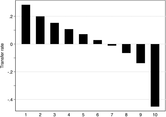
Figure 3.2 Net transfers by income decile
What Drives Transfers to and from Different Classes?
To put the descriptive results to a stricter test, we regress in Table 3.1 the rate of transfers to M on market income inequality, capital mobility, and partisanship of the government (using the previous estimating equation). Capital mobility is measured by Chinn and Ito’s (Reference Chinn and Ito2006, Reference Chinn and Ito2008) capital account openness variable and we also include trade openness as a measure of globalization (it is the sum of imports and exports as a share of GDP).Footnote 11 Partisanship of the government is a twenty-year moving average of the share of government-controlled parliamentary seats held by Right parties minus the share of government-controlled seats held by Left parties (based on Armingeon et al. Reference Armingeon, Wenger, Wiedemeier, Isler, Knöpfel, Weisstanner and Engler2018).Footnote 12 In addition, we include controls for labor force participation rates, unemployment, and real GDP growth.
Table 3.1 Determinants of net transfers to M as a percentage of H’s net income
| (1) | (2) | (3) | (4) | |
|---|---|---|---|---|
| Transfer rate M (%) | Transfer rate M incl. insurance (%) | |||
| P90/P50 | 0.84 | 2.62 | 0.26 | 1.99 |
| (3.33) | (4.16) | (3.29) | (4.07) | |
| P50/P10 | 1.79* | 1.34+ | 2.59* | 2.23* |
| (0.78) | (0.76) | (0.70) | (0.75) | |
| Trade openness (ln) | 2.40 | 0.71 | 1.82 | 0.61 |
| (1.93) | (2.79) | (1.93) | (2.80) | |
| Capital market openness | 1.16 | 2.04 | 0.22 | 1.03 |
| (2.21) | (2.10) | (1.93) | (2.03) | |
| Government partisanship (right) | −4.31* (1.46) | −3.67* (1.06) | −4.58* (1.55) | −4.07* (1.24) |
| Labor force participation | −0.23+ | −0.14 | −0.27* | −0.20 |
| (0.12) | (0.13) | (0.11) | (0.12) | |
| Unemployment | −0.05 | −0.02 | 0.15 | 0.16 |
| (0.14) | (0.12) | (0.11) | (0.10) | |
| Real GDP growth | −0.21 | −0.12 | −0.20 | −0.13 |
| (0.14) | (0.11) | (0.14) | (0.12) | |
| Trend | −0.27 | −0.22 | ||
| (0.19) | (0.20) | |||
| Trend2 | 0.01 | 0.00 | ||
| (0.00) | (0.00) | |||
| Constant | 3.66 | 3.33 | 9.53 | 7.77 |
| (9.01) | (18.23) | (8.58) | (17.78) | |
| R-squared | 0.38 | 0.42 | 0.49 | 0.52 |
| N | 110 | 110 | 110 | 110 |
Notes: *p < 0.05, +p < 0.1. Standard errors clustered by country in parentheses. All models include country fixed effects.
The results of Table 3.1 show that there is no association between top-end market income inequality and the rate of transfers to the middle class, providing further supportive evidence of (H1). In fact, the coefficients are positive, although they are always insignificant. The coefficients are also positive, and significant, for bottom-end inequality (the P50/P10 ratio). It is tempting to interpret this result from a Lupu-Pontusson (Reference Lupu and Pontusson2011) perspective to imply that a greater economic “distance” to the poor causes more resources to be concentrated in the middle. Yet, we will see later that the P50/P10 ratio is also positively related to L’s transfer rate (the skew has no effect). It appears that a middle class with a higher relative position in the income distribution has more political clout to redistribute to itself, which also brings L up in the process. Perhaps a higher P50/P10 ratio signals a more educated and politically efficacious middle class, but this is speculation – we do not know the mechanisms behind this effect. It stands up to a variety of controls, so it is not the result of any obvious omitted variable bias.
Capital mobility, whether measured by capital account openness or trade openness, has no impact on the rate of transfers to the middle class. The most obvious interpretation is that trade and foreign direct investment do not undermine, and may reinforce, specialized local knowledge clusters, which are not themselves mobile and therefore leave the state in a position to tax. Nothing in our data suggests that globalization has undermined the position of the middle class, which is consistent with (H4).
Instead, distributive politics seems to depend strongly on partisanship. In model (1), the coefficient for partisanship of the government suggests that stronger Left party participation in government is associated with higher rates of transfers to the middle class. And the size of the effect is substantial. A one standard deviation increase in left (right) partisanship of the government is associated with a 0.74 percentage points increase (decrease) in the rate of transfers to M.
In model (2), we add a time trend to the specification to ensure that our results are not driven by temporal trends. The results are robust to this alternative specification. The time-trend variables themselves are also not indicating any significant decline in transfer rates over time, as would be expected if governments were increasingly limited by capital mobility (in case these are not fully captured by the Chinn and Ito or the trade measures) or by new high-income veto players.
In models (3) and (4), we include insurance as part of the transfer rate to M. Overall, the results are very similar to those of models (1) and (2). Top-end inequality and capital mobility are not related to the transfer rate, while bottom-end inequality is. The effect size of partisanship remains stable. All in all, accounting for insurance increases the transfer rate to the middle class but the associations between the transfer rate, inequality, capital mobility, and government partisanship remain stable.
In Table 3.2, we show the results for the rate of transfers to L and to H, defined as the bottom and top deciles, respectively. For L, the results largely mirror those for M: there is little-to-no effect of top-end inequality, of capital openness, or of trade whereas left partisanship and bottom-end inequality increase transfers, as expected. For partisanship, a one standard deviation increase in right (left) partisanship decreases (increases) the transfer rate to L by 0.5 percentage points. For the P50/P10 ratio, a one standard deviation increase raises transfers to L substantially by 5.5 percent of L’s net income. It appears that as the distance between L and M increases, M becomes increasingly concerned about the risk of downward mobility and therefore supports more transfers to L. This result is consistent with (H3).
Table 3.2 Determinants of net transfers to L and H as a percentage of own net income
| (1) | (2) | (3) | (4) | |
|---|---|---|---|---|
| Transfer rate L (%) | Transfer rate H (%) | |||
| P90/P50 | −6.07 | −13.69+ | −20.00+ | −15.50 |
| (5.03) | (7.67) | (10.17) | (14.29) | |
| P50/P10 | 9.11* | 9.47* | −2.56 | −2.22 |
| (1.40) | (1.36) | (2.34) | (2.54) | |
| Trade openness (ln) | 5.06 | 3.03 | 14.92* | 19.41* |
| (3.68) | (3.36) | (6.57) | (8.02) | |
| Capital market openness | 7.44+ | 4.54 | 12.66 | 14.07 |
| (3.59) | (3.45) | (7.68) | (11.06) | |
| Government partisanship (right) | −2.89+ | −3.16* | 14.07 | 13.34+ |
| (1.66) | (1.48) | (8.49) | (7.65) | |
| Labor force participation | 0.33* | 0.15 | 0.28 | 0.32 |
| (0.14) | (0.16) | (0.36) | (0.47) | |
| Unemployment | −0.21 | −0.16 | −0.48 | −0.57 |
| (0.16) | (0.18) | (0.35) | (0.38) | |
| Real GDP growth | −0.11 | −0.07 | 0.38 | 0.20 |
| (0.17) | (0.22) | (0.46) | (0.57) | |
| Trend | 0.35+ | 0.08 | ||
| (0.19) | (0.77) | |||
| Trend2 | −0.00 | −0.00 | ||
| (0.00) | (0.01) | |||
| Constant | 5.48 | 38.13+ | −85.02* | −115.50* |
| (16.08) | (20.97) | (28.88) | (51.30) | |
| R-squared | 0.80 | 0.80 | 0.23 | 0.24 |
| N | 110 | 110 | 110 | 110 |
Notes: *p < 0.05, +p < 0.1. Robust standard errors in parentheses. All models include country fixed effects.
The results for H show that right partisanship improves top-end net income by reducing transfers away from H (although the effect is only marginally significant at the 0.1 level). So, apparently, does trade, which hints of a globalization effect. Capital market openness is, however, never significant. Perhaps most surprisingly, top-end inequality is associated with a rise in transfers from H to other groups (a negative sign means that H retains less of its income). The result is, however, only borderline significant in model (3), and it does not hold up when including the time trends in model (4), but there is clearly no support in our data for the notion that the rich have become politically more powerful as their market income has risen.
Overall, the results indicate that the power of the middle class is stable over time, despite the sharp rise in top-end inequality. The rich are becoming richer, but this wealth is not translated into greater influence over fiscal policy; the political power of capital and the rich over redistribution is only as great as their electoral strength (via Right parties).
A potential objection to this conclusion is that the rising incomes of H before taxes and transfers have come at the expense of M and L. This could reflect declining unionization, rising monopsony power in labor markets, rising monopoly power in product markets, skill-biased technological change, or a combination. There is ample evidence that the earnings distribution has widened, but how this affects the net income distribution, and relative welfare after accounting for public services, is not obvious. As the top earners gain, some of those gains are shared with the middle and the bottom. Iversen and Soskice (Reference Iversen and Soskice2019, ch. 1) suggest a simple test of this broader notion of power, which is to examine the position of the middle class in the overall income distribution over time. If a fall in earnings in the middle – what is sometimes referred to as a hollowing-out or polarization effect (Goos and Manning Reference Goos and Manning2007) – outweighs middle-class power over government spending policies, it will show up as a decline in median-to-mean net incomes.
We test this possibility in Figure 3.3. The figure displays median-to-mean disposable income ratios for nineteen countries around 1985 and 2010 (i.e., the value of in-kind benefits and indirect taxes are not included in disposable income). This is the period with the sharpest rise in market income inequality, yet the figure shows that the median disposable income relative to the mean disposable income has been largely stable (the average change is not significantly different from zero).Footnote 13 There is some modest variance around the 45-degree line: Spain, Greece, and Ireland have all seen increases of 4.4–6.5 percent, while Australia, Canada, Finland, New Zealand, the United Kingdom, and the United States have all experienced declines of 3.5–6.8 percent. It is not an accident that much of the literature proclaiming a declining middle class comes from the liberal market economies because this is where we observe some erosion.Footnote 14 Still, even in these cases, the relative drop (4.8 percent on average) is greatly outpaced by the rise in mean (and median) incomes (an average of 34 percent). It is also noteworthy that the relative income of the median falls within a narrow band of 0.83 to 0.93, with the Nordic countries somewhat higher and the UK and United States somewhat lower than the rest.
Figure 3.3 The median net income relative to mean net income, 1985–2010
Notes: The measures for AU, CA, DK, FI, FR, DE, IE, IL, IT, LU, NL, NO, ES, UK, and the US are the disposable income of the median relative to the mean (working households) from the LIS database (authors’ calculations). For GR, JP, NZ, and SE, the measures are the disposable income of the median relative to the mean (working-age population) from the OECD income distribution database. The start and end points of the countries are AU: 1985–2010, CA: 1987–2010, DK: 1987–2010, DE: 1984–2010, ES: 1985–2010, FI: 1987–2010, FR: 1984–2010, GR: 1986–2010, IE: 1987–2010, IL: 1986–2010, IT:1986–2010, JP: 1985–2009, LU: 1985–2010, NL: 1983–2010, NO: 1986–2010, NZ: 1985–2009, SE: 1983–2010, UK: 1986–2010, US: 1986–2010.
These findings may seem surprising against the evidence of a hollowing-out effect of skill-biased technological change, but those most affected by SBTC are clerical jobs and manual jobs in manufacturing, which are typically somewhat below the median. The middle class has generally been able to either acquire new skills to retain a foothold in the knowledge economy, or it has been able to rely on government transfers and generous provision of public services (and insurance) to defend its living standards. This should not be taken to mean that the political upheaval over rising inequality and fear of middle-class decline is not real. To the contrary, such upheaval is precisely the political expression of a middle class striving to defend its position.
Distribution of Macroeconomic Growth
Although Figure 3.3 shows that median household income has been fairly stable relative to the mean in most countries, it does not capture how overall macroeconomic growth has been distributed to income classes. A common way of doing so is to compare median equivalized household income growth with GDP per capita growth. Yet even though this approach is widely adopted by both scholars and political pundits, it has significant limitations.
First, disposable household income accounts for cash income, cash transfers, and direct taxes, but it does not account for indirect taxes, the value of in-kind benefits or public goods, or economic activity in other sectors than the household sector. Consequently, disposable household income is a far narrower concept than GDP, which is a measure of the overall economic output of a country. Second, to account for economies of scale, household income is usually equivalized by the square root of the number of household members, whereas GDP is measured per capita. This difference is important because changes in family structures will directly affect equivalized household income even if the underlying (personalized) income distribution is constant. Falling marriage rates and rising divorce rates have increased the number of single-member households and this has caused a relative decline in equivalized median disposable household income in many countries. Indeed, Nolan, Roser, and Thewissen (Reference Nolan, Roser, Thewissen and Nolan2018, 95) find that “[h]ousehold size is the most important factor on average across countries, accounting for 45 percent of the overall discrepancy [between median equivalized household income and GDP per capita]; it is also the most consistent factor in terms of the scale and direction of its effects, since average household size declined in most countries.” For these reasons, it is problematic to assess the distribution of macroeconomic growth by comparing growth in median equivalized household income to GDP per capita growth. Instead, one needs estimates that are directly comparable and consistent with macroeconomic aggregates.
As part of the development of the WID, Piketty, Saez, and Zucman (Reference Piketty, Saez and Zucman2018) were the first to provide such estimates. Using a combination of survey, tax, and national accounts data for the United States, they distribute total national income (GDP minus capital depreciation plus net foreign income) to individuals across the income distribution. These distributional national accounts series are consistent with macroeconomic aggregates, which enables a direct examination of the distribution of economic growth to different groups. Thanks to the work of Blanchet, Chancel, and Gethin (Reference Blanchet, Chancel and Gethin2022), comparable estimates are now available for Europe.
The WID income measures differ in several respects from the LIS measures that we use to study the median-to-mean disposable income ratio earlier. First, and as discussed, disposable household income includes only cash income and transfers, and it subtracts only direct taxes. The WID measures are broader and account not only for cash income (including transfers) and direct income taxes, but also for in-kind transfers, public goods, and indirect taxes. Although the WID measures are broader than what individuals and households will be able to see on their bank accounts, it is widely seen as superior to the measure of cash disposable income as a measure of a household’s standard of living (Garfinkel, Rainwater, and Smeeding Reference Garfinkel, Rainwater and Smeeding2006). Second, as in most other studies that rely on household income surveys to study redistribution, we sought to exclude students and retirees by restricting the LIS samples to households with positive market and disposable incomes. The WID data, by contrast, include all individuals twenty years or older. Third, whereas disposable household income is equivalized using an equivalence scale, the WID individualizes income using an equal-split approach that divides income equally between spouses. Sharing between spouses is a real form of redistribution and therefore important to account for, but the equal-split approach also makes the WID estimates dependent on changes in the structure of families, as we will discuss later.
Overall, however, the WID data are superior to household income surveys when it comes to assessing the distribution of macroeconomic growth over recent decades, and we therefore rely on these data in the following analysis. We have data for sixteen European countries as well as the United States in the period 1980 to 2019.
Figure 3.4 displays the real extended income growth of the bottom and middle-income quintiles compared to the mean income growth in each of the seventeen countries included in the sample.Footnote 15 The figure shows that both the bottom and middle-income quintiles have experienced significant income growth in a wide range of European countries since 1980, and in most cases, the middle has kept up quite well with the overall expansion of the economy; in Belgium and Spain, its income growth has even outpaced that of the mean. Rather surprisingly, in several countries, the bottom quintile has experienced stronger income growth than both the middle and the overall economy. By contrast, in Greece and Italy, income growth has been meager overall, and both L and M have experienced close to zero percent income growth. In Europe as a whole, the income growth of both L and M has kept up reasonably well with the overall economy (see the graph for the European average): their income growth is within five percentage points of the mean income growth of 59 percent. Because this pattern has been driven in large part by fiscal transfers and in-kind government spending, we see it as a sign of well-functioning democratic systems.
Figure 3.4 Real extended income growth in 17 Europe and the United States, 1980–2019
Notes: In Austria, Belgium, and Switzerland, the base 100 is 2004, 1991, and 1982. The graph for Europe includes all the European countries except Austria and Belgium and has base 100 in 1982.
The United States is a major outlier, however. While the overall economy has expanded by 77 percent between 1980 and 2016, the bottom quintile has experienced an extended income growth of just 33 percent. Moreover, a significant part of L’s income growth is due to increases in public goods provision. When we change the distribution of public goods from an equal lump sum to being proportional to disposable income (except for health), thereby assuming that public goods (other than those related to health) are neutral with respect to redistribution, bottom-end incomes have grown just 13 percent in real terms since 1980. With a real extended income growth of 56 percent, the middle has done better than the bottom and experienced income growth at comparable levels to the overall European average, but it is still significantly lagging the mean (as opposed to L, M’s income growth declines only slightly to 51 percent when we change the allocation of public goods). The United States is the only advanced democracy in which greater economic prosperity has been distributed so unequally. Comparing the LIS data to the WID data thus exposes the United States as a large outlier, while the results for other countries are very consistent across datasets. What explains this finding?
Part of the reason appears related to race and changes in family structure. The theoretical model assumes that redistributive politics is governed by class, but racism is a widely recognized dimension of American politics in general, and redistributive politics in particular (Alesina and Glaeser Reference Alesina and Glaeser2004; Cramer Reference Cramer2016; Gilens Reference Gilens2009). Even though racism has been a constant feature of American politics, it might affect our results dynamically for two reasons. First, rising poverty and risk of poverty have been concentrated among minorities, which has undermined the demand for insurance among the majority. Second, a declining marriage rate has been a source of inequality and the decline has been more pronounced among poor minorities. Single black mothers – Reagan’s “welfare queens” – get little sympathy among the white majority. European countries have seen a similar decline in marriage rates, but the state has compensated for the implied rise in inequality through increased family allowances and other transfers. This conjecture finds direct support in the WID data because if each spouse is given his or her own labor income, instead of dividing income equally between spouses, the evolution of real extended income, for especially the bottom, pulls much closer to the mean income line (see Figure 3.C1 in Appendix 3.C). Still, redistribution within the household is real, and the puzzle remains of why the government has not compensated for lower within-household redistribution.
Conclusion
The rise in income inequality over the past four decades has created concerns that democracy is being undermined by the rich, by footloose capital, or both. These concerns have been backed by alarming recent evidence that public policies – especially those pertaining to taxes, social spending, and redistribution – are being dictated by the rich or by the rising structural power of capital. This chapter does not assuage the concern over rising inequality, but it does challenge the notion that democratic governments are no longer responsive to majority demands, and in particular to those of the middle classes.
Using macro evidence for transfer rates, we find consistently that policies are well aligned with the distributive interests of the middle class, and the transfer rate (including the value of services) to the middle class as a share of high incomes has remained constant or even slightly risen during a period when top-end inequality grew notably. This is not consistent with a view that accords greatly increasing influence to the rich. Indeed, since we measure transfer rates as a share of the net income of the rich, it is unambiguously the case that net transfers as a share of middle incomes have risen over time. This finding is unacknowledged in the current literature, but it is very much in accordance with long-standing traditions in the field, which emphasize the pivotal role of the middle class.
Our results are thus reassuring about the continued importance of democracy for distributive politics. But there are several qualifications to this broad conclusion. Although transfer rates are stable, if we consider the position of the middle in the overall disposable income distribution, we see some erosion in majoritarian, liberal market economies from the mid-1980s. The drop in relative position is small compared to increases in real incomes in the same period, but it is noteworthy nonetheless. Also noteworthy is that real extended income growth has grown increasingly unequal in the United States, which stands out as a major outlier among advanced democracies.
Perhaps more fundamentally, it is important to keep in mind that democratic politics does not guarantee that inequality is adequately addressed. One of the misleading assumptions in some of the contemporary literature is that a working democracy will compensate for inequality, implying that when we see a rise in inequality, we should also expect to see more redistribution. That is not implied by majority rule. Distributive politics is multidimensional, and political alliances determine who benefit and who do not. Since the middle class and its representatives usually stand at the center of the political coalition game, middle-class interests are generally well-attended to. But the poor depend on being invited into government coalitions or else on the generosity of the middle class. The trend since the 1990s toward center-right governments has hurt the poor, and bifurcation of risks and any drop in mobility between the middle and the bottom will undermine insurance motives in the middle class to support bottom-end redistribution. Precisely because democratic governments are so important for redistribution, explaining partisanship and middle-class preferences remains an important task for political economy.
Democracy has something to do with equality – but what, exactly? How should we gauge the extent of inequality in democratic political systems? What sorts of inequality are objectionable from the standpoint of democratic theory and why?
In an influential essay on “Measuring Representation,” Achen (Reference Achen1977: 806) argued that “The central difficulty is not statistical, but conceptual. Rarely is a measure of representativeness related to the ideas of liberal democratic theory – for example, citizen equality and popular sovereignty. Instead, measures have been plucked from the statistical shelf and employed without much theoretical interpretation.” More than forty years later, much the same could be said of the scholarly literature on political inequality. Scholars purporting to measure inequality deploy a variety of very different analyses, perhaps justified with a sentence or two gesturing to democratic theory. They often employ similar terms – “representation,” “responsiveness,” “congruence,” “alignment,” “association,” “influence” – to describe different analyses and different terms to describe similar analyses. As a result, what appear to be substantive disagreements are often instances of scholars simply talking past each other, not noticing or not caring that they are talking about different things.
This chapter provides a conceptual and methodological roadmap of research on political inequality, with particular emphasis on the grounding of empirical analyses in “the ideas of liberal democratic theory.” Like all roadmaps, mine is subjective, with some routes emphasized and others portrayed as backroads or even dead ends. However, my aim is not to resolve normative or empirical disagreements in the field – merely to make the disagreements more productive by clarifying what they are about.
Political inequality has been a subject of scientific study since the time of Aristotle, who classified regimes based on the relationship between political power and economic wealth. In the United States, studies of unequal political power – perhaps most famously, Dahl’s (Reference Dahl1961) Who Governs? Democracy and Power in an American City – were a hallmark of the mid-twentieth-century “behavioral revolution” in political science. However, the pluralist research program embodied in this and other studies of “who actually governs” bogged down in methodological and political controversies, and analyses of inequality increasingly came to focus on narrower but more tractable issues, as with the monumental studies of political participation published by Verba and colleagues over a span of forty years (Schlozman, Verba, and Brady Reference Schlozman, Verba and Brady2012; Verba and Nie Reference Verba and Nie1972; Verba, Schlozman, and Brady Reference Verba, Schlozman and Brady1995).
In the twenty-first century, political scientists have once again aspired to gauge political inequality directly – this time, with the precision of systematic quantitative analysis. The roots of this work lie in two distinct threads of research on political representation: one relating the policy choices of individual elected officials to the preferences of their constituents as measured by survey data, and the other relating policy outcomes to aggregate public opinion across issues or over time.Footnote 1 In each case, the key analytical innovation was quite simple: to relate policy choices or outcomes to the distinct preferences of separate subgroups of citizens rather than to the preferences of the public as a whole.
Given this intellectual lineage, contemporary studies of political inequality have inherited much of the conceptual framework – and attendant complexities and confusions – of scholarship on political representation, while adding further complexities and confusions stemming from the application of this framework to a new set of questions. My aim here is to survey the most significant complexities and confusions of both sorts.
Congruence: Satisfying Preferences
Perhaps the most straightforward way to gauge the relationship between citizens and elected officials is by assessing the extent of congruence between citizens’ preferences and policymakers’ actions. In her seminal theoretical account of political representation, Pitkin (Reference Pitkin1967: 163–164) suggested that political leaders “must not be found persistently at odds with the wishes of the represented without good reason”:
What the representative must do is act in his constituents’ interests, but this implies that he must not normally come into conflict with their will when they have an express will…. Thus, when a representative finds himself in conflict with his constituents’ wishes, this fact must give him pause. It calls for a consideration of the reasons for the discrepancy; it may call for a reconsideration of his own views.
Political theorists sometimes castigate empirical researchers – especially those who do “‘large-N,’ statistical work” – for adopting a “simplistic normative model of democracy whereby democratic majorities are to get whatever they want, on every issue, and in short order” (Sabl Reference Sabl2015: 345–346). I think a fairer characterization would be that most empirical researchers view the relationship between citizens’ preferences and policy outcomes in much the same spirit as Pitkin. Consider, for example, the nuanced statement framing the most influential recent empirical analysis of disparities in representation (Gilens Reference Gilens2012: 47–48):
The quality of democratic governance in any society must be judged on a range of considerations. Are elections free and fair? Do citizens have access to the information necessary to evaluate their political leaders and competing candidates? Do government agencies perform their duties in a competent and unbiased manner? In this book I concern myself with only one aspect of democratic governance—the extent to which government policy reflects the preferences of the governed…. In documenting the ways in which policy fails to reflect (or reflect equally) the preferences of the public, I do not mean to imply that a perfect (or perfectly equal) responsiveness to the public is best.
There are good reasons to want government policy to deviate at times from the preferences of the majority: minority rights are important too, and majorities are sometimes shortsighted or misguided in ways that policymakers must try to recognize and resist…. Particular segments of the public may hold preferences on particular issues that are harmful to the community, violate important democratic values, or are misinformed and detrimental to the interests of those citizens themselves.
From this perspective, as in Pitkin’s account, a pattern of significant discrepancies between citizens’ preferences and policy outcomes “calls for a consideration of the reasons.” The bases and coherence of citizens’ preferences are amenable to empirical research and indeed have generated voluminous analysis and debate. Principles of justice and their application have mostly been treated by empirical researchers as topics beyond their remit, suitable for normative rather than empirical analysis.
Assessments of congruence evaluate representatives as “delegates” rather than “trustees,” to employ a venerable theoretical distinction. Rehfeld (Reference Rehfeld2009: 219) suggested that “Empirical scholars may favor delegate views of representation because they are easier to measure: one need only compare roll-call votes of representatives with public opinion surveys, or election outcomes with votes cast, to evaluate whether ‘good’ representation in this sense is achieved.” While “empirical scholars” of representation may chafe at the phrase “one need only,” there is an appealing conceptual simplicity to the notion that policy outcomes should, at least presumptively, correspond with public preferences. Alas, that conceptual simplicity breaks down rather quickly in practice.
One vexing set of problems turns on the measurement of citizens’ preferences. Even when those preferences are not “incoherent” in a common-language sense, they may be subject to vagaries that complicate the task of assessing the correspondence between preferences and policies. Opinion surveys may frame policy issues in ways the call to respondents’ minds some relevant considerations rather than others. For example, Americans have much more negative views regarding government spending on “welfare” than on “assistance to the poor.” Many more would “not allow” a communist to make a speech than would “forbid” him from doing so. In instances like these, it seems hard to say exactly what the preferences are that representatives should be weighing (Bartels Reference Bartels, MacKuen and Rabinowitz2003).
Even if citizens’ preferences are clearly captured by surveys or other data, assessing congruence requires us to decide whether the behavior of policymakers is consistent with those preferences. When policy choices are framed in dichotomous terms, congruence with any given citizen’s preference may be thought of as an all-or-nothing matter. The citizen either favors or opposes adding a prescription drug benefit to a government health program, and policymakers do or don’t comply. In many cases, this is straightforward enough; but sometimes assessing congruence may be a difficult matter of judgment. Is any prescription drug benefit enough to count?Footnote 2
In other cases, policy outcomes may be arrayed along a continuum, making it natural to think of congruence as a measure of the “distance” between any citizen’s preferred policy and the one her government adopts. Spending preferences are often portrayed in this way, since the corresponding policy outcomes are conveniently quantifiable. However, this formalization, too, may sometimes do considerable violence to reality when, for example, a citizen who wants her government to spend more on “healthcare” sees the money go to insurers and pharmaceutical companies rather than to clinics and nursing homes.
Even greater complexities arise in comparing the positions of citizens on general ideological scales with the positions adopted by or attributed to political elites. Citizens’ understanding of ideological term is often shallow or confused (Converse Reference Converse and Apter1964; Kinder and Kalmoe Reference Kinder and Kalmoe2017). Even when they are splendidly well informed, it requires a good deal of optimism to assume that one person’s “7” on a zero-to-ten “left-right” scale means the same thing as another’s, or as a member of parliament’s, or as a country expert’s assessment of a party’s position on the same scale. This is especially true in times and places when the meaning of ideology is contested or changing due to the emergence of new political issues and cleavages.Footnote 3
Regardless of how policy positions are measured, the notion of congruence seems to require that they be measured identically for citizens and policymakers, or somehow reconciled, in order to allow for comparison between them. In practice, analysts must often make do with imperfect comparisons, relying on assumptions to overcome the limitations of available data. In his work revisiting Miller and Stokes’s classic study of congressional representation, Achen (Reference Achen1978: 481, 484–485) acknowledged “some question about comparability” between opinion scales constructed from separate surveys of constituents and representatives. “Although the topics covered were essentially identical,” he noted, “the congressional questionnaire was more specific, making reference to specific programs and proposals in some cases.” Nonetheless, “For present purposes, one has little choice but to inspect the distribution of opinion on the scales among both Congressmen and constituents, and if no anomalies appear (none do), to follow Miller in standardizing the two scales to the same range and treating them as comparable.”
In an ambitious cross-national study of congruence, Lupu and Warner (Reference Lupu and Warner2022a: 279) applied a similar strategy on a much broader scale. They compiled data on the preferences of citizens and political elites in 565 country years from a wide variety of surveys employing a variety of scales. “To make these responses comparable,” they reported, “we rescale them to range from −1 to 1.” With this sort of wholesale normalizing, it seems very hard to know whether any resulting pair of citizens’ and elites’ responses is indeed “comparable,” and thus very hard to gauge the extent of congruence or incongruence between them. Alas, concessions of this sort are common, given the scarcity of directly comparable measures of citizens’ and policymakers’ preferences.Footnote 4
Even in cases where directly comparable measures of mass and elite preferences are available, difficult conceptual issues sometimes arise in comparing them. In legislative systems with single-member districts, we may be interested in the correspondence between each individual representative’s policy choices and the preferences of her own constituents, but the extent of dyadic representation sheds little light on the correspondence between citizens’ preferences and overall policy outcomes (Weissberg Reference Weissberg1978). In electoral systems without single-member districts, scholars have typically compared the preferences of rank-and-file supporters of each party with the preferences of the party’s parliamentarians, as in Esaiasson and Holmberg’s (Reference Esaiasson and Holmberg1996) remarkably detailed study comparing the views of citizens and members of parliament in Sweden. But here, too, the relationship between party representation and policy outcomes may be complex and variable, depending on legislative institutions (the distribution of agenda-setting rights and resources), party cohesion, and the role of the president or prime minister, among other factors.
Golder and Stramski (Reference Golder and Stramski2010: 95) distinguished between “absolute citizen congruence,” measured by the average absolute distance between the preferences of citizens and those of a single representative, government, or policy outcome, and “many-to-many congruence” based on comparing overall distributions of opinion among citizens and legislators. They motivated attention to the latter, in part, by referring to “the importance of having a representative body whose preferences accurately correspond to those of the nation as a whole.” However, they noted that “many-to-many congruence” between citizens and legislators is neither necessary nor sufficient to produce congruence between citizens’ preferences and policy outcomes. A legislature that is, collectively, splendidly representative of the distribution of public opinion may nonetheless adopt policies that fail to comport with most citizens’ preferences – for example, because a governing party or coalition representing one set of views dominates the policymaking process. Thus, it is crucial to distinguish, as Lupu and Warner (Reference Lupu and Warner2022a: 277) put it, between “congruence or opinion representation – the process of generating a body of representatives that reflects the preferences of the electorate” and “the process by which these representatives generate policies that reflect citizens’ preferences.”
Even if congruence with majority preferences was a foolproof benchmark for assessing representation, additional conceptual difficulties would arise in adapting it to serve as a benchmark for assessing political inequality. A representative (or, more broadly, a political system) reflecting the preferences of majorities will fail to reflect the preferences of minorities. Thus, individuals who persistently find themselves in the minority will have their preferences satisfied less often than those who are generally in the majority. Some observers may consider this a justifiable form of political inequality because it is produced by the mechanism of majority rule, a familiar feature of democratic political systems, and one with a variety of desirable properties. As is often the case in discussions of inequality, a result that is splendidly egalitarian from one perspective (everyone’s preferences count equally in gauging the will of the majority) is plainly unequal and arguably invidious from a different perspective (some people routinely get their way and others do not).Footnote 5
There is also a more prosaic arithmetic problem with attempts to measure differential congruence using aggregated tabulations of group preferences. The fact that policy outcomes are closer to the average preference of Group A than of Group B does not necessarily imply that congruence is greater for the individuals in Group A than for those in Group B, even on average. In the terminology proposed by Achen (Reference Achen1978: 481–488), congruence depends not only on the “centrism” of policy outcomes relative to a group’s average preference, but also on the variance of those preferences. There is little reason to think that “centrism” (relative to the average preferences of a group) is an intrinsic good when the notional “group” is merely a convenient analytical fiction. Thus, in the context of assessing congruence, it seems very hard to attach any real significance to tabulations involving average group preferences.Footnote 6
Equal Influence over Policy
So far, I have surveyed a variety of complications involved in measuring inequalities in congruence between the preferences of citizens and the attitudes or choices of policymakers. But I have not addressed what should be a logically prior question – why care about congruence?
The most obvious answer is that we want our political system to give us what we want. But do we? As we have already seen, Pitkin (Reference Pitkin1967: 163–164, emphasis added) argued that “What the representative must do is act in his constituents’ interests.” Finding himself “in conflict with his constituents’ wishes” is not in itself a dereliction of his duty as a representative, though it might “call for a reconsideration of his own views” if constituents’ wishes are “normally” a good guide to discerning their interests.Footnote 7
If our wishes are only relevant as indicators of our interests, then preference satisfaction itself is not an intrinsic good from the standpoint of democratic theory. Thus, a political philosopher (Kolodny Reference Kolodny2023: 300) considered but rejected the view that “Each of us has a correspondence interest in the satisfaction of his or her policy preferences as such.” But in that case, tabulations of inequality in congruence, without careful additional consideration of the correspondence between preferences and interests, are of little normative relevance.
What justice demands, Kolodny (Reference Kolodny2023: 323, 320, 87–145) argued, is not equality of preference satisfaction but equality of influence over policy outcomes. “Equal Influence,” he wrote, “is satisfied insofar as any individual who is subject to superior untampered power and authority [that is, to the power of the state] has as much opportunity as any other individual for informed, autonomous influence over decisions about how that power and authority are to be exercised.” Equal influence is intrinsically good, Kolodny reasoned, because “If someone is to have influence, then everyone should have equal influence, lest the inequality convey, or be taken to convey, something disparaging about those with less.” In the context of his broader “philosophy of social hierarchy,” a demand for equal influence is an instance of “claims against inferiority.” Disparities in influence that are correlated with economic and social inequalities seem especially problematic if our concern is about real or perceived “social hierarchy.”
Kolodny’s emphasis on equal influence as the foundation of just collective decision-making resonates with Dahl’s analysis of political equality. Dahl (Reference Dahl2006: 4, 9) grounded his normative argument for democracy in the “assumption” that “the moral judgment that all human beings are of equal intrinsic worth, that no person is intrinsically superior to another, and that the good or interests of each person must be given equal consideration” in the determination of public policy. The phrase “equal consideration” seems to imply something like equal weight in the determination of policy, rather than equal probability of winning or equal satisfaction with policy outcome – in the language proposed here, equal influence rather than equal congruence. That interpretation is bolstered by the fact that Dahl went on to list a series of necessary procedural conditions for “an ideal democracy.” The most relevant of these, “Equality in voting,” stipulated that “When the moment arrives at which the decision will finally be made, every member must have an equal and effective opportunity to vote, and all votes must be counted as equal.” Here, too, the emphasis is on procedures rather than outcomes; once all votes are counted as equal, presumably some will win and some will lose.
Of course, most policy decisions in real democracies are made not directly by popular vote, but by elected or appointed officials. The closest Dahl (Reference Dahl2006: 9) came to addressing this fact was to stipulate that “policies of the association would always be open to change by the demos, if its members chose to do so.” But, even leaving aside the vagueness of how that would work, what about all those policies the demos does not choose to decide directly? For those cases, we need a conception of “equal consideration” that does not hinge on the mechanics of casting and counting votes.
The conception of “equal consideration” or “equal influence” animating contemporary empirical research on political inequality has its roots in the same “behavioral revolution” that inspired Dahl’s study of Who Governs? a half-century earlier. Dahl (Reference Dahl1957), Harsanyi (Reference Harsanyi1962), Simon (Reference Simon1953), and other prominent mid-century social scientists contributed to a substantial theoretical literature focusing on the concepts of power and influence. The most important upshot of that work, codified in Nagel’s (Reference Nagel1975) book, The Descriptive Analysis of Power, is that power entails a positive causal relationship between an actor’s preferences and outcomes. Nagel proposed using statistical models to represent relationships of this sort. In the context of collective decision-making, we might model a policy outcome as a function of the preferences of various relevant political actors, including citizens, parties, interest groups, and elected or unelected government officials.Footnote 8 Contemporary studies of political inequality employing regression analyses relating policy outcomes to citizens’ preferences instantiate exactly this approach – or attempt to.
As with attempts to measure congruence between opinions and policy, attempts to measure influence may be more or less cogent. But the challenges to persuasive measurement are different in kind. One significant advantage of focusing on influence rather than congruence is that the opinions of citizens and the choices of policymakers need not be measured on commensurate scales, as long as the opinions being measured appropriately reflect citizens’ relevant policy preferences. Analyses of responsiveness in the United States have employed survey data on ideological self-placements, views on specific issues, and even election returns as measures of citizens’ preferences. In the comparative literature, levels of social spending have been related to broad support for the government’s role in providing jobs and reducing income differences as well as to preferences for increases or decreases in spending on specific government programs.
While analyses of political influence may be less demanding from the standpoint of measurement than analyses of congruence, taking seriously the notion that influence entails a causal relationship between preferences and policy outcomes raises a host of daunting complications – essentially the same complications that arise in any attempt to make causal inferences based on statistical associations. One problem is that measured public opinion may be an effect as well as a cause of policy outcomes. This is especially likely to be the case in cross-sectional analyses of relatively stable policies and opinions. For example, Brooks and Manza’s (Reference Brooks and Manza2007: 56) study of Why Welfare States Persist tracked public attitudes toward the welfare state in a variety of affluent democracies using broad questions about the government’s responsibility to provide jobs and reduce income differences between the rich and the poor. They showed that responses to these questions were strongly correlated with countries’ welfare state spending. But did “the policy preferences of national populations strongly influence aggregated welfare state spending,” as Brooks and Manza surmised, or did long-standing differences in the scope of countries’ welfare states shape their citizens’ views about the appropriate role of government?Footnote 9
Another concern is that analyses of political influence may be sensitive to the specification of how citizens’ preferences matter. Many studies of inequality focus on disparities in responsiveness to the preferences of affluent, middle class, and poor people, assigning separate regression coefficients to people in each tercile of the income distribution or to preferences imputed to people at a few specific points in the income distribution. As Achen (Reference Achen1978: 480) argued in the context of studies of congressional representation, “estimating a distinct influence coefficient for every individual would be computationally infeasible and theoretically uninteresting.” Thus, analyses of this sort implicitly assume that everyone in the same income subgroup is equally influential. But subgroups may be more or less heterogeneous, and the implications of the tradeoff between bias (from treating heterogeneous individuals as identical) and imprecision (from treating them as distinct) deserve careful attention.Footnote 10
Heterogeneity in political influence is almost surely greatest for high-income subgroups. Given the distribution of income in capitalist societies, the long upper tail has its own long upper tail, which has its own long upper tail, ad infinitum. Thus, if political influence is proportional to income, a simple average of the policy preferences of people in the top one-third or one-fifth of the income distribution may be a poor approximation of their effective preferences weighted by political influence. No one has managed to measure the political preferences of rich people with sufficient precision across space, time, or political issues to produce a systematic analysis of their impact on policy outcomes. However, scholars have gathered more limited descriptive data on the preferences of rich people and have used those data to speculate about the political power of the wealthy (Page, Bartels, and Seawright Reference Page, Bartels and Seawright2013; Page, Seawright, and Lacombe Reference Page, Seawright and Lacombe2019).
It is also worth bearing in mind that even the most careful delineation of citizens’ preferences along one dimension may be misleading if it overlooks other bases of inequality. Most contemporary research has focused on the translation of economic inequality into political inequality; but in some settings, differences in income may be less consequential than racial, ethnic, or other social distinctions. Moreover, the effects of distinct but correlated bases of inequality may easily be confounded. Are poor people underrepresented because they are poor, or because they are disproportionately women and members of racial and ethnic minority groups?
More broadly, policy outcomes are shaped by a wide variety of factors besides citizens’ preferences. Kingdon’s (Reference Kingdon1989) study of roll call voting in the U.S. Congress portrayed constituents’ opinions as one among several important considerations shaping members’ voting decisions.Footnote 11 But while it may be possible to construct a general list of potentially important actors in policymaking, the specific factors that may confound any particular analysis are likely to vary from case to case. Public employee unions loom large in some local policy domains, developers and business interests in others; ignoring these groups will make it hard to get sensible estimates of political influence (Anzia Reference Anzia2022). In setting defense budgets, policymakers are likely to be sensitive to the magnitude of external security threats. Those threats may also affect citizens’ defense spending preferences, producing a spurious correlation between citizens’ preferences and policy outcomes even if policymakers act solely on the basis of their own strategic judgments (Hartley and Russett Reference Hartley and Russett1992). Once we approach the problem of measuring political inequality as a problem of causal inference, the variety of potentially relevant factors to be considered is no less complex than the policymaking process itself.
One ubiquitous potential confounding factor in analyses of this sort is the preferences of the policymakers themselves. Perhaps affluent citizens only appear to be influential because their preferences happen to coincide with what policymakers were going to do anyway. Elkjær (Reference Elkjær2020: 2232, 2238) related Danish government spending in a variety of policy domains to the preferences of affluent, middle-class, and poor citizens. He found that “political representation appears to increase monotonically with income”; but his interpretation of that finding was that high-income groups have preferences that better reflect current economic and political circumstances. Accordingly, when governments pursue standard macroeconomic policies, such as stabilizing fiscal policies, these short-term policy changes more closely reflect the preferences of high-income groups. But the bias is coincidental, driven by better information, rather than a substantive overrepresentation of the “interests of the rich.”
A direct test of this interpretation would require adding measures of policymakers’ own preferences to Elkjær’s “influence” analyses and seeing whether the apparent impact of high-income preferences was reduced or eliminated. Unfortunately, analysts of responsiveness rarely have access to reliable measures of policymakers’ own preferences.Footnote 12 A more feasible approach would be to augment the analysis with measures of government partisanship, macroeconomic conditions, and other factors potentially relevant to spending decisions. If those factors are consequential and positively correlated with the preferences of high-income citizens, then accounting for them would indeed reduce the apparent influence of high-income citizens’ preferences on government spending.
In another article, Elkjær and Iversen (Reference Elkjær and Iversen2020: 269–270) related long-run social spending in twenty-one affluent democracies to average support for redistribution in different income classes. They interpreted their results as “point[ing] to the critical role of the middle class” and indeed as “suggest[ing] that the level of redistribution is largely decided by the middle class.” However, adding a measure of average government partisanship in each country produced a much better fit to the data, while the apparent impact of middle-income preferences evaporated, suggesting that the preferences of political elites were more consequential than those of the middle class – and mostly not themselves accounted for by the preferences of the middle class.Footnote 13
Of course, the impact of government partisanship on policy is likely to vary significantly by country and policy domain. One advantage of analyses focusing on specific policy domains, like Elkjær and Iversen’s, is that they facilitate assessing the direct impact on policy outcomes of partisanship and other factors correlated with but distinct from citizens’ preferences. Capturing these effects in catch-all analyses including dozens of different policies will generally be much more difficult. For example, Mathisen and colleagues in this volume explore the impact of government partisanship on linkages between citizens’ preferences and policy outcomes, but the main effects of “left government” in their analyses capture general orientations for or against policy change, not the leeway of governments to promote or block specific policies based on their own ideological proclivities. An additional complexity, addressed by Becher and Stegmueller in this volume, is that governments’ own ideological proclivities may be shaped, in part, by citizens’ preferences through both electoral selection and lobbying.
The ubiquity of concerns regarding potential confounding factors in analyses of political influence is daunting; as Wlezien (Reference Wlezien2017: 562) observed in surveying research on political responsiveness, “It is simply hard to demonstrate causality in observational studies.” It is no more likely that analysts will agree about the theoretical and statistical assumptions required to make persuasive causal inferences in this realm than in any other. Thus, there is good reason to be modest about our conclusions. Yet that is no good reason to refrain from drawing conclusions, with due allowance for uncertainty – or to use the difficulty of the task as an excuse for pretending that simpler analyses will suffice.
Multicollinearity, Preference Divergence, and Inequality
Having sketched in general terms the significance of congruence and influence as dimensions of potential political inequality, it may be helpful to consider some examples of how these concepts have been employed in the scholarly literature. One common bugaboo in analyses of this sort is that the policy preferences of distinct subgroups of citizens are often highly correlated across time or space. From the standpoint of assessing congruence, that is not really a problem, though it can be a source of confusion when analysts mistake correlation for similarity. As Gilens (Reference Gilens2015b: 1068) noted, “even a strong correlation between two groups’ preferences need not imply similar levels of congruence between preferences and outcomes.” In studies of social spending, for example, the preferences of distinct income subgroups are often highly correlated across countries or over time, but with substantial, ubiquitous preference gaps between subgroups producing greater congruence for some subgroups than others.
From the standpoint of assessing political influence, multicollinearity is both a real problem and a pseudo-problem. Statistically, the effect of multicollinearity is to produce less precise estimates of the impact of each subgroup’s preferences. For some purposes, that is a substantial disadvantage, for others not so much. If our scientific interest is really in inequality rather than in the extent of responsiveness to each group considered separately, it may be feasible to recast our analyses (by redefining our explanatory variables) to focus directly on the impact of differences in subgroup preferences, which are less likely to be highly correlated. Schakel, Burgoon, and Hakhverdian (Reference Schakel, Burgoon and Hakverdian2020) and Mathieson et al. (in this volume) provide examples of that approach.Footnote 14
But aside from its statistical implications, multicollinearity has also produced a good deal of conceptual confusion and misdirection. While perfect collinearity between two (or more) explanatory variables in a multiple regression analysis makes it impossible to distinguish their separate effects, high levels of collinearity short of this extreme violate none of the standard assumptions of regression analysis; neither the regression parameter estimates nor their standard errors are biased.Footnote 15 The standard errors will be larger than they would be with less-correlated regressors – just as the standard errors will be larger than they would be with more observations. In either case, if the results are too imprecise to answer the questions being asked, the solution is straightforward: find more data.
Unfortunately, finding more data can be hard. Thus, scholars have sometimes attempted to sidestep the problem of having too little data by resorting to statistical shortcuts. Soroka and Wlezien (Reference Soroka and Wlezien2010: 161–165), for example, proposed a model in which annual changes in government spending in each of several policy domains are related to the spending preferences of subgroups of citizens (differentiated by party, education, or income), with distinct weights translating each subgroup’s preferences into policy change. “Applying this approach here,” they wrote, “is complicated by very high multicollinearity” among preferences for change in the distinct subgroups. “To assess differential responsiveness, therefore, we separately model the effect of each group’s preferences.”
It is hardly surprising that regression analyses with fifteen to thirty-three slow-moving annual observations of preferences and spending are insufficient to estimate disparities in responsiveness to a variety of distinct subgroups. Unfortunately, there is no reason to think that the alternative of comparing parameter estimates from separate models focusing on each subgroup’s preferences in isolation can shed any reliable light on the question of “whether policy responds more to the preferences of some groups than others.” Each of these mutually contradictory analyses is biased by the omission of other subgroups’ preferences (aside from any other factors) from the set of relevant explanatory variables. Moreover, the higher the correlations among the subgroup preferences are, the more severely biased the bivariate regression parameter estimates will be. There is simply nothing useful to be learned from analyses of this sort about disparities in political influence.
The implications of correlated subgroup preferences are further muddled by a tendency to mistake statistical imprecision for evidence in favor of null hypotheses. Using spending and survey data from the United States, Wlezien and Soroka (Reference Wlezien, Soroka, Peter and Wlezien2011: 299, 302, 298) assessed income-group differences in dynamic representation across thirty-five years and six different policy domains. Only three of the resulting eighteen estimates of responsiveness (for each of the three income groups in each of the six domains) were “statistically significant,” and the authors concluded that “it is difficult to distinguish responsiveness to particular groups.” So far, so good. However, by the end of their chapter, this statistical uncertainty was somehow transmuted into substantive equality: policymakers, they concluded; “appear to be guided as much by the median voter as anyone else. This is about all that we would expect if people had equal weight in the policymaking process.” In fact, their estimates of responsiveness to the rich, averaged across policy domains, were almost 50 percent larger than those for the “median voter,” while the average estimated responsiveness to low-income people was slightly negative.Footnote 16 Given the limitations of the data and analysis, this is certainly not conclusive evidence of unequal influence, but it is even less indicative of “equal weight in the policymaking process.”
Another way to generate inconclusive statistical results is to limit the analysis to small subsets of cases. Branham, Soroka, and Wlezien (Reference Wlezien2017: 60, 56) analyzed 185 of Gilens’ 1,779 proposed policy changes,Footnote 17 those where majorities of affluent and middle-income people disagreed. The result of truncating the sample was to inflate the standard errors of the key parameter estimates by a factor of four or five, leading the authors to conclude that “it is nearly a coin flip as to which group wins,” a result they interpreted as “more encouraging (normatively speaking) than recent scholarship.” Statistical analyses that are too underpowered to shed light on quantities of interest are not “encouraging,” they are simply uninformative.
Why focus on cases in which majorities of income subgroups disagree? According to Branham, Soroka, and Wlezien (Reference Wlezien2017: 56, 60), “We know that disagreement in policy preferences is a necessary condition for differential representation. If majorities in different income cohorts prefer the same policy, we cannot distinguish whose preferences are being represented.” “Differential representation” here seems to mean differential congruence between preferences and policy outcomes. But clearly, disagreement between subgroup majorities is not a necessary condition for differential congruence. If a policy is adopted with 80 percent support from one subgroup and 51 percent support from another subgroup, clearly more people in the first subgroup than the second got their way. Nor does agreement between subgroup majorities imply equality of influence. Indeed, when the authors examined cases where majorities of affluent and middle-income people agreed, they found strong evidence of unequal influence.Footnote 18
Some analysts have focused on cases of preference divergence in the apparent hope that doing so would mitigate statistical biases resulting from employing mutually contradictory bivariate analyses of influence. An analytical shortcut in Gilens’ book seems to have served as an encouraging example in this respect. His most persuasive evidence of unequal influence was derived from regression analyses simultaneously incorporating the preferences of affluent, middle-class, and poor people and allowing for correlated measurement error in the estimated preferences of the three income subgroups (Gilens Reference Gilens2012: 85–87, 256).Footnote 19 However, in much of his book, he presented the results of simpler bivariate statistical analyses relating policy outcomes to the preferences of each income subgroup separately, first for his entire sample of 1,779 policy questions and then for subsets of issues where the subgroups’ preferences differed. He was clear about the inferential limitations of the latter approach. “To assess the ability of citizens at different economic levels to influence government policy,” he wrote (2012: 78), “we need to know not the strength of the overall preference/policy link for each income group, but rather the strength of this association net of the impact of other income groups.” Nonetheless, he offered parallel analyses of subsets of issues where subgroups’ preferences diverged as “an alternative to multivariate analysis,” noting that “this technique produces results comparable to a multivariate model when the multivariate approach is feasible.”
The similarity to his more sophisticated statistical findings notwithstanding, I know of no reason to think that limiting analyses to cases of preference divergence will overcome the bias resulting from misspecified bivariate models. While sample selection may reduce the correlation between subgroup preferences, and thus the bias resulting from misspecification, the bias would only be eliminated if that correlation were reduced to zero – and in that case, the cost in precision of including multiple subgroups in the analysis would also be eliminated, so there would still be no reason to prefer a bivariate model.
Gilens’ shortcut was relatively benign, in that the key results of his bivariate analyses were corroborated by more sophisticated analyses, either in the appendix of his book or in subsequent work by Gilens and Page (Reference Gilens and Page2014). However, there is no comparable corroborating evidence for many other bivariate analyses of subsets of issues on which the average preferences of income subgroups diverge, either in absolute terms or in the sense that a majority of one subgroup favored a proposed policy change that a majority of another subgroup opposed.Footnote 20
Sometimes, bivariate analyses have been presented not just as shortcuts for assessing disparities in political influence, but as significant in their own right. For example, Enns (Reference Enns2015: 1055) proposed “relative policy support” as a benchmark for assessing representation, arguing that a positive correlation between the strength of a subgroup’s support for various policies and the probability that they are adopted constitutes “straightforward – perhaps even axiomatic … evidence of representation.” But it is very hard to see why subgroup members should be gratified by a correlation that implies neither congruence nor influence. This is a conception of representation with little apparent grounding in any theory of democracy.Footnote 21
In other cases, it is unclear whether bivariate statistical associations are supposed to be measuring congruence, influence, or something else. In their study of the relationship between support for redistribution and levels of social spending in twenty-one democracies, Elkjær and Iversen (Reference Elkjær and Iversen2020: 267–268) estimated “simple bivariate responsiveness models to examine how well social spending aligns with the preferences of each income class.” They found that the bivariate relationship was “strongest for the middle class, suggesting that the middle class is instrumental in setting the level of redistribution.” This sounds like a simple conflation of “alignment” with influence. However, Elkjær (Reference Elkjær2020: 2228) separately offered a different-sounding interpretation of “policy alignment”: “Unequal policy responsiveness should be disaggregated into two concepts: policy alignment and policy influence. Policy alignment conceptualizes the extent to which policies correspond to subgroup preferences, whereas policy influence conceptualizes the degree of independent influence of subgroup preferences on policies.” Here, “policy alignment” seems intended to capture something like congruence, distinct from influence. But what? The estimated slopes from bivariate regression analyses – indeed, from any regression analyses – shed no light on how well policy outcomes satisfy any individual’s or subgroup’s preferences.
On the other hand, if the bivariate “alignment” between policy outcomes and subgroup preferences is supposed to be significant in its own right, as with Enns’s notion of “relative policy support,” the logic is equally murky. Why should a person living in any one of Elkjær and Iversen’s twenty-one democracies be expected to care how closely spending policies in other countries “align” with the average preferences of people in the corresponding income groups in those countries? If “alignment” is not a measure of congruence or influence, it seems to be a statistical measure looking for a theoretical rationale.
Congruence, Influence, and Coincidental Representation
Even if analysts of political inequality could agree about how to conduct their empirical analyses, they would still be left to wrestle with the implications for democracy of findings regarding congruence and influence. Gilens’ data from the United States revealed substantial disparities in apparent influence across income groups, but only modest differences in the extent to which citizens got the policy outcomes they preferred. Parallel analyses of European data by Mathisen and colleagues (this volume) reveal a similar pattern, as do a variety of other studies employing different research designs. As Soroka and Wlezien (Reference Soroka and Wlezien2008: 325) wrote of the first wave of such studies, “we take that research to imply that policy would represent the median voter only because the preferences of people with middling income are much like the preferences of those with high incomes. From this perspective, representation of the middle would be indirect.”
These findings raise two distinct issues, one empirical and the other normative. The empirical issue turns on the prevalence of what Soroka and Wlezien referred to as “indirect” representation and Gilens and Page (Reference Gilens and Page2014: 573) termed “democracy by coincidence, in which ordinary citizens get what they want from government only because they happen to agree with elites or interest groups that are really calling the shots.” Soroka and Wlezien (Reference Soroka and Wlezien2008: 325) acknowledged that “there are differences in preferences across income levels in some important policy domains,” but argued that “regardless of whose preferences policymakers follow, differences across income groups are often rather small, and policy will end up in essentially the same place.” Gilens (Reference Gilens2015b: 1070, 1065) was more pessimistic, acknowledging that “‘democracy by coincidence’ is an important feature of contemporary American politics,” but emphasizing specific “important and highly salient issues on which the power of the affluent and interest groups has pushed policy away from the preferences of the majority.”Footnote 22
Statistical analyses aggregating hundreds of distinct policy issues tend to occlude detailed consideration of differences among them, including differences in the similarity of preferences across subgroups and potential differences in the influence of specific actors in different policy domains. Gilens’ examinations of variation across policy domains (2012: ch. 4) and political contexts (2012: ch. 6–7) are a notable exception in this regard, but much more work of this sort will be necessary to clarify the empirical significance of “democracy by coincidence.”
The normative significance of coincidental representation is an equally important issue, but much harder for empirical analysts to adjudicate. Gilens (Reference Gilens2015b: 1070) argued that “democracy by coincidence is a debased and conditional form of democracy (if it is a form of democracy at all).” Kolodny (Reference Kolodny2023: 304) reached a similar conclusion on philosophical grounds, arguing for “a democratic ideal not of correspondence, but instead of influence: not of satisfying the People’s policy preferences, but instead of ensuring the People’s control over policy.” For the most part, however, and despite its seeming prevalence, “democracy by coincidence” has received rather little attention from theorists of democracy.
Conclusion
As Gilens (Reference Gilens2012: 47) observed, “There is no single right way to assess something as complex as government responsiveness to public preferences; alternative approaches offer different sets of trade-offs and limitations.” From the standpoint of research design, studies in which the units of analysis are distinct policy proposals – like those described by Gilens, and by Mathisen and colleagues in this volume – rest on rather different assumptions and offer rather different analytical opportunities than those focusing on temporal or cross-national variation (or both) in a single policy domain. Cross-sectional studies relating citizens’ preferences to the preferences or choices of specific policymakers or parties may help to overcome ubiquitous data limitations, but they require careful attention to the question of how policymakers’ choices are aggregated into policy outcomes.
No one analytical template will or should monopolize the study of political inequality. However, in designing research, it behooves us to be as clear as possible about what we hope to learn, how, and why. My focus here has been on two key aspects of political inequality – congruence and influence. Each of these concepts has a (relatively) coherent theoretical pedigree with (relatively) unequivocal methodological implications. While I do not mean to suggest that these two concepts exhaust the ways in which we might study political inequality, alternative approaches have yet to find comparable grounding in democratic theory. Attaching significant-sounding labels to measures “plucked from the statistical shelf and employed without much theoretical interpretation,” as Achen (Reference Achen1977: 806) put it more than forty years ago, is unlikely to produce much real insight.
For analysts aspiring to measure inequality in the extent of congruence between citizens’ preferences and policy outcomes, the key challenge will be to calibrate preferences and policies, either by coding policy outcomes to harmonize with existing survey data (the approach taken by Gilens and by Mathisen and colleagues) or by employing survey data that take the policy status quo as an explicit point of reference (as in studies of governmental spending). Both of these approaches suggest that the preferences of affluent citizens are better satisfied than those of poor citizens, though the differences are often modest in magnitude.
If our interest is in measuring differences in political power or influence, we will succeed to the extent that we can produce credible inferences regarding the impact of citizens’ preferences on policy outcomes. The potential pitfalls here are of two broad sorts. On the one hand, there is the temptation to evade substantive difficulties by oversimplifying. As in most realms of social research, bivariate analyses are not a promising basis for inferring causality. Analyses representing the policymaking process as a simple contest among the preferences of distinct subgroups of citizens will generally be somewhat more informative, though still less credible than more sophisticated analyses taking account of political parties, interest groups, and other salient actors in the policymaking process. Analyses that also take account of the potential indirect influence of citizens via parties, interest groups, and other salient actors will be most persuasive of all.Footnote 23
On the other hand, there is the temptation to evade substantive difficulties by imposing unrealistic standards of perfection on our data analyses. While experimental research has occasionally shed valuable light on responsiveness, its utility in this realm is likely to be limited, given the scale and complexity of the political processes involved.Footnote 24 For the most part, we will have to do the best we can with empirical analyses that reflect the policymaking process sensibly rather than precisely, producing inferences that are never wholly persuasive. Given the rudimentary state of knowledge in the field, even experienced scholars will often disagree about the persuasiveness of any specific analysis. Disagreement is to be expected, a natural feature of the scientific process of criticism and successive approximation. Nonetheless, we can hope that results from multiple studies with distinct strengths and weaknesses in different political contexts will gradually produce a clearer picture of the unequal distribution of political influence in contemporary democracies.
When Gilens and Page’s (Reference Gilens and Page2014) analysis was published, I argued that “their findings should reshape how we think about American democracy.”Footnote 25 That assessment may have been too modest. Subsequent research on other countries suggests that substantial disparities in political influence are ubiquitous in affluent democracies (Bartels Reference Bartels2017; Elsässer, Hense, and Schäfer Reference Elsässer, Hense and Schäfer2021; Mathisen and colleagues in this volume; Schakel, Burgoon, and Hakhverdian Reference Schakel, Burgoon and Hakverdian2020). Those findings imply that political inequality is not primarily attributable to specific features of the US system, such as permissive campaign finance regulations, weak unions, and a policymaking process with myriad veto points. Its roots apparently lie much deeper in the social and political soil of democracy than even pessimistic analysts have supposed.
Political science, like politics, involves a lot of slow boring of hard boards. In the past two decades, the scientific study of political inequality has advanced considerably. Nonetheless, we have only begun to scratch the surface of the problem, and much more work will be necessary to confirm and extend our understanding of the magnitude and bases of inequality in putative democracies. The challenges are formidable, but it is difficult to think of a more vital set of questions.
The United States has a long history of political conflicts emerging out of the shifting spatial distribution of economic activity. From the first stirrings of industry in the nineteenth century through the era of mass production in the twentieth, the country’s diverse economy fostered sectional divisions over national policy. Today, another revolution in economic and political geography is taking place – the shift from an industrial to a knowledge economy. This transformation is feeding both economic polarization (between advantaged and disadvantaged places) and political polarization (between “red” Republican-leaning jurisdictions and “blue” Democratic-leaning ones). As a result, each party is increasingly drawing support from areas with distinct economic needs based on their place within the knowledge economy.
We call these differing needs “place-based economic interests” (PBEIs) – the interests of voters that emerge out of their local economic contexts. In this chapter, we investigate the extent to which they are reshaping the priorities and performance of the nation’s two major parties. The basic geographic divide on which our analysis centers is between metropolitan areas that have thrived in the knowledge economy and rural and exurban areas (hereafter, “nonmetro” areas) that have not. Metro America is, of course, increasingly blue, while nonmetro America is increasingly red. However, both have distinct economic needs that require active national policy, albeit of a different form. The question is whether those needs are being articulated and met within each party’s coalition and the US policy process as a whole.
Like other chapters in this volume, then, we are interested in the quality of representation. Our distinctive focus, however, is on the representation of voter interests rooted in geospatially differing economic circumstances – an approach we explain further in the next section. We consider this a revealing area of focus for at least three reasons. First, the parties are rapidly becoming more sectionally distinct, and these sectional divides are associated with powerful economic forces that have reshaped the geography of US prosperity, as well as the social, racial, ethnic, and economic character of both metro and nonmetro America. Second, these forces have raised the stakes for voters, whose health, income, well-being, and opportunities are increasingly connected to where they live. Finally, key features of the American political system – particularly federalism, single-member districts, and a territorially based Senate and Electoral College – are widely seen to encourage responsiveness to such place-based interests. Indeed, sectional economic coalitions have been among the most powerful forces animating US federal policymaking in the past (Bensel Reference Bensel1984; Katznelson Reference Katznelson2013; Sanders Reference Sanders1999; Schickler Reference Schickler2016). To use a national security metaphor, American political institutions are well designed to “stovepipe” local demands up to higher levels of government. In short, there are compelling reasons to expect that the knowledge economy is reshaping voters’ PBEIs and equally compelling reasons to expect that these shifting PBEIs are reshaping national representation.
Despite these strong expectations, however, we find that PBEIs are strikingly underrepresented in contemporary American politics. The knowledge economy has wrought enormous changes. Yet we find little evidence that the PBEIs it has generated are strongly reflected in either overall policy outcomes or the stances of the parties. In a variety of ways, national policymakers are failing to provide robust support for the expansion of the knowledge economy. Nor have the parties reoriented around the differing PBEIs of their geographic bases as expected. The sectionalism that has animated politics and policy in the American political past seems more often muted or puzzlingly distorted in the American political present.
Far from mirroring local economic interests, we find that each party has failed to respond to a fundamental set of PBEIs associated with core voters within its coalition. Against expectations, national Republicans have failed to reorient their economic agenda around the needs of red jurisdictions that would benefit from increased transfers from blue jurisdictions. Instead, they have placed priority on lavish tax cuts favorable to corporations and the affluent that offer little to these areas. Also against expectations, national Democrats have proved strikingly willing to promote policies that redistribute resources away from blue places that vote for them and toward red places that do not. Meanwhile, they have largely left blue jurisdictions to cope on their own with the huge collective action problems that plague urban knowledge hubs, particularly the problem of affordable housing, which hurts both metro economies and core Democratic voters.
Thus, each party’s economic priorities exhibit strong sectional disconnects, which we term the “red PBEI paradox” and “blue PBEI paradox,” respectively. These two paradoxes may seem very different from each other, and in important respects they are. Yet they also reflect the same underlying reality: while both blue metro areas and red nonmetro areas need federal help to overcome problems that cannot be tackled through localized action alone, the party allied with each of these respective locations has shown limited inclination to pursue that course, despite high costs of inaction to its core voters.
In neither case, we argue, is the main reason for the disconnect that these voters have failed to recognize their economic interests. Confusion, misdirection, and motivated reasoning are rife, but there is ample evidence of voter dissatisfaction with the status quo and desire for a more PBEI-consistent course. Instead, we point to the ways in which the PBEIs associated with each party’s geographic base are refracted through a set of “filters” that are historically and/or comparatively distinct. Three filters loom large: (1) the increasing antimetro and status quo biases of American political institutions; (2) the nationalization of US party coalitions, including the intense organized interests allied with each party; and (3) the path-dependent character of America’s unusually decentralized and fiscally fragmented social and economic policies.
Together, these institutional, party, and policy filters mute voters’ expression of PBEIs, limit the extent to which these PBEIs have reshaped party agendas, and reduce the degree to which any shifts in party agendas have been reflected in public policy. Crucially, these filters operate on both the “supply” and “demand” sides of representation. Thus, for example, the nationalization of party coalitions has facilitated the agenda control of party elites and these elites in turn have shaped the way in which voters assess parties, candidates, and policies. On both sides of the partisan divide, we shall see, elites have offered bundles of appeals that are relatively unresponsive to PBEIs, with the disconnect particularly striking on the GOP side, where “second dimension” issues of cultural and racial identity have loomed large.
In the next section, we expand on our approach to representation and then draw out the implications of the US transition to the knowledge economy for PBEIs, building on recent influential accounts. Having established a set of grounded expectations, we turn to our core task: explaining why these expectations have not been met. To do so, we first lay out the red and blue PBEI paradoxes and then our concept of filters. Finally, we show how these filters help explain the puzzling (non)response to geographic economic polarization. We conclude by drawing out some of the broader lessons of our account for the study of representation.
The Representation of Shifting PBEIs
The approach we take to representation in this chapter departs from that employed by most studies of representation, especially within the subfield of American politics.Footnote 1 Thus, we start with a brief discussion of its logic.
Filtered vs. Unfiltered Approaches to Representation
We offer what might be called a “filtered” approach to representation. We start with a set of previously theorized and empirically studied citizen interests – in this case, PBEIs – and see how well they are represented. Because we find they are underrepresented, we propose a set of explanations focused on key filtering features of the representative process. We see the enumeration of these filters as our central contribution: a means of understanding why some citizen interests (and not just PBEIs) are stovepiped into national politics while others are not.
By contrast, most students of representation offer an “unfiltered” view of representation. They start with some measure of voters’ preferences based on opinion surveys and then map those views onto some measures of politicians’ or parties’ stances. A common finding is that, at least in critical contested races, voters punish politicians with extreme stances, suggesting that the “electoral connection” (Mayhew Reference Mayhew1974) is strong (see, e.g., Hall Reference Hall2015).
As the contributions to this volume show, this approach has become more sophisticated and multifaceted (and, in the process, more skeptical about the electoral connection). Among other things, scholars are now attentive to differences in voters’ opinions across class lines and to the differential responsiveness of politicians to richer voters relative to poorer ones (Gilens Reference Gilens2012). They are also more attuned to the biases and limits of voter awareness, including the strong filtering effects of the media (as in Mathews, Hicks, and Jacobs’s chapter for this volume). And they are now more likely to judge representation by looking at policy outcomes, rather than broad measures of ideological alignment between voters and elected officials.
Still, there remains a serious gap between what these analyses can show and what students of representation aim to know. At its core, representation concerns whether citizens have control over governance: the things that government does and doesn’t do to shape people’s lives. But most studies of representation pay only limited attention to governance. Even when the outcome of interest is public policy, investigations are limited to asking whether policies reflect the expressed views of voters on those policy issues and positions that prior surveys have covered. Of course, this means that many issues and positions are never examined because they failed either to make it high on the political agenda or to elicit the interest of pollsters. Moreover, this approach implicitly assumes that all issues are of equal weight to voters and equal impact on society, when in fact some are far more valued, consequential, or both.
As a result, the dominant approach to representation has little to say about a fundamental feature of representation: agenda setting – which issues and alternatives get on the agenda and which do not. As E.E. Schattschneider (Reference Schattschneider1960: 71) famously put it, a central aspect of politics is the process by which “some issues are organized into politics while others are organized out.” Even if we see congruence between opinion and policy, we still need to know whether the issues on the agenda are those citizens care about and the alternatives considered are those citizens prefer (on congruence, see Bartels’s chapter). Indeed, we might see congruence even though very few of the policy shifts that citizens want actually occur, either because the preferred shifts weren’t the focus of surveys or because the few changes that did happen were popular.Footnote 2
A last thorny question concerns what public opinion polls tell us about what citizens want. We will not belabor these issues, which are discussed extensively in other chapters in this volume. Suffice it to say that opinion polls provide only a partial and distorted picture of citizen preferences. Preferences, in turn, may be considerably removed from what scholars call “interests” (in Dahl’s influential formulation [1989], “whatever that person would choose with fullest attainable understanding of the experience resulting from that choice and its most relevant alternatives”). Whether we call these underlying demands “interests” or “enlightened preferences” (Bartels Reference Bartels1996b), they may be quite distinct from what surveys end up measuring.
Without minimizing the challenges involved, we think there is value in starting from a different place. Our concept of PBEIs is meant to capture one set of citizen interests that have the potential to reshape governance. Indeed, as we discuss in the next section, prominent scholars have argued that voters on both the left and right are developing a new set of priorities rooted in their spatial relationship to the metro-oriented knowledge economy. In part because existing scholarship has highlighted PBEIs, we are able to form research-backed expectations about how they are likely to evolve in the knowledge economy. This in turn makes it easier for us to investigate whether these key interests make the transition into governance without assuming that all issues of concern to citizens make it high onto the agenda (or find expression in reliable surveys). However, we see PBEIs as just one area – albeit an important one given recent economic changes – where a filtered approach can deepen our understanding of patterns of representation in rich democracies.
The Knowledge Economy and PBEIs
The United States is on the leading edge of the affluent world’s transition from a “Fordist” economy built around manufacturing to a “post-Fordist” knowledge economy (often shorthanded as KE). At the heart of this reorganization is the increased prominence of metropolitan areas – cities and their suburbs. Value creation and economic opportunity are increasingly concentrated in favorably placed urban agglomerations (Moretti Reference Moretti2013).
The flip side of this transformation is the relative economic decline of locations far from these agglomerations. This decline is associated with import competition and deindustrialization, as well as the consolidation of a wide range of enterprises that once supported nonurban communities, from corner stores to factories. For workers and communities lacking the human and physical capital to compete effectively in the KE, the toll has been massive.
A vivid change illustrates the broader trend. Traditionally, economists expected to see convergence in living standards within an economic union. For most of the twentieth century, the American political economy met this expectation, as incomes in the nation’s poorest states steadily made up ground. Around 1980, however, a century-old trend of convergence in state incomes stalled (see Figure 5.1). Between 1997 and 2018, real GDP per capita actually diverged across the states (Ram Reference Ram2021) – a stark departure from as recently as 1977–1997. As noted, other indicators of well-being have also diverged between metro and nonmetro areas. Between 2010 and 2019, for example, Americans living in rural areas of the country experienced an unprecedented decline in life expectancy, while urban areas experienced continued gains (Abrams et al. Reference Abrams, Myrskylä and Mehta2021).
Figure 5.1 The end of state economic convergence in the United States
Equally striking are the changes in political geography that have accompanied this shift. To a degree unparalleled in American political history, the population density of a locale now reveals its partisan affiliation: the denser the community, the higher the vote share for the Democratic Party (Rodden Reference Rodden2019). More and more, the metro/nonmetro divide that cleaves the economy also cleaves the parties (Cramer Reference Cramer2016; Gimpel et al. Reference Gimpel, Lovin, Moy and Reeves2020). One result is that the American political map looks remarkably fixed from election to election (Hopkins Reference Hopkins2017). There are not just fewer swing voters; there are fewer swing places.
In short, the rise of the KE constitutes a profound political-economic rupture. It brings with it not just a radical reorganization of economic space, but also a radical transformation of the association between place and partisanship. We should expect, then, that it has also raised the salience and stakes of conflicts over PBEIs. As scholars of American political development have long argued, the nation’s territorially based electoral and governing institutions foster the representation of spatially generated economic interests. “Sectionally-based political conflict,” in the words of Bensel (Reference Bensel1984), “constitutes the most massive and complex fact in American politics and history.” This “fact” powerfully shaped partisan dynamics and domestic policy outcomes in the nineteenth and early twentieth centuries (Bensel Reference Bensel1984; Sanders Reference Sanders1999). Later in the twentieth century, Southern economic interests fused with the defense of white supremacy to forge a heightened sectional divide that shaped nearly all features of national politics (Katznelson Reference Katznelson2013). In each case, the American institutions of federalism, single-member districts, and a state-based Senate and Electoral College magnified the salience of PBEIs and facilitated their stovepiping into party positions and public policy.
It is not just these current and historical realities that provide grounds for expecting new voter and party cleavages rooted in PBEIs. In addition, prominent political analysts have also voiced such expectations. In the next section, we consider these new theoretical and empirical accounts, which offer two basic sorts of arguments: (1) a median-voter-style argument in which the PBEIs of pivotal voters are reflected in overall policy outcomes; and (2) a distributional-conflict-style argument in which clashing parties come to represent the differing PBEIs of their core voters. These accounts identify PBEIs resulting from the knowledge economy, link them to shifting voter behavior, and argue that they are driving key policy outcomes (argument 1) or partisan dynamics (argument 2). The expectations they provide are logical, rooted in present circumstances, and consistent with the long history of American sectionalism. They are also, for the most part, not borne out by contemporary American politics.
Pivotal Voters and the Knowledge Economy
Surely the most ambitious effort to chart the politics of the KE is Iversen and Soskice’s (Reference Iversen and Soskice2019). Comparing rich democracies, they argue that the knowledge economy creates a distinct set of PBEIs based on the role of urban agglomerations, and that these interests are expressed by “decisive voters” who are part of (or aspire to be part of) this new arrangement. In response, governing parties gravitate toward policies that support the KE.
The crucial policies are those supporting knowledge hubs that anchor the high value-added sectors of the economy, according to Iversen and Soskice. Workers and firms in dynamic metro areas need a continuing supply of skilled workers, public investments, and risk-tolerant capital. They also need to embrace the cultural, racial, and ethnic diversity that characterizes high-growth metros and is essential to innovation and growth. Perhaps most important, they need help coping with the collective action challenges associated with population density (Iversen and Soskice Reference Iversen and Soskice2019; Soskice Reference Soskice, Jacob, Hertel-Fernandez, Pierson and Thelen2022), including congestion, lack of affordable and available housing, and inadequate access to high-quality education. For reasons to be discussed later, a good share of this help must come from higher levels of government.
Iversen and Soskice (Reference Iversen and Soskice2019: 12) make fairly strong claims about representation. However, both together and separately, they have noted that this optimistic story may falter in the United States. There, the deep inequality of opportunity created by geographic divergence and economic segregation may provide fertile ground for a populist backlash. Meanwhile, the US system of territorial representation, with its strong antimetro bias, may give this backlash coalition disproportionate influence, as well as make it difficult to deliver concentrated spatial benefits to support agglomerations, however large their positive spillover effects.
These worries appear warranted. Figures 5.2 and 5.3 summarize several pieces of relevant evidence. Figure 5.2 shows that public investment – spending on infrastructure, R&D, education, and training at all levels of government – is at its lowest point in over sixty years. Figure 5.3 shows that federal spending on cities is also starkly down. The data can be parsed in many ways, but none suggest a major response to metro PBEIs in the knowledge economy.
Figure 5.2 Gross public investment in the United States
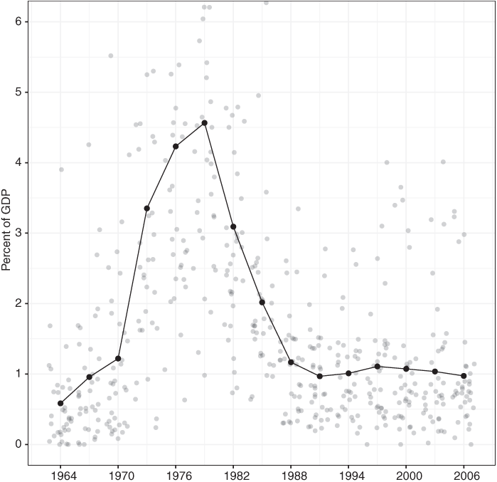
Figure 5.3 Federal aid to the thirty-four biggest US cities
Notes: Chart line connecting black dots represents annual average (not sum) transfer to group of thirty-four biggest cities.
Perhaps, however, we are looking for the representation of PBEIs in the wrong place. The parties are responsive, but not to the PBEIs of pivotal voters but to the PBEIs of their geographic bases. This is the second type of argument introduced earlier: parties are in conflict over PBEIs, based on the differing sectional interests of their core voters. We now turn to this second model.
Partisan Conflict and the Knowledge Economy
In Iversen and Soskice’s argument, governing parties face pressure to support the knowledge economy regardless of partisan hue. In arguments reviewed in this section, by contrast, competing parties represent differing spatially generated interests. This work dovetails with a large body of work on American politics that emphasizes the local economic roots of legislative representation (e.g., Becher et al. Reference Becher, Stegmueller and Kaeppner2018). Yet it goes beyond that focus by linking overall patterns of party competition to the shifting PBEIs emerging in the knowledge economy.
Rodden (Reference Rodden2019), for example, argues that the territorial basis of US representation has accentuated partisan conflict over PBEIs. Much attention has focused on Rodden’s analysis of the antimetro bias that accompanies single-member districts (a bias we discuss later in this chapter). Equally important, however, is his argument that the parties have realigned around the “odd bundles of policies [that] came together because of economic and political geography. The Democrats … have evolved into a diverse collection of urban interest groups, and the Republicans into an assemblage of exurban and rural interests” (Rodden Reference Rodden2019: 9).
Ansell and Gingrich (Reference Ansell, Gingrich, Hacker, Hertel-Fernandez, Pierson and Thelen2022) offer a complementary analysis focused on the nature of those “urban” and “exurban and rural” interests. Like Rodden, they argue that there is a strong tendency for the American political system to stovepipe PBEIs into national politics. In contrast to many European systems, the American system encourages spatially contiguous coalitions. Voters in PR systems do not need to form coalitions that can win local majorities, so they can support (smaller) parties that draw diffuse support from like-minded voters across the country. United States voter coalitions are instead territorially based and, according to Ansell and Gingrich, reflect the growing divide between the PBEIs of rising and declining locations.
Ansell and Gingrich are helpfully specific about what these PBEIs should be. They argue that Democrats, as part of a cross-class metro coalition, should become more favorable to policy bundles that include local redistribution (what they call “decommodification”) to hold their diverse coalition together. The same voters, however, should become less favorable to policies that allocate resources beyond metro areas (what they call “deconcentration”). Thus, even relatively affluent Democrats should embrace decommodification within metro blue America, but resist shifting resources toward nonmetro red America. In contrast, nonmetro voters – that is, Republicans – should favor such deconcentration, since it will reward their economically struggling territories. As we will discuss later, this last expectation is especially plausible given that incomes are higher in blue areas, so Democratic rather than Republican voters will finance the bulk of these benefits.Footnote 3
These are expectations about voter preferences, but like Iversen and Soskice and Rodden, Ansell and Gingrich suggest the parties will reshape their national party priorities in response. Indeed, a critical implication of all of these accounts is that both metro and nonmetro regions require policy supports from higher levels of governing authority. This is obviously true for non-metro areas that lack resources: left on their own, they are acutely vulnerable to ongoing decline. But it is also true for metropolitan areas. The urban knowledge economy’s local agglomerations require extensive public good provision (for transport, education, public safety, and social services) that is vulnerable to free riding. Addressing these challenges requires federal authority (Ogorzalek Reference Ogorzalek2018). For voters and parties on both sides, then, the challenges and opportunities reflected in PBEIs require an active response from leaders at higher levels of government.
Thus, we have clear expectations: the red coalition will shift toward supporting deconcentration (interregional redistribution); the blue coalition toward decommodification (intraregional redistribution). Here, too, these strong expectations confront striking paradoxes. In the remainder of this section, we briefly lay out these paradoxes. We then turn to the institutional, partisan, and policy filters that help explain them.
The Red PBEI Paradox
Red is increasingly the color of places the knowledge economy is passing by. Yet even as Republicans have become increasingly reliant on voters in nonmetro areas, national party elites have shown little inclination to transfer federal resources toward these constituencies. There are exceptions we will discuss, such as Republican support for fossil fuel extraction. The bottom line, however, is that deconcentration is almost nowhere to be seen within the GOP policy repertoire.
Instead, the signature party priority for at least three decades has been tax cuts for corporations and the rich – a goal that is unpopular even among Republican voters. These cuts have consistently offered their greatest benefits to big businesses and the super-wealthy, not rank-and-file GOP voters. Moreover, a large majority of these beneficiaries are located in blue metro areas rather than red nonmetro regions.
At the same time, Republicans have supported stark cuts in federal transfers to the states, which have fallen by roughly half since 1980 (see Figure 5.4). Given the progressive structure of federal taxes and spending, these transfers are highly favorable to nonmetro regions.Footnote 4 Republicans have also sought to cut social spending disproportionately received by voters in these regions. The most striking example is Medicaid, which GOP leaders have repeatedly sought to scale back – most recently, in early 2023, when they sought to tie Medicaid restrictions to a necessary extension of the so-called debt ceiling, a demand that threatened the first credit default in US history. In 2017, they came remarkably close to achieving even bigger cutbacks that would have been particularly devastating for nonmetro areas and red states (Levey Reference Levey2017).
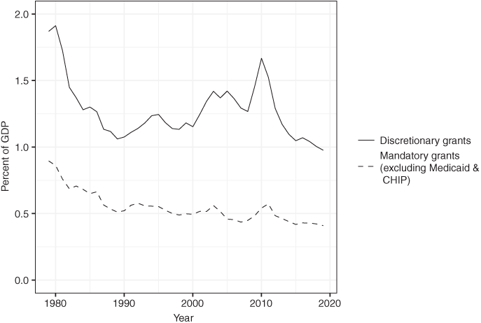
Figure 5.4 Federal grants for states and localities, 1980–2020
The Blue PBEI Paradox
Blue is the color of the knowledge economy in the United States. Given the increasingly tight link between population density, KE activity, and Democratic partisanship, we should expect Democratic elites to push for policies that support metro agglomerations. Meanwhile, they should embrace decommodifying policies (i.e., local redistribution) and reject deconcentrating ones. For the most part, however, these expectations have failed to pan out too.
Like the red PBEI paradox, the blue paradox has a positive and a negative side: unexpected policies that elites support and expected ones they do not. The key example of the former is interregional redistribution in favor of red America. As the fight over the ACA suggests, it is Democrats, not Republicans, who push for bigger transfers to nonmetro regions. Democratic elites have not simply backed existing fiscal policies that favor red nonmetro areas; they have pushed to increase this pro-red tilt, both by raising rates for top taxpayers (again, located mostly in blue America) and by expanding social policies that are particularly anemic in red America. If there is a party of deconcentration, it is the metro-oriented Democratic Party – precisely the opposite of what Ansell and Gingrich anticipate.
What about the other side of the ledger: PBEI-consistent policies that have failed to materialize? Here, what stands out is the relatively low priority placed by national Democrats on the challenges facing metro hubs that cannot be solved through local action alone. The key example is housing. Dynamic metro areas face a triple crisis of unaffordability, inadequacy, and inequality. Opinion polls suggest that the skyrocketing cost of housing is a huge concern of voters living in these regions, with strong support for various kinds of federal action (Demsas Reference Demsas2021; Hart Research Associates 2019). Housing supply shortages make productive urban centers much less productive (Hsieh and Moretti Reference Hsieh and Moretti2019), shut out millions of Americans who would benefit from proximity to knowledge hubs, and impose huge costs and risks on nonaffluent residents, including the growing specter of homelessness. These are exactly the sort of local inequalities that Ansell and Gingrich style decommodification could address.
To be sure, housing affordability is a problem of “superstar cities” worldwide. Yet the breadth of the US crisis and weakness of the US federal response stand out in cross-national perspective (Le Galès and Pierson Reference Le Galès and Pierson2019). It can be seen not only in the continuing failure of national Democrats to remedy local policy failures in this area – despite stepped-up efforts to do so in 2021, which we shall discuss later – but also in trends in federal housing outlays, which have declined dramatically from historic highs even as home prices and rental costs have moved sharply the other way (see Figure 5.5).
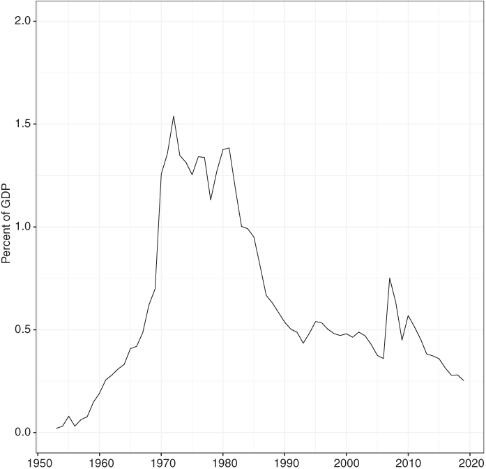
Figure 5.5 Federal housing and urban development spending
Table 5.1 summarizes the discussion thus far. The two types of arguments we have reviewed focus on different outcomes (overall policy outcomes vs. party stances). Yet they both foresee voters reorienting around the PBEIs that accompany the emergence of the KE. As the last column indicates, these expectations appear largely unmet.
The next section considers why. We first describe our concept of filters. We then show how these filters help account for the underrepresentation of PBEIs in the contemporary era.
Table 5.1 Representation of PBEIs in the US knowledge economy
| Focus of Account | Clearest PBEI(s) | Actual Outcomes |
|---|---|---|
| Iversen & Soskice – pivotal voter power in the KE | ||
| Overall policy | Pivotal voters support KE investments | Declining public investment in KE |
| Ansell & Gingrich/Rodden – partisan divergence in the KE | ||
| “Red” (Republican) Coalition’s Stance | “Deconcentration” (interregional redistribution) | Red PBEI Paradox: Resistance to deconcentration; tax cuts that are the opposite of deconcentration |
| “Blue” (Democratic) Coalition’s Stance | “Decommodification” (local redistribution), not deconcentration | Blue PBEI Paradox: Support for deconcentration; weak support for decommodification, esp. re. housing |
The Filtering of PBEIs
By filters, we mean institutional, partisan, and policy structures that refract, redirect, or block the expression of citizen interests as they move through the representative process. We divide our filters into three categories: political institutions, party coalitions, and policy regimes. Although students of representation appreciate the role of political institutions, the enormous power of this filter – especially in the United States – is not always appreciated. Less widely appreciated are the filters of party coalitions and policy regimes. Yet like formal institutions, these arrangements serve to organize some issues into national policymaking and organize others out.
Political Institutions as Filters
When thinking about representation solely in the US context, it is easy to take for granted the distinctive features of American political institutions or to treat them as historical constants. We shouldn’t, especially because the biases that these institutions produce have intensified and become more consequential. We focus on two biases in particular: the bias in favor of nonmetro interests (and the party that represents them) and the bias in favor of the status quo (and the party that seeks to preserve it). Each form of bias has grown in recent decades. Each also has enormous implications for the representation of PBEIs.
The underrepresentation of metro areas emerges out of several interlocking features of American institutions. Taken together, these impose what might be called a “density tax”: the denser a population, the less well represented it is. As the metro/nonmetro divide has widened, the density tax has not only increased; it has also become more aligned with partisanship.
The heaviest density tax, of course, applies in the Senate, the most malapportioned upper house in the rich world. The effects include, but are not limited to, giving the GOP a substantial seat edge (see Figure 5.6). In recent decades, Republicans have frequently enjoyed a Senate majority despite representing fewer people and receiving fewer votes in Senate elections.
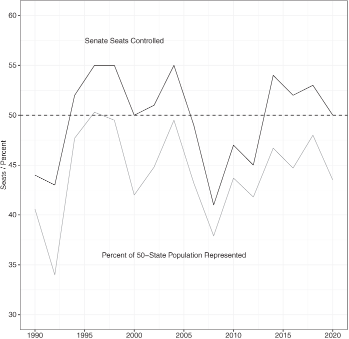
Figure 5.6 Republican overrepresentation in the US Senate
Antimetro bias is not limited to the Senate. As Rodden (Reference Rodden2019) argues, a system of single-member districts also imposes a density tax. Parties drawing their support from urban areas will be less efficient in translating votes into seats. As the parties have cleaved between metro and nonmetro areas, this tax has fallen on Democrats, awarding Republicans something like an extra dozen seats in the closely divided House (Powell, Clark, and Dube Reference Powell, Clark and Dube2020). Though there are signs the density tax has lessened as the suburbs of rich metros have become more blue, the penalty remains, and it is particularly pronounced in state legislatures. As Figure 5.7 shows, the average bias of statehouse maps toward Republicans has increased dramatically, driven by the density tax as well as the increasing frequency of GOP control over redistricting it helps produce.
Figure 5.7 Partisan skew in statehouse district maps, 1972 vs. 2020
The second crucial institutional filter is status quo bias. As students of comparative politics have long noted (Stepan and Linz Reference Stepan and Linz2011), no other affluent democracy places so many constitutional obstacles in the path of legislated policy change. In addition – and it is not a small addition – the Senate filibuster means that a supermajority of an already highly skewed institution is required to advance legislation.Footnote 5 Needing only forty-one votes, a minority that might represent less than 20 percent of the US population can block legislative action. In practice, narrow minorities block legislation, including very popular legislation, all the time.Footnote 6
Status quo bias is far from neutral. First, it empowers those who had power in the past. Existing policy can be seen as a kind of congealed influence, reflecting earlier power configurations (Moe Reference Moe2005; Pierson Reference Pierson, Fioretos, Faletti and Sheingate2016). Anything that makes these policies hard to change is likely to disadvantage those who were weakly represented in these earlier periods. This is particularly evident when it comes to racial and ethnic minorities, who are both concentrated in metro areas and now approach a majority of Democratic voters. For these voters – and the party seeking to represent them – the hurdle of American political institutions is often more like a wall.
Second, status quo bias empowers those who do not rely on national legislation to advance their interests. In general, this favors those who advocate minimalist government, or at least minimal regulation and redistribution – stances that often line up with the positions of the contemporary GOP. Like antimetro bias, the status quo bias of American institutions is favorable to one party over the other.
The interaction of these two biases draws our attention to the potential for “compounding bias,” when one institutional skew generates additional ones. As already noted, Republican state majorities, benefiting from the density tax, can gerrymander their own electoral maps, as well as those used to apportion seats in the US House. In another form of compounding bias, Republican Senators can exploit their chamber’s extreme skew to block Democratic judicial nominees, while racing their own to confirmation. The contemporary 6–3 conservative Supreme Court (which also reflects the antimetro bias of the Electoral College, which has elected two Republican presidents lacking popular vote majorities since 2000) is a vivid illustration of cumulative bias. The Court is also a far more powerful economic policymaker than often recognized, reinforcing the already-high barriers to an active response to both metro and nonmetro PBEIs. In each case, biases in one site create the capacity to enhance biases in others, even in a set of institutions expected to resist consolidations of partisan power (Pierson and Schickler Reference Pierson and Schickler2020).
We can sum up the discussion of institutional filters quickly. In the contemporary political environment, American political institutions operate in ways that greatly diminish the voice of metro interests in national policymaking, while also giving the Republican Party a representational edge that it can use to pursue its own aims or resist those of Democrats.
Party Coalitions as Filters
Party systems represent a second significant filter. Traditionally in American politics, it was assumed that national politicians would have an incentive to respond to strong place-based interests – that “all politics is local,” as Tip O’Neill famously put it. Yet as American politics has become more nationalized and polarized, local interests have faced a rockier path.
Two filtering effects are most important here. The first is the way polarization discourages elite efforts to serve local interests that are not aligned with party programs. American politics has always been based on two parties. But it has not always been based on two highly polarized and nationalized parties. In a context where two parties are not only dominant but polarized, they become powerful gatekeepers of national policymaking. Both voters and politicians are presented with increasingly binary choices, and the space to diverge from national priorities shrinks (Rodden Reference Rodden2019). Indeed, to the extent voters’ hardening allegiances are “affective” (driven by animus toward the other side), national party elites have much greater room to sidestep even deeply felt PBEIs, since voters are likely to stick with them even if they do.
At the same time that polarization decreases the scope for localized policy ventures, it increases the potential for priority setting by policy-demanding groups (Bawn et al. Reference Bawn, Cohen, Karol, Masket, Noel and Zaller2012). Groups that once might have floated between the parties now have incentives to side with one or the other, since their best opportunity for shaping policy is to enter into long-term coalitions with the party closest to them (Pierson and Schickler Reference Pierson and Schickler2020). In turn, party elites can use their increased running room with voters to serve these intense organized interests. In short, the power of resourceful party-allied groups relative to strong party identifiers is likely to increase.
It is important to emphasize that this filtering process may be quite functional for a party. Getting local issues expressed nationally may well create intraparty cleavages. Party leaders seek to institutionalize beneficial “trades” among intense allies, such as the Republican Party’s foundational trade of corporate-friendly tax cuts for conservative cultural stances. Because these deals are always vulnerable to destabilizing new issues, party leaders have strong incentives to keep such issues off the agenda. Traditionally, however, this has been difficult, which has repeatedly led to the breakdown of national issue-based coalitions (Schickler Reference Schickler2016). Parties struggled to keep divisive issues off the agenda because local politicians faced different incentives and constituencies than national ones. As this has become less true, the capacity of parties to keep disruptive local concerns off the table has grown.
We mention this last possibility because a central feature of the party filter today is that elite management of intraparty cleavages have tended to suppress, rather than foster, the representation of PBEIs. We have already mentioned the Republican Party’s prioritization of conservative pro-business policies. This has encouraged party elites to play on cultural grievances and white racial identity to mobilize voters, given that their economic priorities are largely inconsistent with nonmetro voters’ PBEIs. A very different but also very consequential intraparty cleavage has increasingly characterized the Democratic Party as it has come to rely on highly unequal metro regions. Affluent whites in these areas now largely back the Democratic Party, and as Ansell and Gingrich argue, they are relatively supportive of redistribution so long as it does not impose large costs on them. But they are much warier, we shall see, of policies that would threaten the privileges they enjoy because of local segregation and the resulting differential access to economic opportunities and public goods – a policy divide that cleaves the Democratic coalition along lines of both race and class. For Democratic party elites, this potential land mine encourages an emphasis on broader, if also less metro-beneficial, priorities.
Policy Regimes as Filters
Policy regimes represent our last and least-recognized filter. By policy regimes, we mean the inherited complex of rules and programs that determine the allocation of resources and authority in particular policy areas. While policies can, in theory, always be revised, they are highly path-dependent. Not only are those defending the status quo advantaged, but policies themselves make some changes easier to effect than others. Indeed, as the literature on “policy feedback” suggests, they shape whether certain changes are seen as possible or desirable at all, in part because they determine which allocations of valued resources are visible to voters and which are not.
Two features of the policy landscape are of particular relevance. The first is the degree to which policies automatically update to reflect changing circumstances. Revising entrenched policies is hard. Thus, default rules – whether, for example, policies expand to reflect the number of people eligible – matter enormously for how likely it is that they will continue to perform as expected, or “drift” away from their original purpose (Hacker, Pierson, and Thelen Reference Hacker, Pierson, Thelen, Mahoney and Thelen2015). This, we shall see, helps explain the anemic US response to the shifting contours of the KE.
The second crucial feature is the extreme decentralization of US policymaking, especially in core areas of policy that affect the knowledge economy, such as housing, land use, education, infrastructure, and policing. This extreme decentralization coexists with weak measures to even out the administrative and budget capacities of differing localities, such as fiscal equalization and revenue sharing. In cross-national perspective, American policymaking is not merely decentralized; it is decentralized in ways that accentuate inequalities across jurisdictions.
Little in these arrangements is constitutionally required. Unmentioned in the nation’s founding charter, localities are creatures of the states. Instead, these arrangements are constituted by longstanding policies that reflect the mutually reinforcing effects of path dependence and the distribution of power (Trounstine Reference Trounstine2018; Weir et al. Reference Weir, Wolman and Swanstrom2005). The resulting regime divides authority between localities and higher levels of government in ways that are both relatively invisible and pose high hurdles to positive-sum collective action.
Most notably, property-tax financing of local public goods and highly decentralized authority over land use – along with the ability of suburban communities to evade the tax and regulatory reach of cities – reinforce the influence of affluent white homeowners and give them strong incentives and ability to oppose policies that would allow less-affluent outsiders access to hoarded public goods or housing. Simultaneously, this regime makes it very hard to push these issues up to higher policy levels, where these forces of resistance would be less advantaged.
We can see how these three sets of filters play out by revisiting our two paradoxes. In the next two sections, we look again at the paradoxical positions of the Democratic and Republican Parties, showing how key filters help explain the weak (and sometimes upside-down) relationship between the stances of the parties and the PBEIs of red and blue America.
The Red PBEI Paradox Revisited
Republicans have pursued policies that offer little or nothing to their geographic bastions or even hurt these areas. Meanwhile, they have failed to pursue policies that might transfer resources toward declining red regions. The filters – particularly the institutional antimetro and status quo biases and the nature of the GOP coalition – help us understand these puzzling patterns.
The Institutional Filter
The role of the institutional filter is hard to overstate. First, as noted, it helps explain why Republicans have dominated legislatures in many states that would be closely divided, or controlled by Democrats, absent the density tax and aggressive gerrymandering. Second, at the national level, it has given Republicans a stronger hand than their popular vote totals or support for their agenda would suggest. The Senate filibuster has proved especially useful for Republicans, allowing the party to tie up governance in ways that are very hard for voters to understand or punish. In particular, it has short-circuited the kind of cross-party coalitional efforts that often undergirded sectional policy in the past.
Although our focus is on national representation, we should stress that these institutional biases also play out at the state level. In another chapter written by two of us with Grumbach (Grumbach, Hacker, and Pierson Reference Grumbach, Hacker, Pierson, Jacob, Hertel-Fernandez, Pierson and Thelen2022), we argue that GOP leaders have generally pursued policies ill-suited to a globalized knowledge economy. Indeed, we find that, controlling for prior education levels and manufacturing strength, red states that have pursued the most conservative economic policies have the lowest workforce participation, wages, and median incomes. One reason why red-state Republicans have managed to pursue such policies and still retain strong majorities is that the antimetro bias is at least as strong at the state level as at the national level.
The Party Coalition Filter
While the institutional filter is helpful in understanding Republicans’ outsized governing influence – and, in particular, their ability to block even popular policies – it is less helpful for explaining what they do with their influence. Here the party filter – the peculiar shape of the GOP’s party coalition – becomes much more important.
In brief, the Republican Party has become a national coalition uniting two sets of groups: “plutocratic” organizations, such as business lobbies and billionaire donors, that shape the party’s economic policies; and “right-wing populist” organizations, such as conservative religious groups and the National Rifle Association, that shape the party’s electoral strategies and social issue priorities. Stretching the definition of groups, the latter organizations also encompass right-wing media (which has no real counterpart on the left). The stability of this “plutocratic populist” coalition has rested in part on the willingness of leaders on the populist side – notably, those allied with the Christian right – to jettison demands for economic policies that would have benefited their mass base but were opposed by the party’s plutocratic allies (Hacker and Pierson Reference Hacker and Pierson2020).
Whenever and wherever such conflicts have arisen, the PBEIs of red America have given way to the priorities of rich America. We have already mentioned high-end tax cuts, the cornerstone of GOP economic policy. Given the spatial distribution of affluence in the United States, the direct beneficiaries of these tax cuts disproportionately reside in blue states (or abroad). Moreover, these cuts not only bypass most Republican voters. They also pose a clear fiscal threat to the GOP electorate over the long term, generating acute pressures on major social programs on which aging red-state voters disproportionately rely, including Social Security, Medicare, and Disability Insurance. In short, tax cuts not only disproportionately go to blue America; they restrict the fiscal space for “deconcentrating” initiatives that could help red America.
As noted, a version of this dynamic has already played out on healthcare. GOP “repeal and replace” plans for the Affordable Care Act (ACA) would have had a devastating impact on nonmetro America. Yet almost all national Republicans supported them. They did so in part because repealing the ACA would have allowed a rollback of the high-end taxes that provided the program’s progressive financing. Moreover, the associated Medicaid cuts could be leveraged into even deeper tax cuts in the future. Only the defection of a handful of Senate Republicans saved the ACA.
The rise of Donald Trump did not much change this dynamic. While doubling down on right-wing populism, Trump embraced both massively skewed tax cuts and the ill-fated ACA repeal. He talked about but did little to press for adequate federal spending to deal with the opioid epidemic – a core dimension of the “deaths of despair” disproportionately ravaging areas of GOP strength (Case and Deaton Reference Case and Deaton2020). Nor did he follow up on repeated promises of infrastructure or prescription drug proposals that might have helped nonmetro voters.Footnote 7
Indeed, even the one clear area of PBEI-party affinity suggests the importance of coalitional considerations. National Republicans have taken increasingly aggressive stances with respect to energy deregulation, the use of federal lands, and resistance to action on climate change. These stances have certainly helped a handful of red states (in particular Alaska, North Dakota, and Wyoming), but they have proved even more lucrative for the fossil fuel industry. Indeed, given the extreme geographic concentration of energy production in a few red states, these stances are better seen as successful rent-seeking by corporate backers of the GOP than as a viable growth strategy for red America.
Are Voters, Not Filters, the Source of the Paradox?
Before we move to the Democratic side of the story, we want to address an objection that analyses of the Republican Party like ours invariably provoke: the disconnect is not between GOP voters and their representatives; it is between GOP voters’ economic interests and how they vote. As noted, however, we do not think the explanation for the patterns we find is that GOP voters are committed to policy positions at odds with the shifting PBEIs of red America.
To be sure, voters operate in a complex environment in which party elites and allied groups provide powerful cues and no small measure of misinformation. Most people have limited understanding of policy, and partisanship and social identities heavily color what they think they know. For example, Republicans are much more likely to associate government spending with Black Americans, immigrants, and means-tested benefits (Krimmel and Radar 2021). Growing negative affect toward the other party further limits the scope for policy issues to matter in electoral politics. To this list of complications, we should add the ability of party elites to use second-dimension issues – particularly those concerning religious and racial identities – to reduce the salience of voters’ economic stances (Hacker and Pierson Reference Hacker and Pierson2020). Given the relatively homogenous racial and religious identities of GOP voters, a significant share can be motivated primarily by the cultural, racial, ethnic, and regional resentments that party elites have stoked. Indeed, a core reason we focus on PBEIs is that we want to avoid treating answers to survey questions – which necessarily incorporate these factors – as synonymous with preferences, much less interests.
Nonetheless, there is substantial evidence that Republican voters are not driving GOP economic policy and, indeed, that many of the party’s PBEI-inconsistent stances are unpopular among its own voters. For at least two decades, elite Republicans have made the combination of high-end tax cuts and sharp spending cuts the centerpiece of their fiscal plans. This was the formula embodied, for example, in Paul Ryan’s high-profile budget blueprints of the early 2010s. According to national polling, the Ryan plan lacked majority support not only among Democrats but also Republicans – and, indeed, even among GOP donors. Only among donors with annual incomes greater than $250,000 did support outweigh opposition (Hacker and Pierson Reference Hacker and Pierson2020).
More recently, the failed effort to repeal the ACA and successful effort to pass highly skewed tax cuts in 2017 were both overwhelmingly unpopular, failing to command strong support even from Republican voters. Indeed, they were the two least popular major federal initiatives considered and/or passed between 1990 and 2017 (Hacker and Pierson Reference Hacker and Pierson2020).
Perhaps most revealing, however, are state-level ballot questions. Six of the eleven red states where ballot initiatives are allowed have held votes on Medicaid expansion – a policy universally opposed by national Republican elites, as well as most state GOP leaders. Every one of these states voted in favor of Medicaid expansion. Similarly, Republican elites have strongly resisted increases in the minimum wage. Since 2006, however, eleven red states have held ballot questions to raise the state minimum. All eleven passed by very large margins.
These results suggest that red state legislatures are blocking popular initiatives, and the behavior of these legislatures only reinforces this conclusion. In Michigan, Republicans enacted their own legislation to preempt an initiative – and then promptly repealed it once the election was safely past. In Idaho, the Republican legislature responded to a successful initiative expanding Medicaid by radically restricting the initiative procedure. Missouri may well follow suit. In other red states, legislatures have ignored proposals to expand the minimum wage, among other popular initiatives.
In sum, the disconnect between the PBEIs of red America and the policy agenda of the Republican Party does not seem to be voter-driven. Instead, it bears the imprint of both America’s distinctive institutions and the particular character of the GOP coalition. Together, these simultaneously motivate nonresponsive party stances (party filter), undercut accountability (institutional filter), and increase the governing strength of the Republican Party relative to its popularity (institutional filter). The result is a nationalized interest group coalition that places top priority on business- and affluent-friendly policies regardless of their sectional impact.Footnote 8
The Blue PBEI Paradox Revisited
What we have called the blue PBEI paradox constitutes at least three puzzles. First, Democrats have not strengthened – or even sustained – KE investments. In part, this is simply a reflection of the Republican Party’s institutional edge. Nonetheless, we do not think GOP blocking can fully explain the notable fall in public investment discussed earlier.
The second and third puzzles squarely concern party stances, rather than policy outcomes: Why have national Democrats proved so eager to embrace deconcentrating policies that distribute outsized benefits to red America? And why have they proved so reluctant to address the collective action challenges of metro areas, particularly with regard to housing?
Not surprisingly, the institutional filter again looms large. However, both the character of the Democratic coalition and of the US policy regime play an important role as well.
The Institutional Filter
Both the antimetro and status quo biases of American political institutions weaken the capacity of national Democrats to update economic policies to reflect the changing needs of the knowledge economy. They do so, moreover, in ways that reflect specific features of the US policy regime we will discuss shortly. For now, the key point is that all the advantages enjoyed by the party that represents nonmetro regions and seeks to block government action are disadvantages for the party that represents metro regions and seeks to expand government action.
Moreover, these disadvantages have been growing. Urban America once enjoyed relatively strong representation in American national politics (Ogorzalek Reference Ogorzalek2018). But the density tax has been rising. Even as blue metros have gained more and more economic ground – Joe Biden won counties that produced 70 percent of US GDP in 2020 (Muro et al. Reference Muro, Byerly-Duke, You and Maxim2020) – they have lost more and more political ground. The biases of Senate apportionment, House, and state districts naturally favoring nonmetro areas, and aggressive gerrymandering and other measures (often sanctioned by stacked courts) compound to tilt the playing field farther and farther.
The eroding political clout of metro interests is not simply a reflection of the institutional filter. Urban representatives have never been a majority in the national legislature. They relied for their power on a capacity to form party coalitions with representatives from nonmetro districts. Today’s weakness of metro America also reflects profound changes in the party system.
The Party Coalition Filter
Cities have not always been solidly blue. Since the New Deal, however, their political fortunes have been tied to the national Democratic Party. During the New Deal Era, the power of the nation’s major urban centers rested on their ability to form logrolling agreements with Southern representatives, facilitated by shared partisanship (Ogorzalek Reference Ogorzalek2018). This arrangement unraveled after 1975 as the South (and eventually nonmetro districts outside it) realigned to join the Republican Party. Indeed, the earliest policy impact of this realignment was the collapse of the coalition that had supported major national urban initiatives in the 1960s and 1970s (Caraley Reference Caraley1992). Conservative Democrats (mostly from Southern and/or nonmetro places) joined the “Reagan revolution” and gutted these programs – in retrospect, an intermediate step as those electoral jurisdictions transitioned into Republican hands.
Trends since the early 1980s have further diminished the voice of cities in national policymaking. As Ogorzalek (Reference Ogorzalek2018) has argued, the Southern Democratic retreat from its New Deal alliance with cities, the growth of the suburbs, and the decline of urban political machines all weakened the strong place of cities within the party’s organized coalition. The problem is not merely that cities now have a weaker hold on the Democratic Party than they once did. Republican politicians who represent urban areas have all but vanished, and with them, the incentives to fashion cross-party compromises in support of metro PBEIs.
The character of the Democratic coalition can also help explain why Democrats in power have pursued an agenda heavy on deconcentration. To some extent, the antimetro bias of American institutions can help to explain this: due to the density tax, Democrats must reach beyond their core metro supporters to win elections. Yet it is hard to see how the institutional filter can explain why Democratic priorities envision redistributing so many resources to deeply red regions of the country where the party has no real chance of success. Nor do Democratic voters appear to be the main catalysts here. Most are probably unaware that the policies their elected officials advance entail such substantial spatial redistribution (though, unlike the case of the red state paradox, there is little sign that they would actively oppose such initiatives).
The subject requires far more research, but we would stress the role of party coalitions here, too – specifically, the role of intense policy demanders within the Democratic coalition. These include labor unions, civil rights organizations, progressive economic groups, and a variety of allied social movements. As is true on the Republican side, these organized elements of the coalition are increasingly national in their focus, increasingly working with “their” party alone, and increasingly at odds with the other party’s social and economic policies. And as is also true on the Republican side, these organized actors mostly “float above” local and regional differences: their funding comes from nationally oriented donors and foundations, their leadership and headquarters are generally based in DC, and their activities – even if sometimes focused below the national level – are rooted in their increasingly tight alliances with an increasingly nationalized party. Indeed, the Democratic Party arguably lacks some of the localized connections that have animated GOP politics in recent years (mostly on the cultural side of the Republican agenda). With the partial exception of organized labor, Democrats lack the widespread community infrastructure embodied in the Christian Right, nor have Democratic-aligned groups and movements proved as adept at using American federalism to advance their goals on a state-by-state basis (Hertel-Fernandez Reference Hertel-Fernandez2019).
The vision of party-aligned groups on the left is not just national in focus but also universal in aspiration. By this we mean they tend to advance goals – from greater ability to form a union to improved access to affordable healthcare to sustained reductions in poverty – that aim to provide greater support for low- and middle-income Americans, whatever their backgrounds and wherever they live. This vision of a universal policy floor is what you might expect from nationally focused groups with stated commitments to equality, especially the party’s mass-membership backbone: organized labor. Yet there is also a strategic rationale that seems important to many of their leaders: that the party’s multiracial coalition is best held together through appeals and proposals that center shared economic interests, rather than those specific to place, race, or other salient divides.Footnote 9 In another recent analysis (Hacker et al. Reference Hacker, Malpas, Pierson and Zacher2023), for instance, we find that both Democratic Party platforms and the tweets of recent Democratic presidents and members of Congress have overwhelmingly emphasized economic issues and universal economic policies (in contrast with Republican leaders, who emphasize cultural appeals on Twitter).
For these policy demanders, then, Ansell and Gingrich’s decommodification – downward redistribution within richer areas – is not enough. They want a generous policy floor nationwide. Given America’s highly uneven and decentralized fiscal federalism, that floor can be created only by strengthening federal redistribution in ways that offer disproportionate benefits to declining areas where supports are weak. In other words, national redistribution of the sort advocated by groups aligned with the Democratic Party tends to produce substantial deconcentration, and this deconcentration in turn tends to benefit states aligned with the Republican Party. By way of illustration, only one of the ten states with the highest ratio of federal benefits to federal taxes – that is, whose residents get back more from the federal government than they pay to it – has consistently voted for the Democratic presidential candidate since 2000 (Hawaii), while nine of the ten with the lowest ratio of federal taxes to benefits have consistently voted for the Republican candidate.Footnote 10
The Policy Filter
Many of the problems facing metro America boil down to one: cities lack the tools or authority to deal with collective action challenges they face. The erosion of federal funding for key investments in metro economies has deprived these areas of vital resources on which they once relied to manage the exigencies of urban interdependence. Of course, the institutional biases already discussed are major causes of this trend. But the structure of public policy is also implicated. As noted, different programs are more or less vulnerable to erosion over time depending on whether they require periodic legislative updating. While some federal spending programs are “mandatory” – meaning their benefits cover everyone eligible and expenditures rise automatically in response to demand – many are “discretionary” and must be reauthorized regularly. Most of the major spending programs of importance for the knowledge economy fall into the discretionary category, including support for science, education, housing, and mass transit. To grasp the full effect of the institutional filter, then, requires looking at the way existing policies privilege some kinds of policy updates while discouraging others.
The policy filter is even more clearly implicated in the final PBEI puzzle – the failure of the Democratic Party to respond adequately to the collective action challenges facing metro America, particularly with regard to housing. There is a broad consensus among economists that land use and zoning rules are the principal causes of the housing crisis. These are not national or even state policies; they are local policies, with each of the nation’s tens of thousands of local governments controlling development within its borders. This fragmented system allows suburbs to free ride on cities, magnifies the influence of affluent white homeowners (Einstein et al. Reference Einstein, Glick and Palmer2020), and empowers “home-voters” who are most likely to show up in low-visibility local elections and have extreme and intense preferences on this dimension (Marble and Nall Reference Marble and Nall2020). The result is widespread use of exclusionary zoning, inadequate affordable housing, and stark racial and economic segregation within and across jurisdictions (Trounstine Reference Trounstine2018). Much of the burden falls on those denied access to high-productivity places. But it also imposes huge costs on the most disadvantaged residents of metro America, disproportionately non-white, as well as the economy overall.
Here again, voter preferences do not seem to be the decisive factor. There is strong support for measures to provide more affordable housing (Demsas Reference Demsas2021; Hart Research Associates 2019). The problem is unfavorable political dynamics at the local level, rooted in a highly decentralized and entrenched policy regime, in which intense minority interests are privileged at the expense of broader majority interests. The result is a set of increasingly dire problems that affect millions of Democratic voters and cry out for national leadership.
Yet Democratic elites at the national level have largely failed to respond to these critical needs. To do so would require challenging localized policymaking, and that has proved something that party leaders have shown limited ability or inclination to do. The entrenchment of localized control makes the task hard to begin with. On top of that, it also creates a huge potential wedge within the Democratic coalition between affluent, white, home-owning voters and less-affluent portions of the party’s metro-based electorate. For Democrats, there are good reasons to organize this issue out of their agenda, or at least to focus on symbolic or half-hearted measures that do not threaten to activate intense potential cleavages within the party’s electorate.
In short, the institutional, party, and policy filters all help explain the underrepresentation of the PBEIs of blue metro areas, even as the knowledge economy has made their policy interests and party allegiances increasingly distinct.
Conclusion
The rise of the knowledge economy has produced a growing economic fissure between metro and nonmetro America, and this fissure has mapped closely onto the polarized divide between the Republican and Democratic parties. In a territorially organized polity, these changes might be expected to create pressures for elected officials to shift their priorities to reflect the evolving place-based interests of their constituents – a recurrent historical pattern in American politics that prominent scholars have argued is happening again today.
Despite these pressures, however, we find more refraction than reflection. There is limited sign of Iversen and Soskice’s predicted realignment of partisan competition around promotion of the knowledge economy. Indeed, the last two decades have witnessed a marked decline in policy support for the knowledge economy – a potentially fateful development.
Nor have the parties reoriented themselves toward the PBEIs of their geographic bastions as might be expected. Despite increasing reliance on nonmetro voters, the Republican Party has done little to support Ansell and Gingrich’s “deconcentration,” focusing its priorities on the demands of wealthy voters and corporate interests rather than those of its broad voting base. Instead, if there is a party backing deconcentration, it is the Democrats – driven in part by their own organized allies, who emphasize the need to raise the social policy floor in nonmetro regions. At the same time, even as the Democratic Party has come to dominate the nation’s metro agglomerations, national Democrats have failed to robustly address the hugely costly dilemmas associated with local control that threaten these blue locales’ continuing success.
To explain these paradoxes, we have argued for a greater focus on what we call “filters” – durable features of a polity that mediate the influence of citizens on governance. In asking whether PBEIs make this transit, we seek to avoid the assumption common in the prevailing filter-free view of representation that all issues of fundamental concern will become manifest in policymaking. Because of the institutional, party, and policy filters, there is no guarantee that voters will see a clear link between their electoral choices and their PBEIs, or that politicians will respond to those PBEIs even if voters articulate them. In particular, there is no guarantee that local economic interests will be stovepiped up to higher levels of government where effective action can be taken.
Our filtered approach to representation emphasizes three refracting features of contemporary American politics. First, geographic partisan polarization has accentuated longstanding biases in US political institutions that impose a density tax on voters in metro areas and privilege the policy status quo. This, in turn, has made ongoing policy adaptation to the knowledge economy difficult and shifted the partisan balance of power toward the Republican Party. Second, in an increasingly nationalized and polarized party system, the character of party coalitions is another powerful filter of local economic interests. Organized groups operating on a national scale have strong incentives to pick sides, orient their activities around national party agendas, and take advantage of parties’ increased agenda-setting power. Especially with affective partisan identities increasingly driving voter behavior – identities that map onto and have roots in racial and ethnic conflict as well as growing geographic inequality itself – party elites may well feel empowered to pursue policies with support from organized allies even when those policies are at odds with voters’ local concerns.
Finally, the distinctive structure of the US public policies weighs heavily on the representation of metro interests today. Localized control over zoning and other vital policy levers places a formidable barrier in the way of national action to support the knowledge economy and help urban agglomerations overcome collective action problems. The party filter also matters here, too, for unsettling these costly arrangements could also unsettle the Democratic Party’s alliance between the privileged and the disadvantaged and between urban and suburban residents of metro America. Thus, Democrats too face distributional tensions between the most affluent portions of their coalition and their broader voting base.
Whether those tensions can be resolved depends in part on the heated battles taking place in Washington as we write. In 2021–2022, the razor-thin Democratic majority in Congress failed to enact an ambitious package of domestic social policies. However, it did pass three bills (two with modest Republican support, one enacted on a party-line vote) that began to address the huge backlog of urban infrastructure needs and the long-term stagnation of investment in advanced R&D. It is important to recognize, though, that these new initiatives were paired with a great deal of investment in nonmetro areas, in part because the pivotal Democrat in the Senate was Joe Manchin of (rural) West Virginia. Notably, the investments envisioned so far include substantial funding for infrastructure and clean energy in red areas of the country. For example, nearly four-fifths of the clean energy investments announced by May 2023 under the 2022 Inflation Reduction Act are set to take place in Republican House districts. Meanwhile, the new House Republican majority has voted to repeal these incentives (a symbolic step, given Democratic control of the Senate, but one that could get caught up in the aforementioned debt ceiling fight). As the veteran journalist Ronald Brownstein aptly notes, “This opposition contravenes the traditional assumption that politicians almost always support the economic interests creating opportunity for their constituents.”Footnote 11
We do not think the filters we have examined completely explain this striking disconnect, much less all the patterns of representation we see. A focus on the institutional, party, and policy filters does not fully capture the role of race, for example – though distinctive elements of that role do come into view, as we hope we have shown. Nonetheless, the filters play a fundamental role in explaining why PBEIs occupy such a limited and often paradoxical place in American politics today. National party priorities cannot be simply “read off” of voters’ preferences – we need to see how they are refracted through the filters. Because of the nationalization and polarization of the parties within a distinctive electoral system, neither Democrats nor Republicans are likely to be penalized if they neglect PBEIs as they would have in the past.
To be sure, there is scope for PBEIs to come to play a larger role, and party coalitions can and do change over time. A crucial question is whether the investments being made today might bolster Democrats’ standing outside their metropolitan base, in turn pressuring Republicans to be more responsive to the PBEIs of their constituents. Another is whether organized elements of the business community that benefit from such investments might become more willing to actively back the Democratic Party and even perhaps push it to focus more on metro investments. Ultimately, the question is whether the filters will continue to dampen the incentive for US representative institutions to produce active federal policies responding to the dramatic shift in the geography of prosperity that the transition to the knowledge economy has fostered.
This is not a question for American policymakers alone. All advanced democratic societies are grappling with it in one way or another. Many of the features of the American political landscape that we highlight are unusual. Those features may well help to account for the growing cross-national evidence that the United States is a significant outlier with regard to the representation of citizen preferences in an increasingly unequal economy. Yet we believe a filtered approach to representation has relevance beyond the American case. Our hope is that this paper can contribute to the ongoing effort to consider how countries’ institutions, party systems, and policy inheritances influence the degree to which the concerns of ordinary citizens are translated into public policy.


 Open access