Negative Exponential Demand

As the first alternative to demand elasticity being determined by membership of a risk-group and invariant to changes in the premium (that is, iso-elastic), suppose that demand elasticity is an increasing function of the premium π, and the same irrespective of the individual’s risk-group. One example of this is represented in Figure A.1. The linear relationship shown between demand elasticity and premium is assumed to apply identically for both high and low risk-groups.

Figure A.1 Demand elasticity linear in premium (leads to negative exponential demand)

In Figure A.1, the values of 0.2 and 0.8 marked by the two circles are the demand elasticities corresponding to premiums of 0.01 and 0.04, respectively. Assuming the true risks are 0.01 and 0.04 as in Chapter 5, these values of 0.2 and 0.8 represent the fair-premium demand elasticities for low and high risks, respectively.

The particular linear relationship in Figure A.1, where the straight line representing demand elasticity passes through the origin, amounts to saying that the fair-premium demand elasticities λ_i vary in proportion to the corresponding fair premiums μ_i (for risk-groups i = 1, 2), that is:

(A.1) $\frac{{\lambda }_2}{{\lambda }_1}=\frac{{\mu }_2}{{\mu }_1}$

A suitable model for demand elasticity ɛ(π) is then:

(A.2) $\epsilon (\pi )=\frac{{\lambda }_1}{{\mu }_1}\pi =\frac{{\lambda }_2}{{\mu }_2}\pi$

Recalling that demand elasticity can be written as the log–log derivative:

(A.3) $\epsilon (\pi )=-\frac{\partial \log \left[d({\mu }_i,\pi )\right]}{\partial \log \pi }$

We can then equate Equations (A.2) and (A.3) and solve to obtain the negative exponential demand function:

(A.4) $d({\mu }_i,\pi )={\tau }_i\exp \{\left(1-\frac{\pi }{{\mu }_i}\right){\lambda }_i\}$

where

• τ_i = d(μ_i, μ_i) is the ‘fair-premium demand’ for population i, that is the proportion of risk-group i who buy insurance at an actuarially fair premium, that is when π = μ_i

• μ_i is the risk (probability of loss) for members of risk-group i

• λ_i is the fair-premium demand elasticity for members of risk-group i, that is the demand elasticity when an actuarially fair premium π = μ_i is charged.

This demand function satisfies the axioms for a demand function which were stated in Chapter 5.

Negative exponential demand has the characteristic property that the second derivative is the first derivative squared, divided by the original function.

Generalised Negative Exponential Demand

Now suppose that instead of the linear function shown in Figure A.1, demand elasticity is an increasing but nonlinear function of the premium, and the same irrespective of the individual’s risk-group. Two cases are shown in Figure A.2. For a continuous demand function, demand elasticity must go to zero when the premium goes to zero; so a straight line between the two points representing high and low risks’ fair-premium demand elasticities in these plots would not give a sensible model. Instead, we need to fit a nonlinear curve which passes through the two points and the origin. Suitable nonlinear curves can be fitted such that:

(A.5) $\epsilon (\pi )={\lambda }_1{\left(\frac{\pi }{{\mu }_1}\right)}^{\mathit{n}}={\lambda }_2{\left(\frac{\pi }{{\mu }_2}\right)}^{\mathit{n}},\text{for some}n$

Observing that $\epsilon ({\mu }_1)={\lambda }_1$ and $\epsilon ({\mu }_2)={\lambda }_2$, where the λ_i are defined as the fair-premium demand elasticities as earlier, we can find n as:

(A.6) $n=\frac{\log ({\lambda }_2/{\lambda }_1)}{\log ({\mu }_2/{\mu }_1)}$

The parameter n can be interpreted as the ‘elasticity of elasticity’, also known as the ‘second-order elasticity’.

In this specification, demand elasticity as a function of premium is: for n = 1, linear (as in the previous example, Figure A.1); for 0 < n < 1, concave (as in the left-hand panel of Figure A.2); and for n > 1, convex (as in the right-hand panel of Figure A.2).

Equating Equation (A.5) to the definition of demand elasticity in Equation (A.3) and solving, we obtain the generalised negative exponential demand function:

(A.7) $d({\mu }_i,\pi )={\tau }_i\exp \{\left[1-{\left(\frac{{\pi }_{}}{{\mu }_i}\right)}^{\mathit{n}}\right]\frac{{\lambda }_i}{n}\}$

Figure A.2 Demand elasticity curvilinear in premium (leads to generalised negative exponential demand)

Note that the demand functions discussed earlier are both special cases of this generalised negative exponential demand function: n = 1 corresponds to negative exponential demand, and n → 0 corresponds to iso-elastic demand.

Exponential Power Demand

The exponential power demand function corresponds to the generalised negative exponential demand formula, but with n = λ_i. It is a very flexible, but rather intractable, formulation which allows a wide range of levels and curvatures for the demand curve to be specified. Exponential power demand is specified as follows:

(A.8) $d({\mu }_i,\pi )={\tau }_i\exp \left\{1-{\left(\frac{\pi }{{\mu }_i}\right)}^{{\lambda }_i}\right\}$

This specification was suggested in De Jong and Ferris (Reference De Jong and Ferris2006), and I adopted it in my early papers on loss coverage (Thomas, Reference Thomas2008, Reference Thomas2009). With hindsight it would have been better to use a more tractable specification, such as iso-elastic demand.

Table A.1 summarises the functional form and demand elasticity for each of the four demand functions discussed above. In the right-hand column of Table A.1, the specification of demand elasticity as a function of λ_i becomes increasingly sophisticated as one moves down the page.

Table A.1 Functional form and demand elasticity for common demand functions

Demand model	Functional form of $d({\mu }_i,\pi )$ (multiplier ${\tau }_i{p}_i$ omitted in each case)	Corresponding demand elasticity
Iso-elastic	${\left(\frac{\pi }{{\mu }_i}\right)}^{-{\lambda }_i}$	${\lambda }_i$
Negative exponential	$\exp \left\{\left(1-\frac{\pi }{{\mu }_i}\right){\lambda }_i\right\}$	$\frac{{\lambda }_i}{{\mu }_i}\pi$
Generalised negative exponential	$\exp \{\left[1-{\left(\frac{{\pi }_{}}{{\mu }_i}\right)}^n\right]\frac{{\lambda }_i}{n}\}$	${\lambda }_i{\left(\frac{\pi }{{\mu }_i}\right)}^{\mathit{n}}$
Exponential power	$\exp \left\{{1-\left(\frac{\pi }{{\mu }_i}\right)}^{{\lambda }_i}\right\}$	${\lambda }_i{\left(\frac{\pi }{{\mu }_i}\right)}^{{\lambda }_i}$

The differences between the four demand functions can also be understood graphically. Figure A.3 plots the four demand functions for a single risk-group with μ = 0.01 and the specimen parameter values λ = 0.5 (the top curve in each panel), λ = 1.0, and λ = 1.5 (the bottom curve in each panel). It can be seen that the lower right panel showing exponential power demand has the most flexible specification: as the λ-parameter is changed from 0.5 to 1 to 1.5, the demand curve ‘sweeps’ across a wide area, and exhibits a large change in curvature. The first three panels in Figure A.3 – iso-elastic, negative exponential and generalised negative exponential demand – are all particular cases of generalised negative exponential demand (for n → 0, n = 1 and n = 2, respectively). It can be seen that as n increases from panel (1) to panel (3), demand decreases at all premium levels.

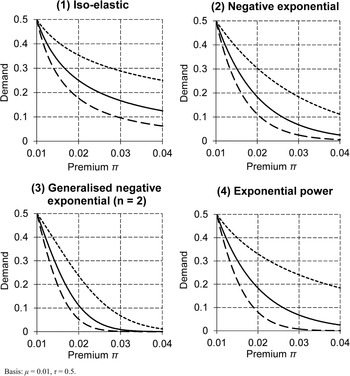
Figure A.3 Plots of four demand functions for a single risk-group for λ = 0.5 (top line), λ = 1.0 (middle line) and λ = 1.5 (bottom line)

Unlike the other demand functions in this chapter, exponential power demand is not predicated on demand elasticity being the same function of premium irrespective of risk-group (as shown in Figures A.1 and A.2). Therefore loss coverage under this demand function cannot be plotted against a single demand elasticity at the equilibrium premium, as was done for other demand functions shown in Figure 5.8). However, using a slightly different interpretation of ‘demand elasticity at the equilibrium premium’, we can obtain a similar inverted-U shaped graph, showing that loss coverage is maximised by intermediate demand elasticity. The details are given in Thomas (Reference Thomas2009).

How Multiple Roots Can Arise

Graphically, a root of the profit equation is determined where the expected profit crosses the x-axis. Figure B.1 illustrates this for the typical parameters (μ₁, μ₂) = (0.01, 0.04), α₁ = 0.9 and λ₁ = λ₂ = 1. Note that as the actual premium increases above the equilibrium level, insurers make progressively increasing profits; and as the premium decreases, insurers make progressively increasing losses. The monotonic nature of the profit function implies that the equilibrium shown is stable and well-defined. Under deviations from equilibrium, profit is negative when equilibrium requires an increase in premium and vice versa (that is, the profit ‘signal’ always has the ‘right sign’).

Figure B.1 Profit function for (λ₁, λ₂) = (1, 1): single root

Now suppose we change the parameters to α₁ = 0.992, λ₁ = 5 and λ₂ = 1. Note that these values are extreme, in particular the high risk-group is extremely small, and there is a very large difference in demand elasticities between risk-groups. The result is shown in Figure B.2. In the left panel, the y-axis has the same scale as in Figure B.1. In the right panel, the y-axis has a 10× zoom.

In the left panel, notice that profit is nearly zero over the full range of potential premiums (that is, a ‘wrong’ premium leads to only a weak profit ‘signal’). In the zoomed right panel, note that the profit function has three roots, representing three potential equilibria. At the ‘middle’ root, small increases in premium above this level initially lead to increasing losses for insurers and vice versa (that is, the profit signal has the ‘wrong sign’). These features in combination – a weak profit signal, possibly with a ‘wrong sign’ – are suggestive of an unstable market.

Figure B.2 Profit function for (λ₁, λ₂) = (5, 1): multiple roots

Figure B.3 shows the profit function with parameters as per Figure B.2, but with five curves corresponding to five values of the low-risk fair-premium demand-share α₁. It can be seen that multiple roots arise only when α₁ falls within a narrow range of high values. In more detail:

• – For any α₁ < 0.99, there is a unique root close to μ₂.

• – For α₁ = 0.99, in addition to a root close to μ₂, the profit curve attains a local maximum, which is also a root, at π_lo.

• – For 0.99 < α₁ < 0.994, the profit curve has three roots (π₀₁, π₀₂, π₀₃), where μ₂ < π₀₁ < π_lo < π₀₂ < π_hi < π₀₃ < μ₂.

• – For α₁ = 0.994, the profit curve has a root below π_lo, but attains a local minimum at a root π_hi.

• – For any α₁ > 0.994, there is a unique root close to μ₁.

Figure B.3 Profit functions for (λ₁, λ₂) = (5, 1) and five values of α₁

Statement of Results

The conditions for multiple roots exemplified in Figure B.3 can be stated formally as follows:

1. (a) For the iso-elastic demand function as used in Chapter 5, there exist three roots of the profit function in the range [π_lo, π_hi] if and only if

   (B.1) ${\lambda }_1-{\lambda }_2\ge \frac{\sqrt{{\mu }_1}+\sqrt{{\mu }_2}}{\sqrt{{\mu }_2}-\sqrt{{\mu }_1}}$
   and
   (B.2) $\frac{\alpha ({\pi }_{\text{lo}})}{1+\alpha ({\pi }_{\text{lo}})}={\alpha }_{\text{lo}}\le {\alpha }_1\le {\alpha }_{\text{hi}}=\frac{\alpha ({\pi }_{\text{hi}})}{1+\alpha ({\pi }_{\text{hi}})}$
   where
   (B.3) $\alpha (\pi )=\left(\frac{{\mu }_2-\pi }{\pi -{\mu }_1}\right)\left(\frac{{\mu }_2^{{\lambda }_2}}{{\mu }_1^{{\lambda }_1}}\right){\pi }^{({\lambda }_1-{\lambda }_2)}$
   and (π_lo, π_hi) solves
   (B.4) ${\pi }^2-\left({\mu }_1+{\mu }_2+\frac{{\mu }_2-{\mu }_1}{{\lambda }_2-{\lambda }_1}\right)\pi +{\mu }_1{\mu }_2=0$
   Result (a) highlights that multiple roots arise only if we have both an implausible divergence of demand elasticities (large λ₁ – λ₂) and an extreme population structure (α₁ in a narrow range of high values). So provided α₁ is less than the lower end α_lo of this range, we have a unique root irrespective of demand elasticities. This is summarised by the following result:

2. (b) Given $({\mu }_1,{\mu }_2)$, define $c=\frac{\sqrt{{\mu }_1}+\sqrt{{\mu }_2}}{\sqrt{{\mu }_2}-\sqrt{{\mu }_1}}$. Then if:

   (B.5) ${\alpha }_1<\frac{{\left(\sqrt{\frac{{\mu }_2}{{\mu }_1}}\right)}^{c+1}}{1+{\left(\sqrt{\frac{{\mu }_2}{{\mu }_1}}\right)}^{c+1}}$
   there exist no multiple roots.

Application of Results

For (μ₁, μ₂) = (0.01, 0.04), Equation (B.1) evaluates as 3 and Equation (B.5) as 0.941. That is, provided either λ₁ – λ₂ < 3 or α₁ < 0.941, multiple roots can be ruled out.

Even if neither of these conditions is satisfied, multiple roots will arise only if α₁ falls within the narrow range (lying somewhere above 0.941) specified by Equation (B.2). For (λ₁, λ₂) = (5, 1), the required narrow range for α₁ evaluates as (0.99, 0.994), as previously illustrated in Figure B.3.

Writing relative risk β = μ₁/μ₂ as usual, the expression c in Equation (B.5) can also be written as:

(B.6) $c=\frac{(1+\sqrt{\beta })}{(\sqrt{\beta }-1)}$

Table B.1 evaluates the conditions in Equations (B.1) and (B.5) for various values of relative risk β. It can be seen that as one condition becomes less extreme, the other becomes more extreme and vice versa. Overall, multiple roots are very unlikely to be an issue in practice.

The feature that multiple roots can arise when α₁ is very high (but not too high) – roughly speaking, when high risks form a very small fraction of the population – is vaguely reminiscent of the ‘no equilibrium’ result in the Rothschild–Stiglitz model, which I criticised in Chapter 10. However, the interpretations placed on the two results are very different. For the Rothschild–Stiglitz analysis, a typical interpretation is that the problem may be very significant for real insurance markets. For the models in this book, multiple roots arise only if in addition to a very small (but not too small) fraction of high risks, there is also an implausible divergence of demand elasticities. My interpretation is that the problem is not likely to be significant for real insurance markets.Footnote ¹