2.1. Surface velocity observations

For ice surface velocity observations, we rely primarily on satellite imagery acquired by the Landsat 7 and Landsat 8 satellites in 2014 and 2015 (Fig. 2) (Gardner and others, Reference Gardner2018). These data feature fine (240-m) spatial resolution, have estimated errors <30 m a⁻¹ (Gardner and others, Reference Gardner2018), resolve all of the main outlet glaciers within our area of interest, and are coincident with surface elevation data (collected from 2010 to 2014) previously used to show thinning of BSS glaciers (Helm and others, Reference Helm, Humbert and Miller2014; McMillan and others, Reference McMillan2014; Wouters and others, Reference Wouters2015). The Landsat-derived velocity data complement surface velocity fields derived from synthetic aperture radar data collected in 2007 and 2008 (Fig. 2) (Rignot and others, Reference Rignot, Mouginot and Scheuchl2011). These two datasets provide snapshots of ice velocities that bookend a 7-year period, during which dynamic mass losses in BSS reportedly increased (Wouters and others, Reference Wouters2015; Martín-Espanol and others, Reference Martín-Español, Zammit-Mangion, Clarke, Flament, Helm, King, Luthcke, Petrie, Rémy, Schön, Wouters and Bamber2016).

Fig. 2. Observed and modeled velocity fields, velocity changes and changes in thinning rates. (a,b) Observed surface velocity fields from (a) SAR data collected 2007/08 with the ALOS PALSAR instrument (Rignot and others, Reference Rignot, Mouginot and Scheuchl2011) and (b) Landsat 8 optical data collected 2014/15 (Gardner and others, Reference Gardner2018). (c) Changes in surface velocity (Δu = u _2014/15 − u _2007/08) and (d) changes in dynamic thinning rates calculated as the change in flux divergence (see Eqn 3) using data in (a and b). (e–h) Same as for (a–d) but for model results. Surface speeds shown in (f) are the initialized model state and speeds shown in (e) are calculated using the perturbed ice shelf thicknesses. The surface velocity field in (f) is the same as in Figure 1a, and the change in dynamic thinning rates (Δdh/dt) and observed ice-shelf thinning rates in (h) are the same as in Figure 1b. In (c) and (d), we set values with observed speed < 250 m a⁻¹ to zero because of noise present in slower moving ice and potential differences in geolocation between the SAR and Landsat data. We applied a median filter with a 7 km square window to data in (c) before plotting. The ice shelves in (c) and (d) are masked because the SAR data, which are sensitive to both vertical and horizontal displacements, were not corrected for ocean tidal uplift and therefore contain tidal residuals over the ice shelf that corrupt the difference map. Tidal uplift is restricted to the ice shelves, so these residuals do not cause errors over grounded ice. Surface velocity data are unavailable where grounded areas are colored gray in (a–d).

2.2. Surface elevation, basal topography and ice thickness observations

We define the elevations of the ice surface, ice base and the bed by blending estimates of grounded-ice geometry from Bedmap2 (Fretwell and others, Reference Fretwell2013) with updated estimates of ice-shelf geometry based on data from CryoSat-2 (Chuter and Bamber, Reference Chuter and Bamber2015) (Fig. 3). Blending is done with a cosine taper that extends 8 km seaward from the grounding line. As a result, the surface and bed topography at (and inland of) the grounding line are given by Bedmap2; the surface and thickness data more than 8 km seaward of the grounding line are given by Chuter and Bamber (Reference Chuter and Bamber2015); and the surface and thickness data within 8 km of the grounding line are the weighted average of the two datasets with weights calculated from the cosine taper. We define the seaward extent of the ice shelves and ice sheet as the zero-ice-thickness contour.

Fig. 3. Ice geometry in the BSS: (a) surface elevation, (b) bathymetry and (c) ice thickness (Fretwell and others, Reference Fretwell2013; Chuter and Bamber, Reference Chuter and Bamber2015). Red lines in all panels outline the region of interest. Gray lines in (c) indicate flight tracks for ice penetrating radar used to define bathymetry.

2.3. Numerical model

For the modeling aspect of the study, we use the numerical ice-flow model Úa, a finite-element model that solves the continuity and momentum equations in two horizontal dimensions using the vertically integrated, shallow-shelf approximation (MacAyeal, Reference MacAyeal1989) and a non-Newtonian ice rheology (Gudmundsson and others, Reference Gudmundsson, Krug, Durand, Favier and Gagliardini2012; De Rydt and others, Reference De Rydt, Gudmundsson, Rott and Bamber2015). We define a static, anisotropic finite-element mesh containing ~250,000 elements that has a resolution of 1 km over the ice shelves and faster-flowing areas, coarsening to 10 km in grounded, slow-moving ice. To initialize the flow model, we apply adjoint, or control, methods (MacAyeal, Reference MacAyeal1992, Reference MacAyeal1993; Morlighem and others, Reference Morlighem, Seroussi, Larour and Rignot2013) to infer both the ice rheology and basal slipperiness fields (Fig. 4) that minimize the misfit between modeled and observed surface velocity fields (Fig. 5). The constitutive relation for ice is defined by the Nye-Glen flow law such that:

(1)$$ {\dot \varepsilon}_{e} = A\tau_{e}^n $$

where n = 3 is a prescribed parameter, A is the inferred ice softness factor (Fig. 4a), $\dot {\varepsilon }_e$ is the effective strain rate, and τ _e is effective stress. Both the effective stress and strain rate are calculated from the second invariant of their respective tensor such that $\dot {\varepsilon }_e = \sqrt {\dot {\varepsilon }_{ij}\dot {\varepsilon }_{ij}/2}$, where $\dot {\varepsilon }_{ij}$ is the strain rate tensor, and $\tau _e = \sqrt {\tau _{ij}\tau _{ij}/2}$, where τ _ij is the deviatoric stress tensor. At the bed, we prescribe a Weertman-type sliding law given as:

(2)$$ {\bf u}_{\rm b} = -C \vert {\bf \tau}_{\rm b} \vert^{m-1}{\bf \tau}_{\rm b} $$

where τ_b is the basal shear traction, u_b is the basal velocity vector, m = 3 is a prescribed parameter and C is the inferred basal slipperiness (Fig. 4b). The resulting modeled velocity fields are in generally good agreement within the areas of interest (Fig. 5). Given the errors in ice geometry (Fretwell and others, Reference Fretwell2013; Chuter and Bamber, Reference Chuter and Bamber2015), we were unable to achieve further reductions to the misfit between observed and modeled ice velocities. In this study, we consider only the instantaneous response of glacier flow to changes in ice-shelf thickness, and thus hold the inferred ice rheology and basal slipperiness fields constant.

Fig. 4. Inferred ice rheology and basal slipperiness fields. (a) Rate factor A from the flow law (Eqn 1). (b) Basal slipperiness defined from the basal boundary condition (Eqn 2). Values of C over the ice shelves are irrelevant, and therefore shown in gray, because we impose |τ_b| = 0 where ice is afloat. Gray shaded regions are the same as in Figure 1b.

Fig. 5. Comparison of observed and modeled surface velocity fields. (a) Observed surface speed (Gardner and others, Reference Gardner2018) used to initialize the model (same as Fig. 2b). (b) Modeled surface speed following model initialization (same as Fig. 2f). Black lines indicate the modeled grounding lines and magenta lines indicate the Bedmap2 grounding lines (Fretwell and others, Reference Fretwell2013). (c) Misfit of modeled surface speed; gray shaded regions are the same as in Figure 1b.

2.4. Ice-shelf thickness perturbations

We perturb ice-shelf thickness using the Gaussian-filtered mean 1994–2012 observed ice-shelf thinning rates given by Paolo and others (Reference Paolo, Fricker and Padman2015). We take these mean rates to be constant for the purposes of our study. From the mean rates, we calculate the total change in ice shelf thickness for two different time periods. In the first case, we consider the 7-year period preceding the collection of our reference (Landsat) velocity fields—which are derived from data collected in 2014 and 2015—in order to represent changes in ice-shelf thickness that occurred between those velocity fields and surface velocity fields given by Rignot and others (Reference Rignot, Mouginot and Scheuchl2011), which are derived from data collected in 2007 and 2008. Therefore, we multiply the mean ice-shelf-thinning rates (given in m a⁻¹) by −7 years to get the total change in ice-shelf thickness. In the second case, our interest is in making plausible projections of the dynamically driven mass loss over the next decade. Thus, we calculate the total amount of ice-shelf thinning that we would expect over the next 10 years if the mean rates given by Paolo and others (Reference Paolo, Fricker and Padman2015) remain constant (i.e. we multiplied the mean rates, given in ma⁻¹ BSS, by 10 yrs). In each case, we adjusted the values of observed ice-shelf thicknesses according to the total amount of ice-shelf thinning calculated for the given period, held all other model parameters fixed, and then reran the ice flow model to calculate the instantaneous change in flow velocities caused by the perturbations in ice-shelf thicknesses. From the instantaneous change in flow velocities, we calculated the inland dynamic thinning rates as:

(3)$$ \displaystyle{dh \over dt} = {\dot a} - {\bf \nabla}\cdot\left(h{\bf u}\right)$$

where $\dot {a}$ is the surface mass balance and u is the horizontal velocity vector. Because we only consider instantaneous changes in velocity, $\dot {a}$ is unchanged. As a result, the change in dynamic thinning rate, Δdh/dt, is equal to the change in the flux divergence. To assess model errors, we undertook a Monte-Carlo simulation of changes in flux across the grounding line within drainage basins 23 and 24 (Fig. 1a) (Zwally and others, Reference Zwally, Giovinetto, Beckley and Saba2012) using a total of 2000 model runs. In each model run, we applied a Gaussian-distributed random error whose standard deviation is defined by the formal measurement error estimates for ice-shelf thinning (Paolo and others, Reference Paolo, Fricker and Padman2015), which we take to be spatially uncorrelated.

Our focus here is on the dynamic response of glaciers to ice-shelf-thinning alone. Therefore, we consider only instantaneous changes in ice flow, thereby ignoring transient processes, and we make the conservative assumption that ice-shelf thinning occurs only in fully floating areas. These practical but justifiable considerations are driven primarily by the poor resolution of bedrock topography within our study area (Fig. 3). Both transient ice-flow models and the characteristics of grounding-line retreat are sensitive to bedrock topography, thus we would add complexity but not improve our model results by including finite timescales (transients) and grounding-line retreat. For the purposes of our study, ignoring transient changes in ice dynamics are justifiable given that increases in BSS mass loss occurred over decadal timescales (Wouters and others, Reference Wouters2015; Martín-Espanol and others, Reference Martín-Español, Zammit-Mangion, Clarke, Flament, Helm, King, Luthcke, Petrie, Rémy, Schön, Wouters and Bamber2016), which means that instantaneous stress transmission should be the dominant factor in variations in ice dynamics (Gudmundsson, Reference Gudmundsson2003; Williams and others, Reference Williams, Hindmarsh and Arthern2012). Our fixed-grounding-line assumption is reasonable because significant, observed grounding line retreat in BSS occurs either where there is no ice shelf to thin (note Fox Ice Stream in Fig. 1, which is excluded from our study) or in areas that show relatively small changes in surface elevation (Holt and others, Reference Holt, Glasser, Quincey and Siegfried2013; Christie and others, Reference Christie, Bingham, Gourmelen, Tett and Muto2016). The key advantage of the fixed-grounding-line assumption and our overall process-based approach is that they allow us to isolate and study the dynamic response of glaciers to ice-shelf thinning (De Rydt and others, Reference De Rydt, Gudmundsson, Rott and Bamber2015).

To isolate the impact of only ice-shelf thinning on glacier motion and to avoid nonphysical steep surface slopes at the grounding line, we tapered the prescribed ice-shelf thinning rates to zero at the grounding line. The profile used to taper the thinning rates varies from zero at the grounding line to unity over the freely floating ice shelf along a profile defined as a hyperbolic tangent whose argument scales with ice thickness above floatation. In BSS, this typically produces an increase in thinning rates from zero at the grounding line to the full thinning value over ~1 km, though in areas with numerous pinning points, this distance can be of order a few km. Because shear stress at the bed is relatively high (Fig. 6), small changes in grounding line position, which cannot be constrained by existing observations nor modeled because of the poorly constrained basal topography in many parts of BSS (Fretwell and others, Reference Fretwell2013) (Fig. 3), have a marked impact on ice flow. Therefore, we consider the assumption of thinning only over freely floating ice to be necessary to avoid skewing the model results with unrealistic grounding line migration driven by incorrect thinning rates, erroneous basal topography and nonphysically steep ice surface slopes (and therefore nonphysically high gravitational driving stresses) at the grounding line. While our tapering method could produce unrealistic ice surface slopes over freely floating ice, these slopes do not impact our results because longitudinal stresses (and therefore spreading rates) in fully floating ice are insensitive to surface slopes (e.g., Schoof, Reference Schoof2007).

Fig. 6. Basal shear stress and gravitational driving stress. (a) Inferred basal shear stress τ _b corresponding to inferred values shown in Fig. 4 (b) Gravitational driving stress τ _d = ρghα, where ρ is the density of ice, g is gravitational acceleration, h is ice thickness and α is the ice surface slope. τ _d is averaged over 15 km, which is ~5 ice thicknesses in each direction. (c) Ratio of basal shear and gravitational driving stresses. Ice shelves are shown in gray because we impose |τ_b| = 0 where ice is afloat, rendering the ratio uninformative. In all panels, the black contour lines show ice surface topography in 250 m increments.

By integrating the ice-shelf thinning rates backward in time, we generally thicken the ice shelves (Fig. 1). In some areas, the applied thickening either exceeds the null-value prescribed where the sub-ice-shelf bathymetry is poorly constrained or is less than the errors in bathymetry (Fretwell and others, Reference Fretwell2013). Thus, to avoid erroneous grounding, we lowered the sub-ice-shelf bathymetry in all areas where the thickened ice shelves come into contact with the seafloor (Fretwell and others, Reference Fretwell2013). As a result, the total grounded area (i.e. the position of the grounding lines) remains constant across all model runs, a reasonable condition given our poor knowledge of sub-ice-shelf bathymetry in BSS (Fretwell and others, Reference Fretwell2013). Note that we do not attempt to account for potential regrounding on previously active pinning points due to uncertainties in ice-shelf thickness and the geometry of previously active pinning points.

3.1. Glacier acceleration and mass loss

In this section, we describe the results for the first case of ice-shelf thickness perturbations, in which we calculated the total change in ice-shelf thickness over a 7-year period, adjusted the values of ice-shelf thickness used to initialize the flow model, and reran the ice flow model, holding all other model parameters constant. Our results show that perturbations in ice-shelf thickness induce instantaneous increases in ice velocities and dynamic thinning rates, both of which broadly agree with observed magnitudes and spatial patterns near (<10 km upstream of) the grounding line (Figs. 1, 2, and 7), the area most relevant for understanding dynamic mass loss over annual-to-decadal timescales. Modeled speedups are systematically lower than observed speedups, which we attribute to errors in bedrock topography, the instantaneous nature of the model, and the fact that we taper ice-shelf thinning rates to zero at the grounding line. However, the overall trends are consistent between the modeled and observed speedups (Fig. 7), suggesting that our model captures the salient dynamics and the impact of ice-shelf thinning on glacier flow. We do not expect agreement between our model and observations further upstream because these observed changes are either unrelated to recent ice-shelf thinning or are due to time-dependent processes intentionally excluded from our model (Williams and others, Reference Williams, Hindmarsh and Arthern2012). Since we only perturb ice-shelf thickness, we naturally expect poor agreement between modeled and observed speedups in glaciers and ice streams that lack ice shelves (e.g. Fox Ice Stream; Fig. 1a) or flow into ice shelves that are too small to be accurately represented using our approach, most notably Ferrigno Ice Stream (Fig. 1a). Ferrigno Ice Stream contains the majority of points in the bin centered on 700 m a⁻¹ in Fig. 7, which explains the large disparity between modeled and observed speedup, Δu, in that bin.

Fig. 7. Observed and modeled changes in horizontal flow speed in response to changes in ice-shelf thickness versus modeled horizontal flow speed u. Observed values with u < 250 m a⁻¹ have been masked out because of high noise levels. Values are taken at the nodes of the finite element mesh and are binned by horizontal speed every 50 m a⁻¹. Bin boundaries are shown by vertical dotted lines. Circles represent mean values, triangles show median values and error bars indicate one standard deviation about the mean.

The modeled instantaneous increase in flux across the grounding line (Fig. 1) in response to perturbations in ice shelf thickness is 3 ± 1 Gt a⁻¹, which is ~2% of the total discharge (≈ 180 Gta⁻¹). This change is consistent with changes in grounding line flux of 2 ± 3 Gt a⁻¹ as calculated from observed surface velocities (Gardner and others, Reference Gardner2018). This agreement between modeled and observed changes in grounding line flux supports the hypothesis that ice-shelf thinning is a primary driver of increased grounding line discharge from BSS (Wouters and others, Reference Wouters2015; Hogg and others, Reference Hogg2017; Gardner and others, Reference Gardner2018). However, both modeled and observed changes in grounding line flux account for only ~5% of the previously published values of increases in mass loss over the same area and approximately the same time period (Wouters and others, Reference Wouters2015). Direct comparison of our values and previous results from Wouters and others (Reference Wouters2015) comes with two caveats: increases in ice discharge may have occurred prior to 2007/08 (Hogg and others, Reference Hogg2017; Gardner and others, Reference Gardner2018) (the years when previous velocity data were collected (Rignot and others, Reference Rignot, Mouginot and Scheuchl2011)) and our model may not reliably capture speedups in some of the ice streams that might be prominent contributors to BSS mass loss. These ice streams are Ferrigno Ice Stream, whose ice shelf is too small to be accurately represented using our modeling approach; Fox Ice Stream, which does not have an ice shelf (Fig. 1a); and Wiesnet and Williams Ice Streams, whose bathymetry is poorly constrained (Fig. 3) (Christie and others, Reference Christie, Bingham, Gourmelen, Tett and Muto2016). Nevertheless, observed and modeled changes in ice dynamics suggest that some portion of mass losses previously attributed to ice dynamics (Wouters and others, Reference Wouters2015) may be due to variations in snow accumulation that are not captured by the regional climate models used to make the previous estimates (van Wessem and others, Reference van Wessem2014, Reference van Wessem2016).

Modeled and observed glacier speedup and thinning rates are most pronounced in the southern extent of the English Coast (Fig. 1). Here, high ice-shelf thinning rates occur in areas with a high density of pinning points, which exert drag on the ice-shelf base and increase buttressing (Holt and others, Reference Holt, Glasser, Quincey and Siegfried2013; Joughin and others, Reference Joughin, Alley and Holland2012). Thinning the ice shelf in these regions leads to a considerable reduction in buttressing as the area of contact with the pinning points is diminished. Reduced buttressing is likely the primary driver of pronounced glacier speedups along the English Coast and helps explain why this area experiences higher inland dynamic thinning rates than other parts of George VI that have comparable ice-shelf thinning rates. Notably, the fast-flowing outlet glacier in the northern extent of the English Coast shows little speedup, despite similar observed ice-shelf thinning rates, relative to the comparably fast-flowing glaciers in the southern English Coast that are proximal to numerous pinning points. While localized grounding line retreat in the southern extent of the English Coast, which occurred between 1973 and 2010 (Holt and others, Reference Holt, Glasser, Quincey and Siegfried2013), potentially contributed to the observed changes in glacier velocity, the reported retreat is too localized to fully explain the observed or modeled pattern of glacier speedup (see Holt and others, Reference Holt, Glasser, Quincey and Siegfried2013, Fig. 8).

Dynamic changes in the rest of BSS are less pronounced than in the English Coast. Abbot Ice Shelf thinned little over the observation period. As a result, little dynamic thinning is modeled or observed in the outlet glaciers that feed the ice shelf. Venable Ice Shelf experienced the greatest thinning of any BSS ice shelf over the observational period. These high rates of ice-shelf thinning caused the model to predict the significant dynamic response of the two ice streams that flow into Venable Ice Shelf—Wiesnet and Williams Ice Streams—in contrast with observations; this disparity between our model and observations is likely due to poor constraints on subglacial topography and sub-ice-shelf bathymetry (cf. Fretwell and others, Reference Fretwell2013; Christie and others, Reference Christie, Bingham, Gourmelen, Tett and Muto2016).

The overall pattern of dynamical change shows that increases in modeled dynamic thinning rates are most substantial in fast-flowing outlet glaciers (Figs. 7 and 8) where ice-shelf thinning rates near the grounding line exceed 1 m a⁻¹ (Fig. 1b) and where the glacier beds are relatively slippery (Figs. 4b and 8b). Slippery beds result in greater sensitivity to changes in ice-shelf buttressing than less slippery beds, causing perturbations in buttressing stresses to readily propagate upstream over distances of order tens of kilometers (Gudmundsson, Reference Gudmundsson2003; Schoof, Reference Schoof2007). Glacier width modulates the sensitivity of ice velocity to changes in ice-shelf buttressing because drag in the glacier margins provides an additional resistance to ice flow (Gudmundsson, Reference Gudmundsson2013). This dependence on width is especially important in BSS because many outlet glaciers flow through relatively narrow (usually <15 km) bedrock channels. Drag in the margins of BSS outlet glaciers and the existence of laterally confined and buttressing ice shelves may stabilize this region (i.e. suppress the marine ice sheet instability (e.g., Schoof, Reference Schoof2007)), even in areas where the bed deepens inland (Gudmundsson, Reference Gudmundsson2013; Pegler, Reference Pegler2016, Reference Peglerin press).

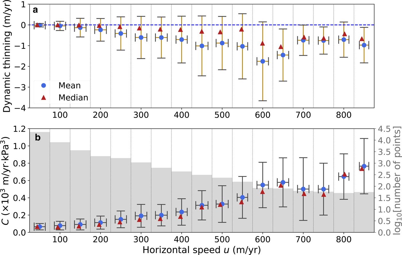
Fig. 8. Dynamic thinning rates and glacier characteristics. (a) Modeled changes in inland dynamic thinning rates (shown in map view in Fig. 1b) and (b) inferred basal slipperiness parameter C versus modeled horizontal flow speed u. In both panels, values are taken at the nodes of the finite element mesh and are binned by horizontal speed every 50 m a⁻¹. Bin boundaries are shown by vertical dotted lines, and gray bars in (b) indicate the number of points per bin on a log scale. Blue circles represent mean values, red triangles show median values, and error bars indicate one standard deviation about the mean.

3.2. Projections of dynamically driven mass loss

To examine how dynamically driven mass loss from BSS might change over approximately the next decade, we followed the same procedure as in the previous section, but we calculated the total expected ice-shelf thinning over the next 10 years, assuming that the mean ice-shelf thinning rates remain constant. After adjusting the ice-shelf thickness from the initialized state, ice-shelf thicknesses within our model domain remain above zero everywhere. The resulting changes in flow velocity are qualitatively similar to those shown in Figures. 1b, 7, and 8; thus we do not repeat the figures. Instead, we quantify the model results by simply noting that if ice-shelf thinning rates remain unchanged and the grounding line of George VI Ice Shelf remains fixed—as it approximately did from 1973 to 2010 (Holt and others, Reference Holt, Glasser, Quincey and Siegfried2013)—grounding line flux in BSS could increase by up to 13 Gt a⁻¹ before 2025. To estimate a plausible upper limit on mass loss, we increased ice-shelf thinning rates to three times the current values, reran the model, and found that grounding line flux could increase by as much as 30 Gt a⁻¹. These estimates of mass losses exclude contributions of grounding line retreat because we only apply thickness perturbations to freely-floating ice. More reliable projections of dynamically driven mass loss would require better constraints on bed topography than are currently available, allowing for realistic representations of the effects of grounding line retreat on dynamically driven mass loss in BSS.