


Introduction
The Arctic environment has been experiencing rapid changes over the past few decades (e.g. Richter-Menge and others, Reference Richter-Menge, Overland and Mathis2016). One of the most striking features is the dramatic reduction and thinning of the Arctic sea ice (e.g. Kwok and Untersteiner, Reference Kwok and Untersteiner2011; Cavalieri and Parkinson, Reference Cavalieri and Parkinson2012). In recent years, the rapid sea-ice retreat provides new opportunities for the navigation of commercial and scientific ships through the Arctic Routes, which significantly reduces the shipping distance from Asia to Europe. The increase in shipping activities in the Arctic, however, requires great efforts in improving the reliability of sea-ice forecasts (Jung and others, Reference Jung2016).
Examples of the state-of-the-art operational sea-ice and ocean forecasting systems are the Canadian Global Ice Ocean Prediction System (GIOPS; Smith and others, Reference Smith2016), the United States Navy Arctic Cap Nowcast/Forecast System (ACNFS; Hebert and others, Reference Hebert2015) and the Norwegian Tunable Optical Profiler for Aerosol and Ozone sea-ice/ocean numerical prediction system (TOPAZ4; Sakov and others, Reference Sakov2012). As an essential part to reduce the uncertainties associated with the initial states and external forcing, data assimilation has been widely applied in these operational systems to improve the prediction accuracy. The assimilation methods, however, are widely different in these prediction systems. For example, both GIOPS and ACNFS systems use a 3-dimensional variational analysis method, while TOPAZ4 applies an ensemble-based Kalman filter to assimilate the satellite and in-situ sea-ice and ocean observations.
For sea-ice observations, sea-ice concentration has been successively observed by several satellite passive microwave sensors during the past four decades (e.g. Cavalieri and Parkinson, Reference Cavalieri and Parkinson2012). Assimilating sea-ice concentration is hence the most common approach to initialize the sea-ice states in forecast models. The assimilation of sea-ice thickness observations is considered a further valuable source to reduce the uncertainties of the prediction systems. However, measuring sea-ice thickness from space is a challenge (Kwok and Sulsky, Reference Kwok and Sulsky2010; Kaleschke and others, Reference Kaleschke, Tian-Kunze, Maaß, Mäkynen and Drusch2012) and in-situ thickness observations are rather sparse. In recent years, datasets from the CryoSat-2 (Ricker and others, Reference Ricker, Hendricks, Helm, Skourup and Davidson2014) and Soil Moisture and Ocean Salinity (SMOS; Tian-Kunze and others, Reference Tian-Kunze2014) satellites have been validated against in-situ measurements, providing sea-ice thickness data in cold season. Following an optimal interpolation approach, these two thickness datasets have been combined to cover the entire Arctic region with a weekly frequency (CS2SMOS; Ricker and others, Reference Ricker2017). Model studies also show improved sea-ice thickness estimates when assimilating these two satellite datasets. For example, the assimilation of SMOS ice thickness significantly improves the first-year ice thickness estimates (Yang and others, Reference Yang2014, Reference Yang, Losch, Losa, Jung and Nerger2016a; Xie and others, Reference Xie, Counillon, Bertino, Tian-Kunze and Kaleschke2016), while joint assimilation of SMOS/CryoSat-2 ice thickness provides more reasonable sea-ice thickness estimates over the entire Arctic during a single cold season (Mu and others, Reference Mu2018b; Xie and others, Reference Xie, Counillon and Bertino2018). The joint assimilation has been further extended to the whole CryoSat-2 period to obtain a new sea-ice thickness record, the Combined Model and Satellite Thickness (CMST; Mu and others, Reference Mu2018a). A comprehensive evaluation against in-situ observations, satellite data and the widely used Pan-arctic Ice Ocean Modeling and Assimilation System (PIOMAS) data show the reliability of CMST (Mu and others, Reference Mu2018a). Although there are no available satellite-based sea-ice thickness observations in summer, the assimilation of the summer sea-ice concentration, with the multivariate data assimilation based on the ensemble Kalman filter, can help correct the modeled sea-ice thickness utilizing its covariance with the sea-ice concentration (Yang and others, Reference Yang, Losa, Losch, Jung and Nerger2015a, Reference Yang2016b; Mu and others, Reference Mu2018a). These provide us with a basis for a reliable sea-ice thickness prediction in summer.
For short-term environmental forecasts of the Arctic Ocean in support of the Chinese National Arctic Research Expeditions (CHINARE), a pan-Arctic sea ice–ocean forecasting system was configured in 2010 (Yang and others, Reference Yang2011, Reference Yang2012) at the National Marine Environmental Forecasting Center of China (NMEFC). The system uses a regional sea ice–ocean coupled model based on the Massachusetts Institute of Technology general circulation model (MITgcm; Marshall and others, Reference Marshall, Adcroft, Hill, Perelman and Heisey1997). To constrain the sea-ice initial conditions, satellite-retrieved sea-ice concentration data from Advanced Microwave Scanning Radiometer 2 (AMSR2) were assimilated into the forecasting system by nudging the modeled sea-ice concentrations toward the observations (Zhao and others, Reference Zhao2016). This simple approach has been validated to improve the sea-ice concentration forecasts, but the sea-ice thickness forecast remains unimproved.
In summer 2017, the Chinese icebreaker Xuelong successfully passed through the trans-Arctic Passage during the CHINARE 2017 Arctic Expedition. Since Xuelong is a class B1 icebreaker, only capable of continuously breaking ice thickness of 1.1 m, both accurate sea-ice concentration and thickness forecasts of the trans-Arctic Passage were required by the icebreaker at that time. To offer reliable Arctic sea-ice prediction, the original Arctic sea-ice prediction system was upgraded to a completely new forecasting system: the Arctic Ice Ocean Prediction System (ArcIOPS). In this new system, the same Arctic regional configuration of MITgcm and National Centers for Environmental Prediction (NCEP) Global Forecast System (GFS) forcing were kept, but the satellite sea-ice concentration and thickness observations were assimilated into the system with an advanced ensemble-based local error subspace transform Kalman filter (LESTKF; Nerger and others, Reference Nerger, Janjić, Schröter and Hiller2012). The real-time sea-ice forecast service for Xuelong occurred between 1 July and 30 September 2017.
In this paper, the sea-ice concentration and thickness forecasts for up to 5 days (120 hours) are evaluated with satellite and in-situ observations. A detailed description of the forecasting system and the data used for evaluation are presented in section ‘Model and data’, followed by the forecasting evaluation and results in section ‘Forecast evaluation’. Conclusions and discussions are provided in section ‘Conclusions and discussion’.
Model and data
Arctic Ice Ocean Prediction System (ArcIOPS)
The ocean and sea-ice components of ArcIOPS are based on the MITgcm sea ice–ocean model (Marshall and others, Reference Marshall, Adcroft, Hill, Perelman and Heisey1997). This model is configured regionally with a horizontal resolution of ~18 km and with the southern open boundaries around 55 N° (Losch and others, Reference Losch, Menemenlis, Campin, Heimbach and Hill2010; Nguyen and others, Reference Nguyen, Menemenlis and Kwok2011; Mu and others, Reference Mu, Zhao and Zhong2017). The viscous-plastic dynamics are used in the sea-ice model together with the zero-layer thermodynamics (Semtner Jr, Reference Semtner1976). To also parameterize thick ice growth in the sub-grid scale, seven thickness categories with a prescribed homogeneous distribution between 0 and 2H (H is the mean ice floe thickness) are used (Hibler III, Reference Hibler1979). The same approach is also applied to the snow. The subgrid scale ice thickness distribution is currently not used in the study. Parameters for the ocean and the sea-ice model are primarily optimized by Nguyen and others (Reference Nguyen, Menemenlis and Kwok2011), and thereafter are further tuned based on our configuration.
For operational forecasts starting at 12h, 12 instances of the sea ice–ocean model state are generated by ArcIOPS (Fig. 1). The ensemble models are initialized at 24 hours before as indicated by − 12h in Figure 1. During the initialization, sea-ice thickness data and sea-ice concentration data are assimilated into the model using the LESTKF as coded in the Parallel Data Assimilation Framework (Nerger and Hiller, Reference Nerger and Hiller2013, http://pdaf.awi.de).
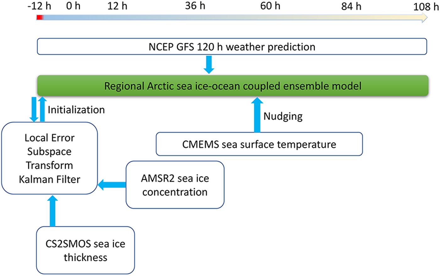
Fig. 1. The arctic ice ocean prediction system.
The CS2SMOS data are used for sea-ice thickness assimilation (V1.3; Ricker and others, Reference Ricker2017, http://data.meereisportal.de). The resolution of CS2SMOS thickness data is 25 km. Sea-ice thickness errors provided in CS2SMOS are considered as representative errors during analysis. The sea-ice concentration data with a resolution of 6.25 km are provided by the University of Bremen, which are retrieved from the brightness temperature collected by AMSR2 (https://seaice.uni-bremen.de/sea-ice-concentration/) using the ARTIST Sea Ice (ASI) algorithm (Spreen and others, Reference Spreen, Kaleschke and Heygster2008). A uniform value of 0.2 is assigned as its representative error based on hindcast experiments before the real-time forecast. Following previous studies, a radius of ~126 km (seven grids in our configuration) is applied to localize the analysis (e.g. Yang and others, Reference Yang2014). Note that the CS2SMOS thickness data are only available during the freezing season (i.e. no thickness assimilation after 9 April). Nevertheless, the CS2SMOS thickness assimilation from 1 January to 9 April already constrains the model thickness field toward the observation and provides reasonable initial states for further sea-ice prediction during the melt season (Allard and others, Reference Allard2018; Blockley and Peterson, Reference Blockley and Peterson2018).
The sea surface temperature of the ocean model is constrained by satellite observations (product SST_ARC_SST_L4_NRT_OBSERVATIONS_010_008_b, http://marine.copernicus.eu) from the Copernicus Marine Environment Monitoring Service with a simple nudging scheme. Because the near-real-time SST product available on the forecast day is actually already 2 days lagged. To take the potential effects into account, the relaxation coefficient used for nudging is further delicately tuned.
The state vector consists of sea-ice concentration and sea-ice thickness. Their background covariance matrix is dynamically generated and evolves during the assimilation. For a realistic ensemble spread, additional ensemble state perturbations are added every 7 days. The perturbations are prescribed as monthly fields calculated using the singular value decomposition method. Specifically, snapshots of sea-ice concentration and sea-ice thickness in each month from the previous 5 years' (2012–2016) simulation are collected and decomposed into empirical orthogonal functions (EOFs) after subtracting their mean state. Using a second-order exact sampling (Pham, Reference Pham2001), the perturbation takes the product of the leading 12 EOFs and a random matrix.
Downward shortwave radiation, downward longwave radiation, 2 m temperature, 10 m surface winds, precipitation and specific humidity from the NCEP GFS 120 hour atmospheric forecasts (https://www.ncdc.noaa.gov/data-access/model-data/model-datasets/global-forcast-system-gfs) are calibrated based on previous work Mu and Zhao (Reference Mu and Zhao2015), and used to drive the models. Considering the uncertainties from the single forcing (Yang and others, Reference Yang2015b), ArcIOPS utilizes a forgetting factor of 0.9 in LESTKF to increase the ensemble spread. During 120 hours' integration, ArcIOPS outputs ensemble forecasts of sea-ice concentration, sea-ice thickness, sea-ice drift and ocean fields. Note that all the forecasts have the same ensemble size of 12.
Data for evaluation
The sea-ice concentration product of the EUMETSAT Ocean and Sea Ice Satellite Application Facility (OSISAF; Eastwood and others, Reference Eastwood, Larsen, Lavergne, Nielsen and Tonboe2011) retrieved from the Special Sensor Microwave Imager/Sounder (SSMIS) (OSI-401-b) are used to evaluate the sea-ice concentration forecasts. This product is provided on the polar stereographic grid with a resolution of 10 km and is independent of the AMSR2 sea-ice concentration used for assimilation. The hybrid algorithm of the OSISAF data, which combines a Bootstrap algorithm in frequency mode (Comiso and others, Reference Comiso, Cavalieri, Parkinson and Gloersen1997) and the Bristol algorithm (Smith and Sandwell, Reference Smith and Sandwell1997), is in fact different from the ASI algorithm (Spreen and others, Reference Spreen, Kaleschke and Heygster2008) used for AMSR2. The satellite sensors on board are also different between these two products.
For sea-ice thickness evaluation, in-situ observations from Beaufort Gyre Exploration Project (BGEP) upward-looking sonar (ULS) moorings are used. The error of the ice draft in ULS measurement is about 0.1 m (Melling and others, Reference Melling, Johnston and Riedel1995). The sea-ice draft measured by the ULS is converted to thickness by multiplying with a factor of 1.1 (Nguyen and others, Reference Nguyen, Menemenlis and Kwok2011). Due to the absence of sufficient information about different ice types, ice densities and snow loading, uncertainties will be introduced during the conversion, however, they are ignored in the study.
The ice mass balance (IMB) buoys provide a Lagrangian specification of sea-ice evolution. The acoustic sounder above ice and the underwater sonar altimeter below ice measure the sea-ice changes simultaneously. The uncertainty of sea-ice thickness measured by each acoustic sounder is within 5 mm (Richter-Menge and others, Reference Richter-Menge, Overland and Mathis2016). Note that the information provided by the IMB buoys is ambiguous, to some extent, when compared to model results that are usually based on the Eulerian frame. We collect six IMB buoys data during Xuelong's transit through the trans-Arctic Passage: the IMB_2017B from the CRREL-Dartmouth Mass Balance Buoy Program (Perovich and others, Reference Perovich2013), the IMB_TUT78180 and the IMB_TUT78210 from the Taiyuan University of Technology (TUT), the IMB_FMI06 and the IMB_FMI18 from the Finnish Meteorological Institute (FMI) and the IMB_NMEFC from the National Marine Environmental Forecasting Center (NMEFC).
Sea-ice thickness data (v2.1) from the PIOMAS (Zhang and Rothrock, Reference Zhang and Rothrock2003) are also used in the study. The PIOMAS is forced by the NCEP/NCAR reanalysis. Sea surface temperature from the NCEP/NCAR Reanalysis and sea-ice concentration from National Snow and Ice Data Center (NSIDC) are assimilated into the model using nudging and optimal interpolation methods (Zhang and Rothrock, Reference Zhang and Rothrock2003; Schweiger and others, Reference Schweiger2011). The PIOMAS sea-ice thickness data have been widely used as a reference dataset for Arctic sea-ice thickness comparisons.
The ship-based ASPeCt (http://aspect.antarctica.gov.au) sea-ice thickness observations were conducted every half hour during Xuelong's transit through the trans-Arctic Passage. Such kind of observations shares the same protocol for sea-ice observing, which provides a standard and quantifiable method to further facilitate the analysis and comparisons with model results. It is well described in Worby and others (Reference Worby2008): ‘In the AsPeCt protocol, the ship-based observations are typically recorded hourly and include the ship's position, total ice concentration and an estimate of the areal coverage, thickness, floe size, topography, and snow cover characteristics of the three dominant ice thickness categories within a radius of approximately 1 km around the ship.’ One still needs to be aware that artificial uncertainties exist when comparing such data with model results. Because the ship would avoid ridged and thicker ice during transit and, as a result, the sea-ice thickness is underestimated in general. In particular, Xuelong can only continuously break ice as thick as 1.1 m (including 0.2 m thick snow) at a sailing speed of 1.5 knots (https://en.wikipedia.org/wiki/MV_Xue_Long). In this study, model results are interpolated onto Xuelong's trajectory in terms of the time-varied locations.
Forecast evaluation
The real-time forecasts start at 12:00 Beijing time (04:00 UTC) each day. ArcIOPS downloads the satellite sea-ice observation data and prepares necessary run-time model files automatically. Using 32 CPUs, the system can finish the ensemble forecasts in 2 hours. A typical forecasting product is shown in Figure 2. The sea-ice concentration, sea-ice thickness and drift forecasts were provided to Xuelong for shipping route decisions when transiting in sea-ice-covered area at that time. The valuable forecasting information had facilitated Xuelong's transit through the trans-Arctic Passage (Bing Zhu, Captain of Xuelong, personal communication, 2017). As shown in Figure 2, the actual transit route was basically along the forecasted ice thickness isoline of 1.5 m.
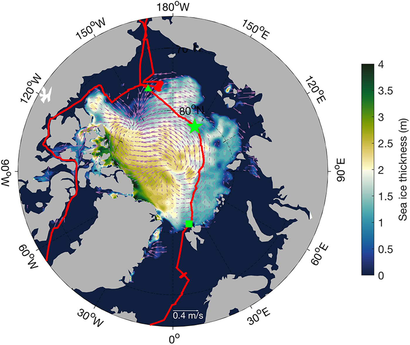
Fig. 2. 72 hour forecasts of sea-ice thickness and drift on 9 August 2017. The red curve shows Xuelong's trajectory during CHINARE2017. The green triangle in the Beaufort Sea indicates Xuelong's position on 2 August before it transited through the trans-Arctic Passage, and the green square indicates its position on 18 August when it was leaving the ice area. Xuelong's location on 9 August is indicated by the green star.
Sea-ice concentration
Due to different satellite sensors and to the different algorithms used during the retrieval, sea-ice concentration products show remarkable deviations (Ivanova and others, Reference Ivanova2015). A paradigm on 2 August 2017 in Figure 3c demonstrates that the deviations can easily reach as high as 0.5 in the marginal ice zone (MIZ). The AMSR2 sea-ice concentration is generally higher than OSISAF SSMIS. The SSMIS data with a resolution of 10 km are smoother compared to the AMSR2 data that are provided on a relatively higher resolution (6.25 km) (Figs 3a, b). As a result of assimilating AMSR2 concentration, ArcIOPS sea-ice concentration forecasts at different leading times are higher than SSMIS data (Figs 3d, e, f). The sea-ice concentration near the ice edge in the Beaufort Sea is also higher than both AMSR2 and SSMIS. However, when compared to AMSR2, even the 120 hour forecast is able to well capture the spatial distribution of sea-ice concentration (Figs 3a, f).
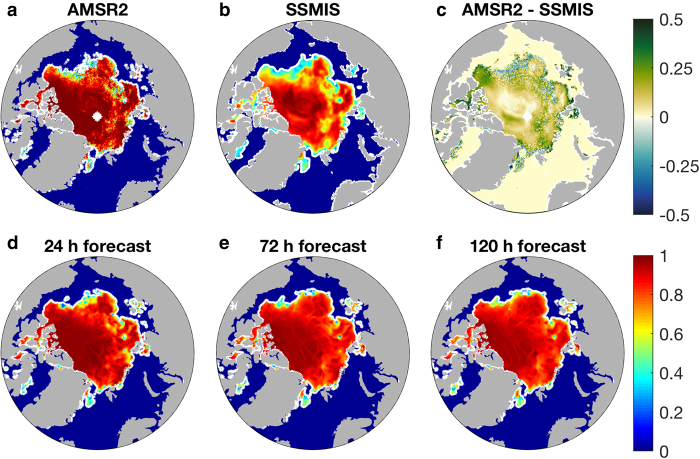
Fig. 3. Sea-ice concentration on 2 August 2017. Note that sea-ice concentration from AMSR2 (a) and OSISAF SSMIS (b) share the same color bar with the plots of the forecasts (d, e, f). The differences (c) between AMSR2 and SSMIS are computed with both data downscaling onto the model grids. The sea-ice concentration field ranges from 0 to 1, and the contour lines of 0.15 are plotted in white in all the subplots apart from (c).
In the RMSE calculation, for example, Lisæter and others (Reference Lisæter, Rosanova and Evensen2003) calculated the value over the area where either the modeled or the observed concentration is higher than 0.05. For sea-ice concentration from AMSR2, SSMIS and forecasts, the area where any data product is above 0.05 and below 0.8 (Strong, Reference Strong2012) covers the MIZ and also the ice floe area near the ice edge. In such areas, sea ice will be significantly influenced by oceanic processes (e.g. ocean waves and tides). Hence, statistics over this area take these processes into account. Meanwhile, we also calculate the RMSE over the area where any data products are above 0.8, which generally represents the system performance over the compact ice area.
From July to September, for both OSISAF and the ArcIOPS forecasts in the MIZ, the calculated RMSEs with respect to AMSR2 first decrease and then increase as new ice formation starting from 1 September (Fig. 4a). The performances of the forecasts degrade from 24 to 120 hours as expected. However, the RMSE of the 24 hour forecast is lower than that of OSISAF, meaning that it still lies within the observation uncertainty range. OSISAF data have roughly the same performance with the 72 hour forecast. Statistical analyses (Fig. 4a) confirm this with the mean RMSEs of 0.34 0.32, 0.34, and 0.36 for OSISAF, 24, 72 and 120 hour forecasts, respectively.
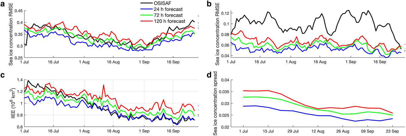
Fig. 4. Sea-ice concentration RMSE (a, b), IIEE (c) and sea-ice concentration spread (d) from 1 July to 29 September over the model domain. The 24, 72, and 120 hour leading forecasts are shown in blue, green and red, respectively. RMSE between AMSR2 and OSISAF SSMIS is shown in black. Note that (a) is computed over the area where any data are larger than 0.05 and below 0.8 with respect to AMSR2 data, and (b) is computed over the area where any data are larger than 0.8. IIEE is calculated with respect to AMSR2 data. Also note that on 28 September, data gaps are found in the AMSR2 sea-ice concentration data. The sea-ice concentration spread defined as the ensemble standard deviation in (d) is the weekly mean calculated over the ice area.
Over the compact ice area, however, all the data show slight declining trends for this period (Fig. 4b). RMSEs for OSISAF, 24, 72 and 120 hour forecasts are 0.10, 0.05, 0.06 and 0.07, respectively. The RMSEs of ArcIOPS forecasts are all lower than OSISAF. The assimilation of AMSR2 data gives rise to this result over the compact ice area, but it is not the case in Figure 4a, where large deviations exist between AMSR2 and OSISAF in the MIZ as also found in Figure 3.
The integrated ice-edge errors (IIEE; Goessling and others, Reference Goessling, Tietsche, Day, Hawkins and Jung2016) with respect to AMSR2 are also calculated as shown in Figure 4c. The shrinking ice edge from July to September is well illustrated by this metric in all the data. IIEE of OSISAF is generally larger than 24 and 72 hour forecasts in July but converges to that of 24 hour forecast from 1 August. It demonstrates that the 24 hour ice edge forecast is reliable and it also lies within the deviation range between two different satellite observations. The sea-ice concentration spread, hereinafter defined as the ensemble standard deviation, shares the same evolution as the IIEE (Fig. 4d). The mean spreads for each forecast over this period are 0.025, 0.029 and 0.030, which are within the range as shown in Yang and others (Reference Yang, Losa, Losch, Jung and Nerger2015a). The spatial distribution of the spread is generally consistent with RMSE with respect to both AMSR2 and SSMIS (figure not shown).
Given the discussion above, the ArcIOPS exhibits good forecast skill on 24 hour sea-ice concentration forecast both in the MIZ and over the compact ice area. The same conclusion also emerges from the statistics using OSISAF as the reference data (figure not shown).
Sea-ice thickness
The remotely sensed observations of ice thickness from satellites are unavailable in summer, because the state-of-the-art retrieving algorithms are impeded by the saturated surface water vapor from surface snow melting (Ricker and others, Reference Ricker, Hendricks, Helm, Skourup and Davidson2014). In-situ observations, however, are rather rare. The ASPeCt-based observations, albeit have large uncertainties and gaps, but represent the most comprehensive insights on sea-ice properties, and they have been widely used in literature for decades (e.g. Worby and Allison, Reference Worby and Allison1999; Worby and others, Reference Worby2008; Haumann and others, Reference Haumann, Gruber, Münnich, Frenger and Kern2016). It is also worth pointing out that these ASPeCt observations are not assimilated in ArcIOPS during the forecast. The model thickness used hereinafter is the effective thickness unless otherwise specifically stated.
As the comparisons to ASPeCt observations showing in Figure 5, the ArcIOPS forecasts have predicted reasonable sea-ice thickness during Xuelong's transit through the trans-Arctic Passage compared to PIOMAS. The fluctuations of ASPeCt observations on 2 August are expected because at that time Xuelong just sailed into the sea-ice edge area from the open water. Large differences are found on the last day (18 August) between ASPeCt observations and other data sources, this is also expected, because at that time Xuelong was navigating north of Svalbard Islands and was leaving the pack ice area.
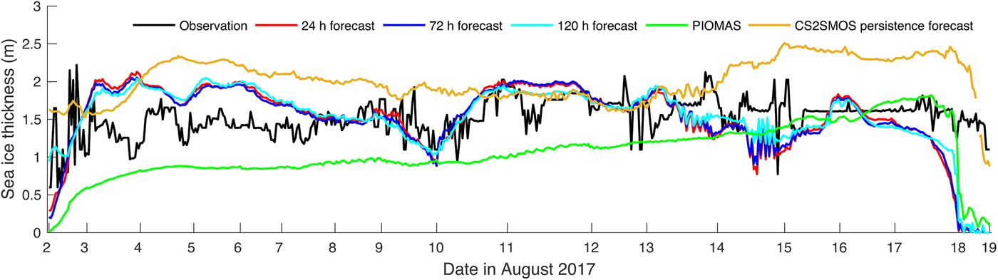
Fig. 5. ArcIOPS sea-ice thickness forecast (red line for 24 hour forecasts, blue line for 72 hour forecasts and cyan line for 120 hour forecasts) during Xuelong's transit through the trans-Arctic Passage. The ASPeCt observations aboard Xuelong are shown in black. PIOMAS results are shown in green. The CS2SMOS persistence forecast indicated in orange shows the last CS2SMOS thickness record before the forecast on 9 April. Note that all these comparisons are conducted along Xuelong's route from 2 August to 19 August.
The mean sea-ice thickness during the transit period for ASPeCt-based observation is 1.53 m, that for ArcIOPS forecasts are 1.53 m (24 hour forecast), 1.52 m (72 hour forecast) and 1.55 m (120 hour forecast). PIOMAS underestimates the ice thickness with a mean value of 1.06 m. The persistence forecast from CS2SMOS apparently cannot accurately predict the sea-ice melting, but it is still shown as a reference in Figure 5. It is worth noting that the performance of 120 hour forecasts has minor differences from other forecasts (i.e. 24, 72 hour forecasts). Student's t-test also reveals that such differences are not statistically significant. This is because the sea-ice thickness evolution in Figure 5 reflects not only temporal variations but also spatial variations along Xuelong's trajectory. The spatial distribution of sea-ice thickness is initialized by assimilating CS2SMOS thickness and evolves by model dynamics. Although there are no CS2SMOS thickness data available after April, the realistic spatial distribution of ice thickness persists over the melting period and hence is conducive to the better prediction in summer. From the temporal perspective, this is also because sea-ice thickness melting is rather small in 5 days (120 hour), and the effects on ice thickness forecast due to differences between the 24 and 120 hour atmospheric forecasts can be negligible in ArcIOPS. Meanwhile, the thickness corrections from sea-ice concentration assimilation are relatively small in such thick ice areas because the saturation of the sea-ice concentration (~0.8) leads to minor thickness updates. Apparent differences between 24 and 120 hour forecasts can be found in the thin ice area and over long-term integration (figure not shown). Besides, the model resolution we used in the study could generate further mismatches, because the coarse model smooths sharper variations that could be introduced by other players, e.g. the GFS forcing or the sea-ice concentration assimilation with higher resolution products.
The histogram of sea-ice thickness further confirms that ArcIOPS forecasts have better performances than PIOMAS reanalysis over the transit (Fig. 6). PIOMAS overestimates the thin ice thickness (< 1.5 m), while ArcIOPS forecasts underestimate ice thickness within the bin 1.5–1.75 m, and overestimate within the bin 2.0–2.25 m. Note that the ASPeCt observations may underestimate thicker ice because the ship would tend to circumvent thick and ridged ice regions, which could distort its histogram within thick bins. This overestimation in PIOMAS appears to be persistent starting from the freezing season as illustrated in Mu and others (Reference Mu2018a). The ArcIOPS 120 hour forecasts are closer to the ASPeCt than the 24 and 72 hour forecasts. That uncertainties that exist both in the observations and the atmospheric forcing makes this rather arguable. Figures 5 and 6 demonstrate that when it comes to the spatial distribution of sea-ice thickness in the Arctic, forecasts with 5 days lead time are conceivable.
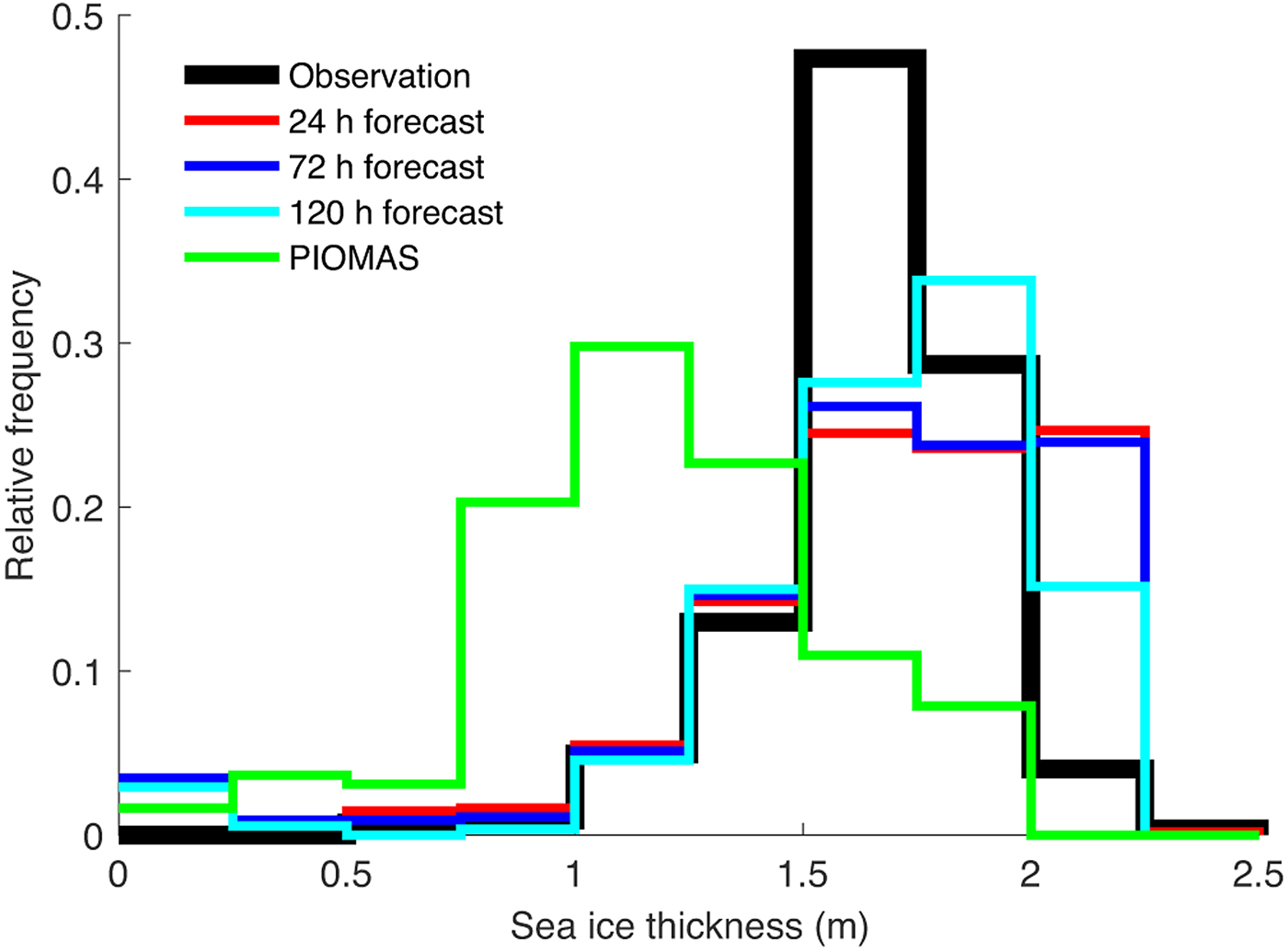
Fig. 6. Histogram of sea-ice thickness of each data during Xuelong's transit through the trans-Arctic Passage from 2 August to 19 August. The ASPeCt observations aboard Xuelong are shown in black. The 24, 72, and 120 hour forecasts are shown in red, blue and cyan, respectively. PIOMAS data are shown in green.
Further evaluations are conducted by comparing the forecast results with in-situ observations during and after the transit. The model results are interpolated onto the ULS locations or onto the IMB trajectories for these two different types of observations. It is worth noting that the effective sea-ice thickness from ArcIOPS and PIOMAS are compared with ULS observations, while the ice floe thicknesses are used for comparisons with IMB observations. Comparisons to ULS mooring thickness data at BGEP_A, BGEP_B and BGEP_D (Fig. 7b) show that the 24 hour forecast has smaller biases than the 72 and the 120 hour forecasts (Fig. 7a). The declines of the sea-ice thickness are delayed as shown from the 24 to the 120 hour forecasts at BGEP_B and BGEP_D. This reflects the delayed synoptic phenomenon in the atmospheric forcing. The statistics in Table 1 support the impression that the 24 hour forecast tends to perform better. At BGEP_A and BGEP_B, the 24 hour forecast fits better to observations, with RMSEs of 7.2 and 10.4 cm, while at BGEP_D, PIOMAS thickness is closer to the observation with a RMSE of 9.1 cm. The mean errors (ME) points to the same conclusion, apart from at BGEP_B where the 120 hour forecast has lower ME than the other two.
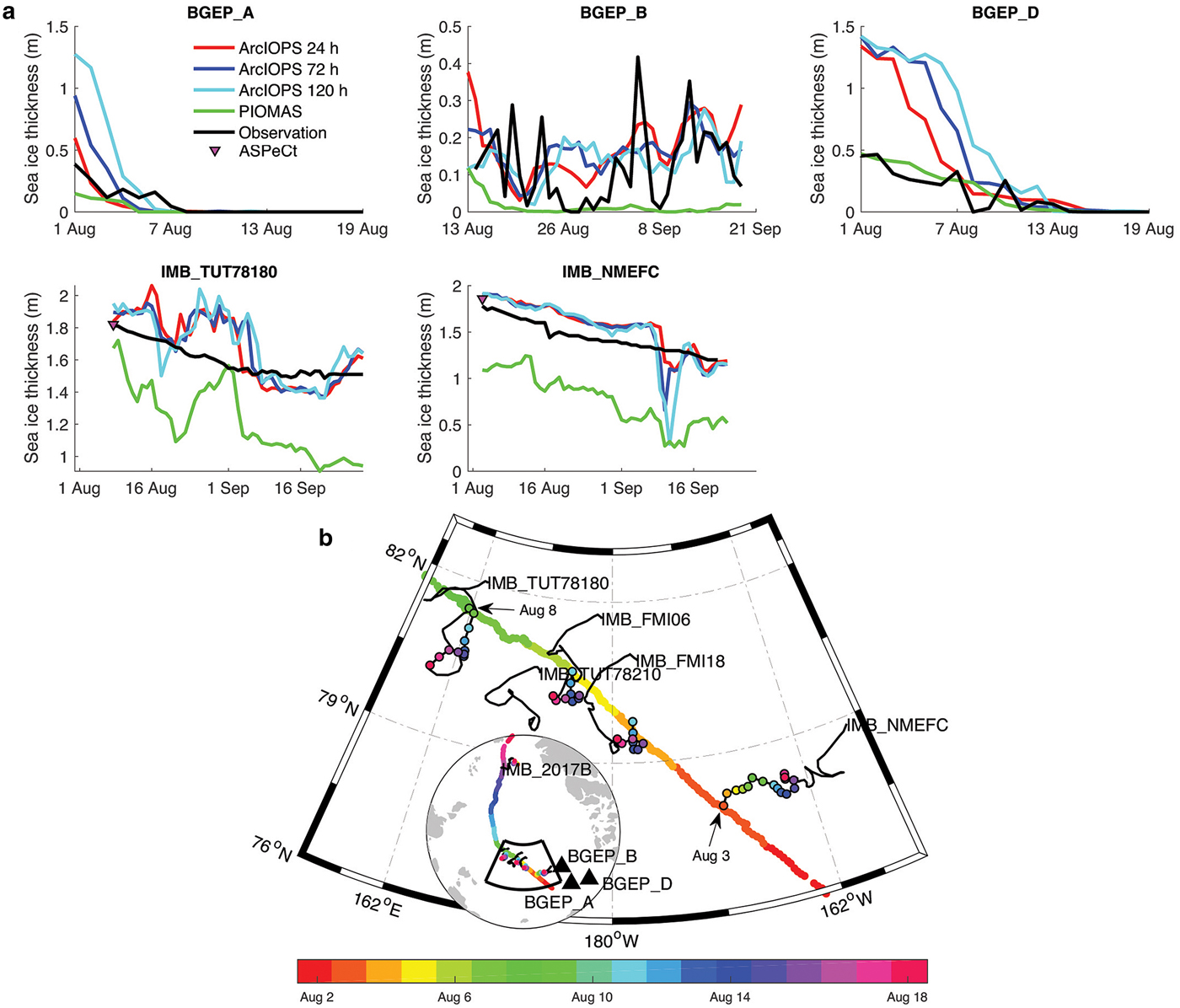
Fig. 7. Comparisons to in-situ sea-ice thickness observations when ice exists during August and September in 2017 (a). Observations are shown in black. ArcIOPS 24, 72, and 120 hour forecasts are shown in red, blue and cyan, respectively. PIOMAS sea-ice thickness is shown in green. Locations of BGEP ULS (black triangles) and trajectories of IMBs are shown in subplot (b). Trajectories of Xuelong and IMBs are dotted in color indicating both location and the current date with the color bar below showing dates in different colors. The coincident date between ASPeCt and IMB observations are indicated by arrows, and the ASPeCt ice floe thickness observations are shown by inverted triangles in (a). Note that the background plot in (b) is an enlarged version of the foreground plot.
Table 1. Sea-ice thickness statistics of ArcIOPS forecasts and PIOMAS with respect to observations over the periods in Figure 7a

Note that statistics for ULS moorings are calculated when all the data have sea ice. RMSE (cm) is the root-mean-square-error; ME (cm) stands for the mean error; S (cm) is the ensemble spread.
The collected IMBs are shown in Figure 7b. Comparisons between model results to IMB observations are not such straightforward because the representativity of the IMB observation for large areas is somewhat arguable. To reach robust conclusions, we divide six IMBs into two groups. One group is IMB_2017B, IMB_TUT78210, IMB_FMI06 and IMB_FMI18; the other is IMB_TUT78180 and IMB_NMEFC. The second group is used for evaluation. The reason is that in the first group, there are no further independent observations to support robust conclusions. IMBs in this group do not coincide with Xuelong's trajectory shown in Figure 7b. However, in the second group, the ship-based ASPeCt observations can serve as independent observations, because there are coincidences on the IMB trajectories and Xuelong's trajectory (Fig. 7b). For IMB_TUT78180, the intersection was on 8 August, and for IMB_NMEFC, it was deployed not far away from Xuelong on 3 August.
As shown in Figure 5, on the intersection of Xuelong and IMB_TUT78180's trajectories on 8 August, the ArcIOPS forecasts agree very well with ASPeCt observations, and both have an effective thickness of 1.5 m (ice floe thickness of ~1.8 m). At the same time, ice floe thickness differences among IMB_TUT78180, 24 hour ArcIOPS forecast and PIOMAS are not large (1.81, 1.83 and 1.67 m, respectively) (Fig. 7a), which confirms that IMB_TUT78180 observations can be reliably compared with model results. And hence, we can further assume the persistence of this reliability all over the drift period (Lei and others, Reference Lei2014). This is also the case for IMB_NMEFC that as an independent observation ASPeCt also validates this IMB's qualification for the comparison. The coincidence took place on 3 August when an ice station was conducted near Xuelong, which can be also found in Figure 5 where thicknesses have peak values during this day. The sea-ice thickness observations from IMB_NMEFC and ASPeCt are quite close with 1.70 and 1.78 m.
Sea-ice thickness from ArcIOPS forecasts is closer to observations than PIOMAS on IMB_TUT78180's trajectory (Fig. 7a). RMSEs for 24, 72 and 120 hour forecasts with respect to IMB_TUT78180 are 14.9, 15.1 and 16.9 cm, respectively, while that for PIOMAS is 38.9 cm (Table 1). The MEs for ArcIOPS forecasts and PIOMAS in Table 1 show that ArcIOPS overestimates the thickness (> 6.6 cm) while PIOMAS underestimates the thickness (− 38.5 cm). On IMB_NMEFC's trajectory, ArcIOPS generally overestimates the thickness with MEs larger than 6.0 cm, but underestimates the thickness around 11 August. Large biases with a ME of about 0.67 m are found in PIOMAS thickness. RMSEs of ArcIOPS forecasts with respect to IMB_NMEFC are 17.0 cm (24 hour forecast), 18.9 cm (72 hour forecast) and 24.6 cm (120 hour forecast), all lower than that of PIOMAS (~0.66 m).
To test whether the differences between the forecasted thicknesses in Figure 7a are statistically significant, the Wilcoxon rank-sum test is applied to handle the non-normal continuously distributed time series. Under the null-hypothesis, the distributions and medians of two forecasts are not significantly different. For p-values below 0.05 the null-hypothesis can be rejected, which are shown in italics in Table 2. The statistics show that 24 and 120 hour forecasts are significantly different, with a 95% confidence level at BGEP_D, and for IMB_TUT78180 and IMB_NMEFC. The differences between 24 and 72 hour forecasts are also significant at BGEP_B and for IMB_NMEFC. At BGEP_A, no significant differences are found among the forecasts. Sea-ice thickness ensemble spreads of the 24 hour forecasts are smaller than that of 72 and 120 hour forecasts. However, the ice thickness RMSEs with respect to the observations are at least twice as large as the ensemble spread. This confirms that systematic errors exist in the model. Further calibrations of model parameters and of the atmospheric forcing are warranted.
Table 2. The p-values of the Wilcoxon rank-sum test for sea-ice thickness forecasts over the periods in Figure 7a

The forecasts that show statistically significant differences (p < 0.05) are shown in italics.
Conclusions and discussion
Driven by the scientific interest on Arctic sea-ice predictability and also the increasing commercial demands on Arctic shipping, the ensemble-based Arctic sea ice–ocean prediction system ArcIOPS was developed. The forecasts had been utilized for the first time when Xuelong transited through the trans-Arctic Passage of the Arctic Ocean in summer 2017.
The evaluations demonstrate that the Arctic sea-ice forecasts from the first version of the operational ArcIOPS are convincing. Compared to the independent OSISAF SSMIS sea-ice concentration and also to the AMSR2 data, the RMSEs of ArcIOPS 24 hour forecast ice concentration are below the deviations between these two different satellite data products both in the MIZ as well as over compact ice areas. The 24 hour IIEE and RMSEs are also within the satellite observation errors. Furthermore, it should be stressed that the ArcIOPS sea-ice thickness forecasts perform better than PIOMAS sea-ice thickness compared to the ship-based ASPeCt, two ULS moorings (BGEP_A and BGEP_B) and also to the available IMB observations. However, ArcIOPS overestimates the sea-ice thickness as well as the concentration in the Beaufort Sea.
This study shows the importance of implementing the -ice thickness assimilation in current operational forecasting systems. Although the CS2SMOS sea-ice thickness data in summer are not available, the initialization in late April using satellite thickness data is beneficial to achieve sea-ice forecast improvement during melting season. Besides, the assimilation of sea-ice concentration in summer also helps to correct sea-ice thickness by means of their covariances. These covariances are found to be generally positive and gradually effective over the whole Arctic when sea ice is melting (figure not shown). The monthly mean covariances in summer over the whole Arctic can be ~4 times larger than that in freezing season. However, these covariances are calculated based on our model ensemble with a relatively small ensemble size (12). A larger ensemble may provide a more realistic covariance for this system. Better performances on sea-ice thickness are expected if PIOMAS would also assimilate the thickness data.
The satellite sea-ice concentration products also show large deviations in MIZ. They apparently have direct impacts on the assimilation. Concurrently, if the ensemble spread is not sufficiently large, overestimations of the sea-ice concentration and further the thickness are not surprising. Therefore, it is of great demand to study the potential effects when assimilating different sea-ice concentration products in each forecast system. More in-situ observations (ASPeCt, aerial observations) should be used to calibrate the system.
Motivated by this encouraging results, the second version of ArcIOPS with sea surface temperature assimilation is under development and will be put into operational use in the near future. To minimize current deficiencies in the system found in the study, more delicate bias correction and parameter tuning for the model and also for the assimilation will be applied in the new version.
Acknowledgments
This is a contribution to the Year of Polar Prediction (YOPP), a flagship activity of the Polar Prediction Project (PPP), initiated by the World Weather Research Programme (WWRP) of the World Meteorological Organisation (WMO). We acknowledge CHINARE 2017 for conducting the ship-based ASPeCt observation. This study is supported by the National Key R&D Program of China (2018YFA0605901), the National Natural Science Foundation of China (41776192 and 41706224), the Key Research Program of Frontier Sciences of CAS (QYZDY-SSW-DQC021), the Opening fund of State Key Laboratory of Cryospheric Science (SKLCS-OP-2019-09) and the Federal Ministry of Education and Research of Germany in the framework of SSIP (grant 01LN1701A). We thank colleagues from NMEFC and Taiyuan University of Technology for providing the in-situ observation data, and two anonymous reviewers for their constructive suggestions. We thank Lorenzo Zampieri and Bimochan Niraula for their efforts on improving the paper.


 Open access