

Polluting industries fear inspection teams. The problem is that it’s like a cat and mouse game. Each Tom has many Jerrys to catch, and Jerrys don’t behave when Tom’s not around.
Given the unambiguous nature of SO2 emissions control, adjusting the incentive structure has the potential to foster more consistent policy implementation during a leader’s tenure. In this chapter, I apply the theory of the political regulation wave to China’s SO2 control between 2001 and 2010. While the 10th FYP (2001–5) failed to clearly define how local leaders’ environmental performance would be evaluated, as well as the consequences of such evaluation, the 11th FYP (2006–10) unequivocally tied a leader’s promotion to reaching established environmental targets – SO2 reduction targets became mandatory and binding. Using both official and satellite-based data, I show that top leaders of prefectures with high reduction targets, acting on their career incentives, switched from gradually loosening enforcement to maintaining relatively consistent enforcement during their tenures. Thus, local political incentives can be a potent source of systematic local policy waves.
The chapter is organized as follows. I will first provide background information on SO2 control policy directives and measures. Then I will provide a recap of the empirical implications for SO2 emissions regulation based on the political regulation wave theory. I will lay out the research design, discuss empirical findings, and conclude the chapter with a summary of the results and the conditions under which a political environmental protection wave can be expected.
4.1 SO2 and Its Control Policies: Directives and Measures
There are eight major types of environmental pollution: air pollution, water pollution, land/soil pollution, noise pollution, radioactive/nuclear pollution, thermal pollution, light pollution, and marine/ocean pollution. Air pollution is the presence of different air pollutants, including but not limited to SO2, NO2, and PM (Figure 4.1).

Policymakers in China have long regarded SO2 as a major air pollutant. The extensive use of coal and other fossil fuels contributed to a prodigious amount of SO2 and NO2 emissions, which contributed to acid rain. As shown in Eqs. (4.1) and (4.2), the chemical process works as follows. SO2 and NO2 become transformed in the atmosphere to form gaseous sulfuric acid (H2SO4) and nitric acid (HNO3) respectively. These acids are then deposited on the land, forests, and water bodies via either dry acid deposition – the direct deposit of those acid gases on surface areas – or wet acid deposition, which involves acid gases dissolving in rainwater (acid rain), fog water (acid fog), or forming liquid aerosol particles (Reference JacobsonJacobson 2012, 221).
 (4.1)
(4.1)
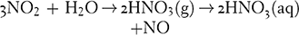 (4.2)
(4.2)
The acid deposition was particularly rampant in southern and southwestern China, where the sulfur content in coal reached as high as 4 percent, and the amount of alkaline dust – both natural (e.g., windblown dust from deserts) and anthropogenic (e.g., coal combustion, cement production, construction activities) – was insufficient to neutralize the acids (Reference Larssen, Lydersen, Tang, He, Gao, Liu and DuanLarssen et al. 2006, 419). These acids damaged buildings, agriculture, forests, among other types of surface areas. When inhaled in high concentrations, acids can be harmful to humans and animals. The costs of acid rain were estimated at USD 13 billion by China’s State Environmental Protection Administration (SEPA). The World Bank estimated USD 5 billion worth of damage to forests and agriculture and the human health costs to be around USD 11–32 billion, depending on the valuation method (Reference Larssen, Lydersen, Tang, He, Gao, Liu and DuanLarssen et al. 2006, 423). Acids and their precursors can travel across political boundaries, creating regional air pollution problems as happened in the southwestern region of China.
Reducing SO2 has been a policy priority in the realm of environmental protection since the 1990s. The 9th FYP (1996–2000) set limits on total SO2 emissions. In 1998, the State Council approved and SEPA rolled out the Two Control Zones (TCZ, 两控区) policy, officially known as The Acid Rain Control Zone and the Sulfur Dioxide Control Zone Partition Plan (酸雨控制区和二氧化硫污染控制区划分方案) (SEPA 1998). The SO2 Control Zone covers some cities in northern China while the Acid Rain Control Zone covers some cities in southern China. These cities under the TCZ policy, occupying about 11 percent of China’s land area, contributed to about 60 percent of total SO2 emissions. The 1998 TCZ policy sought to reduce (unsuccessfully) SO2 emissions, which was at 23.7 million tons in 1995, to 24.6 million tons in 2000. The policy also envisioned the 2010 emissions level being lower than that in 2000 and that cities under the TCZ would meet the national SO2 concentration standard of 60 µg/m3 or below. The 10th FYP put forward further SO2 total emissions control policies to work concurrently with the 1998 TCZ policy. Nevertheless, those policies only had a small and ephemeral effect on SO2 emissions reduction. Since 2002, the emissions level began climbing back, which prompted the central government to take new action.
After the 10th FYP, China’s SO2 regulation policy underwent a significant shift. Whereas SO2 emissions reduction targets had not been binding and were inadequately enforced during the 10th FYP, the advent of the 11th FYP saw the introduction of several policy instruments aimed at more stringent regulation of the pollutant. Interestingly, even though both five-year periods enjoyed healthy economic growth, and the central government had stipulated the same SO2 reduction targets for each, the 10th FYP period saw a 28 percent increase in SO2 emissions, while the 11th FYP led to a 14 percent reduction (Reference Schreifels, Fu and WilsonSchreifels, Fu, and Wilson 2012). The central government achieved this marked reversal in pollution outcomes by leveraging political and economic mechanisms that altered local leaders’ and polluters’ incentive structure and behavior.
With the 11th FYP, the central government made extensive political changes that induced the decline in SO2 emissions, most notable of which was the decision to explicitly tie local attainment of environmental targets to leaders’ prospects for promotion. Specifically, in 2006, the Central Committee of the Communist Party made the attainment of pollution reduction goals a hard criterion for promoting local leaders (Reference Schreifels, Fu and WilsonSchreifels, Fu, and Wilson 2012). Failure to meet such binding targets would constitute a failed tenure, which carried the risk of demotion – or even dismissal, in the event of severe lack of compliance. As emphasized in Chapter 3, local leaders are incentivized to fulfill binding policy targets and enforce regulation in such a pattern that is consistent with the perceived preferences of their superiors. With the advent of the 11th FYP, career-minded local leaders would have to prioritize SO2 reduction and regulate consistently during their tenure in order to score well on performance evaluations.
In addition to changing local leaders’ incentives, increased central monitoring and enforcement of existing policies helped reduce SO2 emissions. At the central level, the MEP narrowed the list of regulated pollutants to just SO2 and COD in order to devote more time and resources to their management. While the concept of total emission control (TEC) led previous FYPs to list numerous pollutants for regulation, more targeted efforts and monitoring during the 11th FYP significantly helped improve outcomes. Additionally, the MEP established two new departments charged with oversight of SO2 pollution levels: the Department of Total Emission Control and the Department of Environmental Monitoring.
At the local level, six regional supervision centers were established to make it easier for the MEP to supervise local governments and EPBs to prevent inaction, corruption, or failure to follow environmental guidelines and regulations. The central government also drastically increased the number of government employees involved in environmental monitoring. Between 2005 and 2008, the number increased from 46,984 to 51,753 – approximately a 10 percent jump (Reference XuXu 2011). Additionally, the number of government inspectors who conduct site inspections to ensure compliance with environmental regulations increased by nearly 20 percent, to 59,477, during the same period (Reference XuXu 2011). Thus, with enhanced monitoring capabilities and a higher likelihood of site inspections, the 11th FYP incentivized polluters to ensure they were in line with SO2 regulations.
Although less extensive than the political changes of the 11th FYP, the industry-intervention measures undertaken by the central government were of critical importance to curb SO2 emissions. For instance, small and inefficient coal-fired power plants were required to close, leaving in operation only large power plants that had the ability to control emissions more efficiently (Reference Price, Levine, Zhou, Fridley, Aden, Lu, McNeil, Zheng, Qin and YowarganaPrice et al. 2011). As a result, by 2010, the average coal consumed per kWh of electricity generated declined by 10 percent from 2005 levels (Reference Schreifels, Fu and WilsonSchreifels, Fu, and Wilson 2012).
The government also increased the pollution levy rate on emissions per ton. A pollution levy policy had already been in place for emissions above national standards since the 1979 Environmental Protection Law of the People’s Republic of China (for trial implementation) (中华人民共和国环境保护法 [试行]) (Standing Committee of the NPC 1979). However, the law had been inadequately enforced for a decade, and the levy itself remained too low to incentivize abatement. Since the levy was below the average emission control cost, firms would rather pay to pollute. The levy was progressively increased over time, to 0.42 RMB/kg (0.07 USD/kg) in 2003, 0.63 RMB/kg (0.10 USD/kg) in 2004, and finally 1.26 RMB/kg (0.20 USD/kg) in 2007, which was above the average emission control cost of around 1.2 RMB/kg (0.19 USD/kg) (Reference Schreifels, Fu and WilsonSchreifels, Fu, and Wilson 2012).
4.2 Empirical Implications for SO2 Regulation
The political regulation wave comes in two general patterns. When a pollutant does not have binding reduction targets, economic and stability goals trump environmental ones. Since political superiors expect gradual improvement in those critical goals, as documented in Chapter 3, we would expect to observe gradually laxer regulation of pollution throughout a given tenure, ceteris paribus. However, when that pollutant receives binding reduction targets tied to top local political leaders’ career prospects, we should expect to see more consistent regulation of that pollutant during a leader’s time in office, if the reduction of that pollutant is high conflict and low ambiguity. Such consistency is likely to be observed for SO2 because its reduction policy is unambiguous in both goals and means. The goal is to reduce SO2 emissions by 10 percent during an FYP. Achieving that goal is also unambiguous because SO2 is emitted primarily by the industrial sector, and containment requires installing and operating SO2 scrubbers. Furthermore, SO2 tends to stay close to its emissions source, which means that spillover from other jurisdictions is insignificant. As long as a given jurisdiction manages its SO2 emissions well, it does not have to be too concerned about dealing with others’ emissions.
We should expect to see that regulation relaxed gradually under the 10th FYP (2001–5) and remained relatively consistent during the 11th FYP (2006–10), especially for prefectures that received high reduction targets. Top leaders in those areas are more incentivized to order regulation in such a pattern that is consistent with the preference of the central government because they would not be able to explain away a significant lack of compliance, given high targets.
4.3 Research Design
The central puzzle this chapter seeks to tackle is: how do political incentives exercised through the local tenure time frame influence the political implementation of SO2 regulatory policies? It will speak to whether and how local political incentives can systematically shape the stringency of environmental regulation in the same prefecture over time, giving rise to systematic policy waves. The research design takes advantage of a policy initiative that made SO2 emissions reduction a binding target in the evaluation of local officials in most prefectures and thus changed the local incentive structure for environmental regulation. I gathered data from three sources: (1) City Statistical Yearbooks deposited online or housed at local archives and libraries, (2) Urban Statistical Yearbooks of China compiled by the National Bureau of Statistics, and (3) daily SO2 and NO2 observations retrieved from NASA’s ozone monitoring instrument (OMI).
The key dependent variable is regulatory stringency, proxied by two measures: (1) the SO2 removal ratio and (2) the ratio between NO2 and SO2. A common practice in the literature to measure the stringency of regulation of industries is to use the pollution discharge levy rate as a proxy. However, it does not work well for China because EPBs have been documented to possess and exercise discretion over the judgment of compliance and the amount of levy to collect. (Compliance can be conceptualized as the interaction between rules and behaviors.) Industrial compliance with environmental regulations, such as paying pollution levies, is far from universal, even in developed regions of North America (Reference Dasgupta, Huq and WheelerDasgupta, Huq, and Wheeler 1997). The compliance rates are usually lower in developing countries due to capacity constraints and inspector corruption. Underreporting and underassessment are commonplace among regulators (Reference Dasgupta, Huq and WheelerDasgupta, Huq, and Wheeler 1997). For instance, EPBs in China have been found to reduce, exempt, or postpone levy collection from financially insolvent factories that hire a substantial segment of the local labor force or from state-owned factories (Reference Dasgupta, Huq and WheelerDasgupta, Huq, and Wheeler 1997; Reference Wang, Mamingi, Laplante and DasguptaWang, Mamingi, et al. 2003; Reference TiltTilt 2007). Other contextual factors that shape those decisions include the severity of the local pollution problem and public complaints against the polluter, especially when covered by the media (Reference Wang, Mamingi, Laplante and DasguptaWang, Mamingi, et al. 2003; Reference TiltTilt 2007). In other words, regulators can bend the rules written on paper to suit particular circumstances at their discretion. Hence, it is necessary to use alternative measures to proxy for regulatory stringency.
For this study, I refer to both official and satellite-derived SO2 statistics. Official statistics blend reality and distortion of reality – what local leaders try to make their superiors believe about their performance. Local official statistics in China have largely been characterized as “dubious,” leading to the popular belief that “officials make statistics and statistics make officials” (官出数据, 数据出官). On the other hand, satellite-derived statistics are comparatively more objective and reflect reality better. Hence, it is an interesting exercise to compare the patterns revealed by official statistics with those that are satellite derived.
With regard to official statistics, SO2 removal ratio is an appropriate proxy for regulatory stringency. SO2 mainly comes from industry, and scrubbers are used to remove SO2 from flue gas. Due to SO2 scrubbers being expensive to maintain and operate, firms have been documented as operating their SO2 scrubbers consistently only when EPB regulators are onsite or when their chances of being onsite are high (Reference XuXu 2011). This is echoed in my field interviews (Interviews 0715CD03 and 0715CD04), in which one EPB chief humorously compared inspection teams and polluting industries to “Tom and Jerry.” “Each Tom has many Jerrys to catch, and Jerrys don’t behave when Tom’s not around,” said the chief. SO2 removal ratio is calculated based on Eq. (4.3). The annual SO2 emissions and removal statistics come from the Urban Statistical Yearbooks.
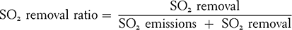 (4.3)
(4.3)
Based on satellite-derived statistics, I employ the ratio between two remotely sensed trace gases (
 ) to proxy for SO2 regulatory stringency. SO2 and NO2 are often generated from the same combustion processes, though that may vary by locality. Since NO2 was not a criteria air pollutant during 2001–10 but SO2 was, regulation by EPBs would center on the installment and operation of SO2 scrubbers. Data retrieved from NASA on NO2 and SO2 concentrations share the same measurement unit. Hence, the ratio of NO2-to-SO2 concentration reflects the operation of SO2 scrubbers and, by extension, the stringency of SO2 regulation. Appendix B provides more technical details on SO2 and NO2 characteristics and data.
The key explanatory variables are the “year in office” and its interaction with “post-2005” (Table 4.1). “Year in office” measures the number of years since the beginning of a leader’s time in office. For instance, “1” denotes being in office for the first year and “2” for the second year. In coding year in office, I follow the rule that if the leader exits from the post before June, that year is counted toward the successor. Conversely, if the leader leaves in or after July, that year is counted toward the leader. For political leaders serving a second five-year term on the same post, their years in office are coded continuously from the fifth year in the first term (e.g., sixth year instead of the first year during the second term) because leaders serving a second term are likely to be qualitatively different in terms of their experience, skills, aspirations, and their superiors’ expectations of them compared with the first time they served on the post. “Post-2005” is a dummy variable indicating whether the year for a prefecture-year observation in the dataset is after 2005.
Table 4.1 Summary statistics for observations from nonoverlapping tenures for prefectures that received high reduction targets
| Time period | Num. obs. | Min | Max | Median | Mean | Std. dev. | |
|---|---|---|---|---|---|---|---|
| Dependent variables | |||||||
| SO2 removal ratio | 2003–10 | 461 | 0.00 | 1.00 | 0.34 | 0.36 | 0.25 |

| 2005–10 | 351 | −87.50 | 383.03 | 1.06 | 1.68 | 22.58 |
| Independent variable | |||||||
| Year in office | 2001–10 | 614 | 1.00 | 9.00 | 2.00 | 2.45 | 1.46 |
| Control variables | |||||||
| Proportion of GDP from the industrial sector | 2001–10 | 693 | 0.17 | 0.89 | 0.46 | 0.46 | 0.11 |
| Proportion of industrial GDP from domestically owned enterprises | 2001–10 | 690 | 0.15 | 1.00 | 0.91 | 0.85 | 0.16 |
| Profitabilitya | 2001–10 | 692 | −1.01 | 12.18 | 1.90 | 2.03 | 1.09 |
| Log (capital intensity)b | 2001–10 | 689 | −1.16 | 6.48 | 0.27 | 1.21 | 1.95 |
Note: Figures are rounded to the second decimal.
a Profitability = profit / value-added.
b Capital intensity = total assets / sales volume.
I also include in Table 4.1 four industrial variables that are possibly correlated with the key explanatory variables and may also affect the SO2 removal ratio. Contributions of the industrial sector to the local economy, domestic ownership of firms, and firms’ financial solvency have been documented to influence regulatory stringency (Reference Dasgupta, Huq and WheelerDasgupta, Huq, and Wheeler 1997; Reference Wang, Mamingi, Laplante and DasguptaWang, Mamingi, et al. 2003; Reference TiltTilt 2007). Capital intensity measures the capital present in relation to other factors of production, especially labor. Generally speaking, the higher the capital intensity, the higher the labor productivity. Firm productivity may also be correlated with regulatory stringency. Further, all four factors could be correlated with the local political calendar. Thus, the control variables are the proportion of a prefecture’s GDP from the industrial sector, the proportion of industrial enterprises that are domestically owned, the profitability of the industrial enterprises, and the capital intensity of the enterprises.
Some tenures overlap the 2001–5 and tReference Hehe 2006–10 periods, comprising about 38 percent of the observations. Since the objective is to assess the temporal trend in regulatory stringency during a leader’s tenure under a FYP, I include only observations from nonoverlapping tenures, or tenures that fall entirely under a single FYP, for regression analysis. The summary statistics for observations for prefectures that received high targets, requiring reduction by 15 percent or higher (about 30 percent of all observations) are exhibited in Table 4.1.
4.4 Empirical Evidence
The goal is to measure how incentives provided by cadre evaluation shape regulatory patterns over time under two different FYPs. One big challenge in modeling this stems from the opacity of the criteria guiding SO2 reduction assignment; in other words, it remains unclear why some prefectures were assigned binding reduction treatment while others were not and why some prefectures received higher percentage reduction targets than others. Given the opacity surrounding the treatment assignment rule, difference-in-differences and matching methods could be potential solutions. Among the 252 prefectures in the dataset, 237 were treated for binding reduction targets and only 15 were not, rendering matching methods, like propensity score matching, ineffective. In addition, the pretreatment trends for the treatment and control groups are very different, so difference-in-differences does not apply either. Instead, I opt for evaluating the first difference of difference-in-differences (i.e., the before-and-after difference) among units in the treatment group while controlling for confounders related to the industrial characteristics of the prefecture (i.e., control variables).
I seek to quantify the difference in the before-and-after outcomes for prefectures treated for binding SO2 emissions reduction targets. By default, this approach controls for factors that are constant over time in that group because the same group is compared to itself. To control for time-varying factors, I include a vector of industrial characteristics that may influence the outcome. As far as I know, there is no other major policy reform during the same period that would be correlated with the tenure that may also affect SO2 regulation, and SO2 was the only type of air pollutant officially mandated for reduction during 2001–10.
I run OLS regressions based on Eq. (4.4). The relationship between time in office and pollution or economic outputs should theoretically be linear because political superiors prefer “gradual” and “steady” progress. Extant works on local political cycles, such as Reference GuoGuo (2009), include a squared term for the time in office, which I also pursue based on Eq. (4.5). Some may suggest an alternative specification, where dummy variables are included for each year in office, using the first year as the baseline. However, tenure length is highly variable, so using dummies, while the least demanding regarding assumptions about the relationship between time in office and pollution, is not the most appropriate.
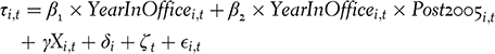 (4.4)
(4.4)
 (4.5)
(4.5)
The subscripts
 and
and
 denote prefecture and year, respectively.
 represents SO2 regulatory stringency, proxied by the SO2 removal ratio and the NO2-to-SO2 concentrations ratio.
 is a vector of industrial firm characteristics.
 denotes prefecture fixed effects, which capture time-invariant characteristics within a prefecture that may influence the SO2 removal ratio.
 represents year fixed effects, which account for year-to-year unobserved factors that influence changes in the average
 .
.
 should absorb the effects of national changes in SO2 pollution levy rate and top-down regulation campaigns.
 represents the standard idiosyncratic disturbance term. I cluster standard errors at the prefecture level to adjust for serial correlation over time in a prefecture.
The coefficients of interest are
 and
and
 , which measure the response of environmental regulation to the effect of tenure when the prefecture was under nonbinding and binding SO2 reduction targets, respectively. The specification in Eqs. (4.4) and (4.5) allows for the identification of the tenure effect under the 10th FYP (2001–5) separately from the tenure effect under the 11th FYP (2006–10).
Results in Table 4.2 suggest that during a given tenure, prefectures with high reduction targets experienced an average annual decrease in 0.28 unit of SO2 removed per 1 unit of SO2 generated under the 10th FYP (2001–5). In contrast, the average decrease in SO2 removal ratio from year to year had reduced from 0.28 to
 – suggesting Weberian-esque regulation – under the 11th FYP (2006–10). In other words, there were progressively less SO2 abated vis-à-vis produced year after year under the 10th FYP, as compared to the 11th FYP. However, the same significant effects are not observed, based on the current measurements, when the treated observations are analyzed as a whole.
Table 4.2 Relationship between political tenure and SO2 regulatory stringency under the 10th FYP (2001–5) and the 11th FYP (2006–10)
| SO2 regulatory stringency | ||
|---|---|---|
| Year in office | −0.28***(0.06) | −0.27***(0.08) |
| (Year in office)2 | −0.00(0.01) | |
Year in office
 post-2005
 | 0.23***(0.07) | 0.22*(0.09) |
(Year in office)2
 post-2005
 | 0.00(0.01) | |
| Controls | Y | Y |
| Fixed effects | Y | Y |
| Num. obs. | 238 | 238 |
| Num. clusters | 32 | 32 |
Notes: Standard errors are clustered at the prefecture level and appear in parentheses; figures are rounded to the second decimal.
* indicates significance at the 10% level.
** indicates significance at the 5% level.
*** indicates significance at the 1% level.
Due to the availability of annual satellite-based SO2 and NO2 statistics (2005–present), I regress year in office on SO2 regulatory stringency under the 11th FYP (2006–10). The results in Table 4.3 based on both officially reported data and satellite-derived statistics would suggest that the binding status of SO2 reduction targets introduced under the 11th FYP created incentives for career-minded local leaders to ensure consistent implementation of SO2 regulation.Footnote 29
Table 4.3 Relationship between political tenure and SO2 regulatory stringency under the 11th FYP (2006–10)
| SO2 regulatory stringency | ||||
|---|---|---|---|---|
| SO2 removal ratio (official) |
 (satellite)
 | |||
| Year in office | −0.07(0.04) | −0.05(0.05) | −1.59(6.10) | −4.77(10.33) |
| (Year in office)2 | −0.00(0.01) | 0.77(1.62) | ||
| Controls | Y | Y | Y | Y |
| Fixed effects | Y | Y | Y | Y |
| Num. obs. | 144 | 144 | 143 | 143 |
| Num. clusters | 32 | 32 | 31 | 31 |
Note: Clustered standard errors appear in parentheses.
* indicates significance at the 10% level.
** indicates significance at the 5% level.
*** indicates significance at the 1% level.
4.5 Conclusion
SO2 control is a case where all three scope conditions of the theory are satisfied. Since SO2 emissions management entails a low level of ambiguity, regulatory efforts translate well into regulatory effectiveness. The official and satellite-derived statistics reflect the level of regulatory effectiveness, and, by extension, regulatory efforts in regulating SO2 emissions. The empirical evidence shows that top prefectural leaders whose prefectures received high reduction targets were incentivized to induce an incremental, steady decrease in regulatory stringency under the 10th FYP and a relatively consistent implementation under the 11th FYP (Figure 4.2); the more regularized pattern under the 11th FYP is observed based on evidence from both official and satellite-based statistics.
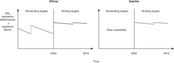
Figure 4.2 Local political regulation waves before and after the imposition of binding reduction targets for SO2 emissions, official statistics versus satellite-derived statistics
The absence of ambiguity in the emissions sources and the goal and means to control SO2 boded well for the alignment of the preferences of central leaders with the efforts and the efficacy of those efforts of local leaders, especially when incentives were strong. Will the shift from a political pollution wave to a political environmental protection wave still hold and be observable when the air pollutant has more diverse sources, promising more ambiguity and therefore a greater challenge for effective management? In the following chapter, I explore that question by extending the analytical framework of the political regulation wave theory to the case of PM2.5 pollution.


 Open access