
1.1 Introduction
Geopressure is the pressure beneath the surface of the earth. It is also known as the formation pressure. This could be lower than, equal to, or higher than the normal or hydrostatic pressure for a given depth. Hydrostatic or normal pressure is the force exerted per unit area by a column of freshwater from the earth’s surface (e.g., sea level) to a given depth. Geopressures lower than the hydrostatic pressures are known as underpressures or subpressures, and they occur in areas where fluids have been drained, such as a depleted hydrocarbon reservoir. Geopressures higher than hydrostatic pressures are known as overpressured, and they occur worldwide in formations where fluids are trapped within sediments due to many geologic conditions and support the overlying load. Overpressured formations are also known as formations with abnormally high pore pressure. The lithostatic (or overburden) pressure at a given depth is due to the combined weight of the overlying rock and fluids. The fracture pressure is the pressure that causes the formation rock to crack. Figure 1.1 shows these concepts in graphical terms.

Figure 1.1 Pressure versus depth plot showing geopressure regimes.
If the overlying fluid is composed of hydrocarbon as well as water (brine), the pressure versus depth plot will look like that shown in Figure 1.2.

Figure 1.2 Pressure versus depth plot showing buoyancy effect due to hydrocarbons.
The slope changes in the plot are due to density differences between brine, oil, and gas. The overpressure phenomenon is well known throughout the world. Among other things, the magnitude and distribution of overpressure in sedimentary basins have been known to critically impact the evolution of hydrocarbon provinces, control the migration of fluids within a basin, and affect the processes that are used to mine the subsurface resources, such as oil and gas. The most discussed and well-known cause of overpressure is the rapid burial of low-permeability water-filled sediments (e.g., clay) at a rate that does not allow the fluid to escape fast enough to maintain hydrostatic equilibrium upon further burial. Thus, further burial causes geopressure to rise even more. This is known as compaction disequilibrium. This is the leading cause of overpressure in most of the Tertiary clastic basins of the world, such as the Gulf of Mexico. This and many other mechanisms of overpressure are discussed in detail in Chapter 3.
1.2 Basic Concepts
1.2.1 Units and Dimensions
Before we proceed, a word on units and dimensions is in order. All quantities in physics must either be dimensionless or have dimensions. All units can be expressed in terms of mass [M], length [L], and time [T]. In equations, the units must be consistent; there is no need for conversion factors. However, care is needed for quantities, such as pressure. It is force per unit area. The dimension of force is [ML−1T−2]; but if the unit of length is feet and the unit of pressure is pounds per square inch, or psi (as is commonly used in the US drilling community), a conversion factor is required, since these are inconsistent mixed units. In SI units, such conversion factors are not needed because all the units are consistent. The lack of inconsistency of units using the American system is known to have created a massive headache between the two drilling communities – those who use the SI units (some communities in Europe, for example) and those who do not use SI units. We shall discuss this further in this chapter in the context of pore pressure measurements.
As mentioned, pore pressure has the dimension of force per unit area. In the SI system, the unit of pressure is pascal (Pa), and in the British system, the unit is pounds per square inch (psi). We note that 1 Pa = 1.4504 × 10⁻⁴ psi. This is a rather small unit, and for most practical applications, it is customary to use either kilopascal (KPa) or megapascal (MPa). Drillers, engineers, and well loggers still use the British system, while the academicians prefer the SI system. Therefore, a fluency in both type of units is a must. We will be using the mixed system throughout the book. However, whenever possible, we will provide the SI or British system equivalents.
1.2.2 Hydrostatic Pressure
Sedimentary rocks in formations are composed of solid material and fluids in the porous network. Hydrostatic or normal pressure,  , is the pressure caused by the weight of a column of fluid and is given by
 (1.1)
(1.1)
where z is the column height of the fluid,  is the density of the fluid, g is the acceleration due to gravity, and
  denotes the pressure due to the atmosphere. The size and shape of the fluid column have no effect on hydrostatic pressure. The approximation on the right-hand side of equation (1.1) assumes that
  is constant and z is the depth below sea level or the land surface. Hydrostatic pore pressure increases with depth; the gradient at a given depth is dictated by the fluid density at that depth. This is because the water or brine density is not constant. Water tends to expand with rising temperature but contracts with rising pressure. As we shall see later, between the two processes in the subsurface (i.e., increase in temperature and pressure), thermal expansion with increasing depth is greater than the mechanical compression. There are other factors that affect the water density, such as dissolved salt – the solubility of salt also increases with depth. Subsurface brines are more saline than the ocean water. This increase in total dissolved salt increases the density of water. The net effect is that the water (brine) density is a complex function of temperature, pressure, and total dissolved solids. If a subsurface formation is in the hydrostatic condition, it implies that there is an interconnected and open pore system from the earth’s surface to the depth of measurement. To summarize, the fluid density depends on various factors, such as fluid type (oil, water, or gas), concentration of dissolved solids (i.e., salts and other minerals), and temperature and pressure of the fluid and gases dissolved in the fluid column. In Appendix A we provide some practical empirical relationships for physical properties of brine, gas, and oil needed for quantitative analysis of geopressure.
We strongly recommend that those who wish to pursue quantitative evaluation of geopressure use those equations for density and velocity of brine, gas, and oil (“dead” and “live”) in a computer code. This will enable them to evaluate the true hydrostatic pressure as well as the pressure due to gas and oil columns of various heights. Here “dead” oil designates oil without any dissolved gas, whereas “live” oil means it contains dissolved gas.
What would a pressure versus depth plot such as the one in Figure 1.1 look like for a reservoir rock containing gas, oil, and water? An example is given in Figure 1.2 for the case of a reservoir filled with gas, oil, and water (brine). The slope changes are due to the density contrast between different kinds of fluids (gas, oil, brine), as discussed earlier. This kind of plot is very useful for determining the height of a hydrocarbon column in a reservoir. The discrete data points show actual measurements of pore pressure in a reservoir. Typically, not many measurements are carried out, as measurements are expensive in a real petroleum well; petroleum engineers make these discrete measurements and then look for slope changes to determine gas–oil and oil–water contacts, which yield the hydrocarbon column height. Eventually, seismic data are used along with geologic structure maps of a prospect to map these contacts in 3D. Volumetric calculations resulting from these measurements, along with uncertainty estimates, are used to determine the ultimate value of the asset.
1.2.3 Head
We introduce some terminology commonly used in fluid dynamics and relevant to geopressure. In the subsurface, fluids always move, although the speed at which they move is small in the human timescale. It is not so in the geologic timescale. The definitions that we gave in Section 1.2.2 are for fluids in the static condition. In fluid mechanics literature, the word head is commonly used. Head refers to a vertical dimension and has the dimension of length [L]. There are various types of heads.
A pressure head (also termed as static pressure head or static head) is the vertical elevation of the free surface of water above the point of interest. It is given by
 (1.2)
(1.2)
where
 is the pressure head (length, typically in units of m)
P is the fluid pressure (force per unit area, typically in units of Pa)
-
is the specific weight (force per unit volume, typically in units of Newton/m3)
-
is the density of the fluid (mass per unit volume, typically in kg/m3)


The term hydraulic head or piezometric head is used to specify a specific measurement of liquid pressure above a datum. It is composed of three terms: velocity head ( ), elevation head (
 ), and pressure head (
 ). The following is referred to as the head equation:
 (1.3)
(1.3)
Here C is a constant for the system (referred to as the total head) that appears in the context of the Bernoulli equation for incompressible fluids in hydrodynamics, which states that an increase in fluid speed occurs simultaneously with a decrease in pressure (Reference StreeterStreeter, 1966). The velocity head (also referred to as kinetic head) is the head due to the energy of movement of the water. (In subsurface flow through porous rocks, this is negligible.) The elevation head is the elevation of the point of interest above a datum, usually sea level or the land surface.
1.3 Pore Pressure Gradient
A gradient is the first derivative of a physical quantity. The pressure gradient, dp/dz, is the true gradient of pore pressure, p, versus depth at a given point z. It shows change of pore pressure in a small scale. It is the rate at which pressure varies along a uniform column of fluid due to the fluid’s own weight. Thus, a change in gradient implies a change in fluid density. Local gradients are most useful when working with the absolute pressure. However, the drilling community uses a term called pore pressure gradient to denote the density of fluid. It is the ratio of the pore pressure (p at a depth z) to the depth z. This is usually expressed in pounds per square inch per foot (abbreviated by psi/ft) in the British system of units and MPa/m in the SI system. It is clear that this gradient is datum dependent. Furthermore, pore pressure gradient is not the true gradient of p as a geoscientist or an engineer would define. It is simply pressure/depth. The conversion between fluid density and fluid pressure gradient is
Thus, the fluid density, can be defined as
The drilling community uses a term called equivalent mud weight (EMW) to denote the density of fluid (mud) required to drill a well. It is expressed in pounds per gallon, abbreviated as ppg. A conversion factor for equivalent mud weights is
Weight in itself is not a gradient. If we relate weight to a volume, however, we have density, and density does convert to a gradient. When we refer to mud weights as 10 pounds, we mean the mud density is 10.0 lb/gal or ppg. This is a density. (In this nomenclature, pure water density would be 8.344 ppg.) Reference FertlFertl (1976) suggested the following relation for hydrostatic pressure in psi, as is commonly used in drilling operations:
 (1.7)
(1.7)
where  is the vertical height of fluid column in feet, Mw is fluid density for mud weight expressed in lb/gal (or ppg) or pounds per cubic feet (lb/ft3), and C is a conversion constant equal to 0.0519 if Mw is expressed in pounds per US gallon and 0.00695 if Mw is expressed in lb/ft3. The conversion factor 0.0519 (inverse of 19.250) is derived from dimensional analysis as follows:
 (1.8)
(1.8)
It would be more accurate to divide a value in lb/gal by 19.25 than to multiply that value by 0.052. The magnitude of the error caused by multiplying by 0.052 is approximately 0.1 percent. Let us take an example: for a column of freshwater of 8.33 pounds per gallon (lb/US gal or ppg) standing still hydrostatically in a 21,000 ft vertically cased wellbore from top to bottom (vertical hole), the pressure gradient would be
and the hydrostatic bottom hole pressure (BHP) is then BHP = true vertical depth × pressure gradient = 21,000 (ft) × 0.43273 (psi/ft) = 9087 psi. However, the formation fluid pressure (pore pressure) is usually much greater than the pressure due to a column of freshwater, and it can be as much as 19 or 20 ppg. For an onshore vertical wellbore with an exposed open hole interval at 21,000 ft with a pore pressure gradient of 19 ppg (or 19 × 0.0519 (psi/ft)), the BHP would be BHP = pressure gradient × true vertical depth = 19.0 × 0.0519 (psi/ft) × 21,000 (ft) = 20,708 psi. (It would be 20,727 psi if we replace 0.0519 by 1/19.25. ) The calculation of a bottom hole pressure and the pressure induced by a static column of fluid (drilling mud) are the most important and basic calculations in the petroleum industry. In summary, pore pressure gradient is a dimensional term used by drilling engineers and mud engineers during the design of drilling programs for drilling (constructing) of oil and gas wells into the earth. In Table 1.1 we give some useful conversion factors.
Table 1.1 Units and conversions
| Psi | = 0.070307 kg. force/cm2 |
| Atm | = 1.033 kg force/ cm2 |
| Atm | = 14.6959 psi |
| Psi | = 0.006895 MPa |
| Psi/ft | = 2.31g/cm3 |
| = 1 4 4 lb / ft3 | |
| = 19.25 lb/gallons or ppg | |
| 1 Pa = 1N/m2 = 1.4504 x 10⁻⁴ psi | |
| 1 Mpa = 106 Pa = 145.0378 psi | |
| 1 Mpa = 10 bars | |
| 1 N = 1 kg. m/s2 | |
| 1 kbar = 100 MPa | |
| 1 psi / ft. = 2.31 g/cm3 | |

| |
In the Gulf Coast of the United States, a fluid pressure gradient of 0.465 psi/ft is considered to be normal or hydrostatic; it corresponds to a salt concentration of 80,000 ppm and a temperature of 77°F. However, the hydrostatic pressure gradient is variable depending upon the temperature, pressure, and salinity, as noted earlier. An increase in salt concentration at a given temperature and pressure would increase the hydrostatic gradient. Dissolved gas in water, for example, methane, also affects the density of water – it lowers the density – and hence the hydrostatic gradient will be lower. We note that the solubility of methane in water is a function of salt concentration at a given temperature and pressure – it increases with increasing salt concentration. Thus, dissolved gases would cause the hydrostatic gradient to be lower. In the vicinity of salt domes, salt concentration could be markedly higher, leading to a higher hydrostatic gradient. In Table 1.2 we show typical values for density and pressure gradients for oil, brine, and some drilling fluids. In Table 1.3 we show typical hydrostatic pressure gradients for several areas of active drilling.
Table 1.2 Fluid densities and corresponding pressure gradients
| Fluid | Total solids | Density | Fluid pressure gradient | |
|---|---|---|---|---|
| (ppm) | (g/ml) | (psi/ft) | (kPa/m) | |
| Freshwater | 0 | 1.0 | 0.433 | 9.8 |
| Brine | 28,000 | 1.02 | 0.441 | 10.0 |
| 55,000 | 1.04 | 0.450 | 10.2 | |
| 84,000 | 1.06 | 0.459 | 10.4 | |
| 113,000 | 1.08 | 0.467 | 10.6 | |
| 144,000 | 1.10 | 0.476 | 10.8 | |
| 176,000 | 1.12 | 0.485 | 11.0 | |
| 210,000 | 1.14 | 0.493 | 11.2 | |
| Oil | API° (60°F) | |||
| 70.6 | 0.70 | 0.303 | 6.90 | |
| 45.40 | 0.80 | 0.346 | 7.80 | |
| 25.70 | 0.90 | 0.390 | 8.80 | |
| 10.00 | 1.00 | 0.433 | 9.80 | |
| Drilling mud | lb/gal or ppg | |||
| 8.35 | 1.00 | 0.433 | 9.80 | |
| 10.02 | 1.20 | 0.520 | 11.8 | |
| 11.69 | 1.40 | 0.607 | 13.70 | |
| 13.36 | 1.60 | 0.693 | 15.70 | |
| 15.03 | 1.80 | 0.780 | 17.70 | |
| 16.70 | 2.00 | 0.867 | 19.60 | |
| 18.37 | 2.20 | 0.953 | 21.60 | |
| 20.04 | 2.40 | 1.040 | 23.50 | |
| 21.71 | 2.60 | 1.126 | 25.50 | |
| 23.38 | 2.80 | 1.213 | 27.50 | |
| 25.05 | 3.00 | 1.300 | 29.40 |
Note: Pressure gradients are related to the specific gravity ( ) rather than the density (
 ), where
 , g = 9.81 m/s2.
Table 1.3 Normal pore pressure gradients for several areas
| Area | Pressure gradient (psi/ft) | Pressure gradient (g/cc) |
|---|---|---|
| West Texas | 0.433 | 1.000 |
| Gulf of Mexico (coastline) | 0.465 | 1.074 |
| North Sea | 0.452 | 1.044 |
| Malaysia | 0.442 | 1.021 |
| Mackenzie Delta | 0.442 | 1.021 |
| West Africa | 0.442 | 1.021 |
| Anadarko Basin | 0.433 | 1.000 |
| Rocky Mountains | 0.436 | 1.007 |
| California | 0.436 | 1.014 |
It is clear from these discussions that hydrostatic (or normal) pressure for a static water column of height z is equivalent to a water-saturated porous medium such as clean sandstone of the same height with the assumption that the sandstone consists of interconnected pores. Formation pressure (or geopressure) that differs from hydrostatic pressure is defined as abnormal pressure. Formation pressure (or geopressure) exceeding hydrostatic pressure is defined as overpressure, whereas formation pressure lower than hydrostatic is defined as subpressure. Therefore, we emphasize that before embarking on any computation involving determination of subsurface pore pressure, we must establish a proper baseline – deciding on the “accurate” hydrostatic pressure gradient with as much accuracy as possible.
1.4 Overburden Stress
The overburden or lithostatic stress,  , at any depth,
  , is the stress that results from the combined vertical weight of the rock matrix and the fluids in the pore space overlying the formation of interest as well as the weight of the static water column, if in an offshore environment, and the atmospheric air pressure. This can be expressed as

where  is the pressure due to the atmospheric air column (typically 14.5 psi or 1 bar),
  is the bulk density,
  is the sea water density (both depend on depth),
  is depth to the ocean bottom, and g is the acceleration due to gravity. The bulk density of a fluid-saturated rock is given by
 (1.11)
where ϕ is the fractional porosity (the void space in the rock),  is the pore fluid density, and
  is the density of the matrix (grain density). It should be noted that the overburden stress computation in the context of drilling wells should always account for the air gap or the atmospheric pressure. Although this is small, it could be significant while dealing with overburden stress in shallow formations, such as pressured aquifer sands or methane hydrates, as discussed later. Overburden stress is depth dependent and increases with depth in a nonlinear fashion. In some of the older literature on geopressure, a default value of 1.0 psi/ft for overburden stress gradient (overburden stress divided by depth) has been recommended for the “average” Tertiary deposits off the Texas–Louisiana coast. This corresponds to a force exerted by a formation with an average bulk density of 2.31 g/cm3. However, this is not true in reality, where we always deal with rocks of variable bulk densities. At shallower depths, the overburden gradient would be less than 1.0 psi/ft, while at deeper depths, it could be larger than 1.0 psi/ft. In Figure 1.3 we show typical overburden gradients from selected basins.

Figure 1.3 Typical overburden stress gradients versus depth in psi/ft and ppg.
1.5 Effective Vertical Stress and Terzaghi’s Law
When a rock is subjected to an external stress, it is opposed by the fluid pressure of pores in the rock. This is due to Newton’s law of classical mechanics. More explicitly, if  is the formation or pore fluid pressure at a depth where the vertical component of the total stress (namely, the vertical overburden stress) on it is
  , then the vertical effective stress σ is defined as (see Figure 1.4)

Figure 1.4 Subsurface pressure environment and some commonly used definitions.
 (1.12)
This is known as the Terzaghi’s principle or law (Reference TerzaghiTerzaghi, 1923). This principle was invoked to describe the consolidation of soil in the context of geotechnical engineering (soil consolidation) (see Chapter 2). Compaction is due to the vertical effective stress – it is the stress that is transmitted through the solid framework. This (vertical effective stress) is a very important parameter to describe geopressure phenomenon quantitatively, especially when geophysical methods such as seismic or sonic logs are used to quantify geopressure. A relationship between velocity and overpressure is intuitively expected, since acoustic velocity and vertical effective stress are related closely. This will be discussed in Chapter 3. We note that Terzaghi’s Law is only an approximation because the vertical component of the total stress  does not remain constant in a sedimentary basin that is actively developing and accumulating sediment, nor does it remain strictly constant during compaction of sedimentary rocks (see Chapter 2). It has several other assumptions as well: The soil is isotropic and homogenous; the solid particles and fluids are incompressible; the fluid flow occurs in one dimension only (vertical direction); the strains in the soil are very small (linearized strain model); Darcy’s law for fluid flow is valid for all pressures (linearized fluid flow model); the permeability remains constant throughout the process; and lastly, compaction process is independent of time. While some of the assumptions are reasonable and borne out by experiments, the remainder of the assumptions such as the linearity of strain, one-directional flow model as well as the time-independence of the compaction process (relationship between porosity and vertical effective stress) may be questioned.
Subsequent literature such as Reference Hornby, Schwartz and HudsonHornby et al. (1994, and references therein) as well as Reference Sarker and BatzleSarker and Batzle (2008, and references therein) suggested using the Biot model for the effective stress as given below, instead of Terzaghi’s Law (see Chapter 2):
 (1. 13)
where  is termed as Biot’s consolidation coefficient and its value lies between 0 and 1. Further, it was mentioned that this coefficient could depend on the lithology also. Reference Sarker and BatzleSarker and Batzle (2008) and Reference Hornby, Schwartz and HudsonHornby et al. (1994) suggested that
  is close or equal to unity for near-surface sediments such as soil and clay – the subject of measurements by Reference TerzaghiTerzaghi (1923) but for consolidated rocks, it could be less than unity and its value is ~ 0.90 to 0.93 as determined by laboratory measurements using ultrasonic waves (Reference Hornby, Schwartz and HudsonHornby et al., 1994). Suffice it to say at this point that the uncertainty regarding
  is related to three major factors: (1) what are the “assumed” physical processes by which unconsolidated sediments morph into rocks under gravitational loading and many chemical effects? (2) How are the measurements conducted, namely, under static or dynamic conditions? and (3) what kind of rock types are considered in the measurements? It must be noted that there is no direct way to measure
  ; it is derived indirectly from measurements of physical quantities which are related to the effective stress such as pore pressure and velocity. We note that Biot’s consolidation coefficient plays an important role in building geomechanical models (see Chapter 12). In our discussions in this book we shall continue to use
  = 1 and the original version of the Terzaghi’s Law as given in equation (1.12) unless otherwise stated. In Chapter 2 we will show a simple derivation of Terzaghi’s Law based on Archimedes’ principle for solid particles suspended in a fluid.
There are many field evidences of Terzaghi’s Law. It is the reason why the surface over oil fields subsides after hydrocarbon or other fluids are produced (Reference KuglerKugler, 1933; Reference GabryschGabrysch, 1967; Reference MayugaMayuga, 1970). In these examples (and there are many examples, such as the subsidence of the Ekofisk oil field in the Norwegian Sector of the North Sea and various offshore fields in the Gulf of Mexico and Louisiana, USA), the extraction of liquids led to a reduction in pore pressure, an increase in the effective stress ( ), and hence further compaction and subsequent subsidence of the reservoirs. In these cases, the reservoir pressure is less than the normal or hydrostatic pressure and gas and water are injected to counter the subsidence. In the case of Ekofisk Field, the drop in pore pressure was shown to be balanced by an increase of the effective stress in accordance with the Terzaghi’s Law (Reference Chapman, Fertl, Chapman and HotzChapman, 1994a). Such effects can be monitored by 4D-seismic techniques (see Chapter 12).
1.6 Formation Pressure
As defined earlier, formation pressure is the pressure acting on the fluid contained in the pore spaces of sediments or rocks. Figure 1.1 illustrates a typical geopressure versus depth profile. The geopressure regime could be loosely classified in three zones: Subnormal or subpressure where pore pressure is below hydrostatic pressure; hydrostatic or normal pressure; and overpressure where the pore fluid pressure is higher than the hydrostatic pressure. The transition from hydrostatic to overpressure may be fairly well-defined as in the Miocene sections of the Texas–Louisiana Gulf Coast, or gradual as in the case of deepwater Pliocene and Pleistocene sections of the many Tertiary Clastic provinces in the world. The depths at which these transitions occur and the shape of the transition zone depend mostly on the permeability (it controls the fluid flow out of the sediments) and the rate of deposition of the sediments (it provides the source of the fluid in the sediments). Typically when the outflow of fluids (brine) is less than the inflow, the system is overpressured as the fluid begins to support the load. This mostly dictates the magnitude and the distribution of pore pressure. The extent of the transition zone can vary from a few hundred feet to many thousands of feet. Although there is no universally accepted scale expressing the degree of geopressuring, the nomenclature introduced by Reference DuttaDutta (1987a, Table 1, p. 5) is commonly accepted. This is reproduced in Table 1.4.


An important concept seen in Figure 1.4 is that pore pressure typically does not reach overburden stress. As pore pressure approaches overburden stress (actually, the least principal confining stress which is usually less than the overburden stress as discussed in Chapter 2), fractures in the rock open and release fluids and pressures. The pressure at which this happens is termed as the “fracture pressure.” Thus, every rock has a characteristic limit defined as the seal limit in Figure 1.4. Fracture pressure at a given depth divided by the depth is known as the fracture gradient at that depth. There are three important quantities that the drilling community is mostly concerned with prior to drilling a well. These are: pore pressure gradient, fracture gradient and overburden gradient. All gradients are typically converted to EMW and the drilling plan deals with obtaining these quantities for the entire well.
Variation in the effective stress is also shown in Figure 1.4. It is the difference between overburden or lithostatic stress and pore pressure, i.e., essentially the amount of overburden stress that is supported by the porous network of rock grains as is allowed by the Reference TerzaghiTerzaghi (1923) principle. If we assume that the pore fluid consists of brine with the density of 1.07 gm/cc (equivalent to a pressure gradient of 0.465 psi/ft), the normal or hydrostatic fluid pressure (in psi) will be given by
 (1.14)
In this case, the effective stress (σ) will be given by
 (1.15)
if we assume an overburden stress gradient of 1.0 psi/ft (i.e., equivalent to an assumed average and constant bulk density of 2.31 gm/cc). Reference Hubbert and RubeyHubbert and Rubey (1959) defined a quantity, λ, as the ratio between the formation pressure and the vertical overburden stress given by
Then,
Some authors (e.g., Reference FertlFertl, 1976) used λ = 0.9 as an estimate of the upper limit of pore pressure in regressive sequences such as in the Tertiary rocks in the Gulf of Mexico, USA. They suggested that beyond this limit (seal limit) hydraulic fracture of the sedimentary rocks was a distinct possibility. Some practitioners use this as a measure of fracture pressure. However, the subject of subsurface fracturing due to overpressure (a natural cause) is more complex and it depends on many other factors besides pore pressure, such as lithology and tectonic stress and its orientation (Reference ZobackZoback, 2007). We shall discuss this in more detail in Chapter 2. Reference Hubbert and RubeyHubbert and Rubey (1959) also introduced a useful concept – equilibrium depth  . This is defined as the depth where the effective stress is equal to what it would be at a shallower depth, had the rocks compacted normally. Reference Swarbrick, Osborne and YardleySwarbrick et al. (2002) introduced the term fluid retention depth (FRD) – it is the depth at which pore pressure begins to get higher than the normal pressure; it is also the depth where the effective stress (σ) reaches its maximum value (see Figure 1.4). We note that as pore pressure increases, so does the drilling time, cost and risk.
Overpressure implies low effective stress – lower than the effective stress for hydrostatic pressure conditions. Thus, it is maximum at the depth where the departure from hydrostatic to overpressure occurs. Drilling experiences have shown that the lowering of the effective stress in the overpressured zone is not “sharp” – it is typically preceded by a zone of almost constant effective stress. This has to do with various competing pressure mechanisms for generating geopressure as we shall see later in Chapter 3. The variables required for predicting and assigning prospect risks for prospectivity of hydrocarbons are (see Figure 1.4)
– the depth of the top of the overpressured zone,
– the depth of the top of the “hard overpressured” zone,
– the shape of the transition zone, and
– seal failure limit (the pressure needed to induce hydraulic fracturing of the “seal or cap rocks”).
Let us consider the geometry of a brine-filled reservoir as shown in Figure 1.5. The reservoir is truncated at a fault and we assume that the fault is a sealing fault, namely, it does not allow any fluid to flow across the fault. In the absence of fluid flow, the difference in pore pressure between points A and B is simply the weight of the fluid in the vertical reservoir column (Figure 1.5a). If this fluid is water, pore pressure at any elevation in the reservoir will follow a hydrostatic slope as shown in Figure 1.5b. If the reservoir is overpressured and filled with brine, pore pressure will track a line parallel to the normal hydrostatic pressure curve for brine, which means that overpressure at each depth is the same as shown in Figure 1.2. This is important because it means that overpressure in a continuous reservoir unit must be constant throughout the water-bearing portion of the reservoir. This situation occurs because the permeability of the reservoir sand is much higher than that of the encasing impermeable rock (shale). In Figure 1.5, the pore pressure at the updip location (B) is related to the pore pressure in the downdip direction (A) by

Figure 1.5 (a) Pore pressure profile of a reservoir sand with structure embedded in an overpressured shale. (b) For an overpressured sand filled with brine, the pore pressure tracks a line parallel to the normal hydrostatic pressure curve for brine.

In Figure 1.6 we show on the left a schematic geologic cross section of a hydraulically connected reservoir filled with gas of column height hg, oil of column height ho and brine. The right figure shows pore pressure elevated by hydrocarbon columns. This pressure profile is due to the buoyancy effect of the fluids. Typical values of fluid densities are 1.05 g/cm3 for water (brine), 0.7 g/cm3 for oil, and 0.23 g/cm3 for gas as indicated by the slope changes of the pressure profiles on the right. It is clear from equation (1.18) and the buoyancy effect of hydrocarbons that at the crest of the structure, the pore pressure gradient would be larger than the case when the reservoir was brine saturated. This increases the possibility of the caprock failure. It is for this reason, drillers usually do not spud a well directly at the crest of a structure.

Figure 1.6 Schematic of a reservoir saturated with gas, oil, and water (left) and pore pressure elevated by oil and gas columns and density contrast between water, oil, and gas in a reservoir. Typical density contrasts are given in the figure on the right. (left) A hypothetical geologic cross section. (right) Pore pressure elevated by hydrocarbon columns in a hydraulically connected formation as depicted in cross section on the left.
1.6.1 Subpressure
Subpressure formations are those in which the pore pressure is below the hydrostatic pressure. Such pressure conditions are known to exist in many depleted oil reservoirs, in areas with withdrawal of ground water and attendant local subsidence and in lenticular reservoirs closely associated with shales in areas that have undergone erosion. Since pore pressure gradient is datum dependent, the local topography plays a significant role. Pressure gradients can be either lower or higher than the hydrostatic pressure gradient. In Figures 1.7a–c, we show three possibilities where the outcrop elevation and the well site elevation determine the pore pressure gradient as measured in that well bore. Figure 1.7a shows the normal pressure situation where the well elevation is the same as the outcrop elevation. The pressure gradient at the wellbore is 0.465 psi/ft (0.0105 MPa/m). Figure 1.7b shows the abnormally high pore pressure situation where the well elevation is lower than the outcrop elevation. The pore pressure at the wellbore is 0.465 psi/ft × 13,000 ft = 6045 psi (41.6787 MPa), leading to a pressure gradient of 6045 psi/10,000 ft = 0.6045 psi/ft (0.01360 MPa/m). Figure 1.7c shows a situation where abnormally low or subnormal pressure occurs where the well elevation is higher than the outcrop elevation. In this case, the pore pressure at the well site is 0.465 psi/ft × 7000 ft = 3255 psi (22.4483 MPa) leading to a pressure gradient of 3255/10,000 ft = 0.3255 psi/ft (0.007323 MPa/m) which is lower than the normal pressure gradient. We note that subpressures are relatively uncommon except for depleted reservoirs. Proximity to a mountain range is also a feature that relate to subpressures – it provides a sink through which water is abstracted from the basins.
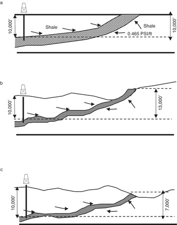
Figure 1.7 Effect of datum on pore pressure gradient. (a) Well elevation is the same as that of the outcrop elevation. (b) Well elevation is lower than the outcrop elevation leading to an abnormally high-pressure gradient. (c) Well elevation is higher than the outcrop elevation, leading to an abnormally low-pressure gradient.
1.6.2 Fracture Pressure
In oil field terminology, fracture pressure is the pressure that causes a formation to fracture and the circulating fluids to be lost. Normally it is expressed as the fracture gradient or the fracture pressure divided by the depth. In this way, it determines the maximum mud weight that can be used to drill a well bore at a given depth. Hence it is an important parameter for mud weight design in both the drilling planning stage and in the drilling stage. If the mud weight is higher than the fracture gradient of the formation the well bore will undergo tensile failure, causing losses of drilling mud or even lost circulation. In practice, fracture pressure is measured from various types of leak-off tests (LOT). A leak-off test is performed to estimate the maximum amount of pressure or fluid density that the test depth can hold before leakage and formation fracture may occur. This measurement is usually made at the casing points. There are several approaches to calculate fracture gradient. We shall discuss this in details later (Chapters 2 and 4).
1.6.3 Equivalent Circulation Density (ECD)
This is an important concept in drilling. Hydrostatic weight of the mud is intended to balance the formation pressure under “static” condition. During drilling, mud pumps are turned on and the situation is no longer static. In this case, the borehole geometry introduces pressure loss based on drag on the fluid as it passes through the various components of the fluid flow path during drilling such as standpipe, drillstring components, open hole, and casing. The mud pumps supply the pressure that forces drilling mud down the drill string to the bottom of the hole and up again to the surface. As the drilling mud exits the bit nozzles, the mud has to flow through the annular space between the drill string and the borehole wall. Contact is made between the drilling mud and the borehole wall as the drilling mud flows upward to the surface. This contact creates “drag” as the result of friction and the drilling mud loses some of the pressure supplied by the pump in order to overcome this frictional drag. This pressure loss is absorbed by the formation. Equivalent circulating density (ECD) is the effective density that combines current mud density and annular pressure drop. Thus, ECD in ppg = (annular pressure loss in psi) ÷ 0.052 ÷ true vertical depth (TVD) in ft + (current mud weight in ppg). This is why the ECD is always greater than the mud density under static condition. The greater the vertical distance through which the drilling mud has to travel until it reaches the surface, the higher are the pressure drop and ECD. Note that ECD is a function of the true vertical depth and not the measured depth. Measured depth includes the horizontal section in deviated wells but ECD only depends on the true “vertical” depth. Acquired solids (cuttings), the type of mud and its temperature also affect ECD.
1.7 Casing Design
Both pore pressure and fracture pressure dictate the casing design in drilling. A casing is a large heavy steel pipe which is lowered into the well. Generally, a casing is subjected to various physical and chemically related loads during its lifetime. Its purpose is to prevent collapse of the borehole while drilling, hydraulically isolate the wellbore fluids from formations and formation fluid, minimize damage of both the subsurface environment from the drilling process and from extreme subsurface environment, provide a high strength flow conduit for the drilling fluid, and provide safe control of formation pressure. If the casing is properly cemented it can also help to isolate communications between different perforated formation levels. Selection of the number of casing string and their respective setting depths generally is based on a consideration of the pore pressure gradients and fracture gradients of the drilling area. In Figure 1.8, we show a typical casing design for a hydrocarbon well.

Figure 1.8 Typical casing strings used in the hydrocarbon industry.
A casing string consists of (1) surface casing, (2) intermediate casing, (3) liners, and (4) production casing. The main purpose of the surface casing is to prevent the shallow water region from contamination, the structural support for weak soil areas near the subsurface, and also protect the casing strings inside. Again, this can prevent blowout and can close the surface casing in the event of a kick or explosion. When drilling deeper through weak zones like salt sections and abnormally pressurized formations, these unstable sections need more pipe sections, in the form of intermediate casings between the surface casing and the final casing. When abnormal pore pressures are present below the surface casing, intermediate casings are needed to protect the formation. The liner is a casing string that does not extend to the surface. It is suspended from the bottom of the next large casing string. The principal advantage of a liner is its lower cost. It serves as a low cost intermediate casing. This casing string provides protection for the environment in the event of a failure during production. Generally, there are two types of wells. The first are exploration wells that are drilled and abandoned within a few months. The second are production wells that are used continuously through their life. Production casings are connected to wellhead using a tie-back when the well is completed. This casing is used for the entire interval of the drilling.
Drilling environments often require several casing strings to reach the total desired depth. Some of the strings are: drive, or conductor, surface, intermediate (also known as protection pipe), liners, and production (also known as an oil string). Figure 1.8 shows the relationship of some of these strings. All wells will not use each casing type as shown. The conditions encountered in each well must be analyzed to determine types and amount of pipe necessary to drill it. Pore pressure and fracture pressure are the two most important parameters that dictate the casing design. For example, selecting casing seats for pressure control starts with formation pressures (expressed as EMW) and fracture – mud weight. This information is generally needed prior to designing a casing program. Quantitative evaluation of geopressure is essential to determine the exact locations for each casing seat. This procedure is implemented from the bottom to the top as shown in Figure 1.9. Setting-depth selection is made for the deepest strings to be run in the well, and successively designed from the bottom to the surface. Although this procedure may appear at first to be reversed, it avoids several time-consuming iterative procedures. Errors in estimates of pore pressure and fracture pressure affect the casing design significantly. Surface casing design procedures are based on other criteria also, such as shallow hazards. We shall discuss this in Chapter 11.

Figure 1.9 Pore pressure gradient versus depth and setting a casing program for a hypothetical well. Note that drillers use a safety margin prior to designing a casing program. It is typically 0.2–0.3 ppg higher than the formation pressure and 0.2–0.3 ppg lower than the fracture pressure gradient.
As noted earlier the first criterion for selecting deep casing depths is for mud weight to control formation pressures without fracturing shallow formations. It is a common practice to establish a “safe mud window” as shown in Figure 1.9. This window is typically 0.2–0.3 ppg lower than the fracture pressure and 0.2–0.3 ppg higher than the “anticipated” formation pressure. It is clear that as the well is drilled to deeper depths, the width of the “safe mud widow” will become narrower; this can cause a severe problem if the program is not managed properly. In Reference KankanamgeKankanamge (2013), readers will find an interesting case study in how to design a casing for a deep gas well.
1.8 Importance of Geopressure
Geopressure is a worldwide phenomenon as shown in Figure 1.10 where many of the formations are in overpressured conditions. There is a good description of these in Reference FertlFertl (1976), Reference Chapman, Fertl, Chapman and HotzChapman (1994b), and Reference Chilingar, Serebryakov and RobertsonChilingar et al. (2002). A quantitative study of geopressure is essential for the following reasons:
guide safe drilling activity (proper mud and casing program and blowout prevention),
provide exploration support for hydrocarbon (trap/risk identification and hydrocarbon migration path assessment; seismic imaging improvements; economic basement assessment), and
assess environmental risks (shallow hazards identification and mitigation including overpressured aquifer sands and gas hydrates).

Figure 1.10 A world map showing occurrences of geopressure. It is a worldwide phenomenon. It causes big accidents and significant nonproductive time (NPT) during drilling.
Most sedimentary basins exhibit characteristics of overpressured formations to varying degrees. Although overpressure is more pronounced in young basins, they are known to occur in formations with highly varied lithologies such as sandstone, shale, limestone, and dolomite anywhere between Pleistocene and Cambrian (Reference FertlFertl, 1976; Reference Law and SpenserLaw and Spencer, 1998). They are also known to occur in igneous environments such as in the Gulf of Bohai in China (Reference Chilingar, Serebryakov and RobertsonChilingar et al., 2002).
The United States Geological Survey sponsored a Conference on the Mechanical Effects of Fluids in Faulting under the auspices of the National Earthquake Hazards Reduction Program at Fish Camp, California, from June 6 to 10, 1993. At that conference a growing body of evidence suggested that fluids were intimately linked to a variety of faulting processes (Reference Hickman, Sibson and BruhnHickman et al., 1995). The authors noted that these included the long term structural and compositional evolution of fault zones; fault creep; and the nucleation, propagation, arrest, and recurrence of earthquake ruptures. This is generally believed now. Occurrence of overpressure is not necessarily contemporaneous with the surrounding sediment. For instance, the presence of high pressured fluids in Paleozoic formation may have been developed in the Tertiary period. Fluid containment in a closed or semiclosed environment is the source of abnormally high pore pressure. It is for this reason that there is evidence of high pore pressure in thick Paleozoic shale formations in Wyoming (Reference Hubbert and RubeyHubbert and Rubey, 1959) and subsequent detachment and movement of some of the thick blocks of overpressured rocks from underlying formations. Thus, overpressures are intimately related to structural geology and it is found in various ages of formations.
1.8.1 Guide for Safe Drilling Practices
Even though the petroleum industry has a good safety record, drilling through high pressured formations is known to pose serious drilling challenges. Blowouts are also known to occur occasionally. Some of the reasons are listed above. While catastrophic events are rare, what is not rare is the nonproductive drilling time spent during a drilling operation as shown in Figure 1.11. About 95 percent of the incidents involves problems related to drilling performance. In addition, ~5–25 percent of the well cost is a result of inadequate drilling performance. As the data shows, ~30–40 percent of the operations cost during drilling are related to overpressure. Some estimates put the total loss to the industry as high as $3.0 billion annually. For serious problems such as those due to loss of circulation of drilling mud into the surrounding formation or influx of the formation fluid into the borehole (Figure 1.11), the nonproductive downtime could be as long as seven days or higher – for deepwater drilling activities where daily rig rates could be as high as $200 million, the losses could be very high. In the extreme case, if the formation pressure encountered during drilling is much higher than planned, it would be impossible to drill through to the target at deeper depths and to set proper casing as there may not be enough casing string left. This would result in abandoning the well without reaching its target and thus causing huge losses.

Figure 1.11 Time lost during drilling (nonproductive time or NPT) as known in the petroleum industry. About 30–40 percent of NPT are due to issues related to overpressure. Fishing is a term used by the driller to retrieve any tool lost in a borehole.
We mentioned earlier that quantitative analysis of geopressure is important as it impacts the mud program while drilling a well. Mud program refers to designing a formal plan for drilling fluid requirements in general and specific maintenance need, namely, choosing drilling fluid for a specific well with predictions and requirements at various intervals of the wellbore depth. It consists of details on the mud type; composition, density, rheology, filtration and other properties. The density is especially important because they must fit with the casing design program and to ensure wellbore pressures are properly controlled as the well is drilled deeper. Good drilling fluid or mud (as is known in the industry) with proper density is necessary to ensure that no formation fluid influx occurs into the wellbore. This is particularly important while drilling in high pressured wells that require increasing the fluid density (or mud weight) with depth. However, a best practice dictates that the drilling fluid density or the mud weight must not be too high as compared to the true formation pressure. If not, it can cause a serious drilling problem known as lost circulation with unwanted consequences such as formation of thick mud filtration between the well bore and the formation, poor cementing job, and so on. (There are other uses of a good drilling fluid: remove cuttings expeditiously from beneath the drill bit; transport cuttings to the surface without degradation; economically deliver a wellbore suitable for formation evaluation and completion and control torque on drill string, particularly in deviated wells.) Thus, variation of geopressure with depth is perhaps the key parameter that dictates designing a good mud program.
There is another importance of geopressure that impacts safety. As we will learn in this book that high pressures usually occur in thick shale formations with considerably higher water (brine) content compared with the normally pressured case. The types of drilling fluid used depend on the pressure regime. In the low-pressure regime, cost-effective water-base drilling fluid (with bentonite mud) is commonly used. For higher pressured wells, the industry uses oil-base drilling fluid. It is expensive and affects the rate of penetration of the drill bit. Thus, a transition from water-base mud to oil-base mud at a specific depth is highly influenced by the details of the quantitative profile of geopressure with depth.
1.8.2 Exploration Use
In the context of exploration for hydrocarbon, a proper quantification of pore fluid pressure in 3D is highly desirable as it can suggest a path for hydrocarbon migration through porous formations and subsequent trapping, either stratigraphically or structurally favored environments (faults, folds, etc.). Thus, the hydrodynamics of a sedimentary basin is greatly impacted by the distribution of pressured fluids, and an analysis may reveal the proper location to drill (or to avoid) and the expected height of hydrocarbon column in the prospect area. The economics of drilling for hydrocarbon is impacted in two major ways by the presence of overpressure in sedimentary basins. First, one would like to know the depth of an economic basement, if any. This is defined as the depth where the pore pressure is so high (and the vertical effective stress is so low) that the likelihood of fracturing the rock by natural causes such as hydraulic fracturing or rock movement due to earthquake can cause the hydrocarbon trap to mitigate and the oil and gas accumulation to escape from the reservoir. Figure 1.12, developed for a part of the Gulf of Mexico (Reference Dutta, Moller-Pedersen and KoestlerDutta, 1997b), shows such a map in which color codes indicate potential areas of possible seal failure due to high pore pressure. Each square block of that figure represents a federal lease area – a block that is 9 sq mi. The red colors indicate areas with possibility of low effective stresses (~500  Maps such as the one in Figure 1.12 could be used to high-grade the prospect inventory (possibility of seal mitigation) and assign a potential hazard index to those areas with extremely low effective stresses for drilling. Second, the explorer of hydrocarbons would like to know the depth of the top of the onset of overpressure (Figure 1.13) and the distribution of overpressure in 3D (Figure 1.14). As we shall see later, the hydrocarbon column height in a reservoir is greatly impacted by the magnitude of overpressure in the reservoir – higher the overpressure, the lower will be the total hydrocarbon column height. This is because the buoyancy force due to hydrocarbon will contribute further to the existing high pore pressure of the fluids, thus raising the likelihood of seal leakage and eventually seal failure.

Figure 1.12 Effective stress and seal failure map in a large area of the Gulf of Mexico (see inset) as predicted from a combination of surface seismic and basin modeling. Red indicates high probability of seal failure. Taken from Reference Dutta, Moller-Pedersen and KoestlerDutta (1997b). The range of effective stress is from 0 to 5000 psi.

Figure 1.13 Two-way time to the top of overpressure for the same area as shown in Figure 1.12. Blue indicates shallow overpressure. Taken from Reference Dutta, Moller-Pedersen and KoestlerDutta (1997b). The scale is two-way time (twt); the range is 0-8000 ms.

Figure 1.14 Seismic-based map of distribution of pore pressure in 3D. Annotation shows “sweet” spots for exploration and identifies areas for “drilling” through risky zones. The size of the cube is ~600 sq. mi. in area and 5 s deep (in time). From Dutta and Khazanehdari (2006).
Recent studies have indicated another use for quantification of geopressure for exploration. This is related to defining a better seismic velocity model for seismic imaging. Traditionally, seismic velocities are obtained by various inversion processes (we will study this in Chapter 5) that produce velocity models that are inherently nonunique and potentially ambiguous. Recent studies (Reference Dutta, Yang, Dai, Chandrasekhar, Dotiwala and RaoDutta et al., 2014, Reference Dutta, Deo, Liu, Krishna, Kapoor and Vigh2015a, Reference Dutta, Yang, Liu, Lawrence and Cue2015b; Reference Le, Pradhan, Dutta, Biondi, Mukerji and LevinLe et al., 2018) have shown that imposing a pore pressure constraint on the derived seismic velocity model and demanding that the velocity model yield a physically plausible pore pressure model, namely, the predicted pore pressure be equal or higher than the hydrostatic pore pressure and be less than the fracture pressure, for example, yields a better seismic image of the subsurface. An example is provided in Figure 1.15. Figure 1.15a shows the legacy image using conventional velocity analysis (tomography based anisotropic velocity analysis) while the one in Figure 1.15b (that used a constrained anisotropic velocity model (tomography) – constrained by plausible range of pore pressure) shows a marked improvement. Not only is the velocity lowered (a consequence of high pore pressure) but the seismic energy is more focused resulting in a better illumination of the image of the potential deep targets for exploration. We shall discuss this approach for building a common velocity modeling for pore pressure and imaging in detail in Chapter 6.

Figure 1.15 Use of seismic data to improve the image of subsurface formations in a velocity model. (a) An image based on a legacy anisotropic velocity model. (b) An improved image based on an anisotropic velocity model that uses pore pressure constraint on the velocity model. The image is better focused. This led to a better well path trajectory to reach the deeper target. After Reference Dutta, Yang, Dai, Chandrasekhar, Dotiwala and RaoDutta et al. (2014).
Over the last several decades, our quest for hydrocarbon exploration and drilling has taken us to the frontiers of the deepwater where sizable accumulations have been found. These activities have pointed to a link between high pore pressures and potential risk to the environment. We have seen the risk of blowouts of pressured aquifer sands in the shallow part of the stratigraphy below seabed (Reference Ostermeier, Pelletier, Winker, Nicholson, Rambow and CowanOstermeier et al., 2002). These are known in the industry as shallow-water-flow (SWF) sands – it is a deepwater phenomenon and deals with aquifer pressured sands held by a thin veneer of clay. Drilling through these sands can cause blowouts and serious damages to the environment. This is a near-surface geologic phenomenon and the quantification of pore pressure is difficult but necessary so that adequate precautions (avoidance, for example) can be undertaken. In Figure 1.16, we show a compilation of many other geological causes of geohazards – not all of which are related to high pore pressure. An example is the gas hydrates in deepwater that exist in the environment similar to the place where SWF sands occur. In Chapter 11 we shall discuss how to quantify some of these geohazards and the role of geopressure.

Figure 1.16 A schematic compilation of geological causes of geohazards.
1.8.3 Seals, Seal Capacity, and Pore Pressure
Hydrocarbon exploration is fundamentally about recognizing three things in a sedimentary basin: existence of source rocks (source), a reservoir or container for hydrocarbon to migrate into (reservoir), and a seal or a lid to contain the hydrocarbon (seal). Geopressure impacts all of these and in addition, it facilitates the primary and secondary migration of hydrocarbon (Reference Tissot and WelteTissot and Welte, 1978). In a scholarly article, Reference WattsWatts (1987) describes three types of seals: hydrodynamic, caprock, and fault. Hydrodynamic seals are controlled by excess hydrodynamic head above hydrocarbon accumulation. In this case hydrocarbon column reaches equilibrium when hydrocarbon buoyancy pressure is balanced by a downward hydrodynamic flow force, as shown in a schematic diagram in Figure 1.17 in an anticlinal reservoir under the condition of increasing action of flowing water (brine). Under hydrostatic conditions (no flow), oil and gas would simply rise (top figure), according to the principle of buoyancy, to the highest available part of the trap. Under hydrodynamic conditions, however, it is not necessary that hydrocarbon (oil or gas) rises in the crest position of the structure. Fault-related seals are those that prohibit fluid migration through the faulted regions and these are controlled by the entry pressure of largest interconnected pore throats across the fault planes. Sealing faults are caused mainly by clay smear (very low permeability) or a variety of diagenetic processes (Reference Tissot and WelteTissot and Welte, 1978).

Figure 1.17 Hydrocarbon distribution in an anticlinal reservoir under the conditions of increasing action of flowing water (brine).
In the petroleum industry, caprock is defined as any nonpermeable formation that may trap oil, gas or water, thus preventing it from migrating to the surface. Caprock is essential to create a reservoir of oil, gas or water beneath it and is a primary target for the petroleum industry. It can be overpressured as is the case for almost all Tertiary Clastic basins. According to Reference Tissot and WelteTissot and Welte (1978), caprock seals can be of two types: membrane and hydraulic. The membrane seal integrity is mostly controlled by the entry pressure of largest interconnected pore throats, while this is not the case for hydraulic seals where seal breach occurs mainly due to hydraulic fractures (typically due to high overpressure).
Seal capacity refers to the hydrocarbon column height that the caprock can retain before capillary forces allow migration of the hydrocarbon into, and possibly through, the pore system of the caprock. Seal capacity is affected by both the physical properties of seal including its pore pressure state and the properties of the hydrocarbon. When hydrocarbon begins to fill in a reservoir, the pore space of that reservoir is usually filled with water (formation water). As hydrocarbon has a lower density than the formation water occupying the pore space, the hydrocarbon rises upward through the reservoir due to buoyancy (the density difference between hydrocarbon and water). Greater the density difference between the two phases is, so is the buoyant force that pushes the less dense, more buoyant hydrocarbon-phase upward.
The upward movement of the hydrocarbon through the pore system is resisted by capillary pressure. Capillary pressure is defined as the pressure required to displace the formation water from the pores and pore throats of the seal. The capillary pressure  is known as the displacement pressure in the petroleum industry, and it is given by (Reference BergBerg, 1975)
 (1.19)
where  is the interfacial tension (dynes/cm) between hydrocarbon (oil or gas) and brine,
  is the contact angle (degrees), and
  is the pore throat radius (cm). Reference Clayton and HayClayton and Hay (1994) showed the following relation for the thickness of the hydrocarbon column
  :
:
 (1.20)
where  is the density of the formation water (brine),
  is the density of the trapped hydrocarbon,
  is the acceleration due to gravity, and
  is the overpressure in reservoir relative to the seal (caprock). The first part of the right-hand side of equation (1.20) gives the column height under normal or hydrostatic pore pressure conditions (seal capacity), and the second part gives a correction for excess reservoir overpressure. In Figure 1.18 we show the range of seal capacities of different rock types as documented in AAPG Wiki. This figure was compiled from published displacement pressures based upon the mercury capillary curves. Column heights were calculated using a 35°API oil at near-surface conditions with a density of 0.85 g/cm3, an interfacial tension of 21 dynes/cm, and a brine density of 1.05 g/cm3. Data were compiled from Reference SmithSmith (1966), Reference Thomas, Katz and TedThomas et al. (1968), Reference SchowalterSchowalter (1979), Reference Wells and AmafueleWells and Amaefule (1985), Reference Melas and FriedmanMelas and Friedman (1992), Reference Vavra, Kaldi and SneiderVavra et al. (1992), Reference BoultBoult (1993), and Reference Shea, Schwalbach, Allard, Ebanks, Kaldi and VavraShea et al. (1993). The figure suggests that (1) shales can trap thousands of feet of hydrocarbon (normally pressured case), (2) most clean sands can trap up to 50 ft or less column of oil, and (3) poor quality sands and siltstones can trap 50–400 ft of oil. Carbonates have a wide range of displacement pressures. Some carbonates can seal as much as 1500–6000 ft of oil.

Figure 1.18 Range of measured seal capacities of oil accumulation for different rock types.
We note that higher the overpressure, lower is the hydrocarbon column height. This is clear from the following:
 (1.21)
where
-
= maximum hydrocarbon column height
FP = fracture pressure or the pore pressure at which hydraulic fracturing occurs
RP = reservoir pressure or the pore pressure of the brine-filled reservoir
-
= density of brine
-
= density of hydrocarbon


The fracture and reservoir pressure should be estimated or measured at the crest of the structural closure. Equation (1.21) shows why a study of geopressure is so important – as reservoir pressure increases (due to some overpressure mechanisms), the hydrocarbon column height decreases. It impacts both hydrocarbon accumulation and migration from source to reservoir. It also defines the seal integrity of caprock, namely, whether hydraulic fracture would occur or not. Compaction and diagenesis during burial cause a progressive reduction in pore throats in most seal lithologies. This affects seal capacity. In addition, the interfacial tension of the hydrocarbons changes with depth and affects seal capacity. Most importantly, the interfacial tension of oil and gas changes at different rates and impacts the seal capacity.
1.8.4 Permeability and Fluid Flow in Porous Rocks
Rocks are porous material composed of solid grains, void spaces and fluids in the void spaces. Reference DarcyDarcy (1856) showed that the fluid flow rate in a porous rock is linearly related to the pressure gradient. The flow equation can be expressed generally as
 (1.22)
where Q is the vector fluid volumetric velocity, A is the cross-sectional area normal to the pressure gradient,  is the fluid viscosity, and
  is the permeability (it is a tensor) with units of area. The unit of permeability commonly used is Darcy. We shall discuss how permeability affects fluid flow and contributes to geopressure in Chapter 3 in detail. The ability of fluids to flow is controlled by the permeability
  that is of great importance in the petroleum industry. Formations that transmit fluids readily, such as sandstones, are described as permeable and tend to have many large, well-connected pores. Impermeable formations, such as silts and shales, tend to be finer grained or of mixed grain sizes, with smaller, fewer, or less interconnected pores. Absolute permeability is defined as that permeability measured when a single fluid is present in the rock. Its dimension is of an area. Relative permeability is the ratio of permeability of a particular fluid at a particular saturation to the absolute permeability of that fluid at full saturation. It is a dimensionless quantity. Calculation of relative permeability enables us to compare different abilities of each fluid to flow in the presence of the other. The presence of more than one fluid generally hinders flow. Effective permeability is a measure of permeability when two immiscible fluids occupy the same pore space of a rock, the movement of each is influenced by the other, and by their saturations. The following are the typical ranges of the individual permeability of common rock types:
Conventional oil and gas reservoirs ~ milli-Darcy (10−3 Darcy)
Tight sands, coal and some shales ~ micro-Darcy (10−6 Darcy)
Some coals and most shales ~ nano-Darcy (10−9 Darcy)
Permeability of sediments is related to porosity  and therefore, it will decrease with compaction as rocks are buried. The Kozeny–Carman equation (Reference KozenyKozeny, 1927; Reference CarmanCarman, 1937) describes the relationship between permeability
  , porosity, and grain diameter d, as follows:
 (1.23)
where  is a constant that includes tortuosity of the rock. The porosity exponent of 3 in equation (1.23) is valid for very clean sandstones. Higher exponents are more appropriate of clays and shales (Reference Bourbie, Coussy and ZinsznerBourbie et al., 1987).
In this chapter we introduced a host of definitions related to pore pressure and drilling. In Appendix B the readers will find a glossary of some of the commonly used terms introduced in this chapter as well as those used in the industry.


