

Square One
To begin at the beginning. In 1953 Joan Robinson wrote ‘The Production Function and the Theory of Capital’ (Reference RobinsonRobinson [1953–4]) in which she made a number of specific complaints about the state of economic theory and the state of some economic theorists, who soon were to become identified as the latter-day neoclassicals whose HQ is now Cambridge, Massachusetts. Her complaints related to the ambiguity concerning the unit in which capital was measured in the neoclassical aggregate production function, the concentration on factor proportions and the neglect of factor supplies and technical progress in the explanation of distributive prices and shares, and what she saw as the deficiencies of the neoclassical definition of equilibrium. In her article, though, Joan Robinson did not specifically name the economists that she had in mind and some of those who subsequently stood up to be counted, including Samuelson and Solow, had not yet published papers on these particular topics. Stigler had, though (see Reference StiglerStigler [1941], especially chapter XII), and the implicit standard against which he measures the performances of the great neoclassical economists whom he discusses is a case-book example of the neoclassical economist of Joan Robinson’s article.
The response to her article was many articles (some sympathetic, some critical), a number of books, including four of her own, Reference RobinsonRobinson [1956, Reference Robinson1960, Reference Robinson1962a, Reference Robinson1971], and several new strands of economic analysis and econometric investigation. The controversies still rage and judging from one of the more recent exchanges, that between Pasinetti, Kaldor and Joan Robinson in one corner, and Samuelson and Modigliani in the other (see Reference PasinettiPasinetti [1962], Reference MeadeMeade [1963], Reference PasinettiPasinetti [1964], Reference HahnMeade and Hahn [1965], Reference 314MeadeMeade [1966], Reference PasinettiPasinetti [1966b], Reference Samuelson and ModiglianiSamuelson and Modigliani [1966a], Reference PasinettiPasinetti [1966c], Reference KaldorKaldor [1966], Reference RobinsonRobinson [1966], Reference Samuelson and ModiglianiSamuelson and Modigliani [1966b]), the contestants are as cross as ever with one another. They are, moreover, still far away from agreement, even to the extent that one side (interchangeably) can argue that the other does not know what is being discussed – and this, not for the first time. Thus, Reference SolowSolow [1962a], in a rare display of bad temper, opened his 1962 paper with: ‘I have long since abandoned the illusion that participants in this debate actually communicate with one another, so I omit the standard polemical introduction and get down to business at once’ (p. 207).
Consider also the rather pained response of Reference Samuelson and ModiglianiSamuelson and Modigliani [1966b] to Pasinetti’s comment [Reference Pasinetti1966c], that their paper, Reference Samuelson and ModiglianiSamuelson and Modigliani [1966a], which was ‘excellent in many respects’, has ‘… one unfortunate drawback; it has been written with the aim of defending a specific theory [the neoclassical theory of marginal productivity]’. ‘We must begin’, starts their rejoinder, ‘by recording our dismay that our long paper should end up appearing to Dr Pasinetti as primarily apologetics for a specific theory … we trust other readers will conclude otherwise.’ And readers as opposed to participants are appealed to again when they add [Reference Pasinetti1966b], p. 321: ‘Readers who have followed these discussions – read the 1962 Pasinetti article, the 1963 Meade paper and the 1964 Pasinetti reply, the 1965 Meade-Hahn paper and the resulting 1966 interchange between Meade and Pasinetti, and our present paper – will, we think, sense which way the wind is blowing.’ Solow and Pasinetti are at it again in the June 1970 Economic Journal: see Reference SolowSolow [1970], Reference PasinettiPasinetti [1970] and Chapter 4, pp. 162–3 and pp. 178–9 below.
Part of the trouble is that many of the participants started their working lives on this side of the recent revolution in analytical techniques that has occurred in the teaching and writing of economics, especially in the United States of America, so that the possibility of communicating to practitioners outside the charmed circle of those whose staple diet is the Review of Economic Studies, the International Economic Review, or those purple mimeographs that wing their way ceaselessly around the leading universities of the States and occasionally reach the more primitive outposts of the trade, is steadily diminishing. The extent of this communication gap may perhaps be gauged by the reader if he compares the number of articles that he feels he can understand in the 1953–4 issue of ‘The Green Horror’ (the issue that contains Joan Robinson’s paper) with the number of which he can say the same in a representative sample of the latest vintage. The reader who claims a ratio other than one approaching infinity (or zero) is an intuitive genius, a liar or a graduate of M.I.T.
One must add that there are ideological reasons as well. These are harder to document, indeed, by their very nature, can only reflect impressions obtained from reading the literature and talking to the participants in the present debate. Nor do I mean that ideologies necessarily affect either logic or theorems. Rather they affect the topics discussed, the manner of discussion, the assumptions chosen, the factors included or left out or inadequately stressed in arguments, comments and models, and the attitudes shown, sympathetic or hostile, to past and contemporary economists’ works and views. It is my strong impression that if one were to be told whether an economist was fundamentally sympathetic or hostile to basic capitalist institutions, especially private property and the related rights to income streams, or whether he were a hawk or a dove in his views on the Vietnam War, one could predict with a considerable degree of accuracy both his general approach in economic theory and which side he would be on in the present controversies. And vice versa: a knowledge of the latter predicts excellently the former, or at least it did in those years in which an American victory in Vietnam was still thought to be on. (That is to say, over time the relationship has changed from a linear one, with two or three notable extreme points way off the regression line, to a curved one, as the ‘middles’ changed their position in one dimension while holding fast in the other.)
No doubt this would be denied by many, vehemently by some. Sceptics may like to read the views of the late-sixties’ angry young men on the role of ideology in bourgeois social science. (They are set out in Reference Cockburn and BlackburnCockburn and Blackburn [1969], especially, and most challengingly and forcefully, in the two long essays by Blackburn and Anderson.) They might also like to ponder the following quotes from E. H. Reference CarrCarr [1961] concerning historians which, with suitable amendments, seem to me admirably applicable to economists:
Progress in history is achieved through the interdependence and interaction of facts and values. The objective historian is the historian who penetrates most deeply into this reciprocal process. (p. 131)
[For ‘history’ read ‘economics’; for ‘historian’ read ‘economist’; beside ‘facts’ insert ‘theories’.]
Somewhere between these two poles – the north pole of valueless facts and the south pole of value judgements still struggling to transform themselves into facts – lies the realm of historical truth. (p. 132)
[Again insert ‘theories’ after ‘facts’; for ‘historical’ read ‘economic’.]
And, most of all, his comments on Freud and historians, though many economists still seem to need to be persuaded of the soundness of Freud’s advice!
Freud, reinforcing the work of Marx, has encouraged the historian to examine himself and his own position in history, the motives – perhaps hidden motives –which have guided his choice of theme or period and his selection and interpretation of the facts, the national and social background which has determined his angle of vision, the conception of the future which shapes his conception of the past. Since Marx and Freud wrote, the historian has no excuse to think of himself as a detached individual standing outside society and outside history. This is the age of self-consciousness: the historian can and should know what he is doing. (p. 139)
[For ‘historian’ definitely read ‘economist’.]
Yet, as I said in my 1969 survey article, there is a real need for a poet’s-eye-view of what is going on because important issues – growth, distribution, accumulation, in fact, all the classical, if not classic, puzzles of our trade – are being discussed. The aim of the book, as of the survey, is, therefore, to review the puzzles that were thrown up by Joan Robinson’s article and related work, especially that by Sraffa in his introduction to the Ricardo volumes (Sraffa with Reference Sraffa and DobbDobb [1951–5]) and his Production of Commodities by Means of Commodities (Reference SraffaSraffa [1960]).
Sraffa’s book had an incredibly long gestation period (in the preface we read of the author showing ‘a draft of the opening propositions’ to Keynes in 1928 and that ‘the central propositions had taken shape in the late 1920s’) and Joan Robinson in particular acknowledges her indebtedness, for the development of her own analysis and views, to the hints of what was to come contained in Sraffa’s introduction to the Ricardo volumes. The magnitude of the impact which Sraffa’s analysis, as spelt out in Reference SraffaSraffa [1960], subsequently was to make on her views may be found by reading her warmly written and perceptive review article, Reference RobinsonRobinson [1961b], also Reference RobinsonRobinson [1965b], pp. 7–14, of Sraffa’s book (see also, Reference RobinsonRobinson [1970a], pp. 309–10).
The following is another by-product of the book’s long gestation period. In the preface of The Economics of Imperfect Competition [Reference Robinson1933] Joan Robinson tells us that the analysis of the book grew out of the ‘pregnant suggestion’ contained in Sraffa’s well-known Reference Sraffa1926 article, ‘The Laws of Returns under Competitive Conditions’ (Reference SraffaSraffa [1926]), whereby monopoly once let out of ‘its uncomfortable pen in … the middle of the book’ swallowed up the rest ‘without the smallest effort’ (Reference RobinsonRobinson [1933], p. 4). Subsequently she repudiated the method of analysis in Reference RobinsonRobinson [1933], see the new preface to the recent reprint, Reference RobinsonRobinson [1969a], viewing it as wrong-headed and on the wrong track.
The irony of this development may the more fully be perceived when the Italian version of Reference SraffaSraffa [1925] is compared with the English [Reference Sraffa1926].Footnote 1 The passages on monopoly, which gave rise to the ‘imperfect competition’ saga, evidently were added to placate an English audience accustomed to pragmatic judgements about the real world. The article itself can now with hindsight be seen as the start of a logical trail which leads through the Ricardo introduction to reach its fullest expression in the 1960 book, expressing, as it does, a plea for economists to leave marginalist modes of analysis and return to classical ones – a plea to which Joan Robinson and others have responded with enthusiasm and industry: see, for example, Reference 315PasinettiPasinetti [1965], Reference BhaduriBhaduri [1969], Reference NutiNuti [1970b], Reference GaregnaniGaregnani [1970a], Reference SpaventaSpaventa [1968, Reference Spaventa1970].
Joan Robinson’s article was written near the start of the post-war revival of interest in the problems of economic growth and the pattern of income distribution over time. This interest was partly a response to the real problems of the post-war era in both developing and developed countries. It was also, in a Blaugian sense (see Reference BlaugBlaug [1968]), a response to the stimulus provided by the solution of the employment-creating aspects of investment which was provided in The General Theory (Reference KeynesKeynes [1936]), and the vistas opened up by Harrod’s work on the capacity-creating effects of investment, see Reference HarrodHarrod [1939, Reference Harrod1948]. The great bulk of the modern work in the theory of capital is placed in a context of an analysis of advanced industrial societies, usually capitalist but sometimes treated as socialist, M.I.T. rather than real-world brand.
Joan Robinson’s Complaints
Joan Robinson’s first complaint related to the fuzzy nature of the capital variable in the aggregate production function, the concept of which, she argued, was used by the neoclassicals to explain the distribution of income between profit-receivers and wage-earners in capitalist economies, taking as given the stocks of labour and capital and the knowledge of how one may be substituted for the other, so that their respective marginal productivities were known.Footnote 2 It is worthwhile quoting in full the well-known opening paragraphs on p. 81 of her article, especially as this work is intended for students (and is written by a professor).
The dominance in neoclassical economic teaching of the concept of a production function, in which the relative prices of the factors of production are exhibited as a function of the ratio in which they are employed in a given state of technical knowledge, has had an enervating effect upon the development of the subject, for by concentrating upon the question of the proportions of factors it has distracted attention from the more difficult but more rewarding questions of the influences governing the supplies of the factors and of the causes and consequences of changes in technical knowledge.
Moreover, the production function has been a powerful instrument of miseducation. The student of economic theory is taught to write Q = f (L,K) where L is a quantity of labour, K a quantity of capital and Q a rate of output of commodities. He is instructed to assume all workers alike, and to measure L in man-hours of labour; he is told something about the index-number problem involved in choosing a unit of output; and then he is hurried on to the next question, in the hope that he will forget to ask in what units K is measured. Before ever he does ask, he has become a professor, and so sloppy habits of thought are handed on from one generation to the next.
[I have changed the notation of the original article in order to make it consistent with the notation of this book.]
Her third paragraph opens with the classic understatement: ‘The question is certainly not an easy one to answer.’
The neoclassical way of looking at the problem, Joan Robinson argues, directed interest away from the forces that determine the growth of capital and labour, and how technical advances affect growth, accumulation and income shares. By contrast, her own interest in capital theory was in order to analyse what she regarded as a secondary factor in the list of factors which explain growth and distribution over time, namely, the role of the choice of techniques of production in the investment decision.
Her article appears to have been written as a result of visits to traditional theory in order to search for the orthodox answer to this puzzle. The main propositions of The Accumulation of Capital, Reference RobinsonRobinson [1956], are established in a model in which there is only one technique of production available at any moment of time; see also Reference WorswickWorswick [1959], Reference JohnsonJohnson [1962], Reference HarcourtHarcourt [1963a]. (As an example of the old adage that there is nothing new under the sun we may note a recent paper, Reference Atkinson and StiglitzAtkinson and Stiglitz [1969], in which essentially the same view is taken of the nature of innovations at any moment of time.) Removing the cross-section choice of technique from an analysis of investment and accumulation does not preclude her model from bringing out the simple but profound role of the real wage in the growth process. Indeed it allows to be highlighted the vital significance of the real wage for the potential surplus available at any moment of time, the saving aspect whereby consumption is forgone, and the investment aspect whereby the real wage determines the command of a given amount of saving over labour power to be used in the investment-goods sector. The productivity of that labour is, of course, the place where (past) choices of technique are relevant, and past real-wage levels, and expectations formed because of them, bear vitally on this aspect of the processes of production and accumulation.
The emphasis by Joan Robinson on the priority of forces other than the ability to choose from a number of available techniques at any moment of time does not necessarily place her in the group of economists whom Reference HicksHicks [1960] (in his reflections on the Corfu conference on capital theory) has, loosely and dangerously, labelled ‘the accelerationists’, but it certainly puts her apart from the aggregate production function boys, who, Hicks argues, armed with M.I.T.-type techniques, are providing a strong backlash for a key role for the rate of interest in an explanation of long-run accumulation and distribution. For convenience, but just as loosely and dangerously, I shall refer to the two groups in what follows as the neo-Keynesians and the neo-neoclassicals. The leaders of each group are so well known that a ‘Who’s Who’ is unnecessary. As Reference NellNell [1970] has pointed out, neo-Marxists would in certain respects be as apt a description of the first group as neo-Keynesians, for their roots are as much embedded in the Ricardian–Marxian ‘vision’ of the capitalist process as in the Keynesian one, and many of their theoretical and policy implications would have been more congenial to Marx than to Keynes.
The first puzzle is to find a unit in which capital, social or aggregate value capital, that is, may be measured as a number, i.e. a unit, which is independent of distribution and relative prices, so that it may be inserted in a production function where along with labour, also suitably measured,Footnote 3 it may explain the level of aggregate output. Furthermore, in a perfectly competitive economy in which there is perfect foresight (either in fact or for convenience of measurement, see Reference ChampernowneChampernowne [1953–4]) and, as we shall see subsequently, static expectations that are always realized, this unit must be such that the partial derivative of output with respect to ‘capital’ equals the reward to ‘capital’ and the corresponding one with respect to labour equals the real (product) wage of labour. The unit would then provide the ingredients of a marginal productivity theory of distribution as well.Footnote 4 If such a unit can be found, two birds may be killed with the one stone; for we may then analyse a system of production in which capital goods – produced means of production – are an aid to labour, a feature of any advanced industrial society and, simultaneously, we may analyse distribution in a capitalist economy in which the institutions are such that property in value capital means that its owners share in the distribution of the national income by receiving profits on their invested capital, where both the amount of these profits and the rate of profits itself are related to the technical characteristics of the system of production. Moreover, by making the pricing of the factors of production but one aspect of the general pricing-process of commodities, itself regarded as a reflection of the principles of rational choice under conditions of scarcity and so thought to be independent of sociological and institutional features, both the original neoclassicals and now their successors hoped to escape from uncomfortable questions thrown up by the Ricardian–Marxian scheme, for example, whether relative bargaining strengths or differing market structures could affect the distribution of income, see Reference DobbDobb [1970].
The discovery of such a unit would also overcome a puzzle which Joan Robinson describes in the following passage, a passage that highlights the institutional and production aspects of capital in a capitalist economy.
We are accustomed to talk of the rate of profits on capital earned by a business as though profits and capital were both sums of money. Capital when it consists of as yet uninvested finance is a sum of money, and the net receipts of a business are sums of money. But the two never co-exist in time. While the capital is a sum of money, the profits are not yet being earned. When the profits (quasi-rents) are being earned, the capital has ceased to be money and become a plant. All sorts of things may happen which cause the value of the plant to diverge from its original cost. When an event has occurred, say, a fall in prices, which was not foreseen when investment in the plant was made, how do we regard the capital represented by the plant? (Reference RobinsonRobinson [1953–4], p. 84)
That capital is meant to be measured in a unit that would serve these two purposes is made explicit, for example, in Champernowne’s comment [Reference Champernowne1953–4] on Reference RobinsonRobinson [1953–4] (which we discuss below, pp. 30–35) and in the appendix to Swan’s 1956 article (which is also discussed below, pp. 35–40). Consider also the following passage from J. B. Reference ClarkClark [1891], pp. 312–13:
It [the principle of differential gain] … identifies production with distribution, and shows that what a social class gets is, under natural law, what it contributes to the general output of industry. Completely stated, the principle of differential gain affords a theory of Economic Statics.
Solow, though, denies this view – for him, capital as a unit only has significance in empirical work, not in rigorous theory. Reference SamuelsonSamuelson [1962], too, puts a similar view in the introduction to his 1962 paper on the surrogate production function, albeit with some reluctance, because, as he says somewhat ruefully, easy papers drive out hard as far as readers are concerned.
Joan Robinson had been concerned to deny that such a unit could be found even in the conditions of a stationary state. She has, as Reference SwanSwan [1956], p. 344, puts it, ‘spoilt this game for us by insisting that social capital, considered as a factor of production accumulated by saving, cannot be given any operative meaning – not even in the abstract conditions of a stationary state’. That she has been successful in spoiling the game which Swan among many others was playing at the time, there can be little doubt. But to claim that she denied that ‘capital’ could be given an operative meaning in a stationary state is a bit hard, especially as she proceeds in her article to give it some (limited) meaning, a meaning which does not, however, encompass both requirements of the neoclassicals and their Austrian forbears.
The basic reason is that it is impossible to conceive of a quantity of ‘capital in general’, the value of which is independent of the rates of interest (or interchangeably, profits, given the present assumptions) and wages. Yet such independence is necessary if we are to construct an iso-product curve showing the different quantities of ‘capital’ and labour which produce a given level of national output, or, as is more usual in the theory of economic growth, if we are to construct a unique relationship between national output per man employed and ‘capital’ per man employed for any level of total national output. That is to say, if we are to construct the neoclassical production function, as set out, for example, in Reference SolowSolow’s 1957 article on the aggregate production function and in the 1964 Hahn-Matthews survey of growth theory. The slope of this curve plays a key role in the determination of relative factor prices and, therefore, of factor rewards and shares. However, the curve cannot be constructed and its slope measured unless the prices which it is intended to determine are known beforehand; moreover, the value of the same physical capital and the slope of the iso-product curve vary with the rates chosen, which makes the construction unacceptable.
Kaldor advanced independently the same arguments for rejecting the concepts of an aggregate production function and an independent unit in which to measure capital, with their accompanying roles in the determination of factor rewards: see, for example, Reference KaldorKaldor [1955–6, Reference Kaldor1959a]. Some critics have suggested that this particular set of arguments shows a failure to understand both the nature of the solution to a set of simultaneous equations, such as is, for example, the essential nature of the Walrasian general equilibrium system, and the lack of any necessary link between the variables in which the equilibrium values of key magnitudes are expressed, on the one hand, and causation, or determination, or explanation, or what you will, on the other. See, for example, Reference SwanSwan [1956], p. 348 n14; Reference Samuelson and ModiglianiSamuelson and Modigliani [1966a], pp. 290–1 n1.
This criticism is, however, unfair. Thus, for example, to argue that, in equilibrium, the wage rate equals the marginal product of labour is not to argue that one is the cause of the other, or that one determines the other. Moreover, it is abundantly clear from the manner in which Joan Robinson’s version of the production function is derived (see below, pp. 23–29), and the constructions which are used, that these are not the points at issue. The neo-Keynesian critics really cannot be sloughed off as neo-Böhm-Bawerkians, spurning, as Reference StiglerStigler [1941], p. 18, puts it, ‘mutual determination … for the older concept of cause and effect’. An argument that the destruction of the concept of an aggregate production function is not the same thing as destroying the marginal productivity theory of distribution is on safer ground (see Chapter 4, pp. 159–163 below), but even then the neoclassicals are not yet safe on Jordan’s shore (see Reference GaregnaniGaregnani [1970a, Reference Garegnani1970b], Reference PasinettiPasinetti [1969, Reference Pasinetti1970], and Chapter 4, pp. 162–74 below).
Joan Robinson’s response was to measure capital in terms of labour time. Sets of equipment with known productive capacities (when combined with given amounts of labour) were to be valued in terms of the labour time required to produce them, compounded over their gestation periods at various given rates of interest. The same sets of equipment would thus have different values for different rates of profits and different sets would have different values at the same rate of interest. Which set of equipment would actually be in use in given equilibrium situations may be found by supposing the wage rate to be given and finding the highest rate of profits and therefore set (or sets) of equipment consistent with this wage rate. Competitive forces will, moreover, ensure that these are the equipments chosen and that the associated rate of profits is in fact the one paid.
For several reasons this measure has an intuitive appeal as a measure of capital in its role of productive agent in capitalist society. Thus, Reference RobinsonRobinson [1953–4], p. 82:
when we consider what addition to productive resources a given amount of accumulation makes, we must measure capital in labour units, for the addition to the stock of productive equipment made by adding an increment of capital depends upon how much work is done in [and time is spent on] constructing it, not upon the cost, in terms of final product, of an hour’s labour.
[The latter is the ‘saving’ or ‘consumption-forgone’ aspect of the decision to accumulate whereby current production is continuously put aside to pay the wages of labour in the investment-goods trades: see Chapter 5, p. 243 below.]
In the investment-goods trades themselves, of course, labour is employed now ‘in a way which will yield its fruits in the future’, Reference RobinsonRobinson [1953–4], p. 82. Coupling labour amounts applied indirectly to the production of final output with the rate of interest over gestation periods puts an order of magnitude on the private costs to businessmen in a competitive capitalist society of using labour in the investment-goods trades, so neatly reflecting the influence of the basic mechanism in capitalist economies whereby Sammy is made to run. Of course, some such ploy must also be used in socialist economies in order to introduce elements of efficiency and rationality into investment decisions. But the socialist approach is (or, ideally, should be) a conscious plan rather than an unconscious reflection of the basic institutions of society. (Which is preferred is a matter of individual taste – and political conviction.)
Equilibrium is italicized above in order to highlight its importance and also to draw attention to the concept as defined by Joan Robinson, a concept which she contrasts strongly with that of ‘the neoclassical economist’ whose concept she regards as containing ‘a profound methodological error … which makes the major part of [the] neoclassical doctrine spurious’ (Reference RobinsonRobinson [1953–4], p. 84). Joan Robinson defines equilibrium as a situation in which expectations are fulfilled so that a given rate of profits has long been ruling and is confidently expected to continue to do so in the future. This definition overcomes the ‘puzzles which arise because there is a gap in time between investing money capital and receiving money profits [and] in that gap events may occur which alter [in an unforeseen way] the value of money’.
Implicit in the definition are assumptions of perfect foresight and lack of uncertainty, the removal of which, Solow considers, has far more serious consequences for the neoclassical theory of capital than any puzzles associated with measuring ‘it’ or ‘its’ marginal product (see Reference SolowSolow [1963a], pp. 12–14). Thus,
To abstract from uncertainty means to postulate that no such [unforeseen] events occur, so that the ex ante expectations which govern the actions of the man of deeds are never out of gear with the ex post experience which governs the pronouncements of the man of words [unless he is an accountant],Footnote 5 and to say that equilibrium obtains is to say that no such events have occurred for some time, or are thought liable to occur in the future.
Equilibrium to the neoclassical economist, though, is a position towards which an economy is tending to move as time goes by, possibly a reference to Marshall’s description of the nature of equilibrium prices in his analysis of supply and demand but now applied to the motion of the system as a whole. It reflects the attempt by neoclassical economists to handle ‘time’ within their analytical framework. Joan Robinson says the approach is fundamentally wrong-headed; an economy cannot get into a position of equilibrium – either it is in one and has been for a long time, or it is not.Footnote 6 If it is in equilibrium, a given item of capital equipment has the same value whether it be valued at its expected future earnings discounted back to the present at the ruling rate of profits, or as work done in order to produce it, cumulated forward to the present at the ruling rate of profits (supposing, for the moment, that equipment is made by labour alone). Moreover, as we have seen, the rate of profits on capital has a definite meaning and is equal to the expected rate of profits on investment. With more sophisticated techniques whereby durable capital goods help to make capital goods (and/or circulating ones also help), we have to use a more complicated model in which there are balanced stocks of durable capital goods. Used capital goods are treated as one-year-older goods (jointly produced with consumption goods), in order to avoid the puzzle of tracing productive inputs back to the Garden of Eden.
With this background, we now derive Joan Robinson’s version of the production function as presented in Reference RobinsonRobinson [1953–4, Reference Robinson1956], using, in order to illustrate it, a simple arithmetic example of Champernowne’s from Reference ChampernowneChampernowne [1953–4]. We shall be doing aggregative analysis and must be thought of as comparing, one with another, different possible stationary states – Solow’s isolated islands of stationary equilibrium, each a point on the pseudo-production function, see Reference SolowSolow [1962a, Reference Solow1963b]. The net products of these islands consist of quantities of an all-purpose consumption good; capital goods are already created and last forever, the rates of profits and real wages have long been ruling and are expected confidently to continue to do so in the future, and one uniform technique (or two equi-profitable ones) rule. We also assume – quite vitally – constant returns to scale in the sense of the possibility of complete divisibility (though often no substitutability) so that labour–equipment ratios may be repeated at any scale of operation. Competition rules supreme – and pure.
It follows from our definition of equilibrium that
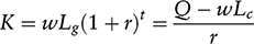 (1.1)
(1.1)
where K = capital measured in terms of the consumption commodity
w = wage rate in terms of the consumption commodity
r = rate of profits (and interest)
Lg = input, t periods ago, of labour required to produce a unit of equipment, where t is the gestation period of investmentFootnote 7
and Q = output of consumption good when Lc men work with a unit of equipment (which is assumed to last forever)
Capital in terms of labour time (KL) therefore is
 (1.2)
(1.2)
Given Lg, KL is seen to be a simple increasing function of r.
All known techniques – sets of equipment producing final outputs of the consumption good – now may be ordered according to the sizes of their outputs per head of a constant, consumption-good-trade labour force.Footnote 8 If each is ‘costed up’ at various rates of interest and expressed as amounts of KL per head, we may derive the real-factor ratio – the set of equilibrium relationships between output per head, capital in terms of labour time (or real capital, as Joan Robinson dubs it) and all conceivable wage rates. Corresponding to each equipment will be the relationship
 (1.3)
(1.3)
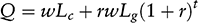
so that
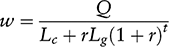 (1.4)
(1.4)
(Notice that expression (1.4) is also implied by the two sides of the equality of expression (1.1).) For any given value of w (⩽Q/Lc = wmax, which prevails when r = 0 and is the consumption good output per head of each technique), we may find the highest value of r associated with this value of w and this equipment. This reflects the view that if the equipment were viable at a given wage rate, so that it was in fact in use on the relevant island, the forces of competition would ensure that the rate of profits which exhausted the product would in fact be paid. (Whether the implied distribution of income would be such as to ensure that the product was in fact consumed is a Keynesian effective demand puzzle banished completely from our analysis, but see below, Chapter 3, pp. 104–10.)
The costing and valuation process is repeated for all equipments, ws and rs and then the relationship between output per head and real capital is plotted to give Joan Robinson’s version of the aggregate production function – her pseudo-production function – which has, as we see below in Fig. 1.1, a rather bizarre appearance relative to the smooth curves of the textbooks. Points on it should be regarded as positions of long-period stationary equilibrium which may be compared one with another since capital and output are all measured in units which allow corresponding comparisons. However, movements up and along it may not be regarded as processes occurring in historical time, the results of actual accumulation, rises in wage rates and falls in rates of profits.
It is an absurd, though unfortunately common, error to suppose that substitution between labour and capital is exhibited by a movement from one point to another along a pseudo-production function (see, for example, Reference SolowSolow [1970]). Each point represents a situation in which prices and wages have been expected, over a long past, to be what they are today, so that all investments have been made in the form that promises to yield the maximum net return to the investor. The effect of a change in factor prices cannot be discussed in these terms. Time, so to say, runs at right angles to the page at each point on the curve. To move from one point to another we would have either to rewrite past history or to embark upon a long future.
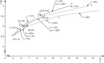
Fig. 1.1 Joan Robinson’s ‘pseudo-production function’
Moreover, as we shall see, neither the wage rate nor the reward to capital can be obtained by suitable partial differentiation of the factor–ratio relationship.
Table 1.1 contains the engineering data associated with four possible equipments, numbered 1 to 4, and an indefinite number of islands, each of which contains four men, all of whom are the current labour force of the consumption-good trade. It may be seen that the productivity of men working with equipment 1 is lowest – two and a half units of consumption good per head per period – as are the input of labour needed to make it – 20 units – and the length of its gestation period (it is in fact an instant machine). Men working with equipment 4, which requires the greatest input of labour (40.216 units) and has the longest gestation period (four periods), are the most productive (four units of consumption good per head).
Table 1.1 Engineering data on four equipments with a consumption-good-trade labour force of four men
| Equipment | Lc | Q | Q/Le | Lg | t |
|---|---|---|---|---|---|
| 1 | 4 | 10 | 2½ | 20 | 0 |
| 2 | 4 | 12 | 3 | 22.924 | 1 |
| 3 | 4 | 14 | 3½ | 29.840 | 2 |
| 4 | 4 | 16 | 4 | 40.216 | 4 |
In Table 1.2, the values of the rates of profits and real capital (in total and per head) associated with arbitrarily given wage rates in the range of one to four units of consumption good per head per period are shown. (The figures are approximate only, having been obtained from figure A1 on p. 126 of Reference ChampernowneChampernowne [1953–4].)
Table 1.2 Wage rate, rate of profits, real capital in total and per head, equipments 1–4
| Equipment: | 1 | 2 | 3 | 4 | ||||||||
|---|---|---|---|---|---|---|---|---|---|---|---|---|
| w | r | KL | KL/Lc | r | KL | KL/Lc | r | KL | KL/Lc | r | KL | KL/Lc |
| 1.000 | [30] | 20 | 5 | 27 | 29.1 | 7.3 | 22 | 44.4 | 11.1 | 16 | 72.8 | 18.2 |
| 1.250 | [20] | 20 | 5 | [20] | 27.5 | 6.9 | 17 | 40.8 | 10.2 | 13 | 65.6 | 16.4 |
| 1.500 | 12 | 20 | 5 | [15] | 26.4 | 6.6 | 13 | 38.1 | 9.5 | 10 | 58.9 | 14.7 |
| 1.837 | 7 | 20 | 5 | [10] | 25.2 | 6.3 | [10] | 36.1 | 9.0 | 8 | 54.7 | 13.7 |
| 2.000 | 5 | 20 | 5 | 8 | 24.8 | 6.2 | [9] | 35.5 | 8.9 | 7 | 52.7 | 13.2 |
| 2.481 | 0+ | 20 | 5 | 4 | 23.8 | 6.0 | [5] | 32.9 | 8.4 | [5] | 48.9 | 12.2 |
| 3.000 | n.a. | — | — | 0 | 22.9 | 5.7 | 2 | 31.0 | 7.8 | [3] | 45.3 | 11.3 |
| 4.000 | n.a. | — | — | n.a. | — | — | n.a. | — | — | 0 | 40.2 | 10.1 |
Note: square brackets indicate most or equi-most profitable equipments and corresponding values of r at given values of w.
It may be seen that at the wage rates of 1.25, 1.837 and 2.481, equipments 1 and 2, 2 and 3, and 3 and 4, respectively, are the equi-most profitable, at rates of profits of 20, 10 and 5 per cent, respectively. In between, only one type of equipment is the most profitable; for example, at a wage rate of 1.5 it is equipment 2 at a rate of profits of 15 per cent. If, therefore, we were to land on an island in which an equi-most-profitable wage rate rules, we could find the four men equipped either with all of one type of equipment, or all of the other, or with any possible combination of the two types in between (because of the assumption of complete divisibility allied with constant returns to scale). Thus when we draw the real factor ratio ‘curve’ (or pseudo-production function) (see Fig. 1.1), we get a continuous relationship between Q/Lc and KL/Lc – albeit with zigzags at the points where we cross from one island to another – even though the productivities of the men working with the different equipments differ by discrete amounts. (As Reference SolowSolow [1956a], p. 106, quipped, ‘Everyone who invents linear programming these days seems charmed by it.’) As well as showing, in unbroken lines, the possible positions of long-period stationary equilibrium – what we might hope to discover from an expedition to the islands – we also show, as dotted lines, the relationships between the outputs per head of the various equipments and the values of real capital per head when r is kept constant – what Joan Robinson calls productivity curves. We show three, those for rates of profits of 5, 10 and 20 per cent respectively.Footnote 9 Along the upward-sloping sections of the pseudo-production function, for example, from 2 to 3 along the relevant segment of the 10 per cent rate of profits productivity curve in Fig. 1.1, we gradually move from islands completely equipped with 2 to islands completely equipped with 3, passing on the way those equipped with all possible combinations in between. It is we who are moving, though, not the islands. A horizontal movement (again by us), for example, from 2 to 2 along the unbroken line in Fig. 1.1, reflects travelling from an island which is completely equipped with 2 at a rate of profits of 20 per cent to one which is completely equipped with 2 at a rate of profits of 10 per cent, passing on the way islands completely equipped with 2 at all possible values of rates of profits in between 10 and 20 per cent (one rate of profits only, of course, on each).
It has been stressed that an implication of Joan Robinson’s definition of equilibrium is that points on the pseudo-production function are equilibrium positions and that comparisons between points are just that, comparisons of one equilibrium position with another. The comparisons are certainly not a description of a process – a change – whereby accumulation occurs and new, or, rather, different techniques (technical progress is ruled out by assumption) replace old ones as a result, for example, of changes in relative factor prices. Moreover, a point which has been reiterated again and again in the literature by neo-Keynesians, especially by Joan Robinson, is that the application of results obtained from such equilibrium comparisons to long-period analyses of actual changes can be, at the least, most seriously misleading and, usually, just plain wrong. This fact vitiates many analyses of the past and, to be fair, has been countered in recent years by an enormous growth of models in which out-of-equilibrium processes are explicitly analysed, often (but not exclusively) by neo-neoclassical economists equipped with the appropriate techniques to do so.Footnote 10
The Missing Link, Champernowne-Style
Reference ChampernowneChampernowne [1953–4] accepted the logic of Joan Robinson’s approach and measure but objected to the possibility that the same physical capital could have a different value as between two situations ‘merely’ because it was associated with a different set of equilibrium rates of wages and profits. He felt it offended against the Gertrude Stein dictum (also Solow’s) that a spade a spade is is a spade …
It doesn’t seem to bother her much that on [her] definition two physically identical outfits of capital equipment can represent different amounts of ‘capital’. It wouldn’t bother me either except that from the point of view of production two identical plants represent two identical plants.
This objection is valid from the point of view of the theory of production, i.e. the ability to predict the rate of flow of output from a knowledge of factor supplies, but it is neither valid nor relevant for ‘capital’ viewed as value property, i.e. as reflecting the institutions of capitalist society. There is a real difference between the two situations and value capital ought to reflect it. The economic significance of a given plant may vary from one economic environment to another.
Nevertheless Champernowne appears to have been searching for a unit which could do both tricks at the same time. Thus he further felt it would be convenient – and more in keeping with the orthodox neoclassical tradition – to have a measure of capital such that the rewards to the factors of production could be obtained by partial differentiation of the relationship between output and capital (so measured), on the one hand, and labour, on the other. Furthermore, despite the strictures on using comparisons to analyse processes, he was keen to analyse the process of accumulation and deepening, tracing the development of capitalism over time, approaching its ‘crisis’ as real wages rose and rates of profits fell. Even if, in fact, equilibrium were ruptured repeatedly, Champernowne hoped to make the process slow enough to proceed as if this had not occurred, to measure capital each step on the way and to provide a means of comparing capital stocks over time as well as between different situations of stationary equilibrium.
Such an all-purpose measure is provided in a chain index whereby the ‘normal’ concave relationship between output per head of a constant labour force and capital per head would be established, provided that any one technique, having been the most profitable or equi-so at a given rate or range of interest rates, could never reappear again at another rate or range of rates, and that, of two techniques which are equi-profitable at a given rate of interest, it is the one with the higher output per head and higher value of capital per head that is the more profitable at a lower rate of interest. (The significance of these provisos will emerge in the discussion of the double-switching and capital-reversing debate in Chapter 4 below. Reference ChampernowneChampernowne [1953–4] examined the case where the provisos do not hold in the appendix to his article, see pp. 128–30.)
We return to the islands of stationary equilibrium involving the possible uses of techniques (= equipments) 1 to 4. In Fig. 1.2 we plot the various wage-rate–rate-of-profits trade-offs corresponding to each technique (their respective equations (1.4), see p. 25 above.)Footnote 11 The w–r trade-off of technique 1 intersects that of technique 2 at P12 and that of technique 2 intersects that of technique 3 at P23. At P12, where techniques 1 and 2 are equi-profitable (at a wage rate, w12, of 1.25 and a rate of profits, r12, of 20 per cent), the ratio of their (total)Footnote 12 capital values in terms of either the consumption commodity or in labour time (it makes no difference), as given by their respective equations (1.1) (see p. 24 above), is 20:28. (The ratio obtained from measuring capital in terms of the consumption good is
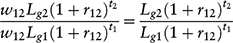
which is the ratio of their real-capital values.) At P23 (where w23 = 1.837, r23 = 10 per cent), the corresponding ratio for the capital values of 2 to 3 is 25:36. Then the chain index of capital whereby consecutive pairs of techniques are comparable one with another is
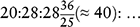
This series of index numbers shows the changes in the ‘quantity’ of capital after the effects on the value of capital of different rates of wages and profits have been removed. The discerning reader will have noted that the values of the first two links in the chain in fact correspond to the values, measured in labour time, of the total capital stocks of equipments 1 and 2 (then 2 and 3) when they are equi-profitable at a rate of profits of 20 per cent (then, for 2 and 3, 10 per cent), see Tables 1.1 and 1.2 above. The base of our index is, therefore, the real-capital value of equipment 1 at a rate of profits of 20 per cent. However, even if the two measures of capital start off from the same base, they immediately part company, as the values of real capital are absolute values whereas the others are spliced or chained indexes obtained by linking on consecutive relative changes at their appropriate places.
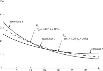
Fig. 1.2 w–r trade-offs of techniques 1–3 with resulting w–r trade-off envelope
Output may now be expressed as a unique function of labour and chain index capital, and the rewards of the factors of production correspond to the partial derivatives of the appropriate branches of the function. (If we are dealing with discrete technologies this is only true of the ‘mixed’ stationary states in which two sets of equipment are equi-most profitable. In the ‘pure’ cases, the coefficients of the production function set the upper or lower limits to the factor prices: see Reference ChampernowneChampernowne [1953–4, p. 127].) The partial derivative of output with respect to labour equals the equilibrium wage rate and the partial derivative of output with respect to capital equals the equilibrium rate of profits multiplied by the ‘price’ of ‘capital’. The price itself is a chain index price since the chain index removes, as it were, the ‘quantity’ of capital from the coefficient of the capital term. In effect Champernowne has removed the ‘zigs’ – the horizontal stretches – from Joan Robinson’s real-factor-ratio curve in Fig. 1.1, and changed the slopes of the ‘zags’ – the upward-sloping stretches – so that they now equal the relevant equilibrium values of the ‘price’ of ‘capital’.
The chain index method is not, however, confined to the case of discrete technologies. Champernowne gives an example containing a continuous spectrum of techniques and shows that we may always value consecutive techniques at common rates of profits and real-wage rates, even if each is the only technique most profitable at its r and w. When he examines accumulation he uses current factor prices for valuation purposes at any moment of time and he argues that we may make the errors as small as we like by decreasing the size of the links in the chain. When he compares stationary states, in the continuous case he uses lower rs and higher ws for linking purposes: see Reference ChampernowneChampernowne [1953–4], p. 115. Finally, it should be noted – and noted well – that the chain index method depends upon knowing from elsewhere and already, the rate of profits or wage rate and calculating a price of output which corresponds to the unit cost of producing it. Capital is therefore not measured in a unit which is independent of distribution and prices.
A verbal explanation of the properties of the chain index capital production function is as follows: consider, say, equipments 1 and 2 which we know are equi-most profitable at the rate of profits of r12 (=20 per cent). Equipment 2 allows a higher output per head (3 units) than equipment 1
 units). Let island A employ quantities 5 of 1 and 7 of 2, measured in terms of the chain index; island B uses 5+1 (= 6) of 1 and 7−1 (= 6) of 2 (constant returns to scale allow divisibility of this nature). Then the costs at wage rate w12 (= 1.25), and rate of profits r12 (= 20 per cent), of the total sets of equipment are the same on both islands, namely, 12 chain index units each, so that the interest bills (or normal profits payments) are the same on both islands also. Therefore the difference between the total product flows of the two islands (
 units of the consumption good) must equal the difference between their total wage bills
 . Thus the extra product of the island with the greater amount of labour, B in this case,Footnote 13 is just sufficient to pay the wages of the extra labour at the competitive wage rate. That is to say, the wage of labour (1.25) equals the marginal product of labour
 , the ‘quantity’ of capital being held constant. (But see pp. 45–47 below, where it is shown that
 does not correspond to the traditional definition of a marginal product.)
We now show that the partial derivatives of the appropriate branches of the production function, when we consider mixed stationary states, do indeed equal the equilibrium factor prices. Consider the two branches that correspond to the islands with mixed amounts of equipments 1 and 2, and 2 and 3 respectively. Following Reference ChampernowneChampernowne [1953–4], pp. 126–8, they may be written (in total form) as:
1, 2
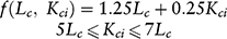
2, 3
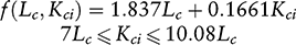 (1.5)
(1.5)
where Kci = capital, chain index measure, and the inequalities show the ranges of the values of capital within which the expressions apply, e.g., the range 20–28 corresponds to the 1, 2 branch.
The values of the coefficients of the Lc and Kci terms were derived as follows: consider, for example, the 2, 3 branch,
2, 3

We know that:

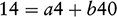 (1.6)
(1.6)
where a and b are the unknown coefficients and the values of output, labour and capital (chain index measure) corresponding to equipments 2 and 3, and at the rates of wages and profits where the two equipments co-exist (see pp. 31–32 above) have been inserted. Solving expression (1.6) for a and b gives the values of the coefficients of the 2, 3 branch.
Partially differentiating the branches with respect to labour, for example, does indeed give marginal products of labour equal to the appropriate equilibrium wage rates. The values of the coefficients of the capital terms are, of course, affected by the base from which the chain index starts. The interested reader may check for himself that the choice of a base, either one of capital valued in terms of the consumption good or for real does not affect the coefficients of the labour terms. If, however, real capital were used in all branches, it would not be true in general that the respective capital and labour coefficients equalled the equilibrium factor prices. In Fig. 1.3 we show the three branches of the production function where output per man is measured in terms of the consumption good and capital per man is measured as a chain index.
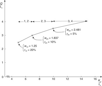
Fig. 1.3 Champernowne’s production function
Swan’s Way
In Swan’s model of economic growth, Reference SwanSwan [1956], capital–labour ratios need to change considerably as accumulation occurs over time, in order that both stable equilibrium capital–output and capital–labour ratios may be re-established following a change in a parameter, for example, the saving ratio. In this manner, considerable processes occur, or, rather, are analysed. Moreover, he uses a Cobb–Douglas production function, and assumes that saving determines investment, and that there are constant returns to scale, full employment, static expectations and perfect competition, so that the wage of labour equals its full-employment marginal product and the rate of profits on capital equals its marginal product. (Also, of course, the shares of labour and capital in the national product equal the ratios of their respective full-employment marginal to average products, which, in turn, equal the respective exponents (also output elasticities) of the production function.)Footnote 14
Having carried out in the text of his article an analysis which ‘takes a neoclassical form’ so enjoying ‘the neoclassical as well as the Ricardian vice’, Swan spells out in the appendix, in ‘a back foremost’ procedure, the assumptions that would justify the approach, the scarecrow that would keep off both ‘the index number birds and Joan Robinson herself’. His first line of defence is to suppose that capital consists of meccano sets which can be costlessly and timelessly transformed into any desired form, as given by the latest booklet of instructions (so incorporating technical progress), in order to cooperate with labour in response to the pull of changes in relative factor prices and to technical advances. The relative prices of products (including meccano sets) never change, no matter how rates of wages and profits (and, sometimes, rents, when land, which we ignore, is considered) do.
In this way the aggregation of heterogeneous items of capital, both as cross-sections and over time, where they are both ‘infinitely durable and instantaneously adaptable’, is possible in terms of their own technical unit and ‘the basic model of [his] text could be rigorously established in a form which deceived nobody’ – an answer which proceeds by abolishing the question. For, with malleability, disappointed expectations and imperfect foresight can be avoided since the capital stock can be made into any form that is wanted and adapted to any labour supply that is forthcoming.
Thus it is hoped that the long-run implications of capital–labour substitution may be analysed independently of any troublesome short-run Keynesian and other puzzles. As Reference FergusonFerguson [1969] puts it, the tendencies inherent in the Marshallian long run may be analysed free of interference from other, for this purpose, he believes, irrelevant factors. His argument has been severely criticized in, for example, Reference RobinsonRobinson [1970a], Reference HarcourtHarcourt [1970b] and Chapter 2, pp. 67–69, below. The main point of the criticism is that all economic decisions are of necessity made in the short run, where all actions are of necessity also, even though some decisions, e.g., those relating to investment, relate to longer horizons than do others, e.g., those relating to output. We find in Swan’s appendix perhaps the first and certainly the clearest statement of the notorious malleability assumption which underlies many neoclassical growth models and econometric exercises, for example Reference SwanSwan [1956], Reference SolowSolow [1956b, Reference Solow1957], Reference MeadeMeade [1961].
By measuring capital in terms of its own technical unit (and by assuming that the quantity of capital in terms of this unit is uniquely associated with, say, the annual flow of services from it, measured in machine years), it is in the appropriate form for inclusion in a production function viewed as an engineering description of the flow of output which may be expected from the inputs of certain flows of man and machine years: on this, see Reference Bruno, Burmeister and SheshinskiBruno, Burmeister and Sheshinski [1968]. The marginal product of capital, so measured, is equal to the rate of profits multiplied by the price of the technical unit of capital in terms of product (p). But if this price does not change when accumulation occurs, as Swan assumes, capital may also be measured in value units, in which case its marginal product equals the rate of profits. Thus, in equilibrium,
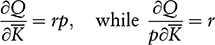 (1.7)
(1.7)
where Q = product and
 = capital measured in terms of its technical unit. As Q and
 are measured in the same units, the units cancel, leaving a pure number which is the dimension of the rate of profits.
As Reference HicksHicks [1965] has pointed out (also Reference SwanSwan [1956]), outside a one-commodity world the price of capital services – its rental – is the rate of profits multiplied by the price per unit of capital goods. In a one-commodity world the rate of profits and the marginal product of capital, one a pure number, the other an instantaneous rate of change, can be equal and the valuation problem can be dodged. Malleability cannot, however, because we must suppose that capital can change its form (or be viewed ‘as if’ it could) in order to identify its marginal product: see Reference SamuelsonSamuelson [1962], and Chapter 4 below, also the appendix to Reference PasinettiPasinetti’s [1969] article where this point is admirably explained. In a world of heterogeneous capital goods, valuation is needed so that we have a sum to which to apply the rate of profits. As we shall see below in Chapter 4, this rate of profits is not in general equal to the marginal product of ‘capital’.
The neoclassical procedure can be regarded as an examination of virtual displacements around an equilibrium point, so that any relative price changes may be ignored and capital may be measured in terms of ‘an equilibrium dollar’s worth’. With this procedure it is legitimate – and essential – for individual economic actors to take all prices as given (they are, after all, price-takers) and it is market forces – the overall outcome of their individual but, consciously anyway, uncoordinated actions – which are responsible for actual price changes, changes which cease, by definition, at equilibrium. Moreover, any accumulation which is conceived to have taken place is marginal so that any change in the value of meccano sets in terms of product is confined to this marginal addition, and so may be ignored.
The trouble is that when either comparisons are made between different economies with different equilibrium wages, rates of profits and factor endowments – what Swan calls ‘structural comparisons in the large’ – or, far worse, when accumulation is analysed, these equilibrium points with all their accompanying (instantaneous) rates of change cannot be extended into visible curves associated with the same equilibrium values. An enormous revaluation of existing capital stocks occurs whenever an actual change (as opposed to a virtual one), no matter how small, is contemplated. Hence the need either for meccano sets (and the accompanying unacceptable assumption of perfectly timeless and costless malleability) or for resort to Champernowne’s chain index which both he and Swan argue also allows an analysis of slow accumulation, in Champernowne’s case, without technical progress.Footnote 15 The operative word is slow, so that it takes a long time to pass between points which are far apart, and the conditions necessary for equilibrium at each point have a ‘reasonable chance’ of being established as the economy passes from one point to another. This particular act of faith has been a feature of many subsequent growth models constructed by true neoclassical believers, see, for example, Reference MeadeMeade [1961].
In Champernowne’s example, where the function is assumed to be single-valued and well-behaved, the progress is from a high rate of profits, low wage rate, low-productivity technique to a low rate of profits, high wage rate, high-productivity method: see Reference ChampernowneChampernowne [1953–4], pp. 118–19. The Champernowne method is to use a series of snap-shots of stationary states that are reasonably close together. He supposes that enough accumulation has occurred to move the economy from one state to another, the amount of accumulation being analysed by the chain index method, so that the differences between the consecutive islands are treated as if they were equivalent to the changes occurring over time: ‘… the interest of a comparison of a sequence of stationary states is due to the presumption that this will give a first approximation to a comparison of successive positions in a slow process of steady accumulation’ (p. 119). Champernowne adds that the presumption is more likely to be realized in the case of continuous technologies than in the case of discrete ones. During his discussion of this viewpoint, Champernowne cites an example whereby measuring capital in terms of labour time (what he calls JR units), associates a situation requiring positive net investment with one of apparent negative net investment, i.e. a reduction in real capital per head. This puzzle occurs because of a negative bias in the measurement of net investment due to the fall in the rate of interest; it disappears when the chain index method is used.
Wicksell Effects, Price and Real, Exposed
In the last two sections of the appendix of Reference SwanSwan [1956], Swan discusses the nature of the Wicksell effect, which Joan Robinson had commented on in her article, Reference RobinsonRobinson [1953–4], and returned to in more detail in her book, Reference RobinsonRobinson [1956], and later articles, Reference RobinsonRobinson [1958] and Reference Robinson and NaqviRobinson and Naqvi [1967]. In particular, Swan is concerned to show in terms of Wicksell’s own examples (the point-input–point-output case and the analysis of Åckerman’s problem, see Reference SwanSwan [1956], pp. 352–61) that ‘the Wicksell Effect is nothing but an inventory revaluation’ (p. 355). In establishing this point, he accused Joan Robinson of confusing the change in the value of a stock of capital with the value of the change, a charge which she understandably took rather amiss, see Reference RobinsonRobinson [1957], p. 107 n6. Wicksell demonstrated that an increase in social capital is partly ‘absorbed by increased wages … so that only the residue … is really effective as far as a rise in production is concerned’. As Swan shows (see pp. 352–53) this implies that the marginal product of capital (in Wicksell’s point-input–point-output case) is less than the rate of interest, an obstacle in the way of the acceptance of ‘von Thünen’s thesis’ (which was its main interest to Wicksell).
In the modern literature the ‘real’ and ‘financial’ aspects of an increase in social capital have come to be discussed under the heading of real and price Wicksell effects, respectively. The wage-rate–rate-of-profits trade-off analysis developed earlier in the chapter allows a simple discussion of this distinction and allows us to show in a simple way what Swan had in mind when he described the (price) Wicksell effect as an inventory revaluation.
The price Wicksell effect relates to changes in the value of capital as w and r change their values but techniques do not change, i.e. it is associated with the w–r relationship that corresponds to one technique. Real Wicksell effects relate to changes in the value of capital associated with changes in techniques as w and r take on different values, i.e. they are differences in the values of capital at (or, rather, very near) switch points on the envelope of the w–r relationships. Switch points are the intersection points where two techniques are equi-most profitable. Both effects reflect the influence, through w and r, of the ‘time’ pattern of inputs of production, but real effects reflect in addition changes in production methods, i.e. changes which reflect real production potentials, not just their market values.
Consider an economy-wide technique which has a net output per head of a consumption good, q. Assume that we are in a stationary state (which is formally equivalent to what Reference GaregnaniGaregnani [1970a] calls an integrated consumption-good industry) and that capital goods last forever. Then
 (1.8)
(1.8)
where all values are measured in consumption-good units per head, so that
 (1.9)
(1.9)
When r = 0, q = wmax, the maximum wage which is also output per head.
Because of our assumptions, q = wmax for all values of r. If we had more than one consumption good, or were considering a growing economy in which net investment formed part of the national product, q = wmax would hold only when r = 0 and net investment were either zero or the same good, because the value of q is affected by the relative prices of capital goods in terms of consumption goods which are themselves affected by the value of r.Footnote 16
We write the w–r relationship as
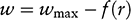 (1.10)
where, for r = 0, f(0) = 0 and f′(r)>0, i.e. the w–r ‘curve’ slopes downward. Then
 (1.11)
 (1.12)
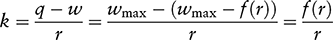
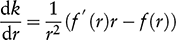
with
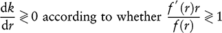 (1.13)
Expression (1.13) provides a very simple method by which we may determine the relationship between the shapes (and slopes) of w–r curves and dk/dr. Consider a w–r curve which is concave to the origin, and for which, wmax = OS (see Fig. 1.4). Consider any value of r, say r1; draw a tangent at P (which is the point on the w–r curve corresponding to r1) and extend it to meet the w axis at Q. Draw a horizontal line from P to join the w axis at R. Then RQ = f′(r1)r1 and RS = f(r1). It may be seen that RQ/RS>1, which by expression (1.13) implies that dk/dr > 0. That is to say, a w–r curve which is concave to the origin implies a negative price Wicksell effect – the value of capital is lower, the lower is the value of r, the inventory revaluation is negative. By exactly analogous reasoning we may show that a w–r relationship which is convex to the origin implies a positive price Wicksell effect and that a straight-line one implies a zero or neutral price Wicksell effect, a crucial result which we shall meet again in Chapter 4.Footnote 17
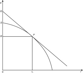
Fig. 1.4 Negative price Wicksell effect
The following simple diagrams, in which the relationship, k = (q−w)/r, is used, are an alternative means of making the same points. Consider a w–r curve that is concave to the origin and the values of k associated with r1 and r2 in Fig. 1.5a. Clearly k1 < k2, i.e. the value of k is lower, the lower is the value of r – a negative price Wicksell effect. The other two possibilities are shown in Figs 1.5b and 1.5c.Footnote 18
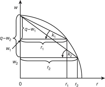
Fig. 1.5a Negative price Wicksell effect
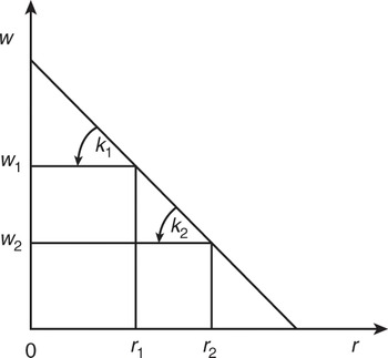
Fig. 1.5b Neutral price Wicksell effect
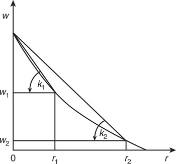
Fig. 1.5c Positive price Wicksell effect
We may identify a positive real Wicksell effect as one in which a technique with a higher output per head and higher value of capital per head at a switch point is chosen at a rate of profits just below the switch-point rate of profits. Thus, in Fig. 1.6, technique b, having been equi-profitable with a at rab, becomes the more profitable at rates of interest <rab. The value of capital associated with b at rab,kb{ = (wb max− wab)/rab}, exceeds the corresponding value of capital associated with a, ka{ = (wa max − wab)/rab}. (Both allow the same wage rate and the same rate of profits to be paid but as labour equipped with b is more productive than that equipped with a (wb max > wa max), a must have a lower value of k in order that its smaller amount of profit, when expressed as a proportion of ka, equals rab.) As the price Wicksell effect is negative for a and neutral for b, the value of capital for b for rates of profits <rab will also continue to exceed those for a, indeed, by greater and greater amounts. At rba, a negative real Wicksell effect occurs.
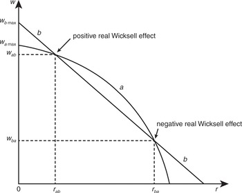
Fig. 1.6 Real Wicksell effects
The differences just below the switch points reflect both differences in productivity as between the two methods and valuation or price effects. It is only at switch points that the differences can be said, in general, to be entirely ‘real’. For it is only at switch points that the wage and profits rates are the same for both methods so that any difference between the values of their ks must be attributable to the differences in the productivities of the methods. Anywhere else, though one factor price will be common to both, the other one will not, it being greater for the technique which is in use, i.e. is on the w–r envelope. (Moving horizontally across the diagram, it is w which is common; moving vertically it is r.) If both relationships are straight lines, though, the differences between their ks are nevertheless ‘real’ away from switch points because the price effects of both are neutral. Finally, if one w–r relationship is a straight line and the other curved, as in Fig. 1.6, or if both are curved, the changes in the differences between the ks away from the switch points are entirely price Wicksell effects.
At switch points such as rab and rba, the careful reader will notice that as the wage rates and the rates of profits are the same for both techniques, the additional amount of product associated with the more productive technique, when expressed as a proportion of the differences in capital values as between the two techniques, is equal to the equilibrium rate of profits.
Thus
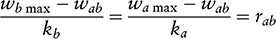 (1.14)
i.e.

i.e.
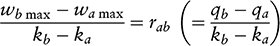 (1.15)
It would be tempting to call the ratio, (qb–qa)/(kb–ka) (= Δq/Δk), the marginal product of capital and so deduce that it equals the – externally given – rate of profits. It would also be wrong to do so as Reference PasinettiPasinetti [1969], pp. 529–31, shows with great insight and clarity. The marginal product of capital, as defined in the traditional literature, is not, he argues, the (limiting) ratio of the increment of output to the increment of capital when two techniques are equi-profitable, i.e. the rate of profits is unchanged, and the proportions in which the techniques are used are changed. It is, rather, the (limiting) ratio of the corresponding increments when we compare two techniques which are the most profitable at different rates of profits, not at one and the same one.
That is to say, in the traditional case, we consider the implications of a change in the rate of profits (which in the limit becomes infinitesimally small) for the ratio of the change in output to the change in the ‘quantity of capital’. In the case above, though, we consider the implications, for the (limiting) ratio of the increments, of a change in the proportions in which two equi-profitable techniques are combined, the rate of profits remaining unchanged – as does, of course, the amount of labour in both cases. The differences between the two concepts highlight the crucial point that if the marginal product of capital is to be part of an explanation of the rate of profits itself, the changes in the ‘quantities’ as we go from one technique to another must themselves be independent of changes in the rate of profits. ‘Capital’, like labour, has to be measured in a unit which is independent of distribution and prices. Clearly in the definition above, whereby Δq/Δk = r, the seeming independence is only superficially so because r, by assumption, does not change.
The above considerations may appear to raise doubts about the verbal explanation, see pp. 33–35 above, that when we use the chain index method of measuring capital, the marginal product of labour equals the equilibrium wage rate. The answer is that it should raise doubts, very considerable ones, even though the chain index method is specifically designed to deal with this point, especially in the case of a continuous spectrum of techniques whereby we obtain values of capital of techniques which are the most profitable at different rates of profits from one another.Footnote 19
Solow’s Opening Skirmish
It would be unfair – also foolhardy – to end the chapter without reference to Solow’s comment in Reference SolowSolow [1956a] on Joan Reference RobinsonRobinson’s [1953–4] article. Solow investigated the conditions under which it would be legitimate to aggregate heterogeneous capital items into a single figure, no doubt having in mind his subsequent econometric studies. He found that the conditions were very stringent – the rate at which one capital good could be substituted for another had to be independent of the amounts of labour which subsequently would be used with each. (He discusses in this context a neoclassical model in which continuous substitution is possible, not the discrete case of Joan Robinson’s article, but he also looks at the latter towards the end of his article.) His conclusion is quoted in full below because it is an extremely clear statement of the stand that he takes in the debates that followed:
I conclude that discreteness is unlikely to help matters. Only in very special cases will it be possible to define a consistent measure of capital-in-general. Some comfort may be gleaned from the reflection that when capital–labour ratios differ widely we hardly need a subtle index to tell us so, and when differences are slight we are unlikely to believe what any particular index says.
For Solow, ‘Capital as a number is not an issue of principle. All rigorously valid results come from n-capital-good models. In particular there is no justification ever for supposing that output can be made a function of labour and the VALUE of capital whose partial derivatives do the right thing.’ Capital as a number is purely an aid to empirical work ‘and you want to get away with the smallest dimensionality possible’ (Reference SolowSolow [1969]). Had the contestants been content to leave the discussion here, the literature of the following years might have served to generate far more light – and certainly a lot less heat.


