To save content items to your account,
please confirm that you agree to abide by our usage policies.
If this is the first time you use this feature, you will be asked to authorise Cambridge Core to connect with your account.
Find out more about saving content to .
To save content items to your Kindle, first ensure no-reply@cambridge.org
is added to your Approved Personal Document E-mail List under your Personal Document Settings
on the Manage Your Content and Devices page of your Amazon account. Then enter the ‘name’ part
of your Kindle email address below.
Find out more about saving to your Kindle.
Note you can select to save to either the @free.kindle.com or @kindle.com variations.
‘@free.kindle.com’ emails are free but can only be saved to your device when it is connected to wi-fi.
‘@kindle.com’ emails can be delivered even when you are not connected to wi-fi, but note that service fees apply.
2.1 (i) A ∪ B = {1, 2, 3, 4, 5, 9}; (ii) A ∩ B = {1, 3}; (iii) A \ B = {2, 4};(iv) B \ A = {5, 9};(v) Ā = {5, 9}, and B = {2, 4}
2.2 (i) A ∪ B = {0, 1, 2, 3, 5, 6, 9};(ii) A ∩ B = {5}; (iii) A \ B = {0, 2, 6};(iv) B \ A = {1, 3, 9}
2.3 (i) For example see the top part of Figure 2.3; (ii) see Figure 2.2, where A and B are interchanged.
2.4 A ∪ B = R
2.5 A ∪ B = R
2.6 A ∩ B = 1, 2, 3, 4, 5
2.7 A ∩ B = ø
2.8 A ∪ B ∩ C = Z+
2.9 A ∪ B ∩ C = {0, Z-}
2.10 ΩDecimal = {0, 1, 2, 3, 4, 5, 6, 7, 8, 9}
2.11 {red, green, blue}
2.12 C
2.13 Z
2.14 {x|5 < x < 10}
2.15 {x |x ∈ R}
3. Probability
3.1 4/52 = 0.077 to 3 s.f.
3.2 0.45%
3.3 20/52 = 0.385 to 3 s.f.
3.4 The probability of the getting an ace followed by a 10 point card, where the other player also gets a 10 point card is 0.72%. The probability of getting an ace followed by a 10 point card, where the other player gets a card with a different value is 1.69%. The total probability of being dealt an ace followed by a 10 point card is the sum: 2.41%.
The foundations of science are built upon centuries of careful observation. These constitute measurements that are interpreted in terms of hypotheses, models, and ultimately well-tested theories that may stand the test of time for only a few years or for centuries. In order to understand what a single measurement means we need to appreciate a diverse range of statistical methods. Without such an appreciation it would be impossible for scientific method to turn observations of nature into theories that describe the behaviour of the Universe from sub-atomic to cosmic scales. In other words science would be impracticable without statistical data analysis. The data analysis principles underpinning scientific method pervade our everyday lives, from the use of statistics we are subjected to through advertising to the smooth operation of SPAM filters that we take for granted as we read our e-mail. These methods also impact upon the wider economy, as some areas of the financial industry use data mining and other statistical techniques to predict trading performance or to perform risk analysis for insurance purposes.
This book evolved from a one-semester advanced undergraduate course on statistical data analysis for physics students at Queen Mary, University of London with the aim of covering the rudimentary techniques required for many disciplines, as well as some of the more advanced topics that can be employed when dealing with limited data samples. This has been written by a physicist with a non-specialist audience in mind. This is not a statistics book for statisticians, and references have been provided for the interested reader to refer to for more rigorous treatment of the techniques discussed here.
The probability of something occurring is the quantification of the chance of observing a particular outcome given a single event. The event itself may be the result of a single experiment, or one single data point collected by an un-repeatable experiment. We refer to a single event or an ensemble of events as data, and the way we refer to data implies if data is singular or plural. If we quantify the probability of a repeatable experiment, then this understanding can be used to make predictions of the outcomes of future experiments. We cannot predict the outcome of a given experiment with certainty; however, we can assign a level of confidence to our predictions that incorporates the uncertainty from our previous knowledge and any information of the limitations of the experiment to be performed.
Consider the following. A scientist builds an experiment with two distinct outputs A and B. Having prepared the experiment, the apparatus is configured to always return the result A, and never return the result B. If the experiment is performed over and over again one will always obtain the result A with certainty. The probability of obtaining this result is 1.0 (100%). The result B will never be observed, and so the probability of obtaining that result is 0.0 (0%).
The publication in 1890 of the two-volume Scientific Papers of James Clerk Maxwell, edited by W. D. Niven, was one of the two objects of a committee formed 'for the purpose of securing a fitting memorial of him' (the other object being the commissioning of a marble bust for the Cavendish Laboratory). Before his death in 1879 at the age of 48, Clerk Maxwell had made major contributions to many areas of theoretical physics and mathematics, not least his discoveries in the fields of electromagnetism and of the kinetic theory of gases, which have been regarded as laying the foundations of all modern physics. He is generally considered the third most important physicist of all time, after Newton and Einstein. These collected shorter works, beginning with a paper written at the age of 15, show the wide range of Clerk Maxwell's interests across mathematics, physics and chemistry.
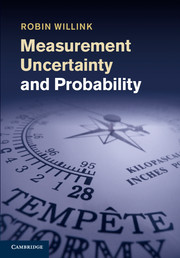
A measurement result is incomplete without a statement of its 'uncertainty' or 'margin of error'. But what does this statement actually tell us? By examining the practical meaning of probability, this book discusses what is meant by a '95 percent interval of measurement uncertainty', and how such an interval can be calculated. The book argues that the concept of an unknown 'target value' is essential if probability is to be used as a tool for evaluating measurement uncertainty. It uses statistical concepts, such as a conditional confidence interval, to present 'extended' classical methods for evaluating measurement uncertainty. The use of the Monte Carlo principle for the simulation of experiments is described. Useful for researchers and graduate students, the book also discusses other philosophies relating to the evaluation of measurement uncertainty. It employs clear notation and language to avoid the confusion that exists in this controversial field of science.
A First Course in Computational Algebraic Geometry is designed for young students with some background in algebra who wish to perform their first experiments in computational geometry. Originating from a course taught at the African Institute for Mathematical Sciences, the book gives a compact presentation of the basic theory, with particular emphasis on explicit computational examples using the freely available computer algebra system, Singular. Readers will quickly gain the confidence to begin performing their own experiments.
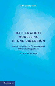
Mathematical Modelling in One Dimension demonstrates the universality of mathematical techniques through a wide variety of applications. Learn how the same mathematical idea governs loan repayments, drug accumulation in tissues or growth of a population, or how the same argument can be used to find the trajectory of a dog pursuing a hare, the trajectory of a self-guided missile or the shape of a satellite dish. The author places equal importance on difference and differential equations, showing how they complement and intertwine in describing natural phenomena.
In the previous section we saw that difference equations can be used to model quite a diverse phenomena but their applicability is limited by the fact that the system should not change between subsequent time steps. These steps can vary from fractions of a second to years or centuries but they must stay fixed in the model. On the other hand, there are numerous situations when changes can occur at all times. These include the growth of populations in which breeding is not restricted to specific seasons, motion of objects, where the velocity and acceleration may change at every instant, spread of an epidemic with no restriction on infection times, and many others. In such cases it is not feasible to model the process by relating the state of the system at a particular instant to a finite number of earlier states (although this part remains as an intermediate stage of the modelling process). Instead, we have to find relations between the rates of change of quantities relevant to the process. The rates of change typically are expressed as derivatives and thus continuous time modelling leads to differential equations which involve the derivatives of the function describing the state of the system.
In what follows we shall derive several differential equation models trying to provide continuous counterparts of some discrete systems described above.
Equations related to financial mathematics
In this section we shall provide continuous counterparts of equations (2.2) and (2.5) and compare the results.
In this chapter we first introduce discrete mathematical models of phenomena happening in the real world. We begin with some explanatory words. Apart from the simplest cases such as the compound interest equation, where the equation is a mathematical expression of rules created by ourselves, the mathematical model attempts to find equations describing events happening according to their own rules, our understanding of which is far from complete. At best, the model can be an approximation of the real world. This understanding guides the way in which we construct the model: we use the principle of economy (similar to the Ockham razor principle) to find the simplest equation which incorporates all relevant features of the modelled events. Such a model is then tested against experiment and only adjusted if we find that its description of salient properties of the real phenomenon we try to model is unsatisfactory.
This explains why we often begin modelling by fitting a linear function to the data and why such linear, or only slightly more complicated, models are commonly used, although everybody agrees that they do not properly describe the real world. The reason is that often they supply sufficient, if not exact, answers at a minimal cost. One must remember, however, that using such models is justified only if we understand their limitations and that, if necessary, are ready to move in with more fine-tuned ones.
Engineers, natural scientists and, increasingly, researchers and practitioners working in economics and other social sciences, use mathematical modelling to solve problems arising in their disciplines. There are at least two identifiable kinds of mathematical modelling. One involves translating the rules of nature or society into mathematical formulae, applying mathematical methods to analyse them and then trying to understand the implications of the obtained results for the original disciplines. The other kind is to use mathematical reasoning to solve practical industrial or engineering problems without necessarily building a mathematical theory for them.
This book is predominantly concerned with the first kind of modelling: that is, with the analysis and interpretation of models of phenomena and processes occurring in the real world. It is important to understand, however, that models only give simplified descriptions of real-life problems but, nevertheless, they can be expressed in terms of mathematical equations and thus can be solved in one way or another.