To save content items to your account,
please confirm that you agree to abide by our usage policies.
If this is the first time you use this feature, you will be asked to authorise Cambridge Core to connect with your account.
Find out more about saving content to .
To save content items to your Kindle, first ensure no-reply@cambridge.org
is added to your Approved Personal Document E-mail List under your Personal Document Settings
on the Manage Your Content and Devices page of your Amazon account. Then enter the ‘name’ part
of your Kindle email address below.
Find out more about saving to your Kindle.
Note you can select to save to either the @free.kindle.com or @kindle.com variations.
‘@free.kindle.com’ emails are free but can only be saved to your device when it is connected to wi-fi.
‘@kindle.com’ emails can be delivered even when you are not connected to wi-fi, but note that service fees apply.
In many practical applications of probability, physical situations are better described by random variables that can take on a continuum of possible values rather than a discrete number of values. Examples are the decay time of a radioactive particle, the time until the occurrence of the next earthquake in a certain region, the lifetime of a battery, the annual rainfall in London, electricity consumption in kilowatt hours, and so on. These examples make clear what the fundamental difference is between discrete random variables taking on a discrete number of values and continuous random variables taking on a continuum of values. Whereas a discrete random variable associates positive probabilities with its individual values, any individual value has probability zero for a continuous random variable. It is only meaningful to speak of the probability of a continuous random variable taking on a value in some interval. Taking the lifetime of a battery as an example, it will be intuitively clear that the probability of this lifetime taking on a specific value becomes zero when a finer and finer unit of time is used. If you can measure the heights of people with infinite precision, the height of a randomly chosen person is a continuous random variable. In reality, heights cannot be measured with infinite precision, but the mathematical analysis of the distribution of people's heights is greatly simplified when using a mathematical model in which the height of a randomly chosen person is modeled as a continuous random variable. Integral calculus is required to formulate the continuous analogue of a probability mass function of a discrete random variable.
The first purpose of this chapter is to familiarize you with the concept of the probability density of a continuous random variable. This is always a difficult concept for the beginning student. However, integral calculus enables us to give an enlightening interpretation of probability density. The second purpose of this chapter is to introduce you to important probability densities such as the uniform, exponential, gamma, Weibull, beta, normal, and lognormal densities among others. In particular, the exponential and normal distributions are treated in depth. Many practical phenomena can be modeled by these distributions, which are of fundamental importance. Many examples are given to illustrate this.
In performing a chance experiment, one is often not interested in the particular outcome that occurs but in a specific numerical value associated with that outcome. Any function that assigns a real number to each outcome in the sample space of the experiment is called a random variable. Intuitively, a random variable takes on its value by chance. The observed value, or realization, of a random variable is completely determined by the realized outcome of the chance experiment and consequently probabilities can be assigned to the possible values of the random variable.
The first purpose of this chapter is to familiarize you with the concept of a random variable and with characteristics such as the expected value and the variance of a random variable. In addition, we give rules for the expected value and the variance of a sum of random variables, including the square-root rule. These rules are easiest explained and understood in the context of discrete random variables. Such random variables can take on only a finite or countably infinite number of values (the so-called continuous random variables that can take on a continuum of values are treated in the next chapter). The second purpose of the chapter is to introduce you to important discrete random variables such as the binomial, Poisson, hypergeometric, geometric, and negative binomial random variables among others. A comprehensive discussion of these random variables is given, together with appealing examples. Much attention is given to the Poisson distribution, which is the most important discrete distribution. Unlike most other introductory texts, we consider at length the practically useful Poisson heuristic for weakly dependent trials.
Concept of a Random Variable
The concept of a random variable is always difficult for the beginner. Intuitively, a random variable is a function that takes on its value by chance. A random variable is not a variable in the traditional sense of the word and actually it is a little misleading to call it a variable. Formally, a random variable is defined as a real-valued function on the sample space of a chance experiment. A random variable X assigns a numerical value X(ω) to each element ω of the sample space.
For centuries, mankind lived with the idea that uncertainty was the domain of the gods and fell beyond the reach of human calculation. Common gambling led to the first steps toward understanding probability theory, and the colorful Italian mathematician and physician Gerolamo Cardano (1501–1575) was the first to attempt a systematic study of the calculus of probabilities. As an ardent gambler himself, Cardano wrote a handbook for fellow gamblers entitled Liber de Ludo Aleae (The Book of Games of Chance) about probabilities in games of chance like dice. He originated and introduced the concept of the set of outcomes of an experiment, and for cases in which all outcomes are equally probable, he defined the probability of any one event occurring as the ratio of the number of favorable outcomes to the total number of possible outcomes. This may seem obvious today, but in Cardano's day such an approach marked an enormous leap forward in the development of probability theory.
Nevertheless, many historians mark 1654 as the birth of the study of probability, since in that year questions posed by gamblers led to an exchange of letters between the great French mathematicians Pierre de Fermat (1601– 1665) and Blaise Pascal (1623–1662). This famous correspondence laid the groundwork for the birth of the study of probability, especially their question of how two players in a game of chance should divide the stakes if the game ends prematurely. This problem of points, which will be discussed in Chapter 3, was the catalyst that enabled probability theory to develop beyond mere combinatorial enumeration.
In 1657, the Dutch astronomer Christiaan Huygens (1629–1695) learned of the Fermat–Pascal correspondence and shortly thereafter published the book De Ratiociniis de Ludo Aleae (On Reasoning in Games of Chance), in which he worked out the concept of expected value and unified various problems that had been solved earlier by Fermat and Pascal. Huygens’ work led the field for many years until, in 1713, the Swiss mathematician Jakob Bernoulli (1654–1705) published Ars Conjectandi (The Art of Conjecturing) in which he presented the first general theory for calculating probabilities.
In previous chapters we have dealt with sequences of independent random variables. However, many random systems evolving in time involve sequences of dependent random variables. Think of the outside weather temperature on successive days, or the price of IBM stock at the end of successive trading days.Many such systems have the property that the current state alone contains sufficient information to give the probability distribution of the next state. The probability model with this feature is called a Markov chain. The concepts of state and state transition are at the heart of Markov chain analysis. The line of thinking through the concepts of state and state transition is very useful to analyze many practical problems in applied probability.
Markov chains are named after the Russian mathematician Andrey A. Markov (1856–1922), who introduced the concept of the Markov chain in a 1906 publication. In a famous paper written in 1913, he used his probability model to analyze the frequencies with which vowels and consonants occur in Pushkin's novel Eugene Onegin. Markov showed empirically that adjacent letters in Pushkin's novel are not independent but obey his theory of dependent random variables. Markov's work helped launch the modern theory of stochastic processes (a stochastic process is a collection of random variables, indexed by an ordered time variable). The characteristic property of a Markov chain is that its memory goes back only to the most recent state. Knowledge of the current state only is sufficient to describe the future development of the process. A Markov model is the simplest model for random systems evolving in time when the successive states of the system are not independent. But this model is no exception to the rule that simple models are often the most useful models for analyzing practical problems. The theory of Markov chains has applications to a wide variety of fields, including biology, physics, engineering, operations research, and computer science. Markov chains are almost everywhere in science today. A similar method as used by Andrey Markov to study the alternation of vowels and consonants in Pushkin's novel helps identify genes in DNA. Markovian language models are nowadays used in speech recognition. In physics, Markov chains are used to simulate the macrobehavior of systems made up of many interacting particles.
The concept of conditional probability lies at the heart of probability theory. It is an intuitive concept. To illustrate this, most people reason as follows to find the probability of getting two aces when two cards are selected at random from an ordinary deck of 52 cards. The probability of getting an ace on the first card is 4 52. Given that one ace is gone from the deck, the probability of getting an ace on the second card is 3 51. The sought probability is therefore 4 52 × 3 51. Letting A1 be the event that the first card is an ace and A2 the event that the second card is an ace, one intuitively applies the fundamental formula P(A1A2) = P(A1)P(A2 | A1), where P(A2 | A1) is the notation for the conditional probability that the second card will be an ace given that the first card was an ace.
The purpose of this chapter is to present the basics of conditional probability. You will learn about the multiplication rule for probabilities and the law of conditional probabilities. These results are extremely useful in problem solving. Much attention will be given to Bayes’ rule for revising conditional probabilities in light of new information. This rule is inextricably bound up with conditional probabilities. The odds form of Bayes’ rule is particularly useful and will be illustrated with several examples. Following on from Bayes’ rule, we explain Bayesian inference for discrete models and give several statistical applications.
Concept of Conditional Probability
The starting point for the definition of conditional probability is a chance experiment for which a sample space and a probability measure P are defined. Let A be an event of the experiment. The probability P(A) reflects our knowledge of the occurrence of event A before the experiment takes place. Therefore, the probability P(A) is sometimes referred to as the a priori probability of A or the unconditional probability of A. Suppose we are now told that an event B has occurred in the experiment, but we still do not know the precise outcome in the set B.
Many random phenomena happen in continuous time. Examples include the occurrence of cell phone calls, the spread of epidemic diseases, stock fluctuations, etc. A continuous-time Markov chain is a very useful stochastic process to model such phenomena. It is a process that goes from state to state according to a Markov chain, but the times between state transitions are continuous random variables having an exponential distribution.
The purpose of this chapter is to give a first introduction to continuous-time Markov chains. The basic concept of the continuous-timeMarkov chain model is the so-called transition rate function. Several examples will be given to make you familiar with this concept. Then you will learn how to analyze the timedependent behavior of the process and the long-run behavior of the process. The time-dependent state probabilities can be calculated from linear differential equations, while the limiting state probabilities are obtained by using the appealing flow-rate-equation method. This powerful method has numerous practical applications. The method will be illustrated with examples taken from queueing, inventory, and reliability. The queueing examples include practically important models such as the Erlang loss model and the infinite-server model.
Markov Chain Model
A continuous-time stochastic process ﹛X(t), t ≥ 0﹜ is a collection of random variables indexed by a continuous time parameter t ∈ [0,∞). The random variable X(t) is called the state of the process at time t. In an inventory problem X(t) might be the stock on hand at time t and in a queueing problem X(t) might be the number of customers present at time t. The formal definition of a continuous-time Markov chain is a natural extension of the definition of a discrete-time Markov chain.
Definition 11.1The stochastic process ﹛X(t), t ≥ 0﹜ with discrete state space I is said to be a continuous-time Markov chain if it possesses the Markovian property, that is, for all time points s, t ≥ 0 and states i, j, x(u) with 0 ≤ u < s,
In words, the Markovian property says that if you know the present state at time s, then all additional information about the states at times prior to time s is irrelevant for the probabilistic development of the process in the future.
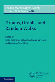
An accessible and panoramic account of the theory of random walks on groups and graphs, stressing the strong connections of the theory with other branches of mathematics, including geometric and combinatorial group theory, potential analysis, and theoretical computer science. This volume brings together original surveys and research-expository papers from renowned and leading experts, many of whom spoke at the workshop 'Groups, Graphs and Random Walks' celebrating the sixtieth birthday of Wolfgang Woess in Cortona, Italy. Topics include: growth and amenability of groups; Schrödinger operators and symbolic dynamics; ergodic theorems; Thompson's group F; Poisson boundaries; probability theory on buildings and groups of Lie type; structure trees for edge cuts in networks; and mathematical crystallography. In what is currently a fast-growing area of mathematics, this book provides an up-to-date and valuable reference for both researchers and graduate students, from which future research activities will undoubtedly stem.
By
Rostislav Grigorchuk, Mathematics Department, Texas A&M University, College Station, TX 77843-3368, USA,
Daniel Lenz, Mathematisches Institut, Friedrich Schiller Universität Jena, 07743 Jena, Germany,
Tatiana Nagnibeda, Section de Mathématiques, University of Geneva, 2-4, Rue du Lièvre, Case Postale 64, 1211 Genève 4, Suisse
By
Alexander Bendikov, Institute of Mathematics, University of Wrocław, Wrocław, Poland,
Laurent Saloff-Coste, Department of Mathematics, Cornell University, Ithaca, New York, USA