
1 Introduction
In several areas of science and industry there is a need to reliably recover a hidden multi-dimensional model parameter from noisy indirect observations. A typical example is when imaging/sensing technologies are used in medicine, engineering, astronomy and geophysics. These so-called inverse problems are often ill-posed, meaning that small errors in data may lead to large errors in the model parameter, or there are several possible model parameter values that are consistent with observations. Addressing ill-posedness is critical in applications where decision making is based on the recovered model parameter, for example in image-guided medical diagnostics. Furthermore, many highly relevant inverse problems are large-scale: they involve large amounts of data and the model parameter is high-dimensional.
Traditionally, an inverse problem is formalized as solving an equation of the form
 $$\begin{eqnarray}g={\mathcal{A}}(f)+e.\end{eqnarray}$$
Here
 $g\in Y$
is the measured data, assumed to be given, and
$g\in Y$
is the measured data, assumed to be given, and
 $f\in X$
is the model parameter we aim to reconstruct. In many applications, both
$f\in X$
is the model parameter we aim to reconstruct. In many applications, both
 $g$
and
$g$
and
 $f$
are elements in appropriate function spaces
$f$
are elements in appropriate function spaces
 $Y$
and
$Y$
and
 $X$
, respectively. The mapping
$X$
, respectively. The mapping
 ${\mathcal{A}}:X\rightarrow Y$
is the forward operator, which describes how the model parameter gives rise to data in the absence of noise and measurement errors, and
${\mathcal{A}}:X\rightarrow Y$
is the forward operator, which describes how the model parameter gives rise to data in the absence of noise and measurement errors, and
 $e\in Y$
is the observational noise that constitutes random corruptions in the data
$e\in Y$
is the observational noise that constitutes random corruptions in the data
 $g$
. The above view constitutes a knowledge-driven approach, where the forward operator and the probability distribution of the observational noise are derived from first principles.
$g$
. The above view constitutes a knowledge-driven approach, where the forward operator and the probability distribution of the observational noise are derived from first principles.
Classical research on inverse problems has focused on establishing conditions which guarantee that solutions to such ill-posed problems exist and on methods for approximating solutions in a stable way in the presence of noise (Engl, Hanke and Neubauer Reference Engl, Hanke and Neubauer2000, Benning and Burger Reference Benning and Burger2018, Louis Reference Louis1989, Kirsch Reference Kirsch2011). Despite being very successful, such a knowledge-driven approach is also associated with some shortcomings. First, the forward model is always an approximate description of reality, and extending it might be challenging due to a limited understanding of the underlying physical or technical setting. It may also be limited due to computational complexity. Accurate analytical models, such as those based on systems of non-linear partial differential equations (PDEs), may reach a numerical complexity beyond any feasible real-time potential in the foreseeable future. Second, most applications will have inputs which do not cover the full model parameter space, but stem from an unknown subset or obey an unknown stochastic distribution. The latter shortcoming in particular has led to the advance of methods that incorporate information about the structure of the parameters to be determined in terms of sparsity assumptions (Daubechies, Defrise and De Mol Reference Daubechies, Defrise and De Mol2004, Jin and Maass Reference Jin and Maass2012b ) or stochastic models (Kaipio and Somersalo Reference Kaipio and Somersalo2007, Mueller and Siltanen Reference Mueller and Siltanen2012). While representing a significant advancement in the field of inverse problems, these models are, however, limited by their inability to capture very bespoke structures in data that vary in different applications.
At the same time, data-driven approaches as they appear in machine learning offer several methods for amending such analytical models and for tackling these shortcomings. In particular, deep learning (LeCun, Bengio and Hinton Reference LeCun, Bengio and Hinton2015), which has had a transformative impact on a wide range of tasks related to artificial intelligence, ranging from computer vision and speech recognition to playing games (Igami Reference Igami2017), is starting to show its impact on inverse problems. A key feature in these methods is the use of generic models that are adapted to specific problems through learning against example data (training data). Furthermore, a common trait in the success stories for deep learning is the abundance of training data and the explicit agnosticism from a priori knowledge of how such data are generated. However, in many scientific applications, the solution method needs to be robust and there is insufficient training data to support an entirely data-driven approach. This seriously limits the use of entirely data-driven approaches for solving problems in the natural and engineering sciences, in particular for inverse problems.
A recent line of development in computational sciences combines the seemingly incompatible data- and knowledge-driven modelling paradigms. In the context of inverse problems, ideally one uses explicit knowledge-driven models when there are such available, and learns models from example data using data-driven methods only when this is necessary. Recently several algorithms have been proposed for this combination of model- and data-driven approaches for solving ill-posed inverse problems. These results are still primarily experimental and lack a thorough theoretical foundation; nevertheless, some mathematical concepts for treating data-driven approaches for inverse problems are emerging.
This survey attempts to provide an overview of methods for integrating data-driven concepts into the field of inverse problems. Particular emphasis is placed on techniques based on deep neural networks, and our aim is to pave the way for future research towards providing a solid mathematical theory. Some aspects of this development are covered in recent reviews of inverse problems and deep learning, for instance those of McCann, Jin and Unser (Reference McCann, Jin and Unser2017), Lucas, Iliadis, Molina and Katsaggelos (Reference Lucas, Iliadis, Molina and Katsaggelos2018) and McCann and Unser (Reference McCann and Unser2019).
1.1 Overview
This survey investigates algorithms for combining model- and data-driven approaches for solving inverse problems. To do so, we start by reviewing some of the main ideas of knowledge-driven approaches to inverse problems, namely functional analytic inversion (Section 2) and Bayesian inversion (Section 3), respectively. These knowledge-driven inversion techniques are derived from first principles of knowledge we have about the data, the model parameter and their relationship to each other.
Knowledge- and data-driven approaches can now be combined in several different ways depending on the type of reconstruction one seeks to compute and the type of training data. Sections 4 and 5 represent the core of the survey and discuss a range of inverse problem approaches that introduce data-driven aspects in inverse problem solutions. Here, Section 4 is the data-driven sister section to functional analytic approaches in Section 2. These approaches are primarily designed to combine data-driven methods with functional analytic inversion. This is done either to make functional analytic approaches more data-driven by appropriate parametrization of these approaches and adapting these parametrizations to data, or to accelerate an otherwise costly functional analytic reconstruction method.
Many reconstruction methods, however, are not naturally formulated within the functional analytic view of inversion. An example is the posterior mean reconstruction, whose formulation requires adopting the Bayesian view of inversion. Section 5 is the data-driven companion to Bayesian inversion in Section 3, and surveys methods that combine data- and knowledge-driven methods in Bayesian inversion. The simplest is to apply data-driven post-processing of a reconstruction obtained via a knowledge-driven method. A more sophisticated approach is to use a learned iterative scheme that integrates a knowledge-driven model for how data are generated into a data-driven method for reconstruction. The latter is done by unrolling a knowledge-driven iterative scheme, and both approaches, which compute statistical estimators, can be combined with forward operators that are partially learned via a data-driven method.
The above approaches come with different trade-offs concerning demands on training data, statistical accuracy and robustness, functional complexity, stability and interpretability. They also impact the choice of machine learning methods and algorithms for training. Certain recent – and somewhat anecdotal – topics of data-driven inverse problems are discussed in Section 6, and exemplar practical inverse problems and their data-driven solutions are presented in Section 7.
Within data-driven approaches, deep neural networks will be a focus of this survey. For an introduction to deep neural networks the reader might find it helpful to consult some introductory literature on the topic. We recommend Courville, Goodfellow and Bengio (Reference Courville, Goodfellow and Bengio2017) and Higham and Higham (Reference Higham and Higham2018) for a general introduction to deep learning; see also Vidal, Bruna, Giryes and Soatto (Reference Vidal, Bruna, Giryes and Soatto2017) for a survey of work that aims to provide a mathematical justification for several properties of deep networks. Finally, the reader may also consult Ye, Han and Cha (Reference Ye, Han and Cha2018), who give a nice survey of various types of deep neural network architectures.
Detailed structure of the paper.
In Section 2 we discuss functional analytic inversion methods, and in particular the mathematical notion of ill-posedness (Section 2.3) and regularization (Section 2.4) as a means to counteract the latter. A special focus is on variational regularization methods (Sections 2.5–2.7), as those reappear in bilevel learning in Section 4.3 in the context of data-driven methods for inverse problems.
Statistical – and in particular Bayesian – approaches to inverse problems are described in Section 3. In contrast to functional analytic approaches (Section 2.4), in Bayesian inversion (Section 3.1) the model parameter is a random variable that follows a prior distribution. A key difference between Bayesian and functional analytic inversion is that in Bayesian inversion an approximation to the whole distribution of the model parameter conditioned on the measured data (posterior distribution) is computed, rather than a single model parameter as in functional analytic inversion. This means that reconstructed model parameters can be derived via different estimates of its posterior distribution (a concept that we will encounter again in Section 5, and in particular Section 5.1.2, where data-driven reconstructions are phrased as results of different Bayes estimators), but also that uncertainty of reconstructed model parameters can be quantified (Section 3.2.5). When evaluating different reconstructions of the model parameter – which is again important when defining learning, i.e. optimization criteria for inverse problem solutions – aspects of statistical decision theory can be used (Section 3.3). Also, the parallel concept of regularization, introduced in Section 3 for the functional analytic approach, is outlined in Section 3.2 for statistical approaches. The difficult problem of selecting a prior distribution for the model parameter is discussed in Section 3.4.
In Section 4 we present some central examples of machine learning combined with functional analytic inversion. These encompass classical parameter choice rules for inverse problems (Section 4.1) and bilevel learning (Section 4.3) for parameter learning in variational regularization methods. Moreover, dictionary learning is discussed in Section 4.4 as a companion to sparse reconstruction methods in Section 2.7, but with a data-driven dictionary. Also, the concept of a black-box denoiser, and its application to inverse problems by decoupling the regularization from the inversion of the data, is presented in Section 4.6. Two recent approaches that use deep neural network parametrizations for data-driven regularization in variational inversion models are investigated in Section 4.7. In Section 4.9 we discuss a range of learned optimization methods that use data-driven approximations as a means to speed up numerical computation. Finally, in Section 4.10 we introduce a new idea of using the recently introduced concept of deep inverse priors for solving inverse problems.
In Section 5 learning data-driven inversion models are phrased in the context of statistical regularization. Section 5.1.2 connects back to the difficulty in Bayesian inversion of choosing an appropriate prior (Section 3.4), and outlines how model learning can be used to compute various Bayes estimators. Here, in particular, fully learned inversion methods (Section 5.1.3), where the whole inversion model is data-driven, are put in context with learned iterative schemes (Section 5.1.4), in which data-driven components are interwoven with inverse model assumptions. In this context also we discuss post-processing methods in Section 5.1.5, where learned regularization together with simple knowledge-driven inversion methods are used sequentially. Section 5.2 addresses the computational bottleneck of Bayesian inversion methods by using learning, and shows how one can use learning to efficiently sample from the posterior.
Section 6 covers special topics of learning in inverse problems, and in Section 6.1 includes task-based reconstruction approaches that use ideas from learned iterative reconstruction (Section 5.1.4) and deep neural networks for segmentation and classification to solve joint reconstruction-segmentation problems, learning physics-based models via neural networks (Section 6.2.1), and learning corrections to forward operators by optimization methods that perform joint reconstruction-operator correction (Section 6.2).
Finally, Section 7 illustrates some of the data-driven inversion methods discussed in the paper by applying them to practical inverse problems. These include an introductory example on inversion of ill-conditioned linear systems to highlight the intricacy of using deep learning for inverse problems as a black-box approach (Section 7.1), bilevel optimization from Section 4.3 for parameter learning in TV-type regularized problems and variational models with mixed-noise data fidelity terms (Section 7.2), the application of learned iterative reconstruction from Section 5.1.4 to computed tomography (CT) and photoacoustic tomography (PAT) (Section 7.3), adversarial regularizers from Section 4.7 for CT reconstruction as an example of variational regularization with a trained neural network as a regularizer (Section 7.4), and the application of deep inverse priors from Section 4.10 to magnetic particle imaging (MPI) (Section 7.5).
In Section 8 we finish our discussion with a few concluding remarks and comments on future research directions.
2 Functional analytic regularization
Functional analysis has had a strong impact on the development of inverse problems. One of the first publications that can be attributed to the field of inverse problems is that of Radon (Reference Radon1917). This paper derived an explicit inversion formula for the so-called Radon transform, which was later identified as a key component in the mathematical model for X-ray CT. The derivation of the inversion formula, and its analysis concerning missing stability, makes use of operator formulations that are remarkably close to the functional analysis formulations that would be developed three decades later.
2.1 The inverse problem
There is no formal mathematical definition of an inverse problem, but from an applied viewpoint such problems are concerned with determining causes from desired or observed effects. It is common to formalize this as solving an operator equation.
Definition 2.1. An inverse problem is the task of recovering the model parameter
 $f_{\text{true}}\in X$
from measured data
$f_{\text{true}}\in X$
from measured data
 $g\in Y$
, where
$g\in Y$
, where
 $$\begin{eqnarray}g={\mathcal{A}}(f_{\text{true}})+e.\end{eqnarray}$$
Here,
 $X$
(model parameter space) and
$X$
(model parameter space) and
 $Y$
(data space) are vector spaces with appropriate topologies and whose elements represent possible model parameters and data, respectively. Moreover,
$Y$
(data space) are vector spaces with appropriate topologies and whose elements represent possible model parameters and data, respectively. Moreover,
 ${\mathcal{A}}:X\rightarrow Y$
(forward operator) is a known continuous operator that maps a model parameter to data in absence of observation noise and
${\mathcal{A}}:X\rightarrow Y$
(forward operator) is a known continuous operator that maps a model parameter to data in absence of observation noise and
 $e\in Y$
is a sample of a
$e\in Y$
is a sample of a
 $Y$
-valued random variable modelling the observation noise.
$Y$
-valued random variable modelling the observation noise.
In most imaging applications, such as CT image reconstruction, elements in
 $X$
are images represented by functions defined on a fixed domain
$X$
are images represented by functions defined on a fixed domain
 $\unicode[STIX]{x1D6FA}\subset \mathbb{R}^{d}$
and elements in
$\unicode[STIX]{x1D6FA}\subset \mathbb{R}^{d}$
and elements in
 $Y$
represent imaging data by functions defined on a fixed manifold
$Y$
represent imaging data by functions defined on a fixed manifold
 $\mathbb{M}$
that is given by the acquisition geometry associated with the measurements.
$\mathbb{M}$
that is given by the acquisition geometry associated with the measurements.
2.2 Introduction to some example problems
In the following, we briefly introduce some of the key inverse problems we consider later in this survey. All are from imaging, and we make a key distinction between (i) image restoration and (ii) image reconstruction. In the former, the data are a corrupted (e.g. noisy or blurry) realization of the model parameter (image) so the reconstruction and data spaces coincide, whereas in the latter the reconstruction space is the space of images but the data space has a definition that is problem-dependent. As we will see when discussing data-driven approaches to inverse problems in Sections 4 and 5, this differentiation is particularly crucial as the difference between image and data space poses additional challenges to the design of machine learning methods. Next, we describe very briefly some of the most common operators that we will refer to below. Here the inverse problems in Sections 2.2.1–2.2.3 are image restoration problems, while those in Sections 2.2.4 and 2.2.5 are examples of image reconstruction problems.
2.2.1 Image denoising
The observed data are the ideal solution corrupted by additive noise, so the forward operator in (2.1) is the identity transform
 ${\mathcal{A}}=\text{id}$
, and we get
${\mathcal{A}}=\text{id}$
, and we get
 $$\begin{eqnarray}g=f_{\text{true}}+e,\end{eqnarray}$$
In the simplest case the distribution of the observational noise is known. Furthermore, this distribution may in more advanced problems be correlated, spatially varying and of mixed type.
In Section 7.2 we will discuss bilevel learning of total variation (TV)-type variational models for denoising of data corrupted with mixed noise distributions.
2.2.2 Image deblurring
The observed data are given by convolution with a known filter function
 $K$
together with additive noise, so (2.1) becomes
$K$
together with additive noise, so (2.1) becomes
 $$\begin{eqnarray}g=f_{\text{true}}\ast K+e.\end{eqnarray}$$
Any inverse problem of the type (2.1) with a linear forward operator that is translation-invariant will be of this form.
In the absence of noise, the inverse problem (image deconvolution) is exactly solvable by division in the Fourier domain, i.e.
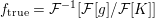 $f_{\text{true}}={\mathcal{F}}^{-1}[{\mathcal{F}}[g]/{\mathcal{F}}[K]]$
, provided that
$f_{\text{true}}={\mathcal{F}}^{-1}[{\mathcal{F}}[g]/{\mathcal{F}}[K]]$
, provided that
 ${\mathcal{F}}[K]$
has infinite support in the Fourier domain. In the presence of noise, the estimated solution is corrupted by noise whose frequency spectrum is the reciprocal of the spectrum of the filter
${\mathcal{F}}[K]$
has infinite support in the Fourier domain. In the presence of noise, the estimated solution is corrupted by noise whose frequency spectrum is the reciprocal of the spectrum of the filter
 $K$
. The distribution of the observational also has the same considerations as in (2.2). Finally, extensions include the case of a spatially varying kernel and the case where
$K$
. The distribution of the observational also has the same considerations as in (2.2). Finally, extensions include the case of a spatially varying kernel and the case where
 $K$
is unknown (blind deconvolution).
$K$
is unknown (blind deconvolution).
2.2.3 Image in-painting
Here, the observed data represents a noisy observation of the true model parameter
 $f_{\text{true}}:\unicode[STIX]{x1D6FA}\rightarrow \mathbb{R}$
restricted to a fixed measurable set
$f_{\text{true}}:\unicode[STIX]{x1D6FA}\rightarrow \mathbb{R}$
restricted to a fixed measurable set
 $\unicode[STIX]{x1D6FA}_{0}\subset \mathbb{R}^{n}$
:
$\unicode[STIX]{x1D6FA}_{0}\subset \mathbb{R}^{n}$
:
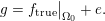 $$\begin{eqnarray}g=f_{\text{true}}\big|_{\unicode[STIX]{x1D6FA}_{0}}+e.\end{eqnarray}$$
In the above,
 $f_{\text{true}}\big|_{\unicode[STIX]{x1D6FA}_{0}}$
is the restriction of
$f_{\text{true}}\big|_{\unicode[STIX]{x1D6FA}_{0}}$
is the restriction of
 $f_{\text{true}}$
to
$f_{\text{true}}$
to
 $\unicode[STIX]{x1D6FA}_{0}$
. Solutions take different forms depending on the size of connected components in
$\unicode[STIX]{x1D6FA}_{0}$
. Solutions take different forms depending on the size of connected components in
 $\unicode[STIX]{x1D6FA}_{0}$
. Extensions include the case where
$\unicode[STIX]{x1D6FA}_{0}$
. Extensions include the case where
 $\unicode[STIX]{x1D6FA}_{0}$
is unknown or only partially known.
$\unicode[STIX]{x1D6FA}_{0}$
is unknown or only partially known.
2.2.4 Computed tomography (CT)
The simplest physical model for CT assumes mono-energetic X-rays and disregards scattering phenomena. The model parameter is then a real-valued function
 $f:\unicode[STIX]{x1D6FA}\rightarrow \mathbb{R}$
defined on a fixed domain
$f:\unicode[STIX]{x1D6FA}\rightarrow \mathbb{R}$
defined on a fixed domain
 $\unicode[STIX]{x1D6FA}\subset \mathbb{R}^{d}$
(
$\unicode[STIX]{x1D6FA}\subset \mathbb{R}^{d}$
(
 $d=2$
for two-dimensional CT and
$d=2$
for two-dimensional CT and
 $d=3$
for three-dimensional CT) that has unit mass per volume. The forward operator is the one given by the Beer–Lambert law:
$d=3$
for three-dimensional CT) that has unit mass per volume. The forward operator is the one given by the Beer–Lambert law:
 $$\begin{eqnarray}{\mathcal{A}}(f)(\unicode[STIX]{x1D714},x)=\text{e}^{-\unicode[STIX]{x1D707}\int _{-\infty }^{\infty }f(x+s\unicode[STIX]{x1D714})\,\text{d}s}.\end{eqnarray}$$
Here, the unit vector
 $\unicode[STIX]{x1D714}\in S^{d-1}$
and
$\unicode[STIX]{x1D714}\in S^{d-1}$
and
 $x\in \unicode[STIX]{x1D714}^{\bot }$
represent the line
$x\in \unicode[STIX]{x1D714}^{\bot }$
represent the line
 $\ell :s\mapsto x+s\unicode[STIX]{x1D714}$
along which the X-rays travel, and we also assume
$\ell :s\mapsto x+s\unicode[STIX]{x1D714}$
along which the X-rays travel, and we also assume
 $f$
decays fast enough for the integral to exist. In medical imaging,
$f$
decays fast enough for the integral to exist. In medical imaging,
 $\unicode[STIX]{x1D707}$
is usually set to a value that approximately corresponds to water at the X-ray energies used. The above represents pre-logarithm (or pre-log) data, and by taking the logarithm (or log) of data, one can recast the inverse problem in CT imaging to one where the forward model is the linear ray transform:
$\unicode[STIX]{x1D707}$
is usually set to a value that approximately corresponds to water at the X-ray energies used. The above represents pre-logarithm (or pre-log) data, and by taking the logarithm (or log) of data, one can recast the inverse problem in CT imaging to one where the forward model is the linear ray transform:
For low-dose imaging, pre-log data are Poisson-distributed with mean
 ${\mathcal{A}}(f_{\text{true}})$
, where
${\mathcal{A}}(f_{\text{true}})$
, where
 ${\mathcal{A}}$
is given as in (2.5), that is,
${\mathcal{A}}$
is given as in (2.5), that is,
 $g\in Y$
is a sample of
$g\in Y$
is a sample of
 $\unicode[STIX]{x1D558}\sim \operatorname{Poisson}({\mathcal{A}}(f_{\text{true}}))$
. Thus, to get rid of the non-linear exponential in (2.5), it is common to take the log of data. With such post-log data the forward operator is linear and given as in (2.6). A complication with such post-log data is that the noise model becomes non-trivial, since one takes the log of a Poisson-distributed random variable (Fu et al.
Reference Fu, Lee, Kim, Alessio, Kinahan, Chang, Sauer, Kalra and Man2017). A common approximate noise model for post-log data is (2.1), with observational noise
$\unicode[STIX]{x1D558}\sim \operatorname{Poisson}({\mathcal{A}}(f_{\text{true}}))$
. Thus, to get rid of the non-linear exponential in (2.5), it is common to take the log of data. With such post-log data the forward operator is linear and given as in (2.6). A complication with such post-log data is that the noise model becomes non-trivial, since one takes the log of a Poisson-distributed random variable (Fu et al.
Reference Fu, Lee, Kim, Alessio, Kinahan, Chang, Sauer, Kalra and Man2017). A common approximate noise model for post-log data is (2.1), with observational noise
 $e$
which is a sample of a Gaussian or Laplace-distributed random variable.
$e$
which is a sample of a Gaussian or Laplace-distributed random variable.
In the case of complete data, that is, where a full angular set of data is measured, an exact inverse is obtained by the (Fourier-transformed) data backprojected on the same lines as used for the measurements and scaled by the absolute value of the spatial frequency, followed by the inverse Fourier transform. Thus, as in deblurring, the noise is amplified, but only linearly in spatial frequency, making the problem mildly ill-posed. Extensions include the emission tomography problem (single photon emission computed tomography (SPECT) and positron emission tomography (PET)) where the line integrals are exponentially attenuated by a function
 $\unicode[STIX]{x1D707}$
that may be unknown. A major challenge in tomography is to consider incomplete data, in particular the case where only a subset of lines is measured. This problem is much more ill-posed.
$\unicode[STIX]{x1D707}$
that may be unknown. A major challenge in tomography is to consider incomplete data, in particular the case where only a subset of lines is measured. This problem is much more ill-posed.
See Sections 7.3, 7.4 and 7.6 for instances of CT reconstruction that use deep neural networks in the solution of the inverse problem.
2.2.5 Magnetic resonance imaging (MRI)
The observed data are often considered to be samples of the Fourier transform of the ideal signal, so the MRI image reconstruction problem is an inverse problem of the type (2.1), where the forward operator is given as a discrete sampling operator concatenated with the Fourier transform. A correct description of the problem takes account of the complex-valued nature of the data, which implies that when
 $e$
is normally distributed then the noise model of
$e$
is normally distributed then the noise model of
 $|{\mathcal{F}}^{-1}[g]|$
is Rician. As in CT, the case of under-sampled data is of high practical importance. In MRI, the subsampling operator has to consist of connected trajectories in Fourier space but is not restricted to straight lines.
$|{\mathcal{F}}^{-1}[g]|$
is Rician. As in CT, the case of under-sampled data is of high practical importance. In MRI, the subsampling operator has to consist of connected trajectories in Fourier space but is not restricted to straight lines.
Extensions include the case of parallel MRI where the Extensions include the case of parallel MRI where the forward operator is combined with (several) spatial sensitivity functions. More exact forward operators take account of other non-linear physical effects and can reconstruct several functions in the solution space.
2.3 Notion of ill-posedness
A difficulty in solving (2.1) is that the solution is sensitive to variations in data, which is referred to as ill-posedness. More precisely, the notion of ill-posedness is usually attributed to Hadamard, who postulated that a well-posed problem must have three defining properties, namely that (i) it has a solution (existence) that is (ii) unique and that (iii) depends continuously on the data
 $g$
(stability). Problems that do not fulfil these criteria are ill-posed and, according to Hadamard, should be modelled differently (Hadamard Reference Hadamard1902, Reference Hadamard1923).
$g$
(stability). Problems that do not fulfil these criteria are ill-posed and, according to Hadamard, should be modelled differently (Hadamard Reference Hadamard1902, Reference Hadamard1923).
For example, instability arises when the forward operator
 ${\mathcal{A}}:X\rightarrow Y$
in (2.1) has an unbounded or discontinuous inverse. Hence, every non-degenerate compact operator between infinite-dimensional Hilbert spaces whose range is infinite naturally leads to ill-posed inverse problems. Slightly more generally, one can prove that continuous operators with non-closed range yield unbounded inverses and hence lead to ill-posed inverse problems. This class includes non-degenerate compact operators as well as convolution operators on unbounded domains.
${\mathcal{A}}:X\rightarrow Y$
in (2.1) has an unbounded or discontinuous inverse. Hence, every non-degenerate compact operator between infinite-dimensional Hilbert spaces whose range is infinite naturally leads to ill-posed inverse problems. Slightly more generally, one can prove that continuous operators with non-closed range yield unbounded inverses and hence lead to ill-posed inverse problems. This class includes non-degenerate compact operators as well as convolution operators on unbounded domains.
Another way of describing ill-posedness is in terms of the set of
 $f\in X$
such that
$f\in X$
such that
 $\Vert {\mathcal{A}}(f)-g\Vert \leq \Vert e\Vert$
for given noise
$\Vert {\mathcal{A}}(f)-g\Vert \leq \Vert e\Vert$
for given noise
 $e$
in (2.1). This is an unbounded set for continuous operators with non-closed range. Finally, yet another way to understand the ill-posedness of a compact linear operator
$e$
in (2.1). This is an unbounded set for continuous operators with non-closed range. Finally, yet another way to understand the ill-posedness of a compact linear operator
 ${\mathcal{A}}$
is by means of its singular value decomposition. The decay of the spectrum
${\mathcal{A}}$
is by means of its singular value decomposition. The decay of the spectrum
 $\{{\unicode[STIX]{x1D70E}_{k}\}}_{k\in \mathbb{N}}$
is strongly related to the ill-posedness: faster decay implies a more ill-posed problem. This allows us to determine the severity of the ill-posedness. More precisely, (2.1) is weakly ill-posed if
$\{{\unicode[STIX]{x1D70E}_{k}\}}_{k\in \mathbb{N}}$
is strongly related to the ill-posedness: faster decay implies a more ill-posed problem. This allows us to determine the severity of the ill-posedness. More precisely, (2.1) is weakly ill-posed if
 $\unicode[STIX]{x1D70E}_{k}$
decays with polynomial rate as
$\unicode[STIX]{x1D70E}_{k}$
decays with polynomial rate as
 $k\rightarrow \infty$
and strongly ill-posed if the decay is exponential: see Engl et al. (Reference Engl, Hanke and Neubauer2000), Derevtsov, Efimov, Louis and Schuster (Reference Derevtsov, Efimov, Louis and Schuster2011) and Louis (Reference Louis1989) for further details. As a final note, such classification is not possible when the forward operator is non-linear. In such cases, either linearized forward operators are analysed or a non-linear spectral analysis is considered for determining the degree of ill-posedness: see e.g. Hofmann (Reference Hofmann1994). Moreover, extensions to non-compact linear operators are considered by Hofmann et al. (Reference Hofmann and Kindermann2010), for example.
$k\rightarrow \infty$
and strongly ill-posed if the decay is exponential: see Engl et al. (Reference Engl, Hanke and Neubauer2000), Derevtsov, Efimov, Louis and Schuster (Reference Derevtsov, Efimov, Louis and Schuster2011) and Louis (Reference Louis1989) for further details. As a final note, such classification is not possible when the forward operator is non-linear. In such cases, either linearized forward operators are analysed or a non-linear spectral analysis is considered for determining the degree of ill-posedness: see e.g. Hofmann (Reference Hofmann1994). Moreover, extensions to non-compact linear operators are considered by Hofmann et al. (Reference Hofmann and Kindermann2010), for example.
2.4 Regularization
Unfortunately, Hadamard’s dogma stigmatized the study of ill-posed problems and thereby severely hampered the development of the field. Mathematicians’ interest in studying ill-posed problems was revitalized by the pioneering works of Calderón and Zygmund (Reference Calderón and Zygmund1952, Reference Calderón and Zygmund1956), Calderón (Reference Calderón1958) and John (Reference John1955a , Reference John1955b , Reference John1959, Reference John1960), who showed that instability is an intrinsic property in some of the most interesting and challenging problems in mathematical physics and applied analysis. To some extent, these papers constitute the origin of the modern theory of inverse problems and regularization.
The aim of functional analytic regularization theory is to develop stable schemes for estimating
 $f_{\text{true}}$
from data
$f_{\text{true}}$
from data
 $g$
in (2.1) based on knowledge of
$g$
in (2.1) based on knowledge of
 ${\mathcal{A}}$
, and to prove analytical results for the properties of the estimated solution. More precisely, a regularization of the inverse problem in (2.1) is formally a scheme that provides a well-defined parametrized mapping
${\mathcal{A}}$
, and to prove analytical results for the properties of the estimated solution. More precisely, a regularization of the inverse problem in (2.1) is formally a scheme that provides a well-defined parametrized mapping
 ${\mathcal{R}}_{\unicode[STIX]{x1D703}}:Y\rightarrow X$
(existence) that is continuous in
${\mathcal{R}}_{\unicode[STIX]{x1D703}}:Y\rightarrow X$
(existence) that is continuous in
 $Y$
for fixed
$Y$
for fixed
 $\unicode[STIX]{x1D703}$
(stability) and convergent. The latter means there is a way to select
$\unicode[STIX]{x1D703}$
(stability) and convergent. The latter means there is a way to select
 $\unicode[STIX]{x1D703}$
so that
$\unicode[STIX]{x1D703}$
so that
 ${\mathcal{R}}_{\unicode[STIX]{x1D703}}(g)\rightarrow f_{\text{true}}$
as
${\mathcal{R}}_{\unicode[STIX]{x1D703}}(g)\rightarrow f_{\text{true}}$
as
 $g\rightarrow {\mathcal{A}}(f_{\text{true}})$
.
$g\rightarrow {\mathcal{A}}(f_{\text{true}})$
.
Besides existence, stability and convergence, a complete mathematical analysis of a regularization method also includes proving convergence rates and stability estimates. Convergence rates provide an estimate of the difference between a regularized solution
 ${\mathcal{R}}_{\unicode[STIX]{x1D703}}(g)$
and the solution of (2.1) with
${\mathcal{R}}_{\unicode[STIX]{x1D703}}(g)$
and the solution of (2.1) with
 $e=0$
(provided it exists), whereas stability estimates provide a bound on the difference between
$e=0$
(provided it exists), whereas stability estimates provide a bound on the difference between
 ${\mathcal{R}}_{\unicode[STIX]{x1D703}}(g)$
and
${\mathcal{R}}_{\unicode[STIX]{x1D703}}(g)$
and
 ${\mathcal{R}}_{\unicode[STIX]{x1D703}}({\mathcal{A}}(f_{\text{true}}))$
depending on the error
${\mathcal{R}}_{\unicode[STIX]{x1D703}}({\mathcal{A}}(f_{\text{true}}))$
depending on the error
 $\Vert e\Vert$
. These theorems rely on ‘source conditions’: for example, convergence rate results are obtained under the assumption that the true solution
$\Vert e\Vert$
. These theorems rely on ‘source conditions’: for example, convergence rate results are obtained under the assumption that the true solution
 $f_{\text{true}}$
is in the range of
$f_{\text{true}}$
is in the range of
 $[\unicode[STIX]{x2202}{\mathcal{A}}(f_{\text{true}})]^{\ast }:Y\rightarrow X$
. One difficulty is to formulate source conditions that are verifiable. This typically relates to a regularity assumption for
$[\unicode[STIX]{x2202}{\mathcal{A}}(f_{\text{true}})]^{\ast }:Y\rightarrow X$
. One difficulty is to formulate source conditions that are verifiable. This typically relates to a regularity assumption for
 $f_{\text{true}}$
that ensures a certain convergence rate: see e.g. Engl, Kunisch and Neubauer (Reference Engl, Kunisch and Neubauer1989), Hofmann, Kaltenbacher, Pöschl and Scherzer (Reference Hofmann, Kaltenbacher, Pöschl and Scherzer2007), Schuster, Kaltenbacher, Hofmann and Kazimierski (Reference Schuster, Kaltenbacher, Hofmann and Kazimierski2012), Grasmair, Haltmeier and Scherzer (Reference Grasmair, Haltmeier and Scherzer2008) and Hohage and Weidling (Reference Hohage and Weidling2016) for an example of this line of development.
$f_{\text{true}}$
that ensures a certain convergence rate: see e.g. Engl, Kunisch and Neubauer (Reference Engl, Kunisch and Neubauer1989), Hofmann, Kaltenbacher, Pöschl and Scherzer (Reference Hofmann, Kaltenbacher, Pöschl and Scherzer2007), Schuster, Kaltenbacher, Hofmann and Kazimierski (Reference Schuster, Kaltenbacher, Hofmann and Kazimierski2012), Grasmair, Haltmeier and Scherzer (Reference Grasmair, Haltmeier and Scherzer2008) and Hohage and Weidling (Reference Hohage and Weidling2016) for an example of this line of development.
From an algorithmic viewpoint, functional analytic regularization methods are subdivided into essentially four categories.
Approximate analytic inversion. These methods are based on stabilizing a closed-form expression for
 ${\mathcal{A}}^{-1}$
. This is typically achieved by considering reconstruction operators that give a mollified solution, so the resulting approaches are highly problem-specific.
${\mathcal{A}}^{-1}$
. This is typically achieved by considering reconstruction operators that give a mollified solution, so the resulting approaches are highly problem-specific.
Analytic inversion has been hugely successful: for example, filtered back projection (FBP) (Natterer Reference Natterer2001, Natterer and Wübbeling Reference Natterer and Wübbeling2001) for inverting the ray transform is still the standard method for image reconstruction in CT used in clinical practice. Furthermore, the idea of recovering a mollified version can be stated in a less problem-specific manner, which leads to the method of approximate inverse (Louis Reference Louis1996, Schuster Reference Schuster2007, Louis and Maass Reference Louis and Maass1990).
Iterative methods with early stopping. Here one typically considers iteration methods based on gradient descent for the data misfit or discrepancy term
 $f\mapsto \Vert {\mathcal{A}}(f)-g\Vert ^{2}$
. The ill-posedness of the inverse problem leads to semiconvergent behaviour, meaning that the reconstruction error decreases until a certain data fit is achieved and then starts diverging. Hence a suitable stopping needs to be designed, which acts as a regularization.
$f\mapsto \Vert {\mathcal{A}}(f)-g\Vert ^{2}$
. The ill-posedness of the inverse problem leads to semiconvergent behaviour, meaning that the reconstruction error decreases until a certain data fit is achieved and then starts diverging. Hence a suitable stopping needs to be designed, which acts as a regularization.
Well-known examples are the iterative schemes of Kaczmarz and Landweber (Engl et al. Reference Engl, Hanke and Neubauer2000, Natterer and Wübbeling Reference Natterer and Wübbeling2001, Kirsch Reference Kirsch2011). There is also large body of literature addressing iteration schemes in Krylov spaces for inverse problems (conjugate gradient (CG) type methods) as well as accelerated and discretized versions thereof (e.g. CGLS, LSQR, GMRES): see Hanke-Bourgeois (Reference Hanke-Bourgeois1995), Hanke and Hansen (Reference Hanke and Hansen1993), Frommer and Maass (Reference Frommer and Maass1999), Calvetti, Lewis and Reichel (Reference Calvetti, Lewis and Reichel2002) and Byrne (Reference Byrne2008) for further reference. A different approach that has a statistical interpretation uses a fixed-point iteration for the maximum a posteriori (MAP) estimator leading to the maximum likelihood expectationmaximization (ML-EM) algorithm (Dempster et al. Reference Dempster, Laird and Rubin1977).
Discretization as regularization. Projection or Galerkin methods, which search for an approximate solution of an inverse problems in a predefined subspace, are also a powerful tool for solving inverse problems. The level of discretization controls the approximation of the forward operator but it also stabilizes the inversion process: see Engl et al. (Reference Engl, Hanke and Neubauer2000), Plato and Vainikko (Reference Plato and Vainikko1990) and Natterer (Reference Natterer1977). Such concepts have been discussed in the framework of parameter identification for partial differential equations (quasi-reversibility): see Lattès and Lions (Reference Lattès and Lions1969) for an early reference and Hämarik, Kaltenbacher, Kangro and Resmerita (Reference Hämarik, Kaltenbacher, Kangro and Resmerita2016) and Kaltenbacher, Kirchner and Vexler (Reference Kaltenbacher, Kirchner and Vexler2011) for some recent developments.
Variational methods. The idea here is to minimize a measure of data misfit that is penalized using a regularizer (Kaltenbacher, Neubauer and Scherzer Reference Kaltenbacher, Neubauer and Scherzer2008, Scherzer et al. Reference Scherzer, Grasmair, Grossauer, Haltmeier and Lenzen2009):
where we make use of the notation in Definitions 2.2, 2.4 and 2.5. This is a generic, yet highly adaptable, framework for reconstruction with a natural plug-and-play structure where the forward operator
 ${\mathcal{A}}$
, the data discrepancy
${\mathcal{A}}$
, the data discrepancy
 ${\mathcal{L}}$
and the regularizer
${\mathcal{L}}$
and the regularizer
 ${\mathcal{S}}_{\unicode[STIX]{x1D703}}$
are chosen to fit the specific aspects of the inverse problem. Well-known examples are classical Tikhonov regularization and TV regularization.
${\mathcal{S}}_{\unicode[STIX]{x1D703}}$
are chosen to fit the specific aspects of the inverse problem. Well-known examples are classical Tikhonov regularization and TV regularization.
Sections 2.5 and 2.6 provide a closer look at the development of variational methods since these play an important role in Section 4, where data-driven methods are used in functional analytic regularization. To simplify these descriptions it is convenient to establish some key notions.
Definition 2.2. A regularization functional
 ${\mathcal{S}}:X\rightarrow \mathbb{R}_{+}$
quantifies how well a model parameter possesses desirable features: a larger value usually means less desirable properties.
${\mathcal{S}}:X\rightarrow \mathbb{R}_{+}$
quantifies how well a model parameter possesses desirable features: a larger value usually means less desirable properties.
In variational approaches to inverse problems, the value of
 ${\mathcal{S}}$
is considered as a penalty term, and in Bayesian approaches it is seen as the negative log of a prior probability distribution. Henceforth we will use
${\mathcal{S}}$
is considered as a penalty term, and in Bayesian approaches it is seen as the negative log of a prior probability distribution. Henceforth we will use
 ${\mathcal{S}}_{\unicode[STIX]{x1D703}}$
to denote a regularization term that depends on a parameter set
${\mathcal{S}}_{\unicode[STIX]{x1D703}}$
to denote a regularization term that depends on a parameter set
 $\unicode[STIX]{x1D703}\in \unicode[STIX]{x1D6E9}$
; in particular we will use
$\unicode[STIX]{x1D703}\in \unicode[STIX]{x1D6E9}$
; in particular we will use
 $\unicode[STIX]{x1D703}$
as parameters that will be learned.
$\unicode[STIX]{x1D703}$
as parameters that will be learned.
Remark 2.3. In some cases
 $\unicode[STIX]{x1D703}$
is a single scalar. We will use the notation
$\unicode[STIX]{x1D703}$
is a single scalar. We will use the notation
 $\unicode[STIX]{x1D706}{\mathcal{S}}(f)\equiv {\mathcal{S}}_{\unicode[STIX]{x1D703}}(f)$
wherever such usage is unambiguous, and with the implication that
$\unicode[STIX]{x1D706}{\mathcal{S}}(f)\equiv {\mathcal{S}}_{\unicode[STIX]{x1D703}}(f)$
wherever such usage is unambiguous, and with the implication that
 $\unicode[STIX]{x1D703}=\unicode[STIX]{x1D706}\in \mathbb{R}_{+}$
. Furthermore, we will sometimes express the set
$\unicode[STIX]{x1D703}=\unicode[STIX]{x1D706}\in \mathbb{R}_{+}$
. Furthermore, we will sometimes express the set
 $\unicode[STIX]{x1D703}$
explicitly, e.g.
$\unicode[STIX]{x1D703}$
explicitly, e.g.
 ${\mathcal{S}}_{\unicode[STIX]{x1D6FC},\unicode[STIX]{x1D6FD}}$
, where the usage is unambiguous.
${\mathcal{S}}_{\unicode[STIX]{x1D6FC},\unicode[STIX]{x1D6FD}}$
, where the usage is unambiguous.
Definition 2.4. A data discrepancy functional
 ${\mathcal{L}}:Y\times Y\rightarrow \mathbb{R}$
is a scalar quantification of the similarity between two elements of data space
${\mathcal{L}}:Y\times Y\rightarrow \mathbb{R}$
is a scalar quantification of the similarity between two elements of data space
 $Y$
.
$Y$
.
The data discrepancy functional is considered to be a data fitting term in variational approaches to inverse problems. Although often taken to be a metric on data space, choosing it as an affine transformation of the negative log-likelihood of data allows for a statistical interpretation, since minimizing
 $f\mapsto {\mathcal{L}}({\mathcal{A}}(f),g)$
amounts to finding a maximum likelihood solution. For Gaussian observational noise
$f\mapsto {\mathcal{L}}({\mathcal{A}}(f),g)$
amounts to finding a maximum likelihood solution. For Gaussian observational noise
 $\unicode[STIX]{x1D556}\sim \operatorname{N}(0,\unicode[STIX]{x1D6E4})$
, the corresponding data discrepancy is then given by the Mahalanobis distance:
$\unicode[STIX]{x1D556}\sim \operatorname{N}(0,\unicode[STIX]{x1D6E4})$
, the corresponding data discrepancy is then given by the Mahalanobis distance:
 $$\begin{eqnarray}{\mathcal{L}}(g,v) :=\Vert g-v\Vert _{\unicode[STIX]{x1D6E4}^{-1}}^{2}\quad \text{for }g,v\in Y.\end{eqnarray}$$
If data are Poisson-distributed, i.e.
 $\unicode[STIX]{x1D558}\sim \operatorname{Poisson}({\mathcal{A}}(f_{\text{true}}))$
, then an appropriate data discrepancy functional is the Kullback–Leibler (KL) divergence. When elements in data space
$\unicode[STIX]{x1D558}\sim \operatorname{Poisson}({\mathcal{A}}(f_{\text{true}}))$
, then an appropriate data discrepancy functional is the Kullback–Leibler (KL) divergence. When elements in data space
 $Y$
are real-valued functions on
$Y$
are real-valued functions on
 $\mathbb{M}$
, then the KL divergence becomes
$\mathbb{M}$
, then the KL divergence becomes
Similarly, Laplace-distributed observational noise corresponds to a data discrepancy that is given by the 1-norm. One can also express the data log-likelihood for Poisson-distributed data with an additive observational noise term that is Gaussian, but the resulting expressions are quite complex (Benvenuto et al. Reference Benvenuto, Camera, Theys, Ferrari, Lantéri and Bertero2008).
Definition 2.5. A reconstruction operator
 ${\mathcal{R}}:Y\rightarrow X$
is a mapping which gives a point estimate
${\mathcal{R}}:Y\rightarrow X$
is a mapping which gives a point estimate
 $\hat{f}$
as the solution to (2.1).
$\hat{f}$
as the solution to (2.1).
Henceforth we will use
 ${\mathcal{R}}_{\unicode[STIX]{x1D703}}$
to denote a reconstruction operator that depends on a parameter set
${\mathcal{R}}_{\unicode[STIX]{x1D703}}$
to denote a reconstruction operator that depends on a parameter set
 $\unicode[STIX]{x1D703}\in \unicode[STIX]{x1D6E9}$
; in particular we will use
$\unicode[STIX]{x1D703}\in \unicode[STIX]{x1D6E9}$
; in particular we will use
 $\unicode[STIX]{x1D703}$
as parameters that will be learned.
$\unicode[STIX]{x1D703}$
as parameters that will be learned.
Remark 2.6. In variational approaches we will typically use the notation
 ${\mathcal{R}}_{\unicode[STIX]{x1D706}}$
to denote an operator parametrized by a single scalar
${\mathcal{R}}_{\unicode[STIX]{x1D706}}$
to denote an operator parametrized by a single scalar
 $\unicode[STIX]{x1D706}>0$
which corresponds (explicitly or implicitly) to optimizing a functional that includes a regularization penalty
$\unicode[STIX]{x1D706}>0$
which corresponds (explicitly or implicitly) to optimizing a functional that includes a regularization penalty
 $\unicode[STIX]{x1D706}{\mathcal{S}}$
as in Definition 2.2. More generally
$\unicode[STIX]{x1D706}{\mathcal{S}}$
as in Definition 2.2. More generally
 $\unicode[STIX]{x1D703}$
will also be used to define the parameters of an algorithm or neural network used to generate a solution
$\unicode[STIX]{x1D703}$
will also be used to define the parameters of an algorithm or neural network used to generate a solution
 $f_{\unicode[STIX]{x1D703}}$
that may or may not explicitly specify a regularization functional. Again we will assume the context provides an unambiguous justification for the choice between
$f_{\unicode[STIX]{x1D703}}$
that may or may not explicitly specify a regularization functional. Again we will assume the context provides an unambiguous justification for the choice between
 ${\mathcal{R}}_{\unicode[STIX]{x1D703}}$
and
${\mathcal{R}}_{\unicode[STIX]{x1D703}}$
and
 ${\mathcal{R}}_{\unicode[STIX]{x1D706}}$
. Furthermore, we will sometimes express the set
${\mathcal{R}}_{\unicode[STIX]{x1D706}}$
. Furthermore, we will sometimes express the set
 $\unicode[STIX]{x1D703}$
explicitly, e.g.
$\unicode[STIX]{x1D703}$
explicitly, e.g.
 ${\mathcal{R}}_{{\mathcal{W}},\unicode[STIX]{x1D713}}$
, where the usage is unambiguous.
${\mathcal{R}}_{{\mathcal{W}},\unicode[STIX]{x1D713}}$
, where the usage is unambiguous.
2.5 Classical Tikhonov regularization
Tikhonov (or Tikhonov–Phillips) regularization is arguably the most prominent technique for inverse problems. It was introduced by Tikhonov (Reference Tikhonov1943, Reference Tikhonov1963), Phillips (Reference Phillips1962) and Tikhonov and Arsenin (Reference Tikhonov and Arsenin1977) for solving ill-posed inverse problems of the form (2.1), and can be stated in the form
Bearing in mind the notation in Remarks 2.3 and 2.6, note that (2.10) has the form of (2.7) with
 ${\mathcal{L}}$
given by the squared
${\mathcal{L}}$
given by the squared
 $L^{2}$
-distance. Here
$L^{2}$
-distance. Here
 $X$
and
$X$
and
 $Y$
are Hilbert spaces (typically both are
$Y$
are Hilbert spaces (typically both are
 $L^{2}$
spaces). Moreover, the choice
$L^{2}$
spaces). Moreover, the choice
 ${\mathcal{S}}(f):=\frac{1}{2}\Vert f\Vert ^{2}$
is the most common one for the penalty term in (2.10). In fact, if
${\mathcal{S}}(f):=\frac{1}{2}\Vert f\Vert ^{2}$
is the most common one for the penalty term in (2.10). In fact, if
 ${\mathcal{A}}$
is linear, with
${\mathcal{A}}$
is linear, with
 ${\mathcal{A}}^{\ast }$
denoting its adjoint, then standard arguments for minimizing quadratic functionals yield
${\mathcal{A}}^{\ast }$
denoting its adjoint, then standard arguments for minimizing quadratic functionals yield
 $$\begin{eqnarray}{\mathcal{R}}_{\unicode[STIX]{x1D706}}=({\mathcal{A}}^{\ast }\circ {\mathcal{A}}+\unicode[STIX]{x1D706}\text{id})^{-1}\circ {\mathcal{A}}^{\ast }.\end{eqnarray}$$
Until the late 1980s the analytical investigations of regularization schemes of the type in (2.10) were restricted either to linear operators or to rather specific approaches for selected non-linear problems. Many inverse problems, such as parameter identification in linear differential operators, lead to non-linear parameter-to-state maps, so the corresponding forward operator becomes non-linear (Arridge and Schotland Reference Arridge and Schotland2009, Greenleaf, Kurylev, Lassas and Uhlmann Reference Greenleaf, Kurylev, Lassas and Uhlmann2007, Bal, Chung and Schotland Reference Bal, Chung and Schotland2016, Jin and Maass Reference Jin and Maass2012b , Jin and Maass Reference Jin and Maass2012a ).
Analysis of (2.10) for non-linear forward operators is difficult, for example, singular value decompositions are not available. A major theoretical breakthrough came with the publications of Seidman and Vogel (Reference Seidman and Vogel1989) and Engl et al. (Reference Engl, Kunisch and Neubauer1989), which extended the theoretical investigation of Tikhonov regularization to the non-linear setting by introducing radically new concepts. Among others, it extended the notion of minimum norm solution used in theorems dealing with convergence rates to
 $f_{0}$
-minimum norm solutions. This means one assumes the knowledge of some meaningful parameter
$f_{0}$
-minimum norm solutions. This means one assumes the knowledge of some meaningful parameter
 $f_{0}\in X$
and the aim of the regularization method is to approximate a solution that in the limit minimizes
$f_{0}\in X$
and the aim of the regularization method is to approximate a solution that in the limit minimizes
 $\Vert f-f_{0}\Vert$
amongst all solutions of
$\Vert f-f_{0}\Vert$
amongst all solutions of
 ${\mathcal{A}}(f)=g$
. Hence,
${\mathcal{A}}(f)=g$
. Hence,
 $f_{0}$
acts as a kind of prior. Among the main results of Engl et al. (Reference Engl, Kunisch and Neubauer1989) is a theorem that estimates the convergence rate assuming sufficient regularity of the forward operator
$f_{0}$
acts as a kind of prior. Among the main results of Engl et al. (Reference Engl, Kunisch and Neubauer1989) is a theorem that estimates the convergence rate assuming sufficient regularity of the forward operator
 ${\mathcal{A}}$
and a source condition that relates the penalty term to the functional
${\mathcal{A}}$
and a source condition that relates the penalty term to the functional
 ${\mathcal{A}}$
at
${\mathcal{A}}$
at
 $f_{\text{true}}$
. This theorem, which is stated below, opened the path to many successful applications, particularly for parameter identification problems related to partial differential equations, and such assumptions occur in different variations in all theorems related to the variational approach.
$f_{\text{true}}$
. This theorem, which is stated below, opened the path to many successful applications, particularly for parameter identification problems related to partial differential equations, and such assumptions occur in different variations in all theorems related to the variational approach.
Theorem 2.7. Consider the inverse problem in (2.1) where
 ${\mathcal{A}}:X\rightarrow Y$
is continuous, weakly sequentially closed and with a convex domain. Next, assume there exists a
${\mathcal{A}}:X\rightarrow Y$
is continuous, weakly sequentially closed and with a convex domain. Next, assume there exists a
 $f_{0}$
-minimum norm solution
$f_{0}$
-minimum norm solution
 $f_{\text{true}}$
for some fixed
$f_{\text{true}}$
for some fixed
 $f_{0}\in X$
and let data
$f_{0}\in X$
and let data
 $g\in Y$
in (2.1) satisfy
$g\in Y$
in (2.1) satisfy
 $\Vert {\mathcal{A}}(f_{\text{true}})-g\Vert \leq \unicode[STIX]{x1D6FF}$
. Also, let
$\Vert {\mathcal{A}}(f_{\text{true}})-g\Vert \leq \unicode[STIX]{x1D6FF}$
. Also, let
 $f_{\unicode[STIX]{x1D706}}^{\unicode[STIX]{x1D6FF}}\in X$
denote a minimizer of (2.10) with
$f_{\unicode[STIX]{x1D706}}^{\unicode[STIX]{x1D6FF}}\in X$
denote a minimizer of (2.10) with
 ${\mathcal{S}}(f) :=\frac{1}{2}\Vert f\Vert ^{2}$
. Finally, assume the following.
${\mathcal{S}}(f) :=\frac{1}{2}\Vert f\Vert ^{2}$
. Finally, assume the following.
(1)
 ${\mathcal{A}}$
has a continuous Fréchet derivative.
${\mathcal{A}}$
has a continuous Fréchet derivative.(2) There exists a
$\unicode[STIX]{x1D6FE}>0$
, such that for all$$\begin{eqnarray}\Vert [\unicode[STIX]{x2202}\!{\mathcal{A}}(f_{\text{true}})]-[\unicode[STIX]{x2202}\!{\mathcal{A}}(f)]\Vert _{L(X,Y)}\leq \unicode[STIX]{x1D6FE}\Vert f_{\text{true}}-f\Vert _{X}\end{eqnarray}$$
$f\in \operatorname{dom}({\mathcal{A}})\cap B_{r}(f_{\text{true}})$
with
$r>2\Vert f_{\text{true}}-f_{0}\Vert$
. Here,
$L(X,Y)$
is the vector space of
$Y$
-valued linear maps on
$X$
and
$B_{r}(f_{\text{true}})\subset X$
denotes a ball of radius
$r$
around
$f_{\text{true}}$
.(3) There exists
$v\in Y$
with
$\unicode[STIX]{x1D6FE}\Vert v\Vert <1$
such that
$f_{\text{true}}-f_{0}=[\unicode[STIX]{x2202}\!{\mathcal{A}}(f_{\text{true}})]^{\ast }(v)$
.


Then, choosing
 $\unicode[STIX]{x1D706}\propto \unicode[STIX]{x1D6FF}$
as
$\unicode[STIX]{x1D706}\propto \unicode[STIX]{x1D6FF}$
as
 $\unicode[STIX]{x1D6FF}\rightarrow 0$
yields
$\unicode[STIX]{x1D6FF}\rightarrow 0$
yields
 $$\begin{eqnarray}\Vert f_{\unicode[STIX]{x1D706}}^{\unicode[STIX]{x1D6FF}}-f_{\text{true}}\Vert =O(\sqrt{\unicode[STIX]{x1D6FF}})\quad \text{and}\quad \Vert {\mathcal{A}}(f_{\unicode[STIX]{x1D706}}^{\unicode[STIX]{x1D6FF}})-g\Vert =O(\unicode[STIX]{x1D6FF}).\end{eqnarray}$$
2.6 Extension of classical Tikhonov regularization
Tikhonov regularization is a particular case of the more general variational regularization schemes (2.7). In fact, penalty terms for Tikhonov-type functionals, as well as suitable source conditions, have been generalized considerably in a series of papers. A key issue in solving an inverse problem is to use a forward operator
 ${\mathcal{A}}$
that is sufficiently accurate. It is also important to choose an appropriate data discrepancy
${\mathcal{A}}$
that is sufficiently accurate. It is also important to choose an appropriate data discrepancy
 ${\mathcal{L}}$
, regularizer
${\mathcal{L}}$
, regularizer
 ${\mathcal{S}}_{\unicode[STIX]{x1D703}}$
, and to have a parameter choice rule for setting
${\mathcal{S}}_{\unicode[STIX]{x1D703}}$
, and to have a parameter choice rule for setting
 $\unicode[STIX]{x1D703}$
. Depending on these choices, different reconstruction results are obtained.
$\unicode[STIX]{x1D703}$
. Depending on these choices, different reconstruction results are obtained.
The data discrepancy.
Here the choice is ideally guided by statistical considerations for the observation noise (Bertero, Lantéri and Zanni Reference Bertero, Lantéri, Zanni and Censor2008). Ideally one selects
 ${\mathcal{L}}$
as an appropriate affine transform of the negative log-likelihood of data, in which case minimizing
${\mathcal{L}}$
as an appropriate affine transform of the negative log-likelihood of data, in which case minimizing
 $f\mapsto {\mathcal{L}}({\mathcal{A}}(f),g)$
becomes the same as computing an maximum likelihood estimator. Hence, Poisson-distributed data that typically appear in photography (Costantini and Susstrunk Reference Costantini and Susstrunk2004) and emission tomography applications (Vardi, Shepp and Kaufman Reference Vardi, Shepp and Kaufman1985) lead to a data discrepancy given by the Kullback–Leibler divergence (Sawatzky, Brune, Müller and Burger Reference Sawatzky, Brune, Müller, Burger, Jiang and Petkov2009, Hohage and Werner Reference Hohage and Werner2016), while additive normally distributed data, as for Gaussian noise, result in a least-squares fit model.
$f\mapsto {\mathcal{L}}({\mathcal{A}}(f),g)$
becomes the same as computing an maximum likelihood estimator. Hence, Poisson-distributed data that typically appear in photography (Costantini and Susstrunk Reference Costantini and Susstrunk2004) and emission tomography applications (Vardi, Shepp and Kaufman Reference Vardi, Shepp and Kaufman1985) lead to a data discrepancy given by the Kullback–Leibler divergence (Sawatzky, Brune, Müller and Burger Reference Sawatzky, Brune, Müller, Burger, Jiang and Petkov2009, Hohage and Werner Reference Hohage and Werner2016), while additive normally distributed data, as for Gaussian noise, result in a least-squares fit model.
The regularizer.
As stated in Definition 2.2,
 ${\mathcal{S}}$
acts as a penalizer and is chosen to enforce stability by encoding a priori information about
${\mathcal{S}}$
acts as a penalizer and is chosen to enforce stability by encoding a priori information about
 $f_{\text{true}}$
. How to set the (regularization) parameter
$f_{\text{true}}$
. How to set the (regularization) parameter
 $\unicode[STIX]{x1D703}$
reflects noise level in data: see Section 4.1.
$\unicode[STIX]{x1D703}$
reflects noise level in data: see Section 4.1.
Classical Tikhonov regularization (2.10) uses Hilbert-space norms (or semi-norms) to regularize the inverse problems. In more recent years, Banach-space regularizers have become more popular in the context of sparsity-promoting and discontinuity-preserving regularization, which are revisited in Section 2.7. TV regularization was introduced by Rudin, Osher and Fatemi (Reference Rudin, Osher and Fatemi1992) for image denoising due to its edge-preserving properties, favouring images
 $f$
that have a sparse gradient. Here, the TV regularizer is given as
$f$
that have a sparse gradient. Here, the TV regularizer is given as
where
 $\unicode[STIX]{x1D6FA}\subset \mathbb{R}^{d}$
is a fixed open and bounded set. The above functional (TV regularizer) uses the total variation measure of the distributional derivative of
$\unicode[STIX]{x1D6FA}\subset \mathbb{R}^{d}$
is a fixed open and bounded set. The above functional (TV regularizer) uses the total variation measure of the distributional derivative of
 $f$
defined on
$f$
defined on
 $\unicode[STIX]{x1D6FA}$
(Ambrosio, Fusco and Pallara Reference Ambrosio, Fusco and Pallara2000). A drawback of using such a regularization procedure is apparent as soon as the true model parameter not only consists of constant regions and jumps but also possesses more complicated, higher-order structures, e.g. piecewise linear parts. In this case, TV introduces jumps that are not present in the true solution, which is referred to as staircasing (Ring Reference Ring2000). Examples of generalizations of TV for addressing this drawback typically incorporate higher-order derivatives, e.g. total generalized variation (TGV) (Bredies, Kunisch and Pock Reference Bredies, Kunisch and Pock2011) and the infimal-convolution total variation (ICTV) model (Chambolle and Lions Reference Chambolle and Lions1997). These read as
$\unicode[STIX]{x1D6FA}$
(Ambrosio, Fusco and Pallara Reference Ambrosio, Fusco and Pallara2000). A drawback of using such a regularization procedure is apparent as soon as the true model parameter not only consists of constant regions and jumps but also possesses more complicated, higher-order structures, e.g. piecewise linear parts. In this case, TV introduces jumps that are not present in the true solution, which is referred to as staircasing (Ring Reference Ring2000). Examples of generalizations of TV for addressing this drawback typically incorporate higher-order derivatives, e.g. total generalized variation (TGV) (Bredies, Kunisch and Pock Reference Bredies, Kunisch and Pock2011) and the infimal-convolution total variation (ICTV) model (Chambolle and Lions Reference Chambolle and Lions1997). These read as
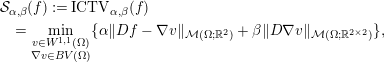 $$\begin{eqnarray}\displaystyle & & \displaystyle {\mathcal{S}}_{\unicode[STIX]{x1D6FC},\unicode[STIX]{x1D6FD}}(f) :=\operatorname{ICTV}_{\unicode[STIX]{x1D6FC},\unicode[STIX]{x1D6FD}}(f)\nonumber\\ \displaystyle & & \displaystyle \quad =\min _{\substack{ v\in W^{1,1}(\unicode[STIX]{x1D6FA}) \\ \unicode[STIX]{x1D6FB}v\in BV(\unicode[STIX]{x1D6FA})}}\{\unicode[STIX]{x1D6FC}\Vert Df-\unicode[STIX]{x1D6FB}v\Vert _{{\mathcal{M}}(\unicode[STIX]{x1D6FA};\mathbb{R}^{2})}+\unicode[STIX]{x1D6FD}\Vert D\unicode[STIX]{x1D6FB}v\Vert _{{\mathcal{M}}(\unicode[STIX]{x1D6FA};\mathbb{R}^{2\times 2})}\},\end{eqnarray}$$
and the second-order TGV (Bredies and Valkonen Reference Bredies and Valkonen2011, Bredies, Kunisch and Valkonen Reference Bredies, Kunisch and Valkonen2013) reads as
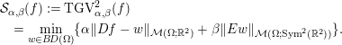 $$\begin{eqnarray}\displaystyle & & \displaystyle {\mathcal{S}}_{\unicode[STIX]{x1D6FC},\unicode[STIX]{x1D6FD}}(f) :=\operatorname{TGV}_{\unicode[STIX]{x1D6FC},\unicode[STIX]{x1D6FD}}^{2}(f)\nonumber\\ \displaystyle & & \displaystyle \quad =\min _{w\in B\!D(\unicode[STIX]{x1D6FA})}\{\unicode[STIX]{x1D6FC}\Vert Df-w\Vert _{{\mathcal{M}}(\unicode[STIX]{x1D6FA};\mathbb{R}^{2})}+\unicode[STIX]{x1D6FD}\Vert Ew\Vert _{{\mathcal{M}}(\unicode[STIX]{x1D6FA};\operatorname{Sym}^{2}(\mathbb{R}^{2}))}\}.\end{eqnarray}$$
Here
 $$\begin{eqnarray}B\!D(\unicode[STIX]{x1D6FA}) :=\{w\in L^{1}(\unicode[STIX]{x1D6FA};\mathbb{R}^{d})\mid \Vert Ew\Vert _{{\mathcal{M}}(\unicode[STIX]{x1D6FA};\mathbb{R}^{d\times d})}<\infty \}\end{eqnarray}$$
is the space of vector fields of bounded deformation on
 $\unicode[STIX]{x1D6FA}$
with
$\unicode[STIX]{x1D6FA}$
with
 $E$
denoting the symmetrized gradient and
$E$
denoting the symmetrized gradient and
 $\text{Sym}^{2}(\mathbb{R}^{2})$
the space of symmetric tensors of order
$\text{Sym}^{2}(\mathbb{R}^{2})$
the space of symmetric tensors of order
 $2$
with arguments in
$2$
with arguments in
 $\mathbb{R}^{2}$
. The parameters
$\mathbb{R}^{2}$
. The parameters
 $\unicode[STIX]{x1D6FC},\unicode[STIX]{x1D6FD}$
are fixed positive parameters. The main difference between (2.13) and (2.14) is that we do not generally have
$\unicode[STIX]{x1D6FC},\unicode[STIX]{x1D6FD}$
are fixed positive parameters. The main difference between (2.13) and (2.14) is that we do not generally have
 $w=\unicode[STIX]{x1D6FB}v$
for any function
$w=\unicode[STIX]{x1D6FB}v$
for any function
 $v$
. That results in some qualitative differences of ICTV and TGV regularization: see e.g. Benning, Brune, Burger and Müller (Reference Benning, Brune, Burger and Müller2013). One may also consider Banach-space norms other than TV, such as Besov norms (Lassas, Saksman and Siltanen Reference Lassas, Saksman and Siltanen2009), which behave more nicely with respect to discretization (see also Section 3.4). Different TV-type regularizers and their adaption to data by bilevel learning of parameters (e.g.
$v$
. That results in some qualitative differences of ICTV and TGV regularization: see e.g. Benning, Brune, Burger and Müller (Reference Benning, Brune, Burger and Müller2013). One may also consider Banach-space norms other than TV, such as Besov norms (Lassas, Saksman and Siltanen Reference Lassas, Saksman and Siltanen2009), which behave more nicely with respect to discretization (see also Section 3.4). Different TV-type regularizers and their adaption to data by bilevel learning of parameters (e.g.
 $\unicode[STIX]{x1D6FC}$
and
$\unicode[STIX]{x1D6FC}$
and
 $\unicode[STIX]{x1D6FD}$
in ICTV and TGV) will be discussed in more detail in Section 4.3.1 and numerical results will be given in Section 7.2.
$\unicode[STIX]{x1D6FD}$
in ICTV and TGV) will be discussed in more detail in Section 4.3.1 and numerical results will be given in Section 7.2.
Finally, in applied harmonic analysis,
 $\ell _{p}$
-norms of wavelets have been proposed as regularizers (Daubechies et al.
Reference Daubechies1991, Mallat Reference Mallat2009, Unser and Blu Reference Unser and Blu2000, Kutyniok and Labate Reference Kutyniok and Labate2012, Eldar and Kutyniok Reference Eldar and Kutyniok2012, Foucart and Rauhut Reference Foucart and Rauhut2013). Other examples are non-local regularization (Gilboa and Osher Reference Gilboa and Osher2008, Buades, Coll and Morel Reference Buades, Coll and Morel2005), anisotropic regularizers (Weickert Reference Weickert1998) and, in the context of free discontinuity problems, the representation of images as a composition of smooth parts separated by edges (Blake and Zisserman Reference Blake and Zisserman1987, Mumford and Shah Reference Mumford and Shah1989, Carriero, Leaci and Tomarelli Reference Carriero, Leaci, Tomarelli, Serapioni and Tomarelli1996).
$\ell _{p}$
-norms of wavelets have been proposed as regularizers (Daubechies et al.
Reference Daubechies1991, Mallat Reference Mallat2009, Unser and Blu Reference Unser and Blu2000, Kutyniok and Labate Reference Kutyniok and Labate2012, Eldar and Kutyniok Reference Eldar and Kutyniok2012, Foucart and Rauhut Reference Foucart and Rauhut2013). Other examples are non-local regularization (Gilboa and Osher Reference Gilboa and Osher2008, Buades, Coll and Morel Reference Buades, Coll and Morel2005), anisotropic regularizers (Weickert Reference Weickert1998) and, in the context of free discontinuity problems, the representation of images as a composition of smooth parts separated by edges (Blake and Zisserman Reference Blake and Zisserman1987, Mumford and Shah Reference Mumford and Shah1989, Carriero, Leaci and Tomarelli Reference Carriero, Leaci, Tomarelli, Serapioni and Tomarelli1996).
2.7 Sparsity-promoting regularization
Sparsity is an important concept in conceiving inversion models as well as learning parts of them. In what follows we review some of the main approaches to computing sparse solutions, and postpone learning sparse representations to Section 4.4.
2.7.1 Notions of sparsity
Let
 $X$
be a separable Hilbert space, that is, we will assume that it has a countable orthonormal basis. A popular approach to sparse reconstruction uses the notion of a dictionary
$X$
be a separable Hilbert space, that is, we will assume that it has a countable orthonormal basis. A popular approach to sparse reconstruction uses the notion of a dictionary
 $\mathbb{D} :=\{\unicode[STIX]{x1D719}_{i}\}\subset X$
, whose elements are called atoms. Here,
$\mathbb{D} :=\{\unicode[STIX]{x1D719}_{i}\}\subset X$
, whose elements are called atoms. Here,
 $\mathbb{D}$
is either given, i.e. knowledge-driven, or data-driven and derived from a set of realizations
$\mathbb{D}$
is either given, i.e. knowledge-driven, or data-driven and derived from a set of realizations
 $f_{i}\in X$
: see Bruckstein, Donoho and Elad (Reference Bruckstein, Donoho and Elad2009), Daubechies et al. (Reference Daubechies, Defrise and De Mol2004), Rubinstein, Bruckstein and Elad (Reference Rubinstein, Bruckstein and Elad.2010), Lanusse, Starck, Woiselle and Fadili (Reference Lanusse, Starck, Woiselle and Fadili2014) and Chen and Needell (Reference Chen and Needell2016).
$f_{i}\in X$
: see Bruckstein, Donoho and Elad (Reference Bruckstein, Donoho and Elad2009), Daubechies et al. (Reference Daubechies, Defrise and De Mol2004), Rubinstein, Bruckstein and Elad (Reference Rubinstein, Bruckstein and Elad.2010), Lanusse, Starck, Woiselle and Fadili (Reference Lanusse, Starck, Woiselle and Fadili2014) and Chen and Needell (Reference Chen and Needell2016).
A special class of dictionaries is that of frames. A dictionary
 $\mathbb{D} :=\{\unicode[STIX]{x1D719}_{i}\}$
is a frame if there exists
$\mathbb{D} :=\{\unicode[STIX]{x1D719}_{i}\}$
is a frame if there exists
 $C_{1},C_{2}>0$
such that
$C_{1},C_{2}>0$
such that
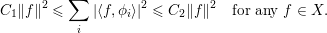 $$\begin{eqnarray}C_{1}\Vert f\Vert ^{2}\leq \mathop{\sum }_{i}|\langle f,\unicode[STIX]{x1D719}_{i}\rangle |^{2}\leq C_{2}\Vert f\Vert ^{2}\quad \text{for any }f\in X.\end{eqnarray}$$
A frame is called tight if
 $C_{1}=C_{2}=1$
; it is called over-complete or redundant if
$C_{1}=C_{2}=1$
; it is called over-complete or redundant if
 $\mathbb{D}$
does not form a basis for
$\mathbb{D}$
does not form a basis for
 $X$
. Redundant dictionaries, e.g. translation-invariant wavelets, often work better than non-redundant dictionaries: see Peyré, Bougleux and Cohen (Reference Peyré, Bougleux and Cohen2011) and Elad (Reference Elad2010).
$X$
. Redundant dictionaries, e.g. translation-invariant wavelets, often work better than non-redundant dictionaries: see Peyré, Bougleux and Cohen (Reference Peyré, Bougleux and Cohen2011) and Elad (Reference Elad2010).
To construct sparse representations, i.e. sparsity-promoting regularizers from such a parametrization, we need the notions of an analysis and a synthesis operator. Given a dictionary
 $\mathbb{D}$
, the analysis operator
$\mathbb{D}$
, the analysis operator
 ${\mathcal{E}}_{\mathbb{D}}:X\rightarrow \unicode[STIX]{x1D6EF}$
maps an element in
${\mathcal{E}}_{\mathbb{D}}:X\rightarrow \unicode[STIX]{x1D6EF}$
maps an element in
 $X$
to a sequence in
$X$
to a sequence in
 $\unicode[STIX]{x1D6EF}$
, which is typically in
$\unicode[STIX]{x1D6EF}$
, which is typically in
 $\ell ^{2}$
, such that
$\ell ^{2}$
, such that
 $$\begin{eqnarray}\boldsymbol{\unicode[STIX]{x1D709}}={\mathcal{E}}_{\mathbb{D}}(f)\in \unicode[STIX]{x1D6EF}~\text{has components }\unicode[STIX]{x1D709}_{i}=\langle f,\unicode[STIX]{x1D719}_{i}\rangle .\end{eqnarray}$$
The corresponding synthesis operator
 ${\mathcal{E}}_{\mathbb{D}}^{\ast }:\unicode[STIX]{x1D6EF}\rightarrow X$
is the adjoint of the analysis operator, that is,
${\mathcal{E}}_{\mathbb{D}}^{\ast }:\unicode[STIX]{x1D6EF}\rightarrow X$
is the adjoint of the analysis operator, that is,
 $$\begin{eqnarray}{\mathcal{E}}_{\mathbb{D}}^{\ast }(\boldsymbol{\unicode[STIX]{x1D709}}) :=\mathop{\sum }_{i}\unicode[STIX]{x1D709}_{i}\unicode[STIX]{x1D719}_{i}.\end{eqnarray}$$
We further define the frame operator as
 ${\mathcal{E}}_{\mathbb{D}}^{\ast }\circ {\mathcal{E}}_{\mathbb{D}}:X\rightarrow X$
, that is,
${\mathcal{E}}_{\mathbb{D}}^{\ast }\circ {\mathcal{E}}_{\mathbb{D}}:X\rightarrow X$
, that is,
 $$\begin{eqnarray}{\mathcal{E}}_{\mathbb{D}}^{\ast }\circ {\mathcal{E}}_{\mathbb{D}}(f) :=\mathop{\sum }_{i}\langle f,\unicode[STIX]{x1D719}_{i}\rangle \unicode[STIX]{x1D719}_{i}.\end{eqnarray}$$
Now, we can define an
 $f\in X$
to be
$f\in X$
to be
 $s$
-sparse with respect to
$s$
-sparse with respect to
 $\mathbb{D}$
if
$\mathbb{D}$
if
 $$\begin{eqnarray}\Vert {\mathcal{E}}_{\mathbb{D}}(f)\Vert _{0}=\#\{i|\langle f,\unicode[STIX]{x1D719}_{i}\rangle \neq 0\}\leq s.\end{eqnarray}$$
In most applications, the model parameter is not sparse in the strict sense, which leads to the weaker notion of compressibility. A model parameter
 $f\in X$
is compressible with respect to
$f\in X$
is compressible with respect to
 $\mathbb{D}$
if the following power decay law holds:
$\mathbb{D}$
if the following power decay law holds:
Here,
 $\widetilde{\boldsymbol{\unicode[STIX]{x1D709}}}$
is a non-increasing rearrangement of the sequence
$\widetilde{\boldsymbol{\unicode[STIX]{x1D709}}}$
is a non-increasing rearrangement of the sequence
 $\boldsymbol{\unicode[STIX]{x1D709}}=\{\langle f,\unicode[STIX]{x1D719}_{i}\rangle \}={\mathcal{E}}_{\mathbb{D}}(f)$
. Note that sparse signals are compressible, and in particular, if
$\boldsymbol{\unicode[STIX]{x1D709}}=\{\langle f,\unicode[STIX]{x1D719}_{i}\rangle \}={\mathcal{E}}_{\mathbb{D}}(f)$
. Note that sparse signals are compressible, and in particular, if
 $q$
is small in (2.19), then compressibility is equivalent to sparsity from any practical viewpoint. We further define
$q$
is small in (2.19), then compressibility is equivalent to sparsity from any practical viewpoint. We further define
 $\boldsymbol{\unicode[STIX]{x1D709}}_{s}$
to consist of the
$\boldsymbol{\unicode[STIX]{x1D709}}_{s}$
to consist of the
 $s$
largest (in magnitude) coefficients of the sequence
$s$
largest (in magnitude) coefficients of the sequence
 $\widetilde{\boldsymbol{\unicode[STIX]{x1D709}}}$
.
$\widetilde{\boldsymbol{\unicode[STIX]{x1D709}}}$
.
2.7.2 Sparse recovery
Here we consider solving (2.1) when our prior model assumes
 $f_{\text{true}}$
to be compressible with respect to a given dictionary
$f_{\text{true}}$
to be compressible with respect to a given dictionary
 $\mathbb{D} :=\{\unicode[STIX]{x1D719}_{i}\}$
. Then sparse recovery of
$\mathbb{D} :=\{\unicode[STIX]{x1D719}_{i}\}$
. Then sparse recovery of
 $f$
can be done by either the synthesis approach (i.e. sparse coding) or the analysis approach. In the synthesis approach the reconstruction operator
$f$
can be done by either the synthesis approach (i.e. sparse coding) or the analysis approach. In the synthesis approach the reconstruction operator
 ${\mathcal{R}}_{\unicode[STIX]{x1D703}}$
is given as
${\mathcal{R}}_{\unicode[STIX]{x1D703}}$
is given as
 $$\begin{eqnarray}{\mathcal{R}}_{\unicode[STIX]{x1D703}}(g) :={\mathcal{E}}_{\mathbb{D}}^{\ast }(\hat{\unicode[STIX]{x1D709}}),\end{eqnarray}$$
where
with
 $\unicode[STIX]{x1D703}=\{\mathbb{D},\unicode[STIX]{x1D706}\}$
, i.e.
$\unicode[STIX]{x1D703}=\{\mathbb{D},\unicode[STIX]{x1D706}\}$
, i.e.
 $\unicode[STIX]{x1D703}$
is the scalar
$\unicode[STIX]{x1D703}$
is the scalar
 $\unicode[STIX]{x1D706}>0$
and the entire dictionary that defines the synthesis operator
$\unicode[STIX]{x1D706}>0$
and the entire dictionary that defines the synthesis operator
 ${\mathcal{E}}_{\mathbb{D}}^{\ast }$
. In the corresponding analysis approach, we get
${\mathcal{E}}_{\mathbb{D}}^{\ast }$
. In the corresponding analysis approach, we get
If
 $\mathbb{D}$
is an orthonormal basis then synthesis and analysis formulations are equivalent.
$\mathbb{D}$
is an orthonormal basis then synthesis and analysis formulations are equivalent.
There are different strategies for numerically computing sparse representations that solve (2.20) and (2.21).
Greedy approaches. These build up an approximation in a greedy fashion, computing one non-zero entry of
 $\hat{\unicode[STIX]{x1D709}}$
at a time by making locally optimal choices at each step. One example of a greedy approach is iterative (hard) thresholding (Blumensath and Davies Reference Blumensath and Davies2008, Blumensath Reference Blumensath2013, Foucart Reference Foucart2016), where for an initial guess
$\hat{\unicode[STIX]{x1D709}}$
at a time by making locally optimal choices at each step. One example of a greedy approach is iterative (hard) thresholding (Blumensath and Davies Reference Blumensath and Davies2008, Blumensath Reference Blumensath2013, Foucart Reference Foucart2016), where for an initial guess
 $\boldsymbol{\unicode[STIX]{x1D709}}^{(i0}$
and
$\boldsymbol{\unicode[STIX]{x1D709}}^{(i0}$
and
 $i=0,1,\ldots$
one iterates
$i=0,1,\ldots$
one iterates
 $$\begin{eqnarray}\boldsymbol{\unicode[STIX]{x1D709}}^{(i+1)}=T_{s}(\boldsymbol{\unicode[STIX]{x1D709}}^{(i)}-{\mathcal{A}}_{\mathbb{ D}}^{\ast }({\mathcal{A}}_{\mathbb{ D}}(\boldsymbol{\unicode[STIX]{x1D709}}^{(i)})-g)),\end{eqnarray}$$
where
 ${\mathcal{A}}_{\mathbb{D}}:={\mathcal{A}}\circ {\mathcal{E}}_{\mathbb{D}}^{\ast }$
. Here,
${\mathcal{A}}_{\mathbb{D}}:={\mathcal{A}}\circ {\mathcal{E}}_{\mathbb{D}}^{\ast }$
. Here,
 $T_{s}(\boldsymbol{\unicode[STIX]{x1D709}})$
sets all but the largest (in magnitude)
$T_{s}(\boldsymbol{\unicode[STIX]{x1D709}})$
sets all but the largest (in magnitude)
 $s$
elements of
$s$
elements of
 $\boldsymbol{\unicode[STIX]{x1D709}}$
to zero. This is therefore a proximal-gradient method with the proximal of the function being
$\boldsymbol{\unicode[STIX]{x1D709}}$
to zero. This is therefore a proximal-gradient method with the proximal of the function being
 $0$
at
$0$
at
 $0$
and
$0$
and
 $1$
everywhere else (see Section A.1). Other examples are matching pursuit (MP) (Mallat and Zhang Reference Mallat and Zhang1993), orthogonal matching pursuit (OMP) (Tropp and Gilbert Reference Tropp and Gilbert2007) and variants thereof such as StOMP (Donoho, Tsaig, Drori and Starck Reference Donoho, Tsaig, Drori and Starck2012), ROMP (Needell and Vershynin Reference Needell and Vershynin2009) and CoSamp (Needell and Tropp Reference Needell and Tropp2009).
$1$
everywhere else (see Section A.1). Other examples are matching pursuit (MP) (Mallat and Zhang Reference Mallat and Zhang1993), orthogonal matching pursuit (OMP) (Tropp and Gilbert Reference Tropp and Gilbert2007) and variants thereof such as StOMP (Donoho, Tsaig, Drori and Starck Reference Donoho, Tsaig, Drori and Starck2012), ROMP (Needell and Vershynin Reference Needell and Vershynin2009) and CoSamp (Needell and Tropp Reference Needell and Tropp2009).
Convex relaxation. One of the most common approaches to solving sparse recovery is to replace the
 $\ell _{0}$
-(semi)norm with the
$\ell _{0}$
-(semi)norm with the
 $\ell _{1}$
-norm in (2.20) and (2.21). This leads to basis pursuit (Candès, Romberg and Tao Reference Candès, Romberg and Tao2006), also called Lasso in the statistics literature (Tibshirani Reference Tibshirani1996). The optimization literature for solving the resulting
$\ell _{1}$
-norm in (2.20) and (2.21). This leads to basis pursuit (Candès, Romberg and Tao Reference Candès, Romberg and Tao2006), also called Lasso in the statistics literature (Tibshirani Reference Tibshirani1996). The optimization literature for solving the resulting
 $\ell _{1}$
-type problems is vast. A few examples are interior-point methods (Candès et al.
Reference Candès, Romberg and Tao2006, Kim et al.
Reference Kim, Koh, Lustig, Boyd and Gorinevsky2007), projected gradient methods (Figueiredo, Nowak and Wright Reference Figueiredo, Nowak and Wright2007), iterative soft thresholding (see Section A.3) (Daubechies et al.
Reference Daubechies, Defrise and De Mol2004, Fornasier and Rauhut Reference Fornasier and Rauhut2008) and fast proximal gradient methods (FISTA and variants) (Bubeck Reference Bubeck2015), to name just a few.
$\ell _{1}$
-type problems is vast. A few examples are interior-point methods (Candès et al.
Reference Candès, Romberg and Tao2006, Kim et al.
Reference Kim, Koh, Lustig, Boyd and Gorinevsky2007), projected gradient methods (Figueiredo, Nowak and Wright Reference Figueiredo, Nowak and Wright2007), iterative soft thresholding (see Section A.3) (Daubechies et al.
Reference Daubechies, Defrise and De Mol2004, Fornasier and Rauhut Reference Fornasier and Rauhut2008) and fast proximal gradient methods (FISTA and variants) (Bubeck Reference Bubeck2015), to name just a few.
Combinatorial algorithms. A third class of approaches for sparse coding is that of combinatorial algorithms. They are particularly suitable when acquiring highly structured samples of the signal so that rapid reconstruction via group testing is efficient. This class of approaches includes Fourier sampling, chaining pursuit and HHS pursuit (Berinde et al. Reference Berinde, Gilbert, Indyk, Karloff and Strauss2008).
The above approaches for solving (2.20) and (2.21) all have their advantages and disadvantages. First of all, greedy methods will generally not give the same solution as convex relaxation. However, if the restricted isometry property (RIP) from Section 2.7.3 holds, then both approaches have the same solution. Convex relaxation has the advantage that it succeeds with a very small number of possibly noisy measurements. However, their numerical solution tends to be computationally burdensome. Combinatorial algorithms, on the other hand, can be extremely fast (sublinear in the length of the target signal) but they require a very specific structure of the forward operator
 ${\mathcal{A}}$
and a large number of samples. The performance of greedy methods falls in between those of convex relaxation and combinatorial algorithms in their run-time and sampling efficiency.
${\mathcal{A}}$
and a large number of samples. The performance of greedy methods falls in between those of convex relaxation and combinatorial algorithms in their run-time and sampling efficiency.
2.7.3 Error estimates for sparse recovery
When the true model parameter is compressible, then it is possible to estimate the error committed by performing sparse recovery. Such estimates have been derived in the finite-dimensional setting when the matrix representing the linear forward operator satisfies the RIP:
 $$\begin{eqnarray}(1-\unicode[STIX]{x1D716}_{s})\Vert f\Vert _{2}^{2}\leq \Vert {\mathcal{A}}(f)\Vert _{2}^{2}\leq (1+\unicode[STIX]{x1D716}_{s})\Vert f\Vert _{2}^{2}\quad \text{for all }s\text{-sparse }f\in X,\end{eqnarray}$$
for sufficiently small
 $\unicode[STIX]{x1D716}_{s}>0$
. Then we have the following error estimate for sparse recovery.
$\unicode[STIX]{x1D716}_{s}>0$
. Then we have the following error estimate for sparse recovery.
Theorem 2.8 (Candès et al. Reference Candès, Romberg and Tao2006).
Let
 ${\mathcal{A}}:\mathbb{R}^{n}\rightarrow \mathbb{R}^{m}$
be a linear mapping whose matrix satisfies the RIP. If
${\mathcal{A}}:\mathbb{R}^{n}\rightarrow \mathbb{R}^{m}$
be a linear mapping whose matrix satisfies the RIP. If
 $g={\mathcal{A}}(f_{\text{true}})+e$
with
$g={\mathcal{A}}(f_{\text{true}})+e$
with
 $\Vert e\Vert \leq \unicode[STIX]{x1D6FF}$
and
$\Vert e\Vert \leq \unicode[STIX]{x1D6FF}$
and
then
 $$\begin{eqnarray}\Vert \hat{f}_{\unicode[STIX]{x1D6FF}}-f_{\text{true}}\Vert _{2}\leq C\biggl[\unicode[STIX]{x1D6FF}+\frac{\Vert f_{\text{true}}-f_{\text{true}}^{(s)}\Vert _{2}}{\sqrt{s}}\biggr].\end{eqnarray}$$
In the above,
 $f_{\text{true}}^{(s)}\in \mathbb{R}^{n}$
is a vector consisting of the
$f_{\text{true}}^{(s)}\in \mathbb{R}^{n}$
is a vector consisting of the
 $s$
largest (in magnitude) coefficients of
$s$
largest (in magnitude) coefficients of
 $f_{\text{true}}$
and zeros otherwise.
$f_{\text{true}}$
and zeros otherwise.
Examples of matrices satisfying RIP are sub-Gaussian matrices and partial bounded orthogonal matrices (Chen and Needell Reference Chen and Needell2016). Theorem 2.8 states that the reconstruction error is at most proportional to the norm of the noise in the data plus the tail
 $f_{\text{true}}-f_{\text{true}}^{(s)}$
of the signal. Cohen, Dahmen and DeVore (Reference Cohen, Dahmen and DeVore2009) show that this error bound is optimal (up to the precise value of
$f_{\text{true}}-f_{\text{true}}^{(s)}$
of the signal. Cohen, Dahmen and DeVore (Reference Cohen, Dahmen and DeVore2009) show that this error bound is optimal (up to the precise value of
 $C$
). Moreover, if
$C$
). Moreover, if
 $f_{\text{true}}$
is
$f_{\text{true}}$
is
 $s$
-sparse and
$s$
-sparse and
 $\unicode[STIX]{x1D6FF}=0$
(noise-free data), then
$\unicode[STIX]{x1D6FF}=0$
(noise-free data), then
 $f_{\text{true}}$
can be reconstructed exactly. Furthermore, if
$f_{\text{true}}$
can be reconstructed exactly. Furthermore, if
 $f_{\text{true}}$
is compressible with (2.19), then
$f_{\text{true}}$
is compressible with (2.19), then
 $$\begin{eqnarray}\Vert \hat{f}_{\unicode[STIX]{x1D6FF}}-f_{\text{true}}\Vert _{2}\leq C(\unicode[STIX]{x1D6FF}+C^{\prime }s^{1/2-1/q}).\end{eqnarray}$$
Finally, error estimates of the above type have been extended to the infinite-dimensional setting in Adcock and Hansen (Reference Adcock and Hansen2016).
The choice of dictionary is clearly a central topic in sparsity-promoting regularization and, as outlined in Section 4.4, the dictionary can be learned beforehand or jointly alongside the signal recovery.
2.7.4 Error estimates for convex relaxation
Applying the convex relaxation to the analysis approach of (2.21) yields the regularized Tikhonov functional
with
 $1\leq p<2$
. In the context of ill-posed inverse problems this functional was introduced and analysed in the ground-breaking paper by Daubechies et al. (Reference Daubechies, Defrise and De Mol2004). We emphasize that this analysis holds in infinite-dimensional function spaces, and does not depend on the finite-dimensional concepts used in compressive sampling or finite-dimensional sparse recovery concepts.
$1\leq p<2$
. In the context of ill-posed inverse problems this functional was introduced and analysed in the ground-breaking paper by Daubechies et al. (Reference Daubechies, Defrise and De Mol2004). We emphasize that this analysis holds in infinite-dimensional function spaces, and does not depend on the finite-dimensional concepts used in compressive sampling or finite-dimensional sparse recovery concepts.
Since then, this model has been studied intensively, and in particular the case
 $p=1$
. Similar to Theorem 2.7, error estimates and regularizing properties, such as existence of minimizers, well-posedness, stability, convergence rates and error estimates, have been obtained for linear and non-linear operators: see e.g. Scherzer et al. (Reference Scherzer, Grasmair, Grossauer, Haltmeier and Lenzen2009). Minimizers of this functional with
$p=1$
. Similar to Theorem 2.7, error estimates and regularizing properties, such as existence of minimizers, well-posedness, stability, convergence rates and error estimates, have been obtained for linear and non-linear operators: see e.g. Scherzer et al. (Reference Scherzer, Grasmair, Grossauer, Haltmeier and Lenzen2009). Minimizers of this functional with
 $p=1$
are indeed sparse even if the true solution is not. Using the notion of Bregman distances, such sparsity-promoting approaches have been extended to rather general choices of data discrepancy and regularizers. For a more complete introduction, see Chan and Shen (Reference Chan and Shen2006), Scherzer et al. (Reference Scherzer, Grasmair, Grossauer, Haltmeier and Lenzen2009) and Bredies et al. (Reference Bredies, Kunisch and Pock2011) and the recent survey by Benning and Burger (Reference Benning and Burger2018, Section 2).
$p=1$
are indeed sparse even if the true solution is not. Using the notion of Bregman distances, such sparsity-promoting approaches have been extended to rather general choices of data discrepancy and regularizers. For a more complete introduction, see Chan and Shen (Reference Chan and Shen2006), Scherzer et al. (Reference Scherzer, Grasmair, Grossauer, Haltmeier and Lenzen2009) and Bredies et al. (Reference Bredies, Kunisch and Pock2011) and the recent survey by Benning and Burger (Reference Benning and Burger2018, Section 2).
3 Statistical regularization
Statistical regularization, and Bayesian inversion in particular, is a complete statistical inferential methodology for inverse problems. It offers a rich set of tools for incorporating data into the recovery of the model parameter, so it is a natural framework to consider when data-driven approaches from machine learning are to be used for solving ill-posed inverse problems.
A key element is to treat both the data and model parameter as realizations of certain random variables and phrase the inverse problem as a statistical inference question. In contrast, the functional analytic viewpoint (Section 2) allows for data to be interpreted as samples generated by a random variable, but there are no statistical assumptions on the model parameters.
Remark 3.1. In functional analytic regularization, a statistical model for data is mostly used to justify the choice of data discrepancy in a variational method and for selecting an appropriate regularization parameter. Within functional analytic regularization, one can more carefully account for statistical properties of data which can be useful for uncertainty quantification (Bissantz, Hohage, Munk and Ruymgaart Reference Bissantz, Hohage, Munk and Ruymgaart2007).
Bayesian statistics offers a natural setting for such a quest since it is natural to interpret measured data in an inverse problem as a sample of a random variable conditioned on data whose distribution is the data likelihood. The data likelihood can often be derived using knowledge-driven modelling. Solving an inverse problem can then be stated as finding the distribution of the model parameter conditioned on data (posterior distribution). The posterior describes all possible solutions given measured data, so in particular it provides an estimate of the statistical uncertainty of the solution that can be used for uncertainty quantification. Many of the challenges in Bayesian inversion are associated with realizing these advantages without having access to the full posterior. In particular, designing a ‘good’ prior and to have a computationally feasible means for exploring the posterior is essential for implementing and using Bayesian inversion. This, along with investigating its regularizing properties, drives much of the research in Bayesian inversion.
Motivated by the above, the focus of this brief survey is on Bayesian inversion. As one would expect, the theory was first developed in the finite-dimensional setting, i.e. when both model parameter and space and data spaces are finite-dimensional. Important early developments were made in the geophysics community (Tarantola and Valette Reference Tarantola and Valette1982, Tarantola Reference Tarantola2005), which had a great impact in the field; see also Calvetti and Somersalo (Reference Calvetti and Somersalo2017, Section 2) for a brief historical survey. Nice surveys of the finite-dimensional theory are given in Kaipio and Somersalo (Reference Kaipio and Somersalo2005) and Calvetti and Somersalo (Reference Calvetti and Somersalo2017), where many further references can be found.
Our focus is primarily on later developments that deal with Bayesian inversion in the infinite-dimensional (non-parametric) setting. Early work in this direction can be found in Mandelbaum (Reference Mandelbaum1984) and Lehtinen, Päivärinta and Somersalo (Reference Lehtinen, Päivärinta and Somersalo1989). Our brief survey in Sections 3.1, 3.2.1 and 3.2.2 is based on the excellent survey papers by Evans and Stark (Reference Evans and Stark2002), Stuart (Reference Stuart2010) and Dashti and Stuart (Reference Dashti, Stuart and Ghanem2017). The sections concerning convergence (Section 3.2.3), convergence rates (Section 3.2.3) and characterization of the Bayesian posterior (Section 3.2.5) are based on the excellent short survey by Nickl (Reference Nickl2017b ).
3.1 Basic notions for Bayesian inversion
The vector spaces
 $X$
and
$X$
and
 $Y$
play the same role as in functional analytic regularization (Section 2), that is, elements in
$Y$
play the same role as in functional analytic regularization (Section 2), that is, elements in
 $X$
represent model parameters and elements in
$X$
represent model parameters and elements in
 $Y$
represent data. For technical reasons, we also assume that both
$Y$
represent data. For technical reasons, we also assume that both
 $X$
and
$X$
and
 $Y$
are separable Banach spaces. Both these spaces are also equipped with a Borel
$Y$
are separable Banach spaces. Both these spaces are also equipped with a Borel
 $\unicode[STIX]{x1D70E}$
-algebra, and we let
$\unicode[STIX]{x1D70E}$
-algebra, and we let
 $\mathscr{P}_{Y}$
and
$\mathscr{P}_{Y}$
and
 $\mathscr{P}_{Y}$
denote the class of probability measures on
$\mathscr{P}_{Y}$
denote the class of probability measures on
 $X$
and
$X$
and
 $Y$
, respectively. We also assume there exists a
$Y$
, respectively. We also assume there exists a
 $(X\times Y)$
-valued random variable
$(X\times Y)$
-valued random variable
 $(\unicode[STIX]{x1D557},\unicode[STIX]{x1D558})\sim \unicode[STIX]{x1D707}$
that is distributed according to some joint law
$(\unicode[STIX]{x1D557},\unicode[STIX]{x1D558})\sim \unicode[STIX]{x1D707}$
that is distributed according to some joint law
 $\unicode[STIX]{x1D707}$
. Here,
$\unicode[STIX]{x1D707}$
. Here,
 $\unicode[STIX]{x1D557}$
generates elements in
$\unicode[STIX]{x1D557}$
generates elements in
 $X$
(model parameters) and
$X$
(model parameters) and
 $\unicode[STIX]{x1D558}$
generates elements in
$\unicode[STIX]{x1D558}$
generates elements in
 $Y$
(data).
$Y$
(data).
Remark 3.2. In this setting, integrals over
 $X$
and/or
$X$
and/or
 $Y$
, which are needed for defining expectation, are interpreted as a Bochner integral that extends the Lebesgue integral to functions that take values in a Banach space. See Dashti and Stuart (Reference Dashti, Stuart and Ghanem2017, Section A.2) for a brief survey of Banach and Hilbert space-valued random variables.
$Y$
, which are needed for defining expectation, are interpreted as a Bochner integral that extends the Lebesgue integral to functions that take values in a Banach space. See Dashti and Stuart (Reference Dashti, Stuart and Ghanem2017, Section A.2) for a brief survey of Banach and Hilbert space-valued random variables.
3.1.1 The data model
A key assumption is that the conditional distribution of
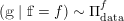 $(\unicode[STIX]{x1D558}\mid \unicode[STIX]{x1D557}=f)\sim \unicode[STIX]{x1D6F1}_{\text{data}}^{f}$
exists (data likelihood) under the joint law
$(\unicode[STIX]{x1D558}\mid \unicode[STIX]{x1D557}=f)\sim \unicode[STIX]{x1D6F1}_{\text{data}}^{f}$
exists (data likelihood) under the joint law
 $\unicode[STIX]{x1D707}$
for any
$\unicode[STIX]{x1D707}$
for any
 $f\in X$
. This allows us to define the data model, which is the statistical analogue of the forward operator, as the following
$f\in X$
. This allows us to define the data model, which is the statistical analogue of the forward operator, as the following
 $\mathscr{P}_{Y}$
-valued mapping defined on
$\mathscr{P}_{Y}$
-valued mapping defined on
 $X$
:
$X$
:
 $$\begin{eqnarray}f\mapsto \unicode[STIX]{x1D6F1}_{\text{data}}^{f}\quad \text{for any }f\in X.\end{eqnarray}$$
Remark 3.3. The existence of regular conditional distributions can be ensured under very general assumptions. In particular, let
 $\unicode[STIX]{x1D557}$
be an
$\unicode[STIX]{x1D557}$
be an
 $X$
-valued random variable and
$X$
-valued random variable and
 $\unicode[STIX]{x1D558}$
a
$\unicode[STIX]{x1D558}$
a
 $Y$
-valued random variable, where
$Y$
-valued random variable, where
 $X$
is a Polish space, i.e. a complete and separable metric space, and
$X$
is a Polish space, i.e. a complete and separable metric space, and
 $Y$
is a general measurable space. Then there exists a regular conditional distribution of the conditional random variable
$Y$
is a general measurable space. Then there exists a regular conditional distribution of the conditional random variable
 $(\unicode[STIX]{x1D557}\mid \unicode[STIX]{x1D558})$
(Kallenberg Reference Kallenberg2002, Theorem 6.3). In particular, when both
$(\unicode[STIX]{x1D557}\mid \unicode[STIX]{x1D558})$
(Kallenberg Reference Kallenberg2002, Theorem 6.3). In particular, when both
 $X$
and
$X$
and
 $X$
are Polish spaces, then both
$X$
are Polish spaces, then both
 $(\unicode[STIX]{x1D557}\mid \unicode[STIX]{x1D558})$
and
$(\unicode[STIX]{x1D557}\mid \unicode[STIX]{x1D558})$
and
 $(\unicode[STIX]{x1D558}\mid \unicode[STIX]{x1D557})$
exist.
$(\unicode[STIX]{x1D558}\mid \unicode[STIX]{x1D557})$
exist.
The most common data model is the statistical analogue of (2.1) where the model parameter is allowed to be a random variable (Kallenberg Reference Kallenberg2002, Lemma 1.28 and Corollary 3.12):
 $$\begin{eqnarray}\unicode[STIX]{x1D558}={\mathcal{A}}(\unicode[STIX]{x1D557})+\unicode[STIX]{x1D556}.\end{eqnarray}$$
Here,
 ${\mathcal{A}}:X\rightarrow Y$
is the same forward operator as in (2.1), which models how data are generated in the absence of noise. Likewise,
${\mathcal{A}}:X\rightarrow Y$
is the same forward operator as in (2.1), which models how data are generated in the absence of noise. Likewise,
 $\unicode[STIX]{x1D556}\sim \unicode[STIX]{x1D6F1}_{\text{noise}}$
, with
$\unicode[STIX]{x1D556}\sim \unicode[STIX]{x1D6F1}_{\text{noise}}$
, with
 $\unicode[STIX]{x1D6F1}_{\text{noise}}\in \mathscr{P}_{Y}$
known, is the random variable that generates the observation noise. If
$\unicode[STIX]{x1D6F1}_{\text{noise}}\in \mathscr{P}_{Y}$
known, is the random variable that generates the observation noise. If
 $\unicode[STIX]{x1D556}$
is independent from
$\unicode[STIX]{x1D556}$
is independent from
 $\unicode[STIX]{x1D557}$
, then (3.2) amounts to the data model
$\unicode[STIX]{x1D557}$
, then (3.2) amounts to the data model
 $$\begin{eqnarray}\unicode[STIX]{x1D6F1}_{\text{data}}^{f}=\unicode[STIX]{x1D6FF}_{{\mathcal{A}}(f)}\circledast \unicode[STIX]{x1D6F1}_{\text{noise}}=\unicode[STIX]{x1D6F1}_{\text{noise}}(\,\cdot \,-{\mathcal{A}}(f))\quad \text{for any }f\in X,\end{eqnarray}$$
where
 $\circledast$
denotes convolution between measures.
$\circledast$
denotes convolution between measures.
Remark 3.4. Another common data model is when
 $\unicode[STIX]{x1D6F1}_{\text{data}}^{f}$
is a Poisson random measure on
$\unicode[STIX]{x1D6F1}_{\text{data}}^{f}$
is a Poisson random measure on
 $Y$
with mean equal to
$Y$
with mean equal to
 ${\mathcal{A}}(f)$
(Hohage and Werner Reference Hohage and Werner2016, Streit Reference Streit2010, Vardi et al.
Reference Vardi, Shepp and Kaufman1985, Besag and Green Reference Besag and Green1993). This is suitable for modelling statistical properties of low-dose imaging data, such as data that is measured in line of response PET (Kadrmas Reference Kadrmas2004, Calvetti and Somersalo Reference Calvetti and Somersalo2008, Section 3.2 of Natterer and Wübbeling Reference Natterer and Wübbeling2001) and variants of fluorescence microscopy (Hell, Schönle and Van den Bos Reference Hell, Schönle, Van den Bos, Hawkes and Spence2007, Diaspro et al.
Reference Diaspro, Schneider, Bianchini, Caorsi, Mazza, Pesce, Testa, Vicidomini, Usai, Hawkes and Spence2007).
${\mathcal{A}}(f)$
(Hohage and Werner Reference Hohage and Werner2016, Streit Reference Streit2010, Vardi et al.
Reference Vardi, Shepp and Kaufman1985, Besag and Green Reference Besag and Green1993). This is suitable for modelling statistical properties of low-dose imaging data, such as data that is measured in line of response PET (Kadrmas Reference Kadrmas2004, Calvetti and Somersalo Reference Calvetti and Somersalo2008, Section 3.2 of Natterer and Wübbeling Reference Natterer and Wübbeling2001) and variants of fluorescence microscopy (Hell, Schönle and Van den Bos Reference Hell, Schönle, Van den Bos, Hawkes and Spence2007, Diaspro et al.
Reference Diaspro, Schneider, Bianchini, Caorsi, Mazza, Pesce, Testa, Vicidomini, Usai, Hawkes and Spence2007).
3.1.2 The inverse problem
Following Evans and Stark (Reference Evans and Stark2002), a (statistical) inverse problem requires us to perform the task of recovering the posterior given a single sample (measured data) from the data model with unknown true model parameter. A more precise statement reads as follows.
Definition 3.5. A statistical inverse problem is the task of recovering the conditional distribution
 $\unicode[STIX]{x1D6F1}_{\text{post}}^{g}\in \mathscr{P}_{Y}$
of
$\unicode[STIX]{x1D6F1}_{\text{post}}^{g}\in \mathscr{P}_{Y}$
of
 $(\unicode[STIX]{x1D557}\mid \unicode[STIX]{x1D558}=g)$
under
$(\unicode[STIX]{x1D557}\mid \unicode[STIX]{x1D558}=g)$
under
 $\unicode[STIX]{x1D707}$
from measured data
$\unicode[STIX]{x1D707}$
from measured data
 $g\in Y$
, where
$g\in Y$
, where
 $$\begin{eqnarray}g\text{ is a single sample of }(\unicode[STIX]{x1D558}\mid \unicode[STIX]{x1D557}=f_{\text{true}})\sim \unicode[STIX]{x1D6F1}_{\text{data}}^{f_{\text{true}}}.\end{eqnarray}$$
Here
 $f_{\text{true}}\in X$
is unknown while
$f_{\text{true}}\in X$
is unknown while
 $f\mapsto \unicode[STIX]{x1D6F1}_{\text{data}}^{f}$
, which describes how data are generated, is known.
$f\mapsto \unicode[STIX]{x1D6F1}_{\text{data}}^{f}$
, which describes how data are generated, is known.
The conceptual difference that comes from adopting such a statistical view brings with it several potential advantages. The posterior, assuming it exists, describes all possible solutions, so recovering it represents a more complete solution to the inverse problem than recovering an approximation of
 $f_{\text{true}}$
, which is the goal in functional analytic regularization. This is particularly the case when one seeks to quantify the uncertainty in the recovered model parameter in terms of statistical properties of the data. However, recovering the entire posterior is often not feasible, such as in inverse problems that arise in imaging. As an alternative, one can settle for exploring the posterior by computing suitable estimators (Section 3.3). Some may serve as approximations of
$f_{\text{true}}$
, which is the goal in functional analytic regularization. This is particularly the case when one seeks to quantify the uncertainty in the recovered model parameter in terms of statistical properties of the data. However, recovering the entire posterior is often not feasible, such as in inverse problems that arise in imaging. As an alternative, one can settle for exploring the posterior by computing suitable estimators (Section 3.3). Some may serve as approximations of
 $f_{\text{true}}$
whereas others are designed for quantifying the uncertainty.
$f_{\text{true}}$
whereas others are designed for quantifying the uncertainty.
3.1.3 Bayes’ theorem
A key part of solving the above inverse problem is to utilize a relation between the unknown posterior that one seeks to recover and the known data likelihood. Such a relation is given by Bayes’ theorem.
A very general formulation of Bayes’ theorem is given by Schervish (Reference Schervish1995, Theorem 1.31). For simplicity we consider the formulation that holds for the special case where the data likelihood is given as in (3.2), with
 ${\mathcal{A}}:X\rightarrow Y$
a measurable map. Assume furthermore that
${\mathcal{A}}:X\rightarrow Y$
a measurable map. Assume furthermore that
 $\unicode[STIX]{x1D557}\sim \unicode[STIX]{x1D6F1}_{\text{prior}}$
and
$\unicode[STIX]{x1D557}\sim \unicode[STIX]{x1D6F1}_{\text{prior}}$
and
 $\unicode[STIX]{x1D556}\sim \unicode[STIX]{x1D6F1}_{\text{noise}}$
, with
$\unicode[STIX]{x1D556}\sim \unicode[STIX]{x1D6F1}_{\text{noise}}$
, with
 $\unicode[STIX]{x1D556}$
independent of
$\unicode[STIX]{x1D556}$
independent of
 $\unicode[STIX]{x1D557}$
. Then the data model is given as in (3.3), that is, at
$\unicode[STIX]{x1D557}$
. Then the data model is given as in (3.3), that is, at
 $f$
it yields the translate of
$f$
it yields the translate of
 $\unicode[STIX]{x1D6F1}_{\text{noise}}$
by
$\unicode[STIX]{x1D6F1}_{\text{noise}}$
by
 ${\mathcal{A}}(f)$
.
${\mathcal{A}}(f)$
.
Assume next that
 $\unicode[STIX]{x1D6F1}_{\text{data}}^{f}\ll \unicode[STIX]{x1D6F1}_{\text{noise}}$
(i.e.
$\unicode[STIX]{x1D6F1}_{\text{data}}^{f}\ll \unicode[STIX]{x1D6F1}_{\text{noise}}$
(i.e.
 $\unicode[STIX]{x1D6F1}_{\text{data}}^{f}$
is absolutely continuous with respect to
$\unicode[STIX]{x1D6F1}_{\text{data}}^{f}$
is absolutely continuous with respect to
 $\unicode[STIX]{x1D6F1}_{\text{noise}}$
)
$\unicode[STIX]{x1D6F1}_{\text{noise}}$
)
 $\unicode[STIX]{x1D6F1}_{\text{noise}}$
-almost surely for all
$\unicode[STIX]{x1D6F1}_{\text{noise}}$
-almost surely for all
 $f\in X$
, so there exists some measurable map
$f\in X$
, so there exists some measurable map
 $\unicode[STIX]{x1D6F7}:X\times Y\rightarrow \mathbb{R}$
(potential) such that
$\unicode[STIX]{x1D6F7}:X\times Y\rightarrow \mathbb{R}$
(potential) such that
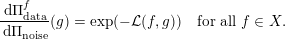 $$\begin{eqnarray}\frac{\,\text{d}\unicode[STIX]{x1D6F1}_{\text{data}}^{f}}{\,\text{d}\unicode[STIX]{x1D6F1}_{\text{noise}}}(g)=\exp (-{\mathcal{L}}(f,g))\quad \text{for all }f\in X.\end{eqnarray}$$
with
 $$\begin{eqnarray}\mathbb{E}_{\unicode[STIX]{x1D558}\sim \unicode[STIX]{x1D6F1}_{\text{noise}}}[\exp (-{\mathcal{L}}(f,\unicode[STIX]{x1D558}))]=1.\end{eqnarray}$$
The mapping
 $f\mapsto -{\mathcal{L}}(f,g)$
is called the (data) log-likelihood for the data
$f\mapsto -{\mathcal{L}}(f,g)$
is called the (data) log-likelihood for the data
 $g\in Y$
.
$g\in Y$
.
Remark 3.6. The equality for the Radon–Nikodym derivative in (3.5) means that
 $$\begin{eqnarray}\mathbb{E}_{\unicode[STIX]{x1D558}\sim \unicode[STIX]{x1D6F1}_{\text{data}}^{f}}[F(\unicode[STIX]{x1D558})]=\mathbb{E}_{\unicode[STIX]{x1D558}\sim \unicode[STIX]{x1D6F1}_{\text{noise}}}[\exp (-{\mathcal{L}}(f,\unicode[STIX]{x1D558}))F(\unicode[STIX]{x1D558})]\end{eqnarray}$$
holds for any measurable
 $F:Y\rightarrow \mathbb{R}$
.
$F:Y\rightarrow \mathbb{R}$
.
Finally, assume
 ${\mathcal{L}}$
is
${\mathcal{L}}$
is
 $\unicode[STIX]{x1D707}_{0}$
-measurable, where
$\unicode[STIX]{x1D707}_{0}$
-measurable, where
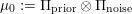 $\unicode[STIX]{x1D707}_{0}:=\unicode[STIX]{x1D6F1}_{\text{prior}}\otimes \unicode[STIX]{x1D6F1}_{\text{noise}}$
and
$\unicode[STIX]{x1D707}_{0}:=\unicode[STIX]{x1D6F1}_{\text{prior}}\otimes \unicode[STIX]{x1D6F1}_{\text{noise}}$
and
 $\unicode[STIX]{x1D707}\ll \unicode[STIX]{x1D707}_{0}$
, which means in particular that the joint law
$\unicode[STIX]{x1D707}\ll \unicode[STIX]{x1D707}_{0}$
, which means in particular that the joint law
 $(\unicode[STIX]{x1D557},\unicode[STIX]{x1D558})\sim \unicode[STIX]{x1D707}$
can be written as
$(\unicode[STIX]{x1D557},\unicode[STIX]{x1D558})\sim \unicode[STIX]{x1D707}$
can be written as
 $$\begin{eqnarray}\frac{\,\text{d}\unicode[STIX]{x1D707}}{\,\text{d}\unicode[STIX]{x1D707}_{0}}(f,g)=\exp (-{\mathcal{L}}(f,g))\quad \text{for }(f,g)\in X\times Y.\end{eqnarray}$$
Bearing in mind the above assumptions, we can now state Bayes’ theorem (Dashti and Stuart Reference Dashti, Stuart and Ghanem2017, Theorem 14), which expresses the posterior in terms of the data likelihood and the prior.
Theorem 3.7 (Bayes’ theorem).
The normalization constant
 $Z:Y\rightarrow \mathbb{R}$
is defined by
$Z:Y\rightarrow \mathbb{R}$
is defined by
 $$\begin{eqnarray}Z(g) :=\mathbb{E}_{\unicode[STIX]{x1D557}\sim \unicode[STIX]{x1D6F1}_{\text{prior}}}[\exp (-{\mathcal{L}}(\unicode[STIX]{x1D557},g))]\end{eqnarray}$$
and we assume
 $Z(g)>0$
holds
$Z(g)>0$
holds
 $\unicode[STIX]{x1D6F1}_{\text{noise}}$
-almost surely for
$\unicode[STIX]{x1D6F1}_{\text{noise}}$
-almost surely for
 $g\in Y$
. Then the posterior
$g\in Y$
. Then the posterior
 $\unicode[STIX]{x1D6F1}_{\text{post}}^{g}$
, which is the conditional distribution of
$\unicode[STIX]{x1D6F1}_{\text{post}}^{g}$
, which is the conditional distribution of
 $(\unicode[STIX]{x1D557}\mid \unicode[STIX]{x1D558}=g)$
, exists under
$(\unicode[STIX]{x1D557}\mid \unicode[STIX]{x1D558}=g)$
, exists under
 $\unicode[STIX]{x1D707}$
and it is absolutely continuous with respect to the prior, i.e.
$\unicode[STIX]{x1D707}$
and it is absolutely continuous with respect to the prior, i.e.
 $\unicode[STIX]{x1D6F1}_{\text{post}}^{g}\ll \unicode[STIX]{x1D6F1}_{\text{prior}}$
. Furthermore,
$\unicode[STIX]{x1D6F1}_{\text{post}}^{g}\ll \unicode[STIX]{x1D6F1}_{\text{prior}}$
. Furthermore,
 $$\begin{eqnarray}\frac{\,\text{d}\unicode[STIX]{x1D6F1}_{\text{post}}^{g}}{\,\text{d}\unicode[STIX]{x1D6F1}_{\text{prior}}}(f)=\frac{1}{Z(g)}\exp (-{\mathcal{L}}(f,g))\end{eqnarray}$$
holds
 $\unicode[STIX]{x1D707}_{0}$
-almost surely for
$\unicode[STIX]{x1D707}_{0}$
-almost surely for
 $(f,g)\in X\times Y$
.
$(f,g)\in X\times Y$
.
Bayes’ theorem is the basis for Bayesian inversion, where one seeks to solve the statistical inverse problem assuming access to both a prior and a data likelihood, whereas
 $f_{\text{true}}\in X$
remains unknown. The data likelihood is given by the data model, which is in turn derived from knowledge about how data are generated. The choice of prior, however, is more subtle: it needs to act as a regularizer, and ideally it also encodes subjective prior beliefs about the unknown model parameter
$f_{\text{true}}\in X$
remains unknown. The data likelihood is given by the data model, which is in turn derived from knowledge about how data are generated. The choice of prior, however, is more subtle: it needs to act as a regularizer, and ideally it also encodes subjective prior beliefs about the unknown model parameter
 $f_{\text{true}}$
by giving high probability to model parameters similar to
$f_{\text{true}}$
by giving high probability to model parameters similar to
 $f_{\text{true}}$
and low probability to other ‘unnatural’ model parameters. A brief survey of hand-crafted priors is provided in Section 3.4.
$f_{\text{true}}$
and low probability to other ‘unnatural’ model parameters. A brief survey of hand-crafted priors is provided in Section 3.4.
3.2 Regularization theory for Bayesian inversion
In functional analytic regularization, existence, stability and convergence are necessary if a reconstruction method is to be a regularization (see Section 2.4). Moreover, a mathematical analysis also seeks to provide convergence rates and stability estimates. There is an ongoing effort to develop a similar theory for Bayesian inversion.
Methods for functional analytic regularization of ill-posed inverse problems typically regularize by a variational procedure or a spectral cut-off. In Bayesian inversion, regularization is mainly through the choice of an appropriate prior distribution. Since many different priors can serve as regularizers, a large portion of the theory seeks to characterize properties of Bayesian inversion methods that are independent of the prior. Much of the analysis in Sections 3.2.3–3.2.5 is therefore performed in the large-sample or small-noise limit, and under the assumption that data
 $g$
is generated from
$g$
is generated from
 $(\unicode[STIX]{x1D558}\mid \unicode[STIX]{x1D557}=f)$
where
$(\unicode[STIX]{x1D558}\mid \unicode[STIX]{x1D557}=f)$
where
 $f=f_{\text{true}}$
(the true model parameter), instead of having
$f=f_{\text{true}}$
(the true model parameter), instead of having
 $f$
as a random sample of
$f$
as a random sample of
 $\unicode[STIX]{x1D557}\sim \unicode[STIX]{x1D6F1}_{\text{prior}}$
(prior).
$\unicode[STIX]{x1D557}\sim \unicode[STIX]{x1D6F1}_{\text{prior}}$
(prior).
Remark 3.8. The parametric setting refers to the case when the dimensions of
 $X$
and
$X$
and
 $Y$
are finite. In this context, a large-sample limit refers to an asymptotic analysis performed when the dimension of
$Y$
are finite. In this context, a large-sample limit refers to an asymptotic analysis performed when the dimension of
 $X$
is kept fixed and independent of the dimension of
$X$
is kept fixed and independent of the dimension of
 $Y$
(sample size), which is allowed to grow. In the non-parametric setting, either both
$Y$
(sample size), which is allowed to grow. In the non-parametric setting, either both
 $Y$
and
$Y$
and
 $X$
are infinite-dimensional from the outset, or one lets the dimension of
$X$
are infinite-dimensional from the outset, or one lets the dimension of
 $X$
increase as the dimension of
$X$
increase as the dimension of
 $Y$
(sample size) increases.
$Y$
(sample size) increases.
3.2.1 Existence
Existence for Bayesian inversion follows when Bayes’ theorem holds. Below we state the precise existence theorem (Dashti and Stuart Reference Dashti, Stuart and Ghanem2017, Theorem 16) for the setting in Section 3.1.3, which covers the case when model parameter and data spaces are infinite-dimensional separable Banach spaces.
Theorem 3.9 (existence for Bayes inversion).
Assume that
 ${\mathcal{L}}:X\times Y\rightarrow \mathbb{R}$
in (3.5) is continuously differentiable on some
${\mathcal{L}}:X\times Y\rightarrow \mathbb{R}$
in (3.5) is continuously differentiable on some
 $X^{\prime }\subset X$
that contains the support of the prior
$X^{\prime }\subset X$
that contains the support of the prior
 $\unicode[STIX]{x1D6F1}_{\text{prior}}$
and
$\unicode[STIX]{x1D6F1}_{\text{prior}}$
and
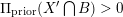 $\unicode[STIX]{x1D6F1}_{\text{prior}}(X^{\prime }\bigcap B)>0$
for some bounded set
$\unicode[STIX]{x1D6F1}_{\text{prior}}(X^{\prime }\bigcap B)>0$
for some bounded set
 $B\subset X$
. Also, assume there exists mappings
$B\subset X$
. Also, assume there exists mappings
 $M_{1},M_{2}:\mathbb{R}_{+}\times \mathbb{R}_{+}\rightarrow \mathbb{R}_{+}$
that are component-wise monotone, non-decreasing and where the following holds:
$M_{1},M_{2}:\mathbb{R}_{+}\times \mathbb{R}_{+}\rightarrow \mathbb{R}_{+}$
that are component-wise monotone, non-decreasing and where the following holds:
 $$\begin{eqnarray}\begin{array}{@{}c@{}}-{\mathcal{L}}(f,g)\leq M_{1}(r,\Vert f\Vert ),\\ |{\mathcal{L}}(f,g)-{\mathcal{L}}(f,v)|\leq M_{2}(r,\Vert f\Vert )\Vert g-v\Vert \end{array}\end{eqnarray}$$
for
 $f\in X$
and
$f\in X$
and
 $g,v\in B_{r}(0)\subset Y$
. Then,
$g,v\in B_{r}(0)\subset Y$
. Then,
 $Z$
in (3.6) is finite, i.e.
$Z$
in (3.6) is finite, i.e.
 $0<Z(g)<\infty$
for any
$0<Z(g)<\infty$
for any
 $g\in Y$
, and the posterior given by (3.7) yields a well-defined
$g\in Y$
, and the posterior given by (3.7) yields a well-defined
 $\mathscr{P}_{X}$
-valued mapping on
$\mathscr{P}_{X}$
-valued mapping on
 $Y$
:
$Y$
:
 $g\mapsto \unicode[STIX]{x1D6F1}_{\text{post}}^{g}$
.
$g\mapsto \unicode[STIX]{x1D6F1}_{\text{post}}^{g}$
.
Under certain circumstances it is possible to work with improper priors on
 $X$
, for example by computing posterior distributions that approximate the posteriors one would have obtained using proper conjugate priors whose extreme values coincide with the improper prior.
$X$
, for example by computing posterior distributions that approximate the posteriors one would have obtained using proper conjugate priors whose extreme values coincide with the improper prior.
3.2.2 Stability
One can show that small changes in the data lead to small changes in the posterior distribution (in Hellinger metric) on
 $\mathscr{P}_{X}$
. The precise formulation given by Dashti and Stuart (Reference Dashti, Stuart and Ghanem2017, Theorem 16) reads as follows.
$\mathscr{P}_{X}$
. The precise formulation given by Dashti and Stuart (Reference Dashti, Stuart and Ghanem2017, Theorem 16) reads as follows.
Theorem 3.10 (stability for Bayes inversion).
Let the assumptions in Theorem 3.9 and assume in addition that
 $$\begin{eqnarray}f\mapsto \exp (M_{1}(r,\Vert f\Vert ))(1+M_{2}(r,\Vert f\Vert ))^{2}\quad \text{is }\unicode[STIX]{x1D6F1}_{\text{prior}}\text{-integrable on }X\end{eqnarray}$$
for some fixed
 $r>0$
. Then
$r>0$
. Then
 $$\begin{eqnarray}d_{\text{H}}(\unicode[STIX]{x1D6F1}_{\text{post}}^{g},\unicode[STIX]{x1D6F1}_{\text{post}}^{v})\leq C(r)\Vert g+v\Vert\end{eqnarray}$$
for some
 $C(r)>0$
and
$C(r)>0$
and
 $g,v\in B_{r}(0)\subset Y$
. In the above,
$g,v\in B_{r}(0)\subset Y$
. In the above,
 $d_{\text{H}}:\mathscr{P}_{X}\times \mathscr{P}_{X}\rightarrow \mathbb{R}$
is the Hellinger metric (see Dashti and Stuart Reference Dashti, Stuart and Ghanem2017, Definition 4).
$d_{\text{H}}:\mathscr{P}_{X}\times \mathscr{P}_{X}\rightarrow \mathbb{R}$
is the Hellinger metric (see Dashti and Stuart Reference Dashti, Stuart and Ghanem2017, Definition 4).
Theorem 3.10 holds in particular when the negative log-likelihood of data is locally Hölder-continuous, which is the case for many standard probability distribution functions, for example when the negative log-likelihood is continuously differentiable.
By Theorem 3.10 the posterior is Lipschitz in the data with respect to the Hellinger metric, so rephrasing the inverse problem as the task of recovering the posterior instead of a model parameter acts as a regularization of an inverse problem that is ill-posed in the functional analytic sense. Note, however, that the above does not automatically imply that a particular estimator is continuous with respect to data. However, the Hellinger distance possesses the convenient property that continuity with respect to this metric implies the continuity of moments. Hence, a corollary to Theorem 3.10 is that posterior moments, such as the mean and covariance, are continuous (Sprungk Reference Sprungk2017, Corollary 3.23), that is, these estimators are regularizing.
As a final note, one can also show that small changes in the data log-likelihood
 ${\mathcal{L}}$
in (3.5) lead to small changes in the posterior distribution, again in the Hellinger metric (Dashti and Stuart Reference Dashti, Stuart and Ghanem2017, Theorem 18). This enables one to translate errors arising from inaccurate forward operator into errors in the Bayesian solution of the inverse problem, a topic that is also considered in Section 6.2.
${\mathcal{L}}$
in (3.5) lead to small changes in the posterior distribution, again in the Hellinger metric (Dashti and Stuart Reference Dashti, Stuart and Ghanem2017, Theorem 18). This enables one to translate errors arising from inaccurate forward operator into errors in the Bayesian solution of the inverse problem, a topic that is also considered in Section 6.2.
3.2.3 Convergence
Posterior consistency is the Bayesian analogue of the notion of convergence in functional analytic regularization. More precisely, the requirement is that the posterior
 $\unicode[STIX]{x1D6F1}_{\text{post}}^{g}$
, where
$\unicode[STIX]{x1D6F1}_{\text{post}}^{g}$
, where
 $g$
is a sample of
$g$
is a sample of
 $(\unicode[STIX]{x1D558}\mid \unicode[STIX]{x1D557}=f_{\text{true}})$
, concentrates in any small neighbourhood of the true model parameter
$(\unicode[STIX]{x1D558}\mid \unicode[STIX]{x1D557}=f_{\text{true}})$
, concentrates in any small neighbourhood of the true model parameter
 $f_{\text{true}}\in X$
as information in data
$f_{\text{true}}\in X$
as information in data
 $g$
increases indefinitely.Footnote
1
Intuitively, this means our knowledge about the model parameter becomes more accurate and precise as the amount of data increases indefinitely.
$g$
increases indefinitely.Footnote
1
Intuitively, this means our knowledge about the model parameter becomes more accurate and precise as the amount of data increases indefinitely.
In the finite-dimensional setting, consistency of the posterior holds if and only if
 $f_{\text{true}}\in X$
is contained in the support of the prior
$f_{\text{true}}\in X$
is contained in the support of the prior
 $\unicode[STIX]{x1D6F1}_{\text{prior}}$
(Freedman Reference Freedman1963, Schwartz Reference Schwartz1965) (provided the posterior is smooth with respect to the model parameter).
$\unicode[STIX]{x1D6F1}_{\text{prior}}$
(Freedman Reference Freedman1963, Schwartz Reference Schwartz1965) (provided the posterior is smooth with respect to the model parameter).
The situation is vastly more complex in the infinite-dimensional (non-parametric) setting. It is known that the posterior is consistent at every model parameter except possibly on a set of measure zero (Doob Reference Doob1948, Breiman, Le Cam and Schwartz Reference Breiman, Le Cam and Schwartz1965), that is, Bayesian inversion is almost always consistent in the measure-theoretic sense. However, the situation changes if ‘smallness’ is measured in a topological sense, as shown by a classical counter-example in Freedman (Reference Freedman1963) involving the simplest non-parametric problem where consistency fails. This is not a pathological counter-example: it is a generic property in the sense that most priors are ‘bad’ in a topological sense (Freedman Reference Freedman1965). In fact, consistency may fail for non-parametric models for very natural priors satisfying the support condition, which means even an infinite amount of data may not be sufficient to ‘correct’ for errors introduced by a prior. Hence, unlike the finite-dimensional setting, many priors do not ‘wash out’ as the information in the data increases indefinitely, so the prior may have a large influence on the corresponding posterior even in the asymptotic setting. Examples of posterior consistency results for Bayesian inversion are given in Ghosal, Ghosh and Ramamoorthi (Reference Ghosal, Ghosh and Ramamoorthi1999), Ghosal, Ghosh and van der Vaart (Reference Ghosal, Ghosh and van der Vaart2000), Neubauer and Pikkarainen (Reference Neubauer and Pikkarainen2008), Bochkina (Reference Bochkina2013), Agapiou, Larsson and Stuart (Reference Agapiou, Larsson and Stuart2013), Stuart and Teckentrup (Reference Stuart and Teckentrup2018), Kekkonen, Lassas and Siltanen (Reference Kekkonen, Lassas and Siltanen2016) and Kleijn and Zhao (Reference Kleijn and Zhao2018).
To summarize, there are many reasonable priors for which posterior consistency holds at every point of the model parameter space
 $X$
. A general class of such ‘good’ priors is that of tail-free priors (Freedman Reference Freedman1963) and neutral-to-the-right priors (Doksum Reference Doksum1974); see also Le Cam (Reference Le Cam1986, Section 17.7). The fact that there are too many ‘bad’ priors may therefore not be such a serious concern since there are also enough good priors approximating any given subjective belief. It is therefore important to have general results providing sufficient conditions for the consistency given a pair of model parameter and prior as developed, and Schwartz (Reference Schwartz1965) is an example in this direction.
$X$
. A general class of such ‘good’ priors is that of tail-free priors (Freedman Reference Freedman1963) and neutral-to-the-right priors (Doksum Reference Doksum1974); see also Le Cam (Reference Le Cam1986, Section 17.7). The fact that there are too many ‘bad’ priors may therefore not be such a serious concern since there are also enough good priors approximating any given subjective belief. It is therefore important to have general results providing sufficient conditions for the consistency given a pair of model parameter and prior as developed, and Schwartz (Reference Schwartz1965) is an example in this direction.
3.2.4 Convergence rates
Posterior consistency is a weak property shared by many different choices of priors. More insight into the performance of Bayesian inversion under the choice of different priors requires characterizing other properties of the posterior, such as quantifying how quickly it converges to the true solution as the observational noise goes to 0. This leads to results about contraction rates, which is the Bayesian analogue of convergence rate theorems in functional analytic regularization.
Formally, consider the setting in (3.2) where the observational noise tends to zero as some scalar
 $\unicode[STIX]{x1D6FF}\rightarrow 0$
, that is, for some fixed
$\unicode[STIX]{x1D6FF}\rightarrow 0$
, that is, for some fixed
 $f_{\text{true}}\in X$
we have
$f_{\text{true}}\in X$
we have
 $$\begin{eqnarray}\unicode[STIX]{x1D558}={\mathcal{A}}(f_{\text{true}})+\unicode[STIX]{x1D556}_{\unicode[STIX]{x1D6FF}}\quad \text{where }\Vert \unicode[STIX]{x1D556}_{\unicode[STIX]{x1D6FF}}\Vert \rightarrow 0\text{ as }\unicode[STIX]{x1D6FF}\rightarrow 0.\end{eqnarray}$$
A contraction rate theorem seeks to find the base rate for
 $\unicode[STIX]{x1D716}(\unicode[STIX]{x1D6FF})\rightarrow 0$
such that
$\unicode[STIX]{x1D716}(\unicode[STIX]{x1D6FF})\rightarrow 0$
such that
 $$\begin{eqnarray}\unicode[STIX]{x1D6F1}_{\text{post}}^{g^{\unicode[STIX]{x1D6FF}}}(\{f\in X:\ell _{X}(f,f_{\text{true}})\geq \unicode[STIX]{x1D716}(\unicode[STIX]{x1D6FF})\})\rightarrow 0\end{eqnarray}$$
 $\unicode[STIX]{x1D6F1}_{\text{post}}^{g_{0}}$
-almost surely as
$\unicode[STIX]{x1D6F1}_{\text{post}}^{g_{0}}$
-almost surely as
 $\unicode[STIX]{x1D716}\rightarrow 0$
. Here,
$\unicode[STIX]{x1D716}\rightarrow 0$
. Here,
 $g^{\unicode[STIX]{x1D6FF}}\in Y$
is a single sample of
$g^{\unicode[STIX]{x1D6FF}}\in Y$
is a single sample of
 $\unicode[STIX]{x1D558}$
in (3.10),
$\unicode[STIX]{x1D558}$
in (3.10),
 $g_{0}={\mathcal{A}}(f_{\text{true}})$
is the corresponding ideal data,
$g_{0}={\mathcal{A}}(f_{\text{true}})$
is the corresponding ideal data,
 $\{\unicode[STIX]{x1D6F1}_{\text{prior}}^{\unicode[STIX]{x1D6FF}}\}_{\unicode[STIX]{x1D6FF}}\subset \mathscr{P}_{X}$
is a sequence of prior distributions with
$\{\unicode[STIX]{x1D6F1}_{\text{prior}}^{\unicode[STIX]{x1D6FF}}\}_{\unicode[STIX]{x1D6FF}}\subset \mathscr{P}_{X}$
is a sequence of prior distributions with
 $f\sim \unicode[STIX]{x1D6F1}_{\text{prior}}^{\unicode[STIX]{x1D6FF}}$
, and
$f\sim \unicode[STIX]{x1D6F1}_{\text{prior}}^{\unicode[STIX]{x1D6FF}}$
, and
 $\ell _{X}:X\times X\rightarrow \mathbb{R}$
is a (measurable) distance function on
$\ell _{X}:X\times X\rightarrow \mathbb{R}$
is a (measurable) distance function on
 $X$
. Research in this area has mainly focused on (a) obtaining contraction rates for Bayesian inversion where the prior is from some large class, or (b) improving the rates by changing the parameters of the prior depending on the level of noise (and even the data). Most of the work is done for additive observational white Gaussian noise, that is, the setting in (3.10) with
$X$
. Research in this area has mainly focused on (a) obtaining contraction rates for Bayesian inversion where the prior is from some large class, or (b) improving the rates by changing the parameters of the prior depending on the level of noise (and even the data). Most of the work is done for additive observational white Gaussian noise, that is, the setting in (3.10) with
 $\unicode[STIX]{x1D556}_{\unicode[STIX]{x1D6FF}}=\unicode[STIX]{x1D6FF}W$
, where
$\unicode[STIX]{x1D556}_{\unicode[STIX]{x1D6FF}}=\unicode[STIX]{x1D6FF}W$
, where
 $W$
is a centred Gaussian white noise process that can be defined by its action on a separable Hilbert space
$W$
is a centred Gaussian white noise process that can be defined by its action on a separable Hilbert space
 $Y$
. See Dashti and Stuart (Reference Dashti, Stuart and Ghanem2017, Sections A.3 and A.4) for a survey related to Gaussian measures and Wiener processes on separable Banach spaces.
$Y$
. See Dashti and Stuart (Reference Dashti, Stuart and Ghanem2017, Sections A.3 and A.4) for a survey related to Gaussian measures and Wiener processes on separable Banach spaces.
As one might expect, initial results were for linear forward operators. The first results restricted attention to conjugate priors where the posterior has an explicit expression (it is in the same family as the prior) (Liese and Miescke Reference Liese and Miescke2008, Section 1.2). However, Bayesian non-parametric statistics often carries over to the inverse setting via the singular value decomposition of the linear forward operator. This allowed one to prove contraction rate results for Bayesian inversion with non-conjugate priors (Knapik, van der Vaart and van Zanten Reference Knapik, van der Vaart and van Zanten2011, Knapik, van der Vaart and van Zanten Reference Knapik, van der Vaart and van Zanten2013, Ray Reference Ray2013, Agapiou et al. Reference Agapiou, Larsson and Stuart2013, Agapiou, Stuart and Zhang Reference Agapiou, Stuart and Zhang2014). In particular, if the Gaussian prior is non-diagonal for the singular value decomposition (SVD), then the posterior is still Gaussian and its contraction rate will be driven by the convergence rate of its posterior mean (since the variance does not depend on the data). Furthermore, in the linear setting, the posterior mean is the MAP, so the convergence rate of the MAP will be a posterior contraction rate.
Unfortunately, not many of the methods developed for proving contraction rates in the linear setting carry over to proving contraction rates for general, non-linear, inverse problems. A specific difficulty in the Bayesian setting is that the noise term often does not take values in the natural range of the forward operator. For example, consider the data model in (3.3) with observational white Gaussian noise, i.e. (3.10) with
 $\unicode[STIX]{x1D556}_{\unicode[STIX]{x1D6FF}}=\unicode[STIX]{x1D6FF}W$
, where
$\unicode[STIX]{x1D556}_{\unicode[STIX]{x1D6FF}}=\unicode[STIX]{x1D6FF}W$
, where
 $W$
is a centred Gaussian white noise process that can be defined by its action on a separable Hilbert space
$W$
is a centred Gaussian white noise process that can be defined by its action on a separable Hilbert space
 $Y$
. If we have a non-linear forward operator
$Y$
. If we have a non-linear forward operator
 ${\mathcal{A}}$
given as the solution operator to an elliptic PDE, then the noise process
${\mathcal{A}}$
given as the solution operator to an elliptic PDE, then the noise process
 $W$
does not define a proper random element in
$W$
does not define a proper random element in
 $Y=L^{2}(\mathbb{M})$
for
$Y=L^{2}(\mathbb{M})$
for
 $\mathbb{M}\subset \mathbb{R}^{d}$
: instead it defines a random variable only in a negative Sobolev space
$\mathbb{M}\subset \mathbb{R}^{d}$
: instead it defines a random variable only in a negative Sobolev space
 $W^{-\unicode[STIX]{x1D6FD}}$
with
$W^{-\unicode[STIX]{x1D6FD}}$
with
 $\unicode[STIX]{x1D6FD}>d/2$
. Nevertheless, there are also some results in the non-linear setting: for example, Kekkonen et al. (Reference Kekkonen, Lassas and Siltanen2016) derive contraction rate results for Bayesian inversion of inverse problems under Gaussian conjugate priors and where the forward operator is a linear hypoelliptic pseudodifferential operator. Recent developments that make use of techniques from concentration of measure theory have resulted in contraction rate theorems outside the conjugate setting. For example, Nickl and Söhl (Reference Nickl and Söhl2017) and Nickl (Reference Nickl2017a
) derive contraction rates for Bayesian inversion for parameter estimation involving certain classes of elliptic PDEs that are minimax-optimal in prediction loss: see e.g. Nickl (Reference Nickl2017a
, Theorem 28) for an example of a general contraction theorem. The case of a (possibly) non-linear forward operator and a Gaussian prior is considered in Nickl, van de Geer and Wang (Reference Nickl, van de Geer and Wang2018), which studies properties of the MAP estimator. Finally, Gugushvili, van der Vaart and Yan (Reference Gugushvili, van der Vaart and Yan2018) derive contraction rates for ‘general’ priors expressed by scales of smoothness classes. The precise conditions are checked only for an elliptic example: it is not clear whether it works in other examples, such as the ray transform.
$\unicode[STIX]{x1D6FD}>d/2$
. Nevertheless, there are also some results in the non-linear setting: for example, Kekkonen et al. (Reference Kekkonen, Lassas and Siltanen2016) derive contraction rate results for Bayesian inversion of inverse problems under Gaussian conjugate priors and where the forward operator is a linear hypoelliptic pseudodifferential operator. Recent developments that make use of techniques from concentration of measure theory have resulted in contraction rate theorems outside the conjugate setting. For example, Nickl and Söhl (Reference Nickl and Söhl2017) and Nickl (Reference Nickl2017a
) derive contraction rates for Bayesian inversion for parameter estimation involving certain classes of elliptic PDEs that are minimax-optimal in prediction loss: see e.g. Nickl (Reference Nickl2017a
, Theorem 28) for an example of a general contraction theorem. The case of a (possibly) non-linear forward operator and a Gaussian prior is considered in Nickl, van de Geer and Wang (Reference Nickl, van de Geer and Wang2018), which studies properties of the MAP estimator. Finally, Gugushvili, van der Vaart and Yan (Reference Gugushvili, van der Vaart and Yan2018) derive contraction rates for ‘general’ priors expressed by scales of smoothness classes. The precise conditions are checked only for an elliptic example: it is not clear whether it works in other examples, such as the ray transform.
Remark 3.11. The proof techniques used for obtaining contraction rates in the non-linear setting depend on stability estimates for the forward problem that allow us to control
 $\Vert f-h\Vert$
in terms of
$\Vert f-h\Vert$
in terms of
 $\Vert {\mathcal{A}}(f)-{\mathcal{A}}(h)\Vert$
in some suitable norm, and a dual form of the usual regularity estimates for solutions of PDEs that encodes the (functional analytic) ill-posedness of the problem. With estimates, one can use methods from non-parametric statistics to prove contraction rates for Bayesian inversion, with priors that do not require identifying a singular value-type basis underlying the forward operator.
$\Vert {\mathcal{A}}(f)-{\mathcal{A}}(h)\Vert$
in some suitable norm, and a dual form of the usual regularity estimates for solutions of PDEs that encodes the (functional analytic) ill-posedness of the problem. With estimates, one can use methods from non-parametric statistics to prove contraction rates for Bayesian inversion, with priors that do not require identifying a singular value-type basis underlying the forward operator.
3.2.5 Characterization of the posterior for uncertainty quantification
Posterior consistency and contraction rates are relevant results, but assessing the performance of Bayesian inversion methods in uncertainty quantification requires a more precise characterization of the posterior. The aim is to characterize the fluctuations of
 $(\unicode[STIX]{x1D557}\mid \unicode[STIX]{x1D558}=g)$
near
$(\unicode[STIX]{x1D557}\mid \unicode[STIX]{x1D558}=g)$
near
 $f_{\text{true}}$
when scaled by some inverse contraction rate.
$f_{\text{true}}$
when scaled by some inverse contraction rate.
One approach is to derive Bernstein–von Mises type theorems, which characterize the posterior distribution in terms of a canonical Gaussian distribution in the small-noise or large-sample limit. To better illustrate the role of such theorems, we consider the special case with Gaussian prior on the Hilbert space
 $X$
and observational noise
$X$
and observational noise
 $\unicode[STIX]{x1D556}_{\unicode[STIX]{x1D6FF}}=\unicode[STIX]{x1D6FF}\mathbb{W}$
in (3.10) (white noise model) where
$\unicode[STIX]{x1D556}_{\unicode[STIX]{x1D6FF}}=\unicode[STIX]{x1D6FF}\mathbb{W}$
in (3.10) (white noise model) where
 $\mathbb{W}$
denotes a Gaussian white noise process in the Hilbert space
$\mathbb{W}$
denotes a Gaussian white noise process in the Hilbert space
 $Y$
, that is,
$Y$
, that is,
 $$\begin{eqnarray}\unicode[STIX]{x1D558}^{\unicode[STIX]{x1D6FF}}={\mathcal{A}}(f_{\text{true}})+\unicode[STIX]{x1D6FF}\mathbb{W}.\end{eqnarray}$$
Many of the results on contraction rates (Section 3.2.4) for Bayesian inversion in this setting are obtained for the distance function induced by the
 $L^{2}$
-norm, so it is natural to initially consider the statistical fluctuations in
$L^{2}$
-norm, so it is natural to initially consider the statistical fluctuations in
 $L^{2}$
of the random variable
$L^{2}$
of the random variable
 $$\begin{eqnarray}\unicode[STIX]{x1D56B}_{\unicode[STIX]{x1D6FF}} :=\frac{1}{\unicode[STIX]{x1D716}_{\unicode[STIX]{x1D6FF}}}(\mathbb{E}[\unicode[STIX]{x1D557}\mid \unicode[STIX]{x1D558}=g^{\unicode[STIX]{x1D6FF}}]-f_{\text{true}}).\end{eqnarray}$$
Now, it turns out that there is no Bernstein–von Mises type asymptotics for
 $\unicode[STIX]{x1D56B}_{\unicode[STIX]{x1D6FF}}$
as the noise level
$\unicode[STIX]{x1D56B}_{\unicode[STIX]{x1D6FF}}$
as the noise level
 $\unicode[STIX]{x1D6FF}$
tends to zero, that is, there is no Gaussian process
$\unicode[STIX]{x1D6FF}$
tends to zero, that is, there is no Gaussian process
 $(\mathbb{G}(\unicode[STIX]{x1D719}))_{\unicode[STIX]{x1D719}\in C^{\infty }}$
such that
$(\mathbb{G}(\unicode[STIX]{x1D719}))_{\unicode[STIX]{x1D719}\in C^{\infty }}$
such that
 $$\begin{eqnarray}\biggl(\frac{1}{\unicode[STIX]{x1D6FF}}\langle \unicode[STIX]{x1D56B}_{\unicode[STIX]{x1D6FF}}-\mathbb{E}[\unicode[STIX]{x1D56B}_{\unicode[STIX]{x1D6FF}}],\unicode[STIX]{x1D719}\rangle _{L^{2}}\biggr)_{\unicode[STIX]{x1D719}\in C^{\infty }}\rightarrow (\mathbb{G}(\unicode[STIX]{x1D719}))_{\unicode[STIX]{x1D719}\in C^{\infty }}\quad \text{weakly as }\unicode[STIX]{x1D6FF}\rightarrow 0.\end{eqnarray}$$
To sidestep this difficulty, Castillo and Nickl (Reference Castillo and Nickl2013, Reference Castillo and Nickl2014) seek to determine maximal families
 $\unicode[STIX]{x1D6F9}$
that replace
$\unicode[STIX]{x1D6F9}$
that replace
 $C^{\infty }$
in (3.11) and where such an asymptotic characterization holds. This leads to non-parametric Bernstein–von Mises theorems, and while Castillo and Nickl (Reference Castillo and Nickl2013, Reference Castillo and Nickl2014) considered ‘direct’ problems in non-parametric regression and probability density estimation, recent papers have obtained non-parametric Bernstein–von Mises theorems for certain classes of inverse problems. For example, Monard, Nickl and Paternain (Reference Monard, Nickl and Paternain2019) consider the case of inverting the (generalized) ray transform, whereas Nickl (Reference Nickl2017a
) considers PDE parameter estimation problems. The case with general linear forward problem is treated by Giordano and Kekkonen (Reference Giordano and Kekkonen2018), who build upon the techniques of Monard et al. (Reference Monard, Nickl and Paternain2019).
$C^{\infty }$
in (3.11) and where such an asymptotic characterization holds. This leads to non-parametric Bernstein–von Mises theorems, and while Castillo and Nickl (Reference Castillo and Nickl2013, Reference Castillo and Nickl2014) considered ‘direct’ problems in non-parametric regression and probability density estimation, recent papers have obtained non-parametric Bernstein–von Mises theorems for certain classes of inverse problems. For example, Monard, Nickl and Paternain (Reference Monard, Nickl and Paternain2019) consider the case of inverting the (generalized) ray transform, whereas Nickl (Reference Nickl2017a
) considers PDE parameter estimation problems. The case with general linear forward problem is treated by Giordano and Kekkonen (Reference Giordano and Kekkonen2018), who build upon the techniques of Monard et al. (Reference Monard, Nickl and Paternain2019).
To give a flavour of the type of results obtained, we consider Theorem 2.5 of Monard et al. (Reference Monard, Nickl and Paternain2019), which is relevant to tomographic inverse problems involving inversion of the ray transform for recovering a function (images) defined on
 $\unicode[STIX]{x1D6FA}\subset \mathbb{R}^{d}$
, i.e.
$\unicode[STIX]{x1D6FA}\subset \mathbb{R}^{d}$
, i.e.
 $X\subset L^{2}(\unicode[STIX]{x1D6FA})$
. This theorem states that
$X\subset L^{2}(\unicode[STIX]{x1D6FA})$
. This theorem states that
 $$\begin{eqnarray}\frac{1}{\unicode[STIX]{x1D6FF}}\langle (\unicode[STIX]{x1D557}\mid \unicode[STIX]{x1D558}=g^{\unicode[STIX]{x1D6FF}})-\mathbb{E}[\unicode[STIX]{x1D557}|\unicode[STIX]{x1D558}=g^{\unicode[STIX]{x1D6FF}}],\unicode[STIX]{x1D719}\rangle _{L^{2}}\rightarrow \operatorname{N}(0,\Vert {\mathcal{A}}\circ ({\mathcal{A}}^{\ast }\circ {\mathcal{A}})^{-1}(\unicode[STIX]{x1D719})\Vert _{Y})\end{eqnarray}$$
as
 $\unicode[STIX]{x1D6FF}\rightarrow 0$
for any
$\unicode[STIX]{x1D6FF}\rightarrow 0$
for any
 $\unicode[STIX]{x1D719}\in C^{\infty }(\unicode[STIX]{x1D6FA})$
.
$\unicode[STIX]{x1D719}\in C^{\infty }(\unicode[STIX]{x1D6FA})$
.
The convergence is in
 $\unicode[STIX]{x1D6F1}_{\text{prior}}$
-probability and the
$\unicode[STIX]{x1D6F1}_{\text{prior}}$
-probability and the
 $Y$
-norm on the right-hand side is a natural
$Y$
-norm on the right-hand side is a natural
 $L^{2}$
-norm on the range of the ray transform. The limiting covariance is also shown to be minimal, that is, it attains the semi-parametric Cramér–Rao lower bound (or ‘inverse Fisher information’) for estimating
$L^{2}$
-norm on the range of the ray transform. The limiting covariance is also shown to be minimal, that is, it attains the semi-parametric Cramér–Rao lower bound (or ‘inverse Fisher information’) for estimating
 $\langle f,\unicode[STIX]{x1D719}\rangle _{L^{2}}$
near
$\langle f,\unicode[STIX]{x1D719}\rangle _{L^{2}}$
near
 $f_{\text{true}}$
. A key step in the proof is to show smoothness of the ‘Fisher information’ operator
$f_{\text{true}}$
. A key step in the proof is to show smoothness of the ‘Fisher information’ operator
 $({\mathcal{A}}^{\ast }\circ {\mathcal{A}})^{-1}:X\rightarrow X$
, which is done using techniques from microlocal analysis (Monard et al.
Reference Monard, Nickl and Paternain2019, Theorem 2.2). The existence and mapping properties of this inverse Fisher information operator in (3.12) also plays a crucial role in proving that Bernstein–von Mises theorem for other inverse problems. For those with a non-linear forward operator, the information operator to be inverted is found after linearization as shown in Nickl (Reference Nickl2017a
) for parameter estimation in an elliptic PDE.
$({\mathcal{A}}^{\ast }\circ {\mathcal{A}})^{-1}:X\rightarrow X$
, which is done using techniques from microlocal analysis (Monard et al.
Reference Monard, Nickl and Paternain2019, Theorem 2.2). The existence and mapping properties of this inverse Fisher information operator in (3.12) also plays a crucial role in proving that Bernstein–von Mises theorem for other inverse problems. For those with a non-linear forward operator, the information operator to be inverted is found after linearization as shown in Nickl (Reference Nickl2017a
) for parameter estimation in an elliptic PDE.
Relevance to applications.
For large-scale problems, such as those arising in imaging, it is computationally challenging to even explore the posterior beyond computing point estimators (Section 3.5). This holds in particular for the task of computing Bayesian credible sets, which are relevant for uncertainty quantification. Hence, the theoretical results in Section 3.2.5 can be of interest in practical applications, since these provide good analytic approximations of the posterior that are much simpler to compute.
In particular, if a Bernstein–von Mises theorem holds, then the Bayesian and maximum likelihood estimators have the same asymptotic properties and the influence of the prior diminishes asymptotically as information in the data increases. Then, Bayesian credible sets are asymptotically equivalent to frequentist confidence regions,Footnote 2 so Bayesian inversion with 95% posterior credibility will have approximately 0.95 chance of returning the correct decision in repeated trials.
Many of the results, however, assume a Gaussian prior and data likelihood: for non-Gaussian problems in an infinite-dimensional setting the structure of the posterior can be very chaotic and difficult to characterize. Furthermore, the issue with any such asymptotic characterization of the posterior is that it is based on increasing information in data indefinitely. In reality data are fixed, and it is quite possible that the posterior is (very) non-normal and possibly multi-modal even though it behaves asymptotically like a Gaussian (or more generally the sampling distribution of a maximum likelihood estimator). Hence, a regularizing prior that provides ‘best’ contraction rates may not necessarily be the best when it comes to image quality for data with a given noise level. Here one would need to consider a prior that acts as more than just a regularizer. Finally, the assumptions of the Bernstein–von Mises theorem are fragile and easy to violate for a dataset or analysis, and it is difficult to know, without outside information, when this will occur. As nicely outlined in Nickl (Reference Nickl2013, Section 2.25), the parametric (finite-dimensional) setting already requires many assumptions, such as a consistent maximum likelihood estimator, a true model parameter in the support of the prior, and a log-likelihood that is sufficiently regular. For example, data in an inverse problem are observational, and therefore it is unlikely that an estimator of
 $f_{\text{true}}$
, such as maximum likelihood or the posterior mean, is consistent, in which case a Bernstein–von Mises theorem does not apply.
$f_{\text{true}}$
, such as maximum likelihood or the posterior mean, is consistent, in which case a Bernstein–von Mises theorem does not apply.
3.3 Reconstruction method as a point estimator
In most large-scale inverse problems it is computationally very challenging, if not impossible, to recover the entire posterior. However, a reconstruction method that seeks to compute an estimator for the posterior formally defines a mapping
 ${\mathcal{R}}:Y\rightarrow X$
(reconstruction operator). As such, it can be viewed as non-randomized decision rule (point estimator) in a statistical estimation problem: see Liese and Miescke (Reference Liese and Miescke2008, Definition 3.1) for the formal definition. Computing a suitable point estimator is therefore an alternative to seeking to recover the posterior.
${\mathcal{R}}:Y\rightarrow X$
(reconstruction operator). As such, it can be viewed as non-randomized decision rule (point estimator) in a statistical estimation problem: see Liese and Miescke (Reference Liese and Miescke2008, Definition 3.1) for the formal definition. Computing a suitable point estimator is therefore an alternative to seeking to recover the posterior.
In the infinite-dimensional setting, the benefits of using one estimator rather than another (e.g. the conditional mean estimate rather than the MAP estimate) are not well understood. Statistical decision theory provides criteria for selecting and comparing decision rules, which can be used when selecting the estimator (reconstruction method). This requires phrasing the inverse problem as a statistical decision problem. More precisely, the tuple
 $((Y,\mathfrak{S}_{Y}),\{\unicode[STIX]{x1D6F1}_{\text{data}}^{f}\}_{f\in X})$
defines a statistical model which is parametrized by the Banach space
$((Y,\mathfrak{S}_{Y}),\{\unicode[STIX]{x1D6F1}_{\text{data}}^{f}\}_{f\in X})$
defines a statistical model which is parametrized by the Banach space
 $X$
. The inverse problem is now a statistical decision problem (Liese and Miescke Reference Liese and Miescke2008, Definition 3.4) where the statistical model is parametrized by
$X$
. The inverse problem is now a statistical decision problem (Liese and Miescke Reference Liese and Miescke2008, Definition 3.4) where the statistical model is parametrized by
 $X$
, the decision space is
$X$
, the decision space is
 $D:=X$
, and a given loss function:
$D:=X$
, and a given loss function:
 $$\begin{eqnarray}\ell _{X}:X\times X\rightarrow \mathbb{R}.\end{eqnarray}$$
The loss function is used to define the risk, which is given as the
 $\unicode[STIX]{x1D6F1}_{\text{data}}^{f}$
-expectation of the loss function. The risk seeks to quantify the downside that comes with using a particular reconstruction operator
$\unicode[STIX]{x1D6F1}_{\text{data}}^{f}$
-expectation of the loss function. The risk seeks to quantify the downside that comes with using a particular reconstruction operator
 ${\mathcal{R}}:Y\rightarrow X$
.
${\mathcal{R}}:Y\rightarrow X$
.
3.3.1 Some point estimators
Here we briefly define the most common point estimators that are commonly considered in solving many inverse problems. Overall, estimators that include an integration over
 $X$
are computationally demanding. These include the conditional mean and many estimators associated with uncertainty quantification.
$X$
are computationally demanding. These include the conditional mean and many estimators associated with uncertainty quantification.
Maximum likelihood estimator.
This estimator maximizes the data likelihood. Under the data model in (3.5), the (maximum likelihood) reconstruction operator
 ${\mathcal{R}}:Y\rightarrow X$
becomes
${\mathcal{R}}:Y\rightarrow X$
becomes
The advantage of the maximum likelihood estimator is that it does not involve any integration over
 $X$
, so it is computationally feasible to use on large-scale problems. Furthermore, it only requires access to the data likelihood (no need to specify a prior), which is known. On the other hand, it does not act as a regularizer, so it is not suitable for ill-posed problems.
$X$
, so it is computationally feasible to use on large-scale problems. Furthermore, it only requires access to the data likelihood (no need to specify a prior), which is known. On the other hand, it does not act as a regularizer, so it is not suitable for ill-posed problems.
Maximum a posteriori (MAP) estimator.
This estimator maximizes the posterior probability, that is, it is the ‘most likely’ model parameter given measured data
 $g$
. In the finite-dimensional setting, the prior and posterior distribution can typically be described by densities with respect to the Lebesgue measure, and the MAP estimator is defined as the reconstruction operator
$g$
. In the finite-dimensional setting, the prior and posterior distribution can typically be described by densities with respect to the Lebesgue measure, and the MAP estimator is defined as the reconstruction operator
 ${\mathcal{R}}:Y\rightarrow X$
given by
${\mathcal{R}}:Y\rightarrow X$
given by
The second equality above assumes a data model as in (3.5).
For many of the infinite-dimensional spaces there exists no analogue of the Lebesgue measure, which makes it difficult to define a MAP estimator through densities. One way to work around this technical problem is to replace the Lebesgue measure with a Gaussian measure on
 $X$
. Hence, we assume the posterior and prior have densities with respect to some fixed centred (mean-zero) Gaussian measure
$X$
. Hence, we assume the posterior and prior have densities with respect to some fixed centred (mean-zero) Gaussian measure
 $\unicode[STIX]{x1D707}_{0}$
and
$\unicode[STIX]{x1D707}_{0}$
and
 $E$
denotes its Cameron–Martin space.Footnote
3
Now, following Dashti, Law, Stuart and Voss (Reference Dashti, Law, Stuart and Voss2013), we consider the centre of a small ball in
$E$
denotes its Cameron–Martin space.Footnote
3
Now, following Dashti, Law, Stuart and Voss (Reference Dashti, Law, Stuart and Voss2013), we consider the centre of a small ball in
 $X$
with maximal probability, and then study the limit of this centre as the radius of the ball shrinks to zero. Stated precisely, given fixed data
$X$
with maximal probability, and then study the limit of this centre as the radius of the ball shrinks to zero. Stated precisely, given fixed data
 $g\in Y$
, assume there is a functional
$g\in Y$
, assume there is a functional
 ${\mathcal{J}}:E\rightarrow \mathbb{R}$
that satisfies
${\mathcal{J}}:E\rightarrow \mathbb{R}$
that satisfies
 $$\begin{eqnarray}\lim _{r\rightarrow 0}\frac{\unicode[STIX]{x1D6F1}_{\text{post}}^{g}(B_{r}(f_{1}))}{\unicode[STIX]{x1D6F1}_{\text{post}}^{g}(B_{r}(f_{2}))}=\exp ({\mathcal{J}}(f_{1})-{\mathcal{J}}(f_{2})).\end{eqnarray}$$
Here,
 $B_{r}(f)\subset X$
is the open ball of radius
$B_{r}(f)\subset X$
is the open ball of radius
 $r>0$
centred at
$r>0$
centred at
 $f\in X$
and
$f\in X$
and
 ${\mathcal{J}}$
is the Onsager–Machlup functional (Ikeda and Watanabe Reference Ikeda and Watanabe1989, p. 533).
${\mathcal{J}}$
is the Onsager–Machlup functional (Ikeda and Watanabe Reference Ikeda and Watanabe1989, p. 533).
For any fixed
 $f_{1}\in X$
, a model parameter
$f_{1}\in X$
, a model parameter
 $f_{2}\in X$
for which the above limit is maximal is a natural candidate for the MAP estimator and is clearly given by minimizers of the Onsager–Machlup functional. The advantage of the MAP estimator is that it does not involve any integration over
$f_{2}\in X$
for which the above limit is maximal is a natural candidate for the MAP estimator and is clearly given by minimizers of the Onsager–Machlup functional. The advantage of the MAP estimator is that it does not involve any integration over
 $X$
. Furthermore, the prior often acts as a regularizer, so MAP can be useful for solving an ill-posed inverse problem. A disadvantage is that a MAP may not always exist (Section 3.3.2): one needs to provide an explicit prior, and many priors result in a non-smooth optimization problem. Due to the latter, MAP estimation is computationally more challenging than maximum likelihood estimation.
$X$
. Furthermore, the prior often acts as a regularizer, so MAP can be useful for solving an ill-posed inverse problem. A disadvantage is that a MAP may not always exist (Section 3.3.2): one needs to provide an explicit prior, and many priors result in a non-smooth optimization problem. Due to the latter, MAP estimation is computationally more challenging than maximum likelihood estimation.
Conditional (posterior) mean.
The reconstruction operator
 ${\mathcal{R}}:Y\rightarrow X$
is here defined as
${\mathcal{R}}:Y\rightarrow X$
is here defined as
 $$\begin{eqnarray}{\mathcal{R}}(g):=\mathbb{E}[\unicode[STIX]{x1D557}\mid \unicode[STIX]{x1D558}=g]=\int _{X}f\,\,\text{d}\unicode[STIX]{x1D6F1}_{\text{post}}^{g}(f).\end{eqnarray}$$
This estimator involves integration over
 $X$
, making it challenging to use on even small- to mid-scale problems. It also assumes access to the posterior, which in turn requires a prior. It does, however, act as a regularizer (Sprungk Reference Sprungk2017, Corollary 3.23) and therefore it is suitable for ill-posed problems.
$X$
, making it challenging to use on even small- to mid-scale problems. It also assumes access to the posterior, which in turn requires a prior. It does, however, act as a regularizer (Sprungk Reference Sprungk2017, Corollary 3.23) and therefore it is suitable for ill-posed problems.
Bayes estimator.
One starts by specifying a function
 $\ell _{X}:X\times X\rightarrow \mathbb{R}$
that quantifies proximity in
$\ell _{X}:X\times X\rightarrow \mathbb{R}$
that quantifies proximity in
 $X$
(it does not have to be a metric). Then, a Bayes estimator minimizes the expected loss with respect to the prior
$X$
(it does not have to be a metric). Then, a Bayes estimator minimizes the expected loss with respect to the prior
 $\unicode[STIX]{x1D6F1}_{\text{prior}}$
, that is,
$\unicode[STIX]{x1D6F1}_{\text{prior}}$
, that is,
 ${\mathcal{R}}:Y\rightarrow X$
is defined as
${\mathcal{R}}:Y\rightarrow X$
is defined as
This estimator is challenging to compute even for small- to mid-scale problems, due to the integration over
 $X\times Y$
and the minimization over all non-randomized decision rules. It also requires access to the joint distribution
$X\times Y$
and the minimization over all non-randomized decision rules. It also requires access to the joint distribution
 $\unicode[STIX]{x1D707}$
, which by the law of total probability is expressible as
$\unicode[STIX]{x1D707}$
, which by the law of total probability is expressible as
 $\unicode[STIX]{x1D707}=\unicode[STIX]{x1D6F1}_{\text{prior}}\otimes \unicode[STIX]{x1D6F1}_{\text{data}}^{f}$
with known data likelihood
$\unicode[STIX]{x1D707}=\unicode[STIX]{x1D6F1}_{\text{prior}}\otimes \unicode[STIX]{x1D6F1}_{\text{data}}^{f}$
with known data likelihood
 $\unicode[STIX]{x1D6F1}_{\text{data}}^{f}$
. An important property of the Bayes estimator is that it is a regularizer, so it is suitable for ill-posed problems. It is also equivalent to the conditional mean when the loss is taken as the square of the
$\unicode[STIX]{x1D6F1}_{\text{data}}^{f}$
. An important property of the Bayes estimator is that it is a regularizer, so it is suitable for ill-posed problems. It is also equivalent to the conditional mean when the loss is taken as the square of the
 $L^{2}$
-norm (Helin and Burger Reference Helin and Burger2015) and the conditional median when the loss is the
$L^{2}$
-norm (Helin and Burger Reference Helin and Burger2015) and the conditional median when the loss is the
 $L^{1}$
-norm. Furthermore, Theorem 1 of Burger and Lucka (Reference Burger and Lucka2014) shows that a MAP estimator with a Gibbs-type prior where the energy functional is Lipschitz-continuous and convex equals a Bayes estimator where the loss is the Bregman distance of the aforementioned energy functional. Finally, in the finite-dimensional setting, one can show (Banerjee, Guo and Wang Reference Banerjee, Guo and Wang2005) that the Bayes estimator is the same as the conditional mean if and only if
$L^{1}$
-norm. Furthermore, Theorem 1 of Burger and Lucka (Reference Burger and Lucka2014) shows that a MAP estimator with a Gibbs-type prior where the energy functional is Lipschitz-continuous and convex equals a Bayes estimator where the loss is the Bregman distance of the aforementioned energy functional. Finally, in the finite-dimensional setting, one can show (Banerjee, Guo and Wang Reference Banerjee, Guo and Wang2005) that the Bayes estimator is the same as the conditional mean if and only if
 $\ell _{X}$
is the Bregman distance of a strictly convex non-negative differentiable functional.Footnote
4
$\ell _{X}$
is the Bregman distance of a strictly convex non-negative differentiable functional.Footnote
4
Other estimators.
Another important family of estimators in statistical decision theory is that of minimax estimators that minimize the maximum loss. Estimators for uncertainty quantification typically involve higher-order moments, such as the variance, or interval estimators that are given as a set of points in the model parameter space
 $X$
.
$X$
.
3.3.2 Relation to functional analytic regularization
It is quite common to interpret a variational method as in (2.7) as a MAP estimators. This is especially the case when one chooses the data discrepancy
 ${\mathcal{L}}$
so that minimizing
${\mathcal{L}}$
so that minimizing
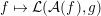 $f\mapsto {\mathcal{L}}({\mathcal{A}}(f),g)$
corresponds to computing a maximum likelihood estimator.
$f\mapsto {\mathcal{L}}({\mathcal{A}}(f),g)$
corresponds to computing a maximum likelihood estimator.
Such an interpretation is almost always possible in the finite-dimensional setting since, as mentioned in Definition 2.2, the regularization functional
 ${\mathcal{S}}_{\unicode[STIX]{x1D703}}$
can be interpreted as a Gibbs-type prior
${\mathcal{S}}_{\unicode[STIX]{x1D703}}$
can be interpreted as a Gibbs-type prior
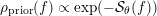 $\unicode[STIX]{x1D70C}_{\text{prior}}(f)\propto \exp (-{\mathcal{S}}_{\unicode[STIX]{x1D703}}(f))$
(Kaipio and Somersalo Reference Kaipio and Somersalo2005) where
$\unicode[STIX]{x1D70C}_{\text{prior}}(f)\propto \exp (-{\mathcal{S}}_{\unicode[STIX]{x1D703}}(f))$
(Kaipio and Somersalo Reference Kaipio and Somersalo2005) where
 $\unicode[STIX]{x1D70C}_{\text{prior}}$
is the density for the prior. The situation is more complicated in the infinite-dimensional setting since a MAP estimator does not always exist, and if it exists then there is no general scheme for connecting the topological description of a MAP estimate to a variational problem. The main reason is that the posterior no longer has a natural density representation, which significantly complicates the definition and study of the underlying conditional probabilities.
$\unicode[STIX]{x1D70C}_{\text{prior}}$
is the density for the prior. The situation is more complicated in the infinite-dimensional setting since a MAP estimator does not always exist, and if it exists then there is no general scheme for connecting the topological description of a MAP estimate to a variational problem. The main reason is that the posterior no longer has a natural density representation, which significantly complicates the definition and study of the underlying conditional probabilities.
Assume the prior measure is specified by a Gaussian random field, and the likelihood satisfies conditions in Theorem 3.9 that are necessary for the existence of a well-posed posterior measure. Then the MAP estimator is well-defined as the minimizer of an Onsager–Machlup functional defined on the Cameron–Martin space of the prior. If one has Gaussian noise, then this becomes a least-squares functional penalized by a regularization functional that is the Cameron–Martin norm of the Gaussian prior (Dashti et al. Reference Dashti, Law, Stuart and Voss2013); see also Dashti and Stuart (Reference Dashti, Stuart and Ghanem2017, Section 4.3). To handle the case with non-Gaussian priors, Helin and Burger (Reference Helin and Burger2015) introduce the notion of weak MAP estimate (wMAP) and show that a wMAP estimate can be connected to a variational formulation also for non-Gaussian priors. Furthermore, any MAP estimate in the sense of Dashti et al. (Reference Dashti, Law, Stuart and Voss2013) is a wMAP estimate, so this is a generalization in the strict sense. The wMAP approach, however, fails when the prior does not admit continuous densities. In order to handle this, Clason, Helin, Kretschmann and Piiroinen (Reference Clason, Helin, Kretschmann and Piiroinen2018) introduce the notion of a generalized mode of a probability measure (Clason et al. Reference Clason, Helin, Kretschmann and Piiroinen2018, Definition 2.3) and define a (generalized) MAP estimator as a generalized mode of the posterior measure. Generalized MAP reduces to the classical MAP in certain situations that include Gaussian priors but the former also exist for a more general class of priors, such as uniform priors. The main result in Clason et al. (Reference Clason, Helin, Kretschmann and Piiroinen2018) is that one can characterize a generalized MAP estimator as a minimizer of an Onsager–Machlup functional even in cases when the prior does not admit a continuous density.
As a final remark, while a MAP estimate with a Gaussian noise model does lead to an optimization problem with a quadratic data-fidelity term, Gribonval and Nikolova (Reference Gribonval and Nikolova2018) show via explicit examples that the converse is not true. They characterize those data models of the type in (3.2) where Bayes estimators can be expressed as the solution of a penalized least-squares optimization problem. One example is denoising in the presence of additive Gaussian noise and an arbitrary prior; another is a data model with (a variant of) Poisson noise and any prior probability on the unknowns. In these cases, the variational approach is rich enough to build all possible Bayes estimators via a well-chosen penalty.
3.4 Explicit priors
The choice of prior is important in Bayesian inversion, and much of the work has focused on characterizing families of priors that ensure posterior consistency holds and for which there are good convergence rates (Section 3.2.3).
From the general Bayesian statistics literature, much effort has gone into characterizing robust priors. These have limited influence (in the asymptotic regime) on the posterior (Bayesian robustness), and such non-informative priors are useful for Bayesian inversion when there is not enough information to choose a prior for the unknown model parameter, or when the information available is not easily translated into a probabilistic statement: see Berger (Reference Berger1985, Section 4.7.9) and Calvetti and Somersalo (Reference Calvetti and Somersalo2017). For example, hierarchical priors tend to be robust (Berger Reference Berger1985, Section 4.7.9). Another class is that of conjugate priors, which are desirable from a computational perspective (Section 3.5.2) since they have tails that are typically of the same form as the likelihood function. Conjugate priors also remain influential when the likelihood function is concentrated in the (prior) tail, so natural conjugate priors are therefore not necessarily robust (Berger Reference Berger1985, Section 4.7).
Priors on digitized images.
A wide range of priors for Bayesian inversion have been suggested when the unknown model parameter represents a digitized image, the latter given by a real-valued function in some suitable class defined on a domain
 $\unicode[STIX]{x1D6FA}\subset \mathbb{R}^{n}$
.
$\unicode[STIX]{x1D6FA}\subset \mathbb{R}^{n}$
.
One such class is that of smoothness priors, which reflect the belief that values of the model parameter at a point are close to the average of its values in a neighbourhood of that point. Another is structural priors, which allow for more abrupt (discontinuous) changes in the values of the unknown model parameter at specific locations. Yet another is sparsity-promoting priors (see Section 2.7), which encode the a priori belief that the unknown model parameter is compressible with respect to some underlying dictionary, that is, it can be transformed into a linear combination of dictionary elements where most coefficients vanish (or are small). Finally, there are hierarchical priors which are formed by combining other priors hierarchically into an overall prior. This is typically done in a two-step process where one first specifies some underlying priors, often taken as natural conjugate priors, and then mixes them in a second stage over hyper-parameters. Recently, Calvetti, Somersalo and Strang (Reference Calvetti, Somersalo and Strang2019) have reformulated the question of sparse recovery as an inverse problem in the Bayesian framework, and expressed the sparsity criteria by means of a hierarchical prior mode. More information and further examples of priors in the finite-dimensional setting are given by Kaipio and Somersalo (Reference Kaipio and Somersalo2005), Calvetti and Somersalo (Reference Calvetti and Somersalo2008, Reference Calvetti and Somersalo2017) and Calvetti et al. (Reference Calvetti, Somersalo and Strang2019).
Priors on function spaces.
Defining priors when
 $X$
is an infinite-dimensional function space is somewhat involved. A common approach is to consider a convergent series expansion and then let the coefficients be generated by a random variable.
$X$
is an infinite-dimensional function space is somewhat involved. A common approach is to consider a convergent series expansion and then let the coefficients be generated by a random variable.
More precisely, consider the case when
 $X$
is a Banach space of real-valued functions on some fixed domain
$X$
is a Banach space of real-valued functions on some fixed domain
 $\unicode[STIX]{x1D6FA}\subset \mathbb{R}^{d}$
. Following Dashti and Stuart (Reference Dashti, Stuart and Ghanem2017, Section 2.1), let
$\unicode[STIX]{x1D6FA}\subset \mathbb{R}^{d}$
. Following Dashti and Stuart (Reference Dashti, Stuart and Ghanem2017, Section 2.1), let
 $\{{\unicode[STIX]{x1D719}_{i}\}}_{i}\subset X$
be a countable sequence whose elements are normalized, i.e.
$\{{\unicode[STIX]{x1D719}_{i}\}}_{i}\subset X$
be a countable sequence whose elements are normalized, i.e.
 $\Vert \unicode[STIX]{x1D719}_{i}\Vert _{X}=1$
. Now consider model parameters
$\Vert \unicode[STIX]{x1D719}_{i}\Vert _{X}=1$
. Now consider model parameters
 $f\in X$
of the form
$f\in X$
of the form
 $$\begin{eqnarray}f=f_{0}+\mathop{\sum }_{i}\unicode[STIX]{x1D6FC}_{i}\unicode[STIX]{x1D719}_{i},\end{eqnarray}$$
where
 $f_{0}\in X$
is not necessarily normalized to 1. A probability distribution on the coefficients
$f_{0}\in X$
is not necessarily normalized to 1. A probability distribution on the coefficients
 $\unicode[STIX]{x1D6FC}_{i}$
renders a real-valued random function on
$\unicode[STIX]{x1D6FC}_{i}$
renders a real-valued random function on
 $\unicode[STIX]{x1D6FA}$
: simply define the deterministic sequence
$\unicode[STIX]{x1D6FA}$
: simply define the deterministic sequence
 $\{{\unicode[STIX]{x1D6FE}_{i}\}}_{i}\subset \mathbb{R}$
and the i.i.d. random sequence
$\{{\unicode[STIX]{x1D6FE}_{i}\}}_{i}\subset \mathbb{R}$
and the i.i.d. random sequence
 $\{{\unicode[STIX]{x1D709}_{i}\}}_{i}\subset \mathbb{R}$
and set
$\{{\unicode[STIX]{x1D709}_{i}\}}_{i}\subset \mathbb{R}$
and set
 $\unicode[STIX]{x1D6FC}_{i}=\unicode[STIX]{x1D6FE}_{i}\unicode[STIX]{x1D709}_{i}$
. This generates a probability measure
$\unicode[STIX]{x1D6FC}_{i}=\unicode[STIX]{x1D6FE}_{i}\unicode[STIX]{x1D709}_{i}$
. This generates a probability measure
 $\unicode[STIX]{x1D6F1}_{\text{prior}}$
on
$\unicode[STIX]{x1D6F1}_{\text{prior}}$
on
 $X$
by taking the pushforward of the measure on the i.i.d. random sequence
$X$
by taking the pushforward of the measure on the i.i.d. random sequence
 $\{{\unicode[STIX]{x1D709}_{i}\}}_{i}\subset \mathbb{R}$
under the map which takes the sequence into the random function.
$\{{\unicode[STIX]{x1D709}_{i}\}}_{i}\subset \mathbb{R}$
under the map which takes the sequence into the random function.
Using the above technique, one can construct a uniform prior that can be shown to generate random functions that are all contained in a subset
 $X\subset L^{\infty }(\unicode[STIX]{x1D6FA})$
, which can be characterized (Dashti and Stuart Reference Dashti, Stuart and Ghanem2017, Theorem 2). It is likewise possible to define Gaussian priors where the random function exists as an
$X\subset L^{\infty }(\unicode[STIX]{x1D6FA})$
, which can be characterized (Dashti and Stuart Reference Dashti, Stuart and Ghanem2017, Theorem 2). It is likewise possible to define Gaussian priors where the random function exists as an
 $L^{2}$
limit in Sobolev spaces of sufficient smoothness (Dashti and Stuart Reference Dashti, Stuart and Ghanem2017, Theorem 8). For imaging applications, much effort has been devoted to constructing edge-preserving priors. An obvious candidate is the TV-prior, but it is not ‘discretization-invariant’ as its edge-preserving property is lost when the discretization becomes finer. This prompted the development of other edge-preserving priors, such as Besov space priors, which are discretization-invariant (Lassas et al.
Reference Lassas, Saksman and Siltanen2009, Kolehmainen, Lassas, Niinimäki and Siltanen Reference Kolehmainen, Lassas, Niinimäki and Siltanen2012). See also Dashti and Stuart (Reference Dashti, Stuart and Ghanem2017, Theorem 5), which characterizes Besov priors that generate random functions contained in separable Banach spaces. However, edge-preserving inversion using a Besov space prior often relies on the Haar wavelet basis. Due to the structure of the Haar basis, discontinuities are preferred on an underlying dyadic grid given by the discontinuities of the basis functions. As an example, on
$L^{2}$
limit in Sobolev spaces of sufficient smoothness (Dashti and Stuart Reference Dashti, Stuart and Ghanem2017, Theorem 8). For imaging applications, much effort has been devoted to constructing edge-preserving priors. An obvious candidate is the TV-prior, but it is not ‘discretization-invariant’ as its edge-preserving property is lost when the discretization becomes finer. This prompted the development of other edge-preserving priors, such as Besov space priors, which are discretization-invariant (Lassas et al.
Reference Lassas, Saksman and Siltanen2009, Kolehmainen, Lassas, Niinimäki and Siltanen Reference Kolehmainen, Lassas, Niinimäki and Siltanen2012). See also Dashti and Stuart (Reference Dashti, Stuart and Ghanem2017, Theorem 5), which characterizes Besov priors that generate random functions contained in separable Banach spaces. However, edge-preserving inversion using a Besov space prior often relies on the Haar wavelet basis. Due to the structure of the Haar basis, discontinuities are preferred on an underlying dyadic grid given by the discontinuities of the basis functions. As an example, on
 $[0,1]$
a Besov space prior prefers a discontinuity at
$[0,1]$
a Besov space prior prefers a discontinuity at
 $x=1/4$
over
$x=1/4$
over
 $x=1/3$
. Thus, in most practical cases, Besov priors rely on both a strong and unrealistic assumption. For this reason, Markkanen, Roininen, Huttunen and Lasanen (Reference Markkanen, Roininen, Huttunen and Lasanen2019) propose another class of priors for edge-preserving Bayesian inversion, the Cauchy difference priors. Starting from continuous one-dimensional Cauchy motion, its discretized version, Cauchy random walk, can be used as a non-Gaussian prior for edge-preserving Bayesian inversion. As shown by Markkanen et al. (Reference Markkanen, Roininen, Huttunen and Lasanen2019), one can also develop a suitable posterior distribution sampling algorithm for computing the conditional mean estimates with single-component Metropolis–Hastings. The approach is applied to CT reconstruction problems in materials science.
$x=1/3$
. Thus, in most practical cases, Besov priors rely on both a strong and unrealistic assumption. For this reason, Markkanen, Roininen, Huttunen and Lasanen (Reference Markkanen, Roininen, Huttunen and Lasanen2019) propose another class of priors for edge-preserving Bayesian inversion, the Cauchy difference priors. Starting from continuous one-dimensional Cauchy motion, its discretized version, Cauchy random walk, can be used as a non-Gaussian prior for edge-preserving Bayesian inversion. As shown by Markkanen et al. (Reference Markkanen, Roininen, Huttunen and Lasanen2019), one can also develop a suitable posterior distribution sampling algorithm for computing the conditional mean estimates with single-component Metropolis–Hastings. The approach is applied to CT reconstruction problems in materials science.
The above constructions of random functions through randomized series can be linked to each other through the notion of random fields as shown in Dashti and Stuart (Reference Dashti, Stuart and Ghanem2017, Section 2.5); see also Ghosal and van der Vaart (Reference Ghosal and van der Vaart2017, Chapters 2 and 10) for further examples. These constructions also extend straightforwardly to
 $\mathbb{R}^{n}$
- or
$\mathbb{R}^{n}$
- or
 $\mathbb{C}^{n}$
-valued functions.
$\mathbb{C}^{n}$
-valued functions.
3.5 Challenges
The statistical view of an inverse problem in Bayesian inversion extends the functional analytic one, since the output is ideally the posterior that describes all possible solutions. This is very tractable and fits well within the scientific tradition of presenting data and inferred quantities with error bars.
Most priors are chosen to regularize the problem rather than improving the output quality. Next, algorithmic advances (Section 3.5.2) have resulted in methods that can sample in a computationally feasible manner from a posterior distribution in a high-dimensional setting, say up to
 $10^{6}$
dimensions. This is still not sufficient for large-scale two-dimensional imaging or regular three-dimensional imaging applications. Furthermore, these methods require an explicit prior, which may not be feasible if one uses learning to obtain it. They may also make use of analytic approximations such as those given in Section 3.2.5, which restricts the priors that can come into question. For these reasons, most applications of Bayesian inversion on large-scale problems only compute a MAP estimator, whereas estimators requiring integration over the model parameter space remain computationally unfeasible. These include Bayes estimators and the conditional mean as well as estimators relevant for uncertainty quantification.
$10^{6}$
dimensions. This is still not sufficient for large-scale two-dimensional imaging or regular three-dimensional imaging applications. Furthermore, these methods require an explicit prior, which may not be feasible if one uses learning to obtain it. They may also make use of analytic approximations such as those given in Section 3.2.5, which restricts the priors that can come into question. For these reasons, most applications of Bayesian inversion on large-scale problems only compute a MAP estimator, whereas estimators requiring integration over the model parameter space remain computationally unfeasible. These include Bayes estimators and the conditional mean as well as estimators relevant for uncertainty quantification.
In conclusion, the above difficulties in specifying a ‘good’ prior and in meeting the computational requirements have seriously limited the dissemination of Bayes inversion in large-scale inverse problems, such as those arising in imaging. Before providing further remarks on this, let us mention that Section 5.1 shows how techniques from deep learning can be used to address the above challenges when computing a wide range of estimators. Likewise, in Section 5.2 we show how deep learning can be used to efficiently sample from the posterior.
3.5.1 Choosing a good prior
Current theory for choosing a ‘good’ prior mainly emphasizes the regularizing function of the prior (Section 3.4). In particular, one seeks a prior that ensures posterior consistency (Section 3.2.3) and good contraction rates (Section 3.2.4) and, if possible, also allows for an asymptotic characterization of the posterior (Section 3.2.5).
This theory, however, is for the asymptotic setting as the noise level in data tends to zero, whereas there seems to be no theory for Bayesian inversion that deals with the setting when the data have a fixed noise level. Here, the prior has a role that goes beyond acting as a regularizer, and its choice may have a large influence on the posterior. For example, it is far from clear whether a prior that provides ‘optimal’ contraction rates is the most suitable one when the data are fixed with a given noise level. Another difficulty is that norms used to quantify distance in the mathematical theorems have little to do with what is meant by a ‘good’ estimate of a model parameter. An archetypal example is the difficulty in quantifying the notion of ‘image quality’ in radiology. This is very difficult since the notion of image quality depends on the task motivating the imaging application. Hand-crafted priors surveyed in Section 3.4 have limitations in this regard, and in Sections 4.3, 4.4, 4.7 and 4.10 we survey work that uses data-driven modelling to obtain a prior.
3.5.2 Computational feasibility
The focus here is on techniques that are not based on deep learning for sampling from a very high-dimensional posterior distribution that lacks an explicit expression.
A well-known class of methods is based on Markov chain Monte Carlo (MCMC), where the aim is to define an iterative process whose stationary distribution coincides with the target distribution, which in Bayesian inversion is the posterior. MCMC techniques come in many variants, and one common variant is MCMC sampling with Metropolis–Hastings dynamics (Minh and Le Minh Reference Minh and Le Minh2015), which generates a Markov chain with equilibrium distribution that coincides with the posterior in the limit. Other variants use Gibbs sampling, which reduces the autocorrelation between samples. Technically, Gibbs sampling can be seen as a special case of Metropolis–Hastings dynamics and it requires computation of conditional distributions. Further variants are auxiliary variable MCMC methods, such as slice sampling (Neal Reference Neal2003), proximal MCMC (Green, Łatuszysński, Pereyra and Robert Reference Green, Łatuszysński, Pereyra and Robert2015, Durmus, Moulines and Pereyra Reference Durmus, Moulines and Pereyra2018, Repetti, Pereyra and Wiaux Reference Repetti, Pereyra and Wiaux2019) and Hamiltonian Monte Carlo (Girolami and Calderhead Reference Girolami and Calderhead2011, Betancourt Reference Betancourt2017). See also Dashti and Stuart (Reference Dashti, Stuart and Ghanem2017, Section 5) for a nice abstract description of MCMC in the context of infinite-dimensional Bayesian inversion.
An alternative approach to MCMC seeks to approximate the posterior with more tractable distributions (deterministic inference), for example in variational Bayes inference (Fox and Roberts Reference Fox and Roberts2012, Blei, Küçükelbir and McAuliffe Reference Blei, Küçükelbir and McAuliffe2017) and expectation propagation (Minka Reference Minka, Breese and Koller2001). Variational Bayes inference has indeed emerged as a popular alternative to the classical MCMC methods for sampling from a difficult-to-compute probability distribution, which in Bayesian inversion is the posterior distribution. The idea is to start from a fixed family of probability distributions (variational family) and select the one that best approximates the target distribution under some similarity measure, such as the Kullback–Leibler divergence.
Blei et al. (Reference Blei, Küçükelbir and McAuliffe2017, p. 860) try to provide some guidance on when to use MCMC and when to use variational Bayes. MCMC methods tend to be more computationally intensive than variational inference, but they also provide guarantees of producing (asymptotically) exact samples from the target density (Robert and Casella Reference Robert and Casella2004). Variational inference does not enjoy such guarantees: it can only find a density close to the target but tends to be faster than MCMC. A recent development is the proof of a Bernstein–von Mises theorem (Wang and Blei Reference Wang and Blei2017, Theorem 5), which shows that the variational Bayes posterior is asymptotically normal around the variational frequentist estimate. Hence, if the variational frequentist estimate is consistent, then the variational Bayes posterior converges to a Gaussian with a mean centred at the true model parameter. Furthermore, since variational Bayes rests on optimization, variational inference easily takes advantage of methods such as stochastic optimization (Robbins and Monro Reference Robbins and Monro1951, Kushner and Yin Reference Kushner and Yin1997) and distributed optimization (though some MCMC methods can also exploit these innovations (Welling and Teh Reference Welling and Teh2011, Ahmed et al. Reference Ahmed, Aly, Gonzalez, Narayanamurthy and Smola2012)). Thus, variational inference is suited to large data sets and scenarios where we want to quickly explore many models; MCMC is suited to smaller data sets and scenarios where we are happy to pay a heavier computational cost for more precise samples. Another factor is the geometry of the posterior distribution. For example, the posterior of a mixture model admits multiple modes, each corresponding to label permutations of the components. Gibbs sampling, if the model permits, is a powerful approach to sampling from such target distributions; it quickly focuses on one of the modes. For mixture models where Gibbs sampling is not an option, variational inference may perform better than a more general MCMC technique (e.g. Hamiltonian Monte Carlo), even for small datasets (Küçükelbir, Ranganath, Gelman and Blei Reference Küçükelbir, Ranganath, Gelman and Blei2017).
4 Learning in functional analytic regularization
There have been two main ways to incorporate learning into functional analytic regularization. The first relates to the ‘evolution’ of regularizing functionals, primarily within variational regularization (Sections 4.3, 4.4, 4.6, 4.7 and 4.10). Early approaches focused on using measured data to determine the regularization parameter(s), but as prior models became increasingly complex, this blended into approaches where one learns a highly parametrized regularizer from data. The second category uses learning to address the computational challenge associated with variational regularization. The idea is to ‘learn how to optimize’ in variational regularization given an a priori bound on the computational budget (Section 4.9).
4.1 Choosing the regularization parameter
To introduce this topic we first consider the simplified case where only one parameter is used for characterizing the scale of regularization as in (2.10) and in the functional analytic regularization methods encountered in Sections 2.5–2.7. Thus we use the notation of Remarks 2.3 and 2.6, that is,
 $f_{\text{true}}$
denotes the true (unknown) model parameter and
$f_{\text{true}}$
denotes the true (unknown) model parameter and
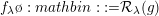 $f_{\unicode[STIX]{x1D706}} :={\mathcal{R}}_{\unicode[STIX]{x1D706}}(g)$
is the regularized solution obtained from applying a reconstruction operator
$f_{\unicode[STIX]{x1D706}} :={\mathcal{R}}_{\unicode[STIX]{x1D706}}(g)$
is the regularized solution obtained from applying a reconstruction operator
 ${\mathcal{R}}_{\unicode[STIX]{x1D706}}:Y\rightarrow X$
on data
${\mathcal{R}}_{\unicode[STIX]{x1D706}}:Y\rightarrow X$
on data
 $g$
satisfying (2.1).
$g$
satisfying (2.1).
In this context, and recalling some historical classification, the three main types of parameter choice rules are characterized as a posteriori, a priori and error-free parameter choice rules: see Bertero and Boccacci (Reference Bertero and Boccacci1998, Section 5.6) and Engl et al. (Reference Engl, Hanke and Neubauer2000). With hindsight, many of these parameter choice rules can be seen as early attempts to use ‘learning’ from data in the context of reconstruction.
A posteriori rules. This class of rules is based on the assumption that a reasonably tight estimate of the data discrepancy and/or value of regularizer at the true solution can be accessed. That is, one knows
 $\unicode[STIX]{x1D716}>0$
and/or
$\unicode[STIX]{x1D716}>0$
and/or
 $S>0$
such that
$S>0$
such that
 $$\begin{eqnarray}{\mathcal{L}}({\mathcal{A}}(f_{\text{true}}),g)\leq \unicode[STIX]{x1D716}\text{for }g={\mathcal{A}}(f_{\text{true}})+e\quad \text{and/or}\quad {\mathcal{S}}(f_{\text{true}})\leq S.\end{eqnarray}$$
A prominent example of an a posteriori parameter choice rule is the Morozov discrepancy principle (Morozov Reference Morozov1966). Here, the regularization parameter
 $\unicode[STIX]{x1D706}$
is chosen so that
$\unicode[STIX]{x1D706}$
is chosen so that
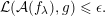 $$\begin{eqnarray}{\mathcal{L}}({\mathcal{A}}(f_{\unicode[STIX]{x1D706}}),g)\leq \unicode[STIX]{x1D716}.\end{eqnarray}$$
Another example is Miller’s method (Miller Reference Miller1970), where the regularization parameter
 $\unicode[STIX]{x1D706}$
is chosen so that
$\unicode[STIX]{x1D706}$
is chosen so that
 $$\begin{eqnarray}{\mathcal{L}}({\mathcal{A}}(f_{\unicode[STIX]{x1D706}}),g)\leq \unicode[STIX]{x1D716}\quad \text{and}\quad {\mathcal{S}}(f_{\unicode[STIX]{x1D706}})\leq S.\end{eqnarray}$$
A priori rules. These methods combine an estimate of the noise level in the data with some knowledge of the smoothness of the solution as a priori information. Hence, the choice of regularization parameter can be made before computing
 $f_{\unicode[STIX]{x1D706}}$
. The choice of
$f_{\unicode[STIX]{x1D706}}$
. The choice of
 $\unicode[STIX]{x1D706}$
is ideally guided by a theorem that ensures the parameter choice rule yields an optimal convergence rate, for example as in Theorem 2.7 where the (scalar) regularization parameter is chosen in proportion to the noise level. For more detailed references, see Engl et al. (Reference Engl, Hanke and Neubauer2000) and Kindermann (Reference Kindermann2011).
$\unicode[STIX]{x1D706}$
is ideally guided by a theorem that ensures the parameter choice rule yields an optimal convergence rate, for example as in Theorem 2.7 where the (scalar) regularization parameter is chosen in proportion to the noise level. For more detailed references, see Engl et al. (Reference Engl, Hanke and Neubauer2000) and Kindermann (Reference Kindermann2011).
Error-free parameter choice rules. Use data to guide the choice of parameter, for example by balancing principles between the error in the fidelity and the regularization terms. An important example in this context is generalized cross-validation (Golub, Heat and Wahba Reference Golub, Heat and Wahba1979). Let
 $f_{\unicode[STIX]{x1D706}}^{[k]}\in X$
denote the regularized solution obtained from data when we have removed the
$f_{\unicode[STIX]{x1D706}}^{[k]}\in X$
denote the regularized solution obtained from data when we have removed the
 $k$
th component
$k$
th component
 $g_{k}$
of
$g_{k}$
of
 $g$
. Then the regularization parameter
$g$
. Then the regularization parameter
 $\unicode[STIX]{x1D706}$
is chosen to predict the missing data values:
$\unicode[STIX]{x1D706}$
is chosen to predict the missing data values:
 $$\begin{eqnarray}\text{minimize }\unicode[STIX]{x1D706}\mapsto \mathop{\sum }_{k=1}^{m}|{\mathcal{A}}(f_{\unicode[STIX]{x1D706}}^{[k]})_{k}-g_{k}|\quad \text{subject to }{\mathcal{A}}(f_{\unicode[STIX]{x1D706}}^{[k]})_{k}\simeq g_{k}.\end{eqnarray}$$
Another method within this class is the L-curve (Hansen Reference Hansen1992). Here the regularization parameter
 $\unicode[STIX]{x1D706}$
is chosen where the log-log plot of
$\unicode[STIX]{x1D706}$
is chosen where the log-log plot of
 $\unicode[STIX]{x1D706}\mapsto ({\mathcal{L}}({\mathcal{A}}(f_{\unicode[STIX]{x1D706}}),g)+\unicode[STIX]{x1D706}{\mathcal{S}}(f_{\unicode[STIX]{x1D706}}))$
has the highest curvature (i.e. it exhibits a corner).
$\unicode[STIX]{x1D706}\mapsto ({\mathcal{L}}({\mathcal{A}}(f_{\unicode[STIX]{x1D706}}),g)+\unicode[STIX]{x1D706}{\mathcal{S}}(f_{\unicode[STIX]{x1D706}}))$
has the highest curvature (i.e. it exhibits a corner).
Most of the work on parameter choice techniques addresses the case of a single scalar parameter. Much of the theory is developed for additive Gaussian noise, that is, when the data discrepancy
 ${\mathcal{L}}$
is a squared (possibly weighted) 2-norm. For error-free parameter choice rules, convergence
${\mathcal{L}}$
is a squared (possibly weighted) 2-norm. For error-free parameter choice rules, convergence
 $f_{\unicode[STIX]{x1D706}(\unicode[STIX]{x1D6FF})}\rightarrow f_{\text{true}}$
as
$f_{\unicode[STIX]{x1D706}(\unicode[STIX]{x1D6FF})}\rightarrow f_{\text{true}}$
as
 $\unicode[STIX]{x1D6FF}\rightarrow 0$
cannot be guaranteed (Bakushinskii Reference Bakushinskii1984). Error-free parameter choice rules are computationally very demanding as they require solutions for varying values of the regularization parameter. Although many rules have been proposed, very few of them are used in practice. In Section 4.3.1 we will encounter another instance of parameter choice rules for TV-type regularization problems via bilevel learning.
$\unicode[STIX]{x1D6FF}\rightarrow 0$
cannot be guaranteed (Bakushinskii Reference Bakushinskii1984). Error-free parameter choice rules are computationally very demanding as they require solutions for varying values of the regularization parameter. Although many rules have been proposed, very few of them are used in practice. In Section 4.3.1 we will encounter another instance of parameter choice rules for TV-type regularization problems via bilevel learning.
4.2 Learning in approximate analytic inversion
Early approaches to using learning in approximate analytic inversion (Section 2.4) mostly dealt with the FBP method for tomographic image reconstruction.
One of the first examples of the above is that of Floyd (Reference Floyd1991), which learns the reconstruction filter of an analytic reconstruction algorithm. The same principle is considered by Würfl et al. (Reference Würfl, Hoffmann, Christlein, Breininger, Huang, Unberath and Maier2018), who have designed a convolutional neural network (CNN) architecture specifically adapted to encode an analytic reconstruction algorithm for inverting the ray transform. A key observation is that the normal operator
 ${\mathcal{A}}^{\ast }{\mathcal{A}}$
is of convolutional type when
${\mathcal{A}}^{\ast }{\mathcal{A}}$
is of convolutional type when
 ${\mathcal{A}}$
is the ray transform, and the reconstruction filter in FBP acts by a convolution as well. Hence, both of these are easily representable in a CNN. The paper gives explicit constructions of such partial differential equations (CNNs) for FBP in parallel-beam geometry and fan-beam geometry and the Feldkamp–Davis–Kress method in cone-beam geometry. Having the analytic reconstruction operator encoded as a CNN allows one to learn every other possible step in it, so the approach in Würfl et al. (Reference Würfl, Hoffmann, Christlein, Breininger, Huang, Unberath and Maier2018) actually goes beyond learning the reconstruction filter of an analytic reconstruction algorithm. Finally, we mention Janssens et al. (Reference Janssens, Beenhouwer, Dael, Schryver, Hoorebeke, Verboven, Nicolai and Sijbers2018), who consider a fan-beam reconstruction algorithm based on the Hilbert transform FBP (You and Zeng Reference You and Zeng2007) for which the filter is trained by a neural network.
${\mathcal{A}}$
is the ray transform, and the reconstruction filter in FBP acts by a convolution as well. Hence, both of these are easily representable in a CNN. The paper gives explicit constructions of such partial differential equations (CNNs) for FBP in parallel-beam geometry and fan-beam geometry and the Feldkamp–Davis–Kress method in cone-beam geometry. Having the analytic reconstruction operator encoded as a CNN allows one to learn every other possible step in it, so the approach in Würfl et al. (Reference Würfl, Hoffmann, Christlein, Breininger, Huang, Unberath and Maier2018) actually goes beyond learning the reconstruction filter of an analytic reconstruction algorithm. Finally, we mention Janssens et al. (Reference Janssens, Beenhouwer, Dael, Schryver, Hoorebeke, Verboven, Nicolai and Sijbers2018), who consider a fan-beam reconstruction algorithm based on the Hilbert transform FBP (You and Zeng Reference You and Zeng2007) for which the filter is trained by a neural network.
4.3 Bilevel optimization
In variational methods (see Section 2.6), we define the reconstruction operator
 ${\mathcal{R}}_{\unicode[STIX]{x1D703}}:Y\rightarrow X$
by
${\mathcal{R}}_{\unicode[STIX]{x1D703}}:Y\rightarrow X$
by
As already mentioned, ideally
 $f\mapsto {\mathcal{L}}({\mathcal{A}}(f),g)$
corresponds to an affine transformation of the negative log-likelihood of the data. However, it is less clear how to choose the regularizer
$f\mapsto {\mathcal{L}}({\mathcal{A}}(f),g)$
corresponds to an affine transformation of the negative log-likelihood of the data. However, it is less clear how to choose the regularizer
 ${\mathcal{S}}_{\unicode[STIX]{x1D703}}:X\rightarrow \mathbb{R}$
and/or the value for the parameter
${\mathcal{S}}_{\unicode[STIX]{x1D703}}:X\rightarrow \mathbb{R}$
and/or the value for the parameter
 $\unicode[STIX]{x1D703}$
.
$\unicode[STIX]{x1D703}$
.
The focus here is on formulating a generic set-up for learning selected components of (4.2) from supervised training data given a loss function
 $\ell _{X}:X\times X\rightarrow \mathbb{R}$
. This set-up can be tailored towards learning the regularization functional
$\ell _{X}:X\times X\rightarrow \mathbb{R}$
. This set-up can be tailored towards learning the regularization functional
 ${\mathcal{S}}$
, or the data fidelity term
${\mathcal{S}}$
, or the data fidelity term
 ${\mathcal{L}}$
, or an appropriate component in a forward operator
${\mathcal{L}}$
, or an appropriate component in a forward operator
 ${\mathcal{A}}$
, e.g. in blind image deconvolution (Hintermüller and Wu Reference Hintermüller and Wu2015). The starting point is to have access to supervised training data
${\mathcal{A}}$
, e.g. in blind image deconvolution (Hintermüller and Wu Reference Hintermüller and Wu2015). The starting point is to have access to supervised training data
 $(f_{i},g_{i})\in X\times Y$
that are generated by a
$(f_{i},g_{i})\in X\times Y$
that are generated by a
 $(X\times Y)$
-valued random variable
$(X\times Y)$
-valued random variable
 $(\unicode[STIX]{x1D557},\unicode[STIX]{x1D558})\sim \unicode[STIX]{x1D707}$
. We can then form the following bilevel optimization formulation:
$(\unicode[STIX]{x1D557},\unicode[STIX]{x1D558})\sim \unicode[STIX]{x1D707}$
. We can then form the following bilevel optimization formulation:
Note here that
 $\widehat{\unicode[STIX]{x1D703}}$
is a Bayes estimator, but
$\widehat{\unicode[STIX]{x1D703}}$
is a Bayes estimator, but
 $\unicode[STIX]{x1D707}$
is not fully known. Instead it is replaced by its empirical counterpart given by the supervised training data, in which case
$\unicode[STIX]{x1D707}$
is not fully known. Instead it is replaced by its empirical counterpart given by the supervised training data, in which case
 $\widehat{\unicode[STIX]{x1D703}}$
corresponds to empirical risk minimization Section 3.3.
$\widehat{\unicode[STIX]{x1D703}}$
corresponds to empirical risk minimization Section 3.3.
In the bilevel optimization literature, as in the optimization literature as a whole, there are two main and mostly distinct approaches. The first one is the discrete approach that first discretizes the problem (4.2) and subsequently optimizes its parameters. In this way, optimality conditions and their well-posedness are derived in finite dimensions, which circumvents often difficult topological considerations related to convergence in infinite-dimensional function spaces, but also jeopardizes preservation of continuous structure (i.e. optimizing the discrete problem is not automatically equivalent to discretizing the optimality conditions of the continuous problem (De los Reyes Reference De los Reyes2015)) and dimension-invariant convergence properties.
Alternatively, (4.2) and its parameter
 $\unicode[STIX]{x1D703}$
are optimized in the continuum (i.e. appropriate infinite-dimensional function spaces) and then discretized. The resulting problems present several difficulties due to the frequent non-smoothness of the lower-level problem (think of TV regularization), which, in general, makes it impossible to verify Karush–Kuhn–Tucker constraint qualification conditions. This issue has led to the development of alternative analytical approaches in order to obtain first-order necessary optimality conditions (Bonnans and Tiba Reference Bonnans and Tiba1991, De los Reyes Reference De los Reyes2011, Hintermüller, Laurain, Löbhard, Rautenberg and Surowiec Reference Hintermüller, Laurain, Löbhard, Rautenberg, Surowiec and Leugering2014). The bilevel problems under consideration are also related to generalized mathematical programs with equilibrium constraints in function spaces (Luo, Pang and Ralph Reference Luo, Pang and Ralph1996, Outrata Reference Outrata2000).
$\unicode[STIX]{x1D703}$
are optimized in the continuum (i.e. appropriate infinite-dimensional function spaces) and then discretized. The resulting problems present several difficulties due to the frequent non-smoothness of the lower-level problem (think of TV regularization), which, in general, makes it impossible to verify Karush–Kuhn–Tucker constraint qualification conditions. This issue has led to the development of alternative analytical approaches in order to obtain first-order necessary optimality conditions (Bonnans and Tiba Reference Bonnans and Tiba1991, De los Reyes Reference De los Reyes2011, Hintermüller, Laurain, Löbhard, Rautenberg and Surowiec Reference Hintermüller, Laurain, Löbhard, Rautenberg, Surowiec and Leugering2014). The bilevel problems under consideration are also related to generalized mathematical programs with equilibrium constraints in function spaces (Luo, Pang and Ralph Reference Luo, Pang and Ralph1996, Outrata Reference Outrata2000).
One of the first examples of the above is the paper by Haber and Tenorio (Reference Haber and Tenorio2003), who considered a regularization functional
 ${\mathcal{S}}_{\unicode[STIX]{x1D703}}:X\rightarrow \mathbb{R}$
that can depend on location and involves derivatives or other filters. Concrete examples are anisotropic weighted Dirichlet energy where
${\mathcal{S}}_{\unicode[STIX]{x1D703}}:X\rightarrow \mathbb{R}$
that can depend on location and involves derivatives or other filters. Concrete examples are anisotropic weighted Dirichlet energy where
 $\unicode[STIX]{x1D703}$
is a function, that is,
$\unicode[STIX]{x1D703}$
is a function, that is,
 $$\begin{eqnarray}{\mathcal{S}}_{\unicode[STIX]{x1D703}}(f):=\Vert \unicode[STIX]{x1D703}(\,\cdot \,)\unicode[STIX]{x1D6FB}f(\,\cdot \,)\Vert _{2}^{2}\quad \text{for }\unicode[STIX]{x1D703}:\unicode[STIX]{x1D6FA}\rightarrow \mathbb{R},\end{eqnarray}$$
and anisotropic weighted TV,
 $$\begin{eqnarray}{\mathcal{S}}_{\unicode[STIX]{x1D703}}(f):=\Vert \unicode[STIX]{x1D703}(|\unicode[STIX]{x1D6FB}f(\,\cdot \,)|)\Vert _{1}\quad \text{for }\unicode[STIX]{x1D703}:\mathbb{R}\rightarrow \mathbb{R}.\end{eqnarray}$$
The paper contains no formal mathematical statements or proofs, but there are many numerical examples showing how to use supervised learning techniques to determine a regularization functional given a training set of feasible solutions.
Another early example of learning a regularizer is the paper by Tappen (Reference Tappen2007), who considered bilevel optimization for finding optimal regularizers parametrized by finite-dimensional Markov random field models. Bilevel optimization for optimal model design for inverse problems has also been discussed by Haber, Horesh and Tenorio (Reference Haber, Horesh and Tenorio2010), Bui-Thanh, Willcox and Ghattas (Reference Bui-Thanh, Willcox and Ghattas2008) and Biegler et al. (Reference Biegler, Biros, Ghattas, Heinkenschloss, Keyes, Mallick, Tenorio, van Bloemen Waanders, Willcox and Marzouk2011).
A revival of bilevel learning in the context of non-smooth regularizers took place in 2013 with a series of papers: De los Reyes and Schönlieb (Reference De los Reyes and Schönlieb2013), Calatroni, De los Reyes and Schönlieb (Reference Calatroni, De los Reyes and Schönlieb2014), De los Reyes, Schönlieb and Valkonen (Reference De los Reyes, Schönlieb and Valkonen2016, Reference De los Reyes, Schönlieb and Valkonen2017), Calatroni, De los Reyes and Schönlieb (Reference Calatroni, De los Reyes and Schönlieb2017), Van Chung, De los Reyes and Schönlieb (Reference Van Chung, De los Reyes and Schönlieb2017), Kunisch and Pock (Reference Kunisch and Pock2013), Chen, Pock and Bischof (Reference Chen, Pock and Bischof2012), Chen, Yu and Pock (Reference Chen, Yu and Pock2015), Chung and Espanol (Reference Chung and Espanol2017), Hintermüller and Wu (Reference Hintermüller and Wu2015), Hintermüller and Rautenberg (Reference Hintermüller and Rautenberg2017), Hintermüller, Rautenberg, Wu and Langer (Reference Hintermüller, Rautenberg, Wu and Langer2017), Baus, Nikolova and Steidl (Reference Baus, Nikolova and Steidl2014) and Schmidt and Roth (Reference Schmidt and Roth2014). A critical theoretical issue is the well-posedness of the learning; another is to derive a characterization of the optimal solutions that can be used in the design of computational methods. Such results were first derived by De los Reyes and Schönlieb (Reference De los Reyes and Schönlieb2013), Calatroni et al. (Reference Calatroni, De los Reyes and Schönlieb2014), De los Reyes et al. (Reference De los Reyes, Schönlieb and Valkonen2016, Reference De los Reyes, Schönlieb and Valkonen2017), Van Chung et al. (Reference Van Chung, De los Reyes and Schönlieb2017) and Hintermüller and Rautenberg (Reference Hintermüller and Rautenberg2017), with applications to inverse problems and image processing (e.g. bilevel learning for image segmentation (Ranftl and Pock Reference Ranftl and Pock2014)) as well as classification (e.g. learning an optimal set-up of support vector machines (Klatzer and Pock Reference Klatzer and Pock2015)).
In what follows, we survey the main mathematical properties of bilevel learning and review the main parametrizations of regularizers in (4.2) that are considered in the literature.
4.3.1 Learning of TV-type regularizers and data fidelity terms
We start with a simple but theoretically and conceptually important example, namely the learning of total variation (TV)-type regularization models as proposed in De los Reyes and Schönlieb (Reference De los Reyes and Schönlieb2013), Kunisch and Pock (Reference Kunisch and Pock2013) and De los Reyes et al. (Reference De los Reyes, Schönlieb and Valkonen2017).
Let
 $X=BV(\unicode[STIX]{x1D6FA})$
, where
$X=BV(\unicode[STIX]{x1D6FA})$
, where
 $\unicode[STIX]{x1D6FA}\subset \mathbb{R}^{n}$
is a fixed open bounded set with Lipschitz boundary, and
$\unicode[STIX]{x1D6FA}\subset \mathbb{R}^{n}$
is a fixed open bounded set with Lipschitz boundary, and
 $Y=L^{2}(\mathbb{M},\mathbb{R})$
, where
$Y=L^{2}(\mathbb{M},\mathbb{R})$
, where
 $\mathbb{M}$
is a manifold given by the data acquisition geometry. Next, let
$\mathbb{M}$
is a manifold given by the data acquisition geometry. Next, let
 $\unicode[STIX]{x1D703}=(\unicode[STIX]{x1D706},\unicode[STIX]{x1D6FC})$
, where
$\unicode[STIX]{x1D703}=(\unicode[STIX]{x1D706},\unicode[STIX]{x1D6FC})$
, where
 $\unicode[STIX]{x1D706}=(\unicode[STIX]{x1D706}_{1},\ldots ,\unicode[STIX]{x1D706}_{M})$
and
$\unicode[STIX]{x1D706}=(\unicode[STIX]{x1D706}_{1},\ldots ,\unicode[STIX]{x1D706}_{M})$
and
 $\unicode[STIX]{x1D6FC}=(\unicode[STIX]{x1D6FC}_{1},\ldots ,\unicode[STIX]{x1D6FC}_{N})$
are non-negative scalar parameters. We also assume that the loss
$\unicode[STIX]{x1D6FC}=(\unicode[STIX]{x1D6FC}_{1},\ldots ,\unicode[STIX]{x1D6FC}_{N})$
are non-negative scalar parameters. We also assume that the loss
 $\ell _{X}:X\times X\rightarrow \mathbb{R}$
is convex, proper and weak* lower semicontinuous. We next study the bilevel problem
$\ell _{X}:X\times X\rightarrow \mathbb{R}$
is convex, proper and weak* lower semicontinuous. We next study the bilevel problem
In the above,
 ${\mathcal{L}}_{\unicode[STIX]{x1D703}}:Y\times Y\rightarrow \mathbb{R}$
and
${\mathcal{L}}_{\unicode[STIX]{x1D703}}:Y\times Y\rightarrow \mathbb{R}$
and
 ${\mathcal{S}}_{\unicode[STIX]{x1D703}}:X\rightarrow \mathbb{R}$
are defined for
${\mathcal{S}}_{\unicode[STIX]{x1D703}}:X\rightarrow \mathbb{R}$
are defined for
 $\unicode[STIX]{x1D703}=(\unicode[STIX]{x1D706}_{i},\unicode[STIX]{x1D6FC}_{i})$
as
$\unicode[STIX]{x1D703}=(\unicode[STIX]{x1D706}_{i},\unicode[STIX]{x1D6FC}_{i})$
as
 $$\begin{eqnarray}{\mathcal{L}}_{\unicode[STIX]{x1D703}}({\mathcal{A}}(f),g)=\mathop{\sum }_{i=1}^{M}\unicode[STIX]{x1D706}_{i}{\mathcal{L}}_{i}({\mathcal{A}}(f),g)\quad \text{and}\quad {\mathcal{S}}_{\unicode[STIX]{x1D703}}(f)=\mathop{\sum }_{j=1}^{N}\unicode[STIX]{x1D6FC}_{j}\Vert {\mathcal{J}}_{j}(f)\Vert _{{\mathcal{M}}(\unicode[STIX]{x1D6FA};\mathbb{R}^{m_{j}})}\end{eqnarray}$$
where
 ${\mathcal{L}}_{i}:Y\times Y\rightarrow \mathbb{R}$
and
${\mathcal{L}}_{i}:Y\times Y\rightarrow \mathbb{R}$
and
 ${\mathcal{J}}_{j}\in {\mathcal{M}}(\unicode[STIX]{x1D6FA};\mathbb{R}^{m_{j}})$
are given. Hence, in (4.4) the variational model is parametrized in terms of sums of different fidelity terms
${\mathcal{J}}_{j}\in {\mathcal{M}}(\unicode[STIX]{x1D6FA};\mathbb{R}^{m_{j}})$
are given. Hence, in (4.4) the variational model is parametrized in terms of sums of different fidelity terms
 ${\mathcal{L}}_{i}$
and TV-type regularizers
${\mathcal{L}}_{i}$
and TV-type regularizers
 $\Vert {\mathcal{J}}_{j}(f)\Vert _{{\mathcal{M}}(\unicode[STIX]{x1D6FA};\mathbb{R}^{m_{j}})}$
, weighted against each other with parameters
$\Vert {\mathcal{J}}_{j}(f)\Vert _{{\mathcal{M}}(\unicode[STIX]{x1D6FA};\mathbb{R}^{m_{j}})}$
, weighted against each other with parameters
 $\unicode[STIX]{x1D706}_{i}$
and
$\unicode[STIX]{x1D706}_{i}$
and
 $\unicode[STIX]{x1D6FC}_{j}$
(respectively). For
$\unicode[STIX]{x1D6FC}_{j}$
(respectively). For
 $N=1$
and
$N=1$
and
 $S_{1}=D$
the distributional derivative, then
$S_{1}=D$
the distributional derivative, then
 $$\begin{eqnarray}\Vert S_{1}(f)\Vert _{{\mathcal{M}}(\unicode[STIX]{x1D6FA};\mathbb{R}^{m_{1}})}=\operatorname{TV}(f).\end{eqnarray}$$
This framework is the basis for the analysis of the learning model, in which convexity of the variational model and compactness properties in the space of functions of bounded variation are crucial for proving existence of an optimal solution: see De los Reyes et al. (Reference De los Reyes, Schönlieb and Valkonen2016). Richer parametrizations for bilevel learning are discussed in Chen et al. (Reference Chen, Pock and Bischof2012, Reference Chen, Yu and Pock2015), for example, where non-linear functions and convolution kernels are learned. Chen et al., however, treat the learning model in finite dimensions, and a theoretical investigation of these more general bilevel learning models in a function space setting is a matter for future research.
In order to derive sharp optimality conditions for optimal parameters of (4.4) more regularity on the lower-level problem is needed. For shifting the problem (4.4) into a more regular setting, the Radon norms are regularized with Huber regularization and a convex, proper and weak* lower-semicontinuous smoothing functional
 $\operatorname{H}:X\rightarrow [0,\infty ]$
is added to the lower-level problem, typically
$\operatorname{H}:X\rightarrow [0,\infty ]$
is added to the lower-level problem, typically
 $\operatorname{H}(f)=\frac{1}{2}\Vert \unicode[STIX]{x1D6FB}f\Vert ^{2}$
. In particular, the former is required for the single-valued differentiability of the solution map
$\operatorname{H}(f)=\frac{1}{2}\Vert \unicode[STIX]{x1D6FB}f\Vert ^{2}$
. In particular, the former is required for the single-valued differentiability of the solution map
 $(\unicode[STIX]{x1D706},\unicode[STIX]{x1D6FC})\mapsto f_{\unicode[STIX]{x1D6FC},\unicode[STIX]{x1D706}}$
, required by current numerical methods, irrespective of whether we are in a function space setting (see e.g. Rockafellar and Wets Reference Rockafellar and Wets1998, Theorem 9.56, for the finite-dimensional case). For parameters
$(\unicode[STIX]{x1D706},\unicode[STIX]{x1D6FC})\mapsto f_{\unicode[STIX]{x1D6FC},\unicode[STIX]{x1D706}}$
, required by current numerical methods, irrespective of whether we are in a function space setting (see e.g. Rockafellar and Wets Reference Rockafellar and Wets1998, Theorem 9.56, for the finite-dimensional case). For parameters
 $\unicode[STIX]{x1D707}\geq 0$
and
$\unicode[STIX]{x1D707}\geq 0$
and
 $\unicode[STIX]{x1D6FE}\in (0,\infty ]$
, the lower-level problem in (4.4) is then replaced by
$\unicode[STIX]{x1D6FE}\in (0,\infty ]$
, the lower-level problem in (4.4) is then replaced by
with
 $$\begin{eqnarray}{\mathcal{S}}_{\unicode[STIX]{x1D703}}^{\unicode[STIX]{x1D6FE}}(f):=\mathop{\sum }_{j=1}^{N}\unicode[STIX]{x1D6FC}_{j}\Vert {\mathcal{J}}_{j}(f)\Vert _{{\mathcal{M}}(\unicode[STIX]{x1D6FA};\mathbb{R}^{m_{j}})}^{\unicode[STIX]{x1D6FE}}.\end{eqnarray}$$
Here,
 $f\mapsto \Vert {\mathcal{J}}_{j}(f)\Vert _{{\mathcal{M}}(\unicode[STIX]{x1D6FA};\mathbb{R}^{m_{j}})}^{\unicode[STIX]{x1D6FE}}$
is the Huberized TV measure, given as follows.
$f\mapsto \Vert {\mathcal{J}}_{j}(f)\Vert _{{\mathcal{M}}(\unicode[STIX]{x1D6FA};\mathbb{R}^{m_{j}})}^{\unicode[STIX]{x1D6FE}}$
is the Huberized TV measure, given as follows.
Definition 4.1. Given
 $\unicode[STIX]{x1D6FE}\in (0,\infty ]$
, the Huber regularization for the norm
$\unicode[STIX]{x1D6FE}\in (0,\infty ]$
, the Huber regularization for the norm
 $\Vert \,\cdot \,\Vert _{2}$
on
$\Vert \,\cdot \,\Vert _{2}$
on
 $\mathbb{R}^{n}$
is defined by
$\mathbb{R}^{n}$
is defined by
 $$\begin{eqnarray}\Vert g\Vert _{\unicode[STIX]{x1D6FE}}=\left\{\begin{array}{@{}ll@{}}\displaystyle \Vert g\Vert _{2}-\frac{1}{2\unicode[STIX]{x1D6FE}},\quad & \Vert g\Vert _{2}\geq \displaystyle \frac{1}{\unicode[STIX]{x1D6FE}},\\[9.0pt] \displaystyle \frac{\unicode[STIX]{x1D6FE}}{2}\Vert g\Vert _{2}^{2},\quad & \Vert g\Vert _{2}<\displaystyle \frac{1}{\unicode[STIX]{x1D6FE}}.\end{array}\right.\end{eqnarray}$$
Then, for
 $\unicode[STIX]{x1D707}\in {\mathcal{M}}(\unicode[STIX]{x1D6FA};\mathbb{R}^{m_{j}})$
with Lebesgue decomposition
$\unicode[STIX]{x1D707}\in {\mathcal{M}}(\unicode[STIX]{x1D6FA};\mathbb{R}^{m_{j}})$
with Lebesgue decomposition
 $\unicode[STIX]{x1D707}=\unicode[STIX]{x1D708}L^{n}+\unicode[STIX]{x1D707}^{s}$
we have the Huber-regularized total variation measure,
$\unicode[STIX]{x1D707}=\unicode[STIX]{x1D708}L^{n}+\unicode[STIX]{x1D707}^{s}$
we have the Huber-regularized total variation measure,
 $$\begin{eqnarray}|\unicode[STIX]{x1D707}|_{\unicode[STIX]{x1D6FE}}(V):=\int _{v}|\unicode[STIX]{x1D708}(x)|_{\unicode[STIX]{x1D6FE}}\text{d}x+|\unicode[STIX]{x1D707}^{s}|(V)\quad (V\subset \unicode[STIX]{x1D6FA}~\text{Borel-measurable}),\end{eqnarray}$$
and finally its Radon norm,
 $$\begin{eqnarray}\Vert \unicode[STIX]{x1D707}\Vert _{{\mathcal{M}}(\unicode[STIX]{x1D6FA};\mathbb{R}^{m_{j}})}^{\unicode[STIX]{x1D6FE}}:=\Vert |\unicode[STIX]{x1D707}|_{\unicode[STIX]{x1D6FE}}\Vert _{{\mathcal{M}}(\unicode[STIX]{x1D6FA};\mathbb{R}^{m_{j}})}.\end{eqnarray}$$
In all of these, we interpret the choice
 $\unicode[STIX]{x1D6FE}=\infty$
to give back the standard unregularized total variation measure or norm. In this setting existence of optimal parameters and differentiability of the solution operator can be proved, and with this an optimality system can be derived: see De los Reyes et al. (Reference De los Reyes, Schönlieb and Valkonen2016). More precisely, for the special case of the TV-denoising model the following theorem holds.
$\unicode[STIX]{x1D6FE}=\infty$
to give back the standard unregularized total variation measure or norm. In this setting existence of optimal parameters and differentiability of the solution operator can be proved, and with this an optimality system can be derived: see De los Reyes et al. (Reference De los Reyes, Schönlieb and Valkonen2016). More precisely, for the special case of the TV-denoising model the following theorem holds.
Theorem 4.2 (TV denoising (De los Reyes et al. Reference De los Reyes, Schönlieb and Valkonen2016)).
Consider the denoising problem (2.2) where
 $g,f_{\text{true}}\in BV(\unicode[STIX]{x1D6FA})\bigcap L^{2}(\unicode[STIX]{x1D6FA})$
, and assume
$g,f_{\text{true}}\in BV(\unicode[STIX]{x1D6FA})\bigcap L^{2}(\unicode[STIX]{x1D6FA})$
, and assume
 $\operatorname{TV}(g)>\operatorname{TV}(f_{\text{true}})$
. Also, let
$\operatorname{TV}(g)>\operatorname{TV}(f_{\text{true}})$
. Also, let
 $\operatorname{TV}^{\unicode[STIX]{x1D6FE}}(f):=\Vert Df\Vert _{{\mathcal{M}}(\unicode[STIX]{x1D6FA};\mathbb{R}^{n})}^{\unicode[STIX]{x1D6FE}}$
. Then there exist
$\operatorname{TV}^{\unicode[STIX]{x1D6FE}}(f):=\Vert Df\Vert _{{\mathcal{M}}(\unicode[STIX]{x1D6FA};\mathbb{R}^{n})}^{\unicode[STIX]{x1D6FE}}$
. Then there exist
 $\bar{\unicode[STIX]{x1D707}},\bar{\unicode[STIX]{x1D6FE}}>0$
such that any optimal solution
$\bar{\unicode[STIX]{x1D707}},\bar{\unicode[STIX]{x1D6FE}}>0$
such that any optimal solution
 $\unicode[STIX]{x1D6FC}_{\unicode[STIX]{x1D6FE},\unicode[STIX]{x1D707}}\in [0,\infty ]$
to the problem
$\unicode[STIX]{x1D6FC}_{\unicode[STIX]{x1D6FE},\unicode[STIX]{x1D707}}\in [0,\infty ]$
to the problem

satisfies
 $\unicode[STIX]{x1D6FC}_{\unicode[STIX]{x1D6FE},\unicode[STIX]{x1D707}}>0$
whenever
$\unicode[STIX]{x1D6FC}_{\unicode[STIX]{x1D6FE},\unicode[STIX]{x1D707}}>0$
whenever
 $\unicode[STIX]{x1D707}\in [0,\bar{\unicode[STIX]{x1D707}}]$
and
$\unicode[STIX]{x1D707}\in [0,\bar{\unicode[STIX]{x1D707}}]$
and
 $\unicode[STIX]{x1D6FE}\in [\bar{\unicode[STIX]{x1D6FE}},\infty ]$
.
$\unicode[STIX]{x1D6FE}\in [\bar{\unicode[STIX]{x1D6FE}},\infty ]$
.
Theorem 4.2 states that if
 $g$
is a noisy image which oscillates more than the noise-free image
$g$
is a noisy image which oscillates more than the noise-free image
 $f_{\text{true}}$
, then the optimal parameter is strictly positive, which is exactly what we would naturally expect. De los Reyes et al. (Reference De los Reyes, Schönlieb and Valkonen2016) proved a similar result for second-order TGV and ICTV regularization for the case when
$f_{\text{true}}$
, then the optimal parameter is strictly positive, which is exactly what we would naturally expect. De los Reyes et al. (Reference De los Reyes, Schönlieb and Valkonen2016) proved a similar result for second-order TGV and ICTV regularization for the case when
 $X=Y$
. The result was not extended to data with a general
$X=Y$
. The result was not extended to data with a general
 $Y$
, but it is possible with additional assumptions on the parameter space.
$Y$
, but it is possible with additional assumptions on the parameter space.
Moreover, in much of the analysis for (4.4) we could allow for spatially dependent parameters
 $\unicode[STIX]{x1D6FC}$
and
$\unicode[STIX]{x1D6FC}$
and
 $\unicode[STIX]{x1D706}$
. However, the parameters would then need to lie in a finite-dimensional subspace of
$\unicode[STIX]{x1D706}$
. However, the parameters would then need to lie in a finite-dimensional subspace of
 $C_{0}(\unicode[STIX]{x1D6FA};\mathbb{R}^{N})$
: see De los Reyes and Schönlieb (Reference De los Reyes and Schönlieb2013) and Van Chung et al. (Reference Van Chung, De los Reyes and Schönlieb2017). Observe that Theorem 4.2 allows for infinite parameters
$C_{0}(\unicode[STIX]{x1D6FA};\mathbb{R}^{N})$
: see De los Reyes and Schönlieb (Reference De los Reyes and Schönlieb2013) and Van Chung et al. (Reference Van Chung, De los Reyes and Schönlieb2017). Observe that Theorem 4.2 allows for infinite parameters
 $\unicode[STIX]{x1D6FC}$
. Indeed, for regularization parameter learning it is important not to restrict the parameters to be finite, as this allows us to decide between TGV
$\unicode[STIX]{x1D6FC}$
. Indeed, for regularization parameter learning it is important not to restrict the parameters to be finite, as this allows us to decide between TGV
 $^{2}$
, TV and TV
$^{2}$
, TV and TV
 $^{2}$
regularization. De los Reyes et al. (Reference De los Reyes, Schönlieb and Valkonen2016) also prove a result on the approximation properties of the bilevel scheme with the smoothed variational model (4.6) as
$^{2}$
regularization. De los Reyes et al. (Reference De los Reyes, Schönlieb and Valkonen2016) also prove a result on the approximation properties of the bilevel scheme with the smoothed variational model (4.6) as
 $\unicode[STIX]{x1D6FE}{\nearrow}\infty$
and
$\unicode[STIX]{x1D6FE}{\nearrow}\infty$
and
 $\unicode[STIX]{x1D707}{\searrow}0$
. In particular, they prove that as the numerical regularization vanishes, any optimal parameters for the regularized models tend to optimal parameters of the original model (4.4) in the sense of
$\unicode[STIX]{x1D707}{\searrow}0$
. In particular, they prove that as the numerical regularization vanishes, any optimal parameters for the regularized models tend to optimal parameters of the original model (4.4) in the sense of
 $\unicode[STIX]{x1D6E4}$
-convergence. Moreover, De los Reyes and Schönlieb (Reference De los Reyes and Schönlieb2013) take the limit as
$\unicode[STIX]{x1D6E4}$
-convergence. Moreover, De los Reyes and Schönlieb (Reference De los Reyes and Schönlieb2013) take the limit as
 $\unicode[STIX]{x1D6FE}{\nearrow}\infty$
but
$\unicode[STIX]{x1D6FE}{\nearrow}\infty$
but
 $\unicode[STIX]{x1D707}>0$
fixed for the optimality system and derive an optimality system for the non-smooth problem. Recently Davoli and Liu (Reference Davoli and Liu2018) expanded the analysis for bilevel optimization of total variation regularizers beyond (4.4) to a richer family of anisotropic total variation regularizers in which the parameter of the dual norm and the (fractional) order of derivatives becomes part of the parameter space that (4.4) is optimized over.
$\unicode[STIX]{x1D707}>0$
fixed for the optimality system and derive an optimality system for the non-smooth problem. Recently Davoli and Liu (Reference Davoli and Liu2018) expanded the analysis for bilevel optimization of total variation regularizers beyond (4.4) to a richer family of anisotropic total variation regularizers in which the parameter of the dual norm and the (fractional) order of derivatives becomes part of the parameter space that (4.4) is optimized over.
Remark 4.3. Let us note here that despite the apparent simplicity of only one parameter to optimize over in Theorem 4.2, even in the case of the forward operator
 ${\mathcal{A}}=\text{id}$
being the identity, the bilevel optimization problem is non-convex in
${\mathcal{A}}=\text{id}$
being the identity, the bilevel optimization problem is non-convex in
 $\unicode[STIX]{x1D6FC}$
(against common hypotheses previously stated in publications). Evidence for this provides the counter-example constructed by Pan Liu (private communication) in Figure 4.1. Here, the one-dimensional TV regularization problem for signal denoising is considered. Fed with a piecewise constant input
$\unicode[STIX]{x1D6FC}$
(against common hypotheses previously stated in publications). Evidence for this provides the counter-example constructed by Pan Liu (private communication) in Figure 4.1. Here, the one-dimensional TV regularization problem for signal denoising is considered. Fed with a piecewise constant input
 $g$
, the one-dimensional TV problem can be solved analytically (Strong et al.
Reference Strong and Chan1996) and its solution is denoted by
$g$
, the one-dimensional TV problem can be solved analytically (Strong et al.
Reference Strong and Chan1996) and its solution is denoted by
 $f(\unicode[STIX]{x1D6FC})$
. Figure 4.1(b) shows the non-convexity of the associated
$f(\unicode[STIX]{x1D6FC})$
. Figure 4.1(b) shows the non-convexity of the associated
 $L^{2}$
-loss function
$L^{2}$
-loss function
 $I(\unicode[STIX]{x1D6FC})=\Vert f_{\text{true}}-f(\unicode[STIX]{x1D6FC})\Vert ^{2}$
.
$I(\unicode[STIX]{x1D6FC})=\Vert f_{\text{true}}-f(\unicode[STIX]{x1D6FC})\Vert ^{2}$
.
Parameter optimality for TV denoising in Theorem 4.2. The non-convexity of the loss function, even for this one-parameter optimization problem, is clearly visible. Courtesy of Pan Liu.
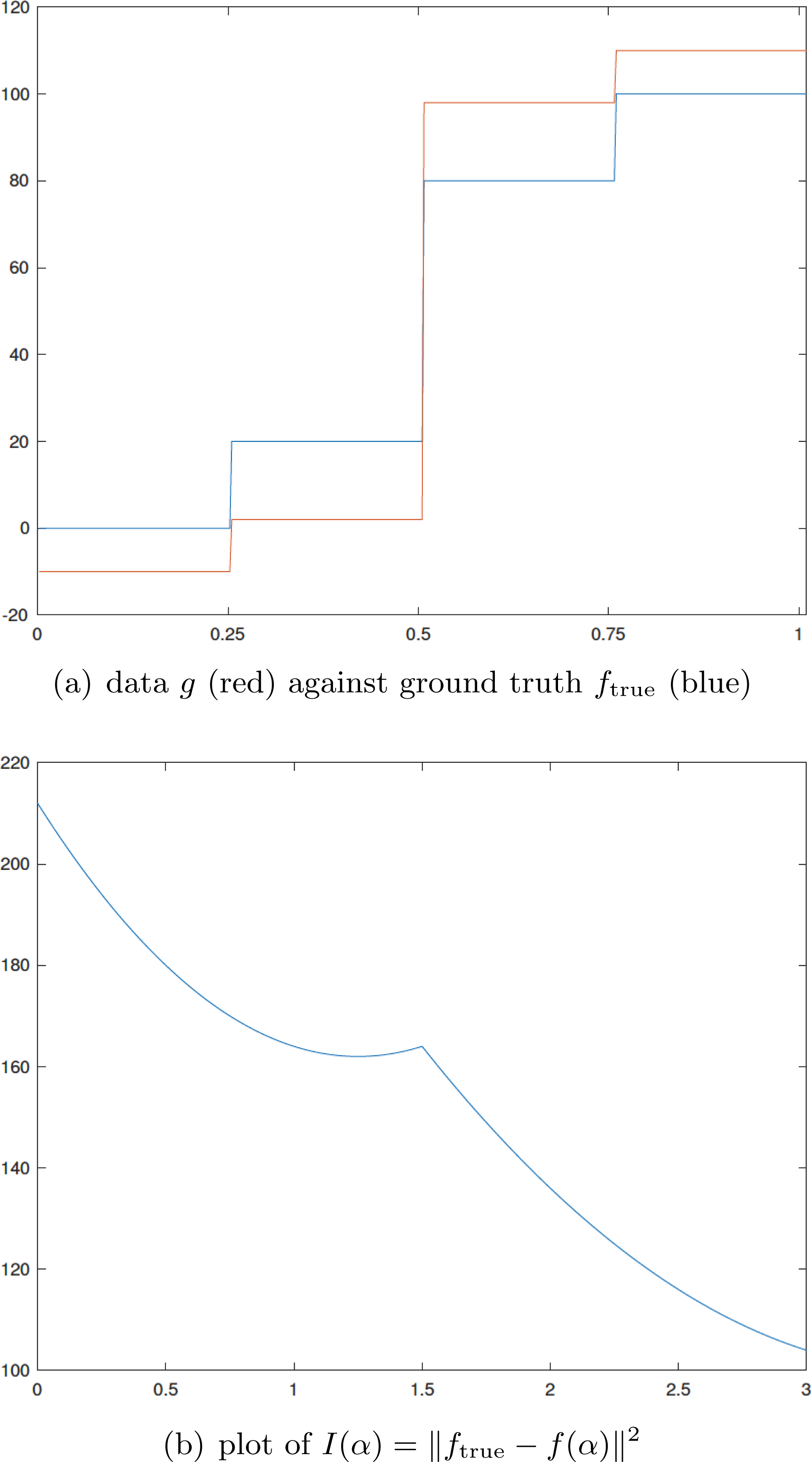
Computing optimal solutions to the bilevel learning problems requires a proper characterization of optimal solutions in terms of a first-order optimality system. Since (4.4)–(4.6) constitutes a PDE-constrained optimization problem, suitable techniques from this field may be utilized. For the limit cases, an additional asymptotic analysis needs to be performed in order to get a sharp characterization of the solutions as
 $\unicode[STIX]{x1D6FE}\rightarrow \infty$
or
$\unicode[STIX]{x1D6FE}\rightarrow \infty$
or
 $\unicode[STIX]{x1D707}\rightarrow 0$
, or both.
$\unicode[STIX]{x1D707}\rightarrow 0$
, or both.
Several instances of the abstract problem (4.4) have been considered in the literature. De los Reyes and Schönlieb (Reference De los Reyes and Schönlieb2013) considered the case with TV regularization in the presence of several noise models. They proved the Gâteaux differentiability of the solution operator, which led to the derivation of an optimality system. Thereafter they carried out an asymptotic analysis with respect to
 $\unicode[STIX]{x1D6FE}\rightarrow \infty$
(with
$\unicode[STIX]{x1D6FE}\rightarrow \infty$
(with
 $\unicode[STIX]{x1D707}>0$
), obtaining an optimality system for the corresponding problem. In that case the optimization problem corresponds to one with variational inequality constraints and the characterization concerns C-stationary points. Also, De los Reyes et al. (Reference De los Reyes, Schönlieb and Valkonen2017) have investigated differentiability properties of higher-order regularization solution operators. They proved a stronger Fréchet-differentiability result for the TGV
$\unicode[STIX]{x1D707}>0$
), obtaining an optimality system for the corresponding problem. In that case the optimization problem corresponds to one with variational inequality constraints and the characterization concerns C-stationary points. Also, De los Reyes et al. (Reference De los Reyes, Schönlieb and Valkonen2017) have investigated differentiability properties of higher-order regularization solution operators. They proved a stronger Fréchet-differentiability result for the TGV
 $^{2}$
case, which also holds for TV. In particular, these stronger results open the door to further necessary and sufficient optimality conditions. Further, using the adjoint optimality condition gradient, formulas for the reduced cost functional can be derived, which in turn feed into the design of numerical algorithms for solving (4.4): see Calatroni et al. (Reference Calatroni, Cao, De los Reyes, Schönlieb and Valkonen2016, Section 3).
$^{2}$
case, which also holds for TV. In particular, these stronger results open the door to further necessary and sufficient optimality conditions. Further, using the adjoint optimality condition gradient, formulas for the reduced cost functional can be derived, which in turn feed into the design of numerical algorithms for solving (4.4): see Calatroni et al. (Reference Calatroni, Cao, De los Reyes, Schönlieb and Valkonen2016, Section 3).
4.3.2 From fields of experts to variational networks
The TV-type regularization approaches discussed above used popular hand-crafted variational regularizers in a first attempt to make them more data-driven, staying in the framework of optimizing proposed regularization models in infinite-dimensional function space. In what follows, we change our perspective to discrete variational regularization models (4.2) in which
 $X=\mathbb{R}^{n}$
, and the functional
$X=\mathbb{R}^{n}$
, and the functional
 ${\mathcal{S}}(\cdot )$
is equipped with parametrizations that go beyond TV-type regularizers; however, these are not covered by the theory in the previous section.
${\mathcal{S}}(\cdot )$
is equipped with parametrizations that go beyond TV-type regularizers; however, these are not covered by the theory in the previous section.
MRF parametrizations.
A prominent example of such richer parametrizations of regularizers has its origins in MRF theory. MRFs, first introduced by Besag (Reference Besag1974) and then used by Cross and Jain (Reference Cross and Jain1983) for texture modelling, provide a probabilistic framework for learning image priors: see e.g. Zhu, Wu and Mumford (Reference Zhu, Wu and Mumford1998). Higher-order MRF models such as the celebrated Field of Experts (FoE) model (Roth and Black Reference Roth and Black2005) are the most popular ones, as they are able to express very complex image structures and yield good performance for various image processing tasks. The FoE model is learning a rich MRF image prior by using ideas from sparse coding (Olshausen and Field Reference Olshausen and Field1997), where image patches are approximated by a linear combination of learned filters, variations of which lead to the well-known principal component analysis (PCA) and independent component analysis (ICA), and the Product of Experts (PoE) model (Welling, Osindero and Hinton Reference Welling, Osindero and Hinton2003).
In the context of bilevel learning, the FoE model has been used by Chen, Pock, Ranftl and Bischof (Reference Chen, Pock, Ranftl and Bischof2013) and Chen, Ranftl and Pock (Reference Chen, Ranftl and Pock2014). Here, the regularizer is parametrized in the form
 $$\begin{eqnarray}{\mathcal{S}}_{\unicode[STIX]{x1D703}}(f) :=\mathop{\sum }_{i=1}^{N}\left[\unicode[STIX]{x1D6FC}_{i}\mathop{\sum }_{k=1}^{n}\unicode[STIX]{x1D70C}((J_{i}f)_{k})\right]\quad \text{with }\unicode[STIX]{x1D703}=(\unicode[STIX]{x1D6FC}_{1},\ldots ,\unicode[STIX]{x1D6FC}_{N},J_{1},\ldots ,J_{N}),\end{eqnarray}$$
where
 $N$
is the number of filters
$N$
is the number of filters
 $J_{i}$
which are sparse and implemented as a two-dimensional convolution with a kernel
$J_{i}$
which are sparse and implemented as a two-dimensional convolution with a kernel
 $k_{i}$
, that is,
$k_{i}$
, that is,
 $J_{i}f$
is the digitized version of
$J_{i}f$
is the digitized version of
 $k_{i}\ast f$
. In the FoE model we use the parametrization
$k_{i}\ast f$
. In the FoE model we use the parametrization
 $J_{i}=\sum _{j=1}^{m}\unicode[STIX]{x1D6FD}_{i,j}B_{j}$
, for a given set of basis filters
$J_{i}=\sum _{j=1}^{m}\unicode[STIX]{x1D6FD}_{i,j}B_{j}$
, for a given set of basis filters
 $\{B_{1},\ldots ,B_{m}\}$
with
$\{B_{1},\ldots ,B_{m}\}$
with
 $B_{j}\in \mathbb{R}^{n\times n}$
. Moreover, the
$B_{j}\in \mathbb{R}^{n\times n}$
. Moreover, the
 $\unicode[STIX]{x1D6FC}_{i}$
are non-negative parameters and the non-linear function
$\unicode[STIX]{x1D6FC}_{i}$
are non-negative parameters and the non-linear function
 $\unicode[STIX]{x1D70C}(z)=\log (1+z^{2})$
. The shape of
$\unicode[STIX]{x1D70C}(z)=\log (1+z^{2})$
. The shape of
 $\unicode[STIX]{x1D70C}$
is motivated by statistics over natural images that were shown to roughly follow a Student
$\unicode[STIX]{x1D70C}$
is motivated by statistics over natural images that were shown to roughly follow a Student
 $t$
-distribution (Huang and Mumford Reference Huang and Mumford1999). With these parametrizations,
$t$
-distribution (Huang and Mumford Reference Huang and Mumford1999). With these parametrizations,
 $\unicode[STIX]{x1D703}$
in (4.7) can be seen as
$\unicode[STIX]{x1D703}$
in (4.7) can be seen as
 $\unicode[STIX]{x1D703}=(\unicode[STIX]{x1D6FC}_{i},\unicode[STIX]{x1D6FD}_{i,j})$
for
$\unicode[STIX]{x1D703}=(\unicode[STIX]{x1D6FC}_{i},\unicode[STIX]{x1D6FD}_{i,j})$
for
 $i=1,\ldots ,n$
and
$i=1,\ldots ,n$
and
 $j=1,\ldots ,m$
, and one learns the optimal
$j=1,\ldots ,m$
, and one learns the optimal
 $\unicode[STIX]{x1D703}$
from supervised training data
$\unicode[STIX]{x1D703}$
from supervised training data
 $(f_{i},g_{i})$
by minimizing the squared
$(f_{i},g_{i})$
by minimizing the squared
 $L^{2}$
-loss:
$L^{2}$
-loss:
 $$\begin{eqnarray}\ell _{X}({\mathcal{R}}_{\unicode[STIX]{x1D703}}(g),f) :=\Vert {\mathcal{R}}_{\unicode[STIX]{x1D703}}(g)-f\Vert _{2}^{2}\quad \text{with }{\mathcal{R}}_{\unicode[STIX]{x1D703}}:Y\rightarrow X\text{ given by (4.4)}.\end{eqnarray}$$
Chen et al. (Reference Chen, Ranftl and Pock2014) investigated other non-linearities such as the non-smooth and non-convex
 $\unicode[STIX]{x1D70C}(z)=\log (1+|z|)$
, and the non-smooth but convex
$\unicode[STIX]{x1D70C}(z)=\log (1+|z|)$
, and the non-smooth but convex
 $\ell _{1}$
-norm
$\ell _{1}$
-norm
 $\unicode[STIX]{x1D70C}(z)=|z|$
. Their experiments in particular suggested that, while the two
$\unicode[STIX]{x1D70C}(z)=|z|$
. Their experiments in particular suggested that, while the two
 $\log$
-type non-linearities gave very similar regularization performance, the convex
$\log$
-type non-linearities gave very similar regularization performance, the convex
 $\ell _{1}$
-norm regularizer clearly did worse. Moreover, Chen et al. (Reference Chen, Yu and Pock2015) parametrized the non-linearities
$\ell _{1}$
-norm regularizer clearly did worse. Moreover, Chen et al. (Reference Chen, Yu and Pock2015) parametrized the non-linearities
 $\unicode[STIX]{x1D70C}$
with radial basis functions, whose coefficients are learned as well. Earlier MRF-based bilevel learning schemes exist: see e.g. Samuel and Tappen (Reference Samuel and Tappen2009).
$\unicode[STIX]{x1D70C}$
with radial basis functions, whose coefficients are learned as well. Earlier MRF-based bilevel learning schemes exist: see e.g. Samuel and Tappen (Reference Samuel and Tappen2009).
A further development is the variational networks introduced by Kobler, Klatzer, Hammernik and Pock (Reference Kobler, Klatzer, Hammernik and Pock2017) and Hammernik et al. (Reference Hammernik, Klatzer, Kobler, Recht, Sodickson, Pock and Knoll2018). The idea was to replace the above bilevel scheme with learning to optimize (Section 4.9) using a supervised loss, thereby leading to a learned iterative method. This will be discussed in more detail in Section 5.1.4, where the variational networks re-emerge in the framework of learned iterative schemes.
4.4 Dictionary learning in sparse models
In Section 2.7 we discussed sparsity as an important concept for modelling prior knowledge in inverse problems. Assuming that the model parameter possesses a sparse or compressible representation in a given dictionary
 $\mathbb{D}$
sparse recovery strategies, associated computational approaches and error estimates for the model parameter can be derived. In what follows, we turn to approaches which, rather than working with a given dictionary, learn the dictionary before or jointly with the recovery of the model parameter. Note that almost all work on dictionary learning in sparse models has been carried out in the context of denoising, i.e.
$\mathbb{D}$
sparse recovery strategies, associated computational approaches and error estimates for the model parameter can be derived. In what follows, we turn to approaches which, rather than working with a given dictionary, learn the dictionary before or jointly with the recovery of the model parameter. Note that almost all work on dictionary learning in sparse models has been carried out in the context of denoising, i.e.
 ${\mathcal{A}}=\text{id}$
only.
${\mathcal{A}}=\text{id}$
only.
Patch-based local models.
A particular class of sparse coding models are those which impose sparsity on patches (segmented) that are extracted from the signal. Let
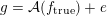 $g={\mathcal{A}}(f_{\text{true}})+e$
and
$g={\mathcal{A}}(f_{\text{true}})+e$
and
 $\hat{f}\in X$
. Further, let
$\hat{f}\in X$
. Further, let
 $\mathbb{D}=\{\unicode[STIX]{x1D719}_{k}\}\subset X$
be a dictionary, and
$\mathbb{D}=\{\unicode[STIX]{x1D719}_{k}\}\subset X$
be a dictionary, and
 $P_{j}:X\rightarrow X$
with
$P_{j}:X\rightarrow X$
with
 $P_{j}(f)=f|_{\unicode[STIX]{x1D6FA}_{j}}$
for
$P_{j}(f)=f|_{\unicode[STIX]{x1D6FA}_{j}}$
for
 $j=1,\ldots N$
patches of
$j=1,\ldots N$
patches of
 $f$
. Assume that
$f$
. Assume that
 $$\begin{eqnarray}\hat{f}=\mathop{\sum }_{j=1}^{N}P_{j}(f_{\text{true}}),\end{eqnarray}$$
where
 $P_{j}(f_{\text{true}})\in X$
is compressible with respect to
$P_{j}(f_{\text{true}})\in X$
is compressible with respect to
 $\mathbb{D}$
.
$\mathbb{D}$
.
Some of the currently leading denoising methods are based on patch-based local models. Examples include K-SVD, which is a sparse coding approach on image patches (Elad and Aharon Reference Elad and Aharon2006), BM3D, which combines sparsity and self-similarity (Dabov, Foi, Katkovnik and Egiazarian Reference Dabov, Foi, Katkovnik and Egiazarian2007), and EPLL, which is a Gaussian mixture model of image patches (Zoran and Weiss Reference Zoran and Weiss2011). Other examples are NCSR (Dong, Zhang, Shi and Li Reference Dong, Zhang, Shi and Li2013), weighted nuclear norm regularization of image patches (WNNM) (Gu, Zhang, Zuo and Feng Reference Gu, Zhang, Zuo and Feng2014) and SSC-GSM, a non-local sparsity approach with a Gaussian scale mixture (Dong, Shi, Ma and Li Reference Dong, Shi, Ma and Li2015).
Sparse-land models are a particular subclass of patch-based models. Here, each patch is sparse with respect to some global dictionary. Examples include sparse coding approaches that are applied patch-wise (Elad and Aharon Reference Elad and Aharon2006, Dong, Zhang, Shi and Wu Reference Dong, Zhang, Shi and Wu2011, Mairal and Ponce Reference Mairal and Ponce2014, Romano and Elad Reference Romano and Elad2015, Sulam and Elad Reference Sulam and Elad2015). In sparse-land models
 $\hat{f}\in X$
is reconstructed by solving
$\hat{f}\in X$
is reconstructed by solving
 $$\begin{eqnarray}\min _{f\in X,\unicode[STIX]{x1D709}_{i}\in \unicode[STIX]{x1D6EF}}\{{\mathcal{L}}({\mathcal{A}}(f),g)+{\mathcal{S}}_{\unicode[STIX]{x1D703}}(f,\unicode[STIX]{x1D709}_{1},\ldots ,\unicode[STIX]{x1D709}_{N})\},\end{eqnarray}$$
where
 $$\begin{eqnarray}{\mathcal{S}}_{\unicode[STIX]{x1D703}}(f,\unicode[STIX]{x1D709}_{1},\ldots ,\unicode[STIX]{x1D709}_{N}) :=\mathop{\sum }_{j=1}^{N}[\unicode[STIX]{x1D706}_{j}\Vert P_{j}(f)-{\mathcal{E}}_{\mathbb{D}}^{\ast }(\unicode[STIX]{x1D709}_{j})\Vert _{2}^{2}+\unicode[STIX]{x1D707}_{j}\Vert \unicode[STIX]{x1D709}_{j}\Vert _{p}^{p}],\end{eqnarray}$$
with
 $\unicode[STIX]{x1D703}=(\unicode[STIX]{x1D706}_{j},\unicode[STIX]{x1D707}_{j})_{j=1}^{N}\in (\mathbb{R}^{2})^{N}$
and
$\unicode[STIX]{x1D703}=(\unicode[STIX]{x1D706}_{j},\unicode[STIX]{x1D707}_{j})_{j=1}^{N}\in (\mathbb{R}^{2})^{N}$
and
 ${\mathcal{E}}_{\mathbb{D}}^{\ast }:\unicode[STIX]{x1D6EF}\rightarrow X$
denoting the synthesis operator associated with the given dictionary
${\mathcal{E}}_{\mathbb{D}}^{\ast }:\unicode[STIX]{x1D6EF}\rightarrow X$
denoting the synthesis operator associated with the given dictionary
 $\mathbb{D}$
. Bai et al. (Reference Bai, Yan, Jia, Jiang, Wang and Mou2017) propose the following alternating scheme to solve the sparse-land reconstruction problem:
$\mathbb{D}$
. Bai et al. (Reference Bai, Yan, Jia, Jiang, Wang and Mou2017) propose the following alternating scheme to solve the sparse-land reconstruction problem:
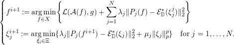
The advantage of these approaches over plain-vanilla dictionary learning is that sparse-land models are computationally more feasible. Sparse-land models are one example of a dictionary learning approach, which will be discussed in the next section.
4.4.1 Reconstruction and dictionary learning
In sparse models, there are three ways to determine the dictionary. First, the dictionary is specified analytically. Second, the dictionary is determined from example data (dictionary learning). Third (as in the sparse-land models discussed above) the dictionary is determined jointly while performing reconstruction (joint reconstruction and dictionary learning). In what follows, we particularly focus on the second and third options for determining the dictionary.
Joint reconstruction and dictionary learning.
The recent paper by Chambolle, Holler and Pock (Reference Chambolle, Holler and Pock2018) proposes a convex variational model for joint reconstruction and (convolutional) dictionary learning that applies to inverse problems where data are corrupted and/or incomplete. Chambolle et al. (Reference Chambolle, Holler and Pock2018) prove rigorous results on well-posedness and stability stated in the infinite-dimensional (non-digitized) setting.
Earlier approaches were less rigorous and considered the finite-dimensional setting with a patch-based dictionary (sparse-land model). One such example is adaptive dictionary-based statistical iterative reconstruction (ADSIR) (Zhang et al.
Reference Zhang, Zhang, Li, Peng, Liu and Zheng2016), which adds the dictionary
 $\mathbb{D}=\{\unicode[STIX]{x1D719}_{i}\}\subset X$
as an unknown to the sparse-land model as in global dictionary-based statistical iterative reconstruction (GDSIR) (Xu et al. Reference Xu, Yu, Mou, Zhang, Hsieh and Wang2012; see also Chun, Zheng, Long and Fessler Reference Chun, Zheng, Long and Fessler2017). This results in the following problem:
$\mathbb{D}=\{\unicode[STIX]{x1D719}_{i}\}\subset X$
as an unknown to the sparse-land model as in global dictionary-based statistical iterative reconstruction (GDSIR) (Xu et al. Reference Xu, Yu, Mou, Zhang, Hsieh and Wang2012; see also Chun, Zheng, Long and Fessler Reference Chun, Zheng, Long and Fessler2017). This results in the following problem:
 $$\begin{eqnarray}\min _{f\in X,\unicode[STIX]{x1D709}_{i}\in \unicode[STIX]{x1D6EF},\mathbb{D}}\{{\mathcal{L}}({\mathcal{A}}(f),g)+{\mathcal{S}}_{\unicode[STIX]{x1D703}}(f,\unicode[STIX]{x1D709}_{1},\ldots ,\unicode[STIX]{x1D709}_{N},\mathbb{D})\},\end{eqnarray}$$
where
 $$\begin{eqnarray}{\mathcal{S}}_{\unicode[STIX]{x1D703}}(f,\unicode[STIX]{x1D709}_{1},\ldots ,\unicode[STIX]{x1D709}_{N},\mathbb{D}):=\mathop{\sum }_{j=1}^{N}[\unicode[STIX]{x1D706}_{j}\Vert P_{j}(f)-{\mathcal{E}}_{\mathbb{D}}^{\ast }(\unicode[STIX]{x1D709}_{j})\Vert _{2}^{2}+\unicode[STIX]{x1D707}_{j}\Vert \unicode[STIX]{x1D709}_{j}\Vert _{p}^{p}],\end{eqnarray}$$
with
 $\unicode[STIX]{x1D703}=((\unicode[STIX]{x1D706}_{j},\unicode[STIX]{x1D707}_{j})_{j=1}^{N})\in (\mathbb{R}^{2})^{N}$
, and
$\unicode[STIX]{x1D703}=((\unicode[STIX]{x1D706}_{j},\unicode[STIX]{x1D707}_{j})_{j=1}^{N})\in (\mathbb{R}^{2})^{N}$
, and
 ${\mathcal{E}}_{\mathbb{D}}^{\ast }:\unicode[STIX]{x1D6EF}\rightarrow X$
denotes the synthesis operator associated with the dictionary
${\mathcal{E}}_{\mathbb{D}}^{\ast }:\unicode[STIX]{x1D6EF}\rightarrow X$
denotes the synthesis operator associated with the dictionary
 $\mathbb{D}$
. Usually an alternating minimization scheme is used to optimize over the three variables in (4.12).
$\mathbb{D}$
. Usually an alternating minimization scheme is used to optimize over the three variables in (4.12).
Dictionary learning.
Let
 $\ell _{X}:X\times X\rightarrow \mathbb{R}$
be a given loss function (e.g. the
$\ell _{X}:X\times X\rightarrow \mathbb{R}$
be a given loss function (e.g. the
 $\ell _{2}$
- or
$\ell _{2}$
- or
 $\ell _{1}$
-norm). Further, let
$\ell _{1}$
-norm). Further, let
 $f_{1}\ldots f_{N}\in X$
be a given unsupervised training data,
$f_{1}\ldots f_{N}\in X$
be a given unsupervised training data,
 $\mathbb{D}=\{\unicode[STIX]{x1D719}_{i}\}\subset X$
a dictionary, and
$\mathbb{D}=\{\unicode[STIX]{x1D719}_{i}\}\subset X$
a dictionary, and
 ${\mathcal{E}}_{\mathbb{D}}^{\ast }:\unicode[STIX]{x1D6EF}\rightarrow X$
the synthesis operator given as
${\mathcal{E}}_{\mathbb{D}}^{\ast }:\unicode[STIX]{x1D6EF}\rightarrow X$
the synthesis operator given as
 ${\mathcal{E}}_{\mathbb{D}}^{\ast }(\unicode[STIX]{x1D709})=\sum _{i}\unicode[STIX]{x1D709}_{i}\unicode[STIX]{x1D719}_{i}$
for
${\mathcal{E}}_{\mathbb{D}}^{\ast }(\unicode[STIX]{x1D709})=\sum _{i}\unicode[STIX]{x1D709}_{i}\unicode[STIX]{x1D719}_{i}$
for
 $\unicode[STIX]{x1D709}\in \unicode[STIX]{x1D6EF}$
. One approach in dictionary learning is based on a sparsity assumption and solves
$\unicode[STIX]{x1D709}\in \unicode[STIX]{x1D6EF}$
. One approach in dictionary learning is based on a sparsity assumption and solves
such that
 $\Vert \unicode[STIX]{x1D709}_{i}\Vert _{0}\leq s$
for
$\Vert \unicode[STIX]{x1D709}_{i}\Vert _{0}\leq s$
for
 $i=1,\ldots ,N$
, for a given sparsity level
$i=1,\ldots ,N$
, for a given sparsity level
 $s$
. Alternatively, one looks for a dictionary that minimizes the total cost for representing signals in the training data while enforcing a constraint on the precision in the following way:
$s$
. Alternatively, one looks for a dictionary that minimizes the total cost for representing signals in the training data while enforcing a constraint on the precision in the following way:
such that
 $\ell _{X}(f_{i},{\mathcal{E}}_{\mathbb{D}}^{\ast }(\unicode[STIX]{x1D709}_{i}))\leq \unicode[STIX]{x1D716}$
for
$\ell _{X}(f_{i},{\mathcal{E}}_{\mathbb{D}}^{\ast }(\unicode[STIX]{x1D709}_{i}))\leq \unicode[STIX]{x1D716}$
for
 $i=1,\ldots ,N$
. A unified formulation is given by the unconstrained problem
$i=1,\ldots ,N$
. A unified formulation is given by the unconstrained problem
All three formulations are posed in terms of the
 $\ell _{0}$
-norm and are NP-hard to compute. This suggests the use of convex relaxation, by which (4.16) becomes
$\ell _{0}$
-norm and are NP-hard to compute. This suggests the use of convex relaxation, by which (4.16) becomes
If
 $\mathbb{D}$
is fixed then the sum in (4.17) decouples and leads to the convex relaxation of the sparse coding problem in (2.20) for
$\mathbb{D}$
is fixed then the sum in (4.17) decouples and leads to the convex relaxation of the sparse coding problem in (2.20) for
 ${\mathcal{A}}=\text{id}$
.
${\mathcal{A}}=\text{id}$
.
In the finite-dimensional setting
 $X=\mathbb{R}^{m}$
and
$X=\mathbb{R}^{m}$
and
 $\unicode[STIX]{x1D6EF}$
is replaced by
$\unicode[STIX]{x1D6EF}$
is replaced by
 $\mathbb{R}^{n}$
for some
$\mathbb{R}^{n}$
for some
 $n$
. Then the dictionary is
$n$
. Then the dictionary is
 $\mathbb{D}:=\{{\unicode[STIX]{x1D719}_{k}\}}_{k=1\ldots n}\subset \mathbb{R}^{m}$
represented by an
$\mathbb{D}:=\{{\unicode[STIX]{x1D719}_{k}\}}_{k=1\ldots n}\subset \mathbb{R}^{m}$
represented by an
 $n\times m$
matrix
$n\times m$
matrix
 $\mathbf{\mathsf{D}}$
leading to the synthesis operator becoming a mapping
$\mathbf{\mathsf{D}}$
leading to the synthesis operator becoming a mapping
 ${\mathcal{E}}_{\mathbf{\mathsf{D}}}^{\ast }:\mathbb{R}^{m}\rightarrow \mathbb{R}^{n}$
with
${\mathcal{E}}_{\mathbf{\mathsf{D}}}^{\ast }:\mathbb{R}^{m}\rightarrow \mathbb{R}^{n}$
with
 ${\mathcal{E}}_{\mathbb{D}}^{\ast }(\unicode[STIX]{x1D709})=\mathbf{\mathsf{D}}\cdot \unicode[STIX]{x1D709}$
. In this setting (4.17) becomes
${\mathcal{E}}_{\mathbb{D}}^{\ast }(\unicode[STIX]{x1D709})=\mathbf{\mathsf{D}}\cdot \unicode[STIX]{x1D709}$
. In this setting (4.17) becomes
Here, if
 $\mathbf{\mathsf{D}}$
satisfies the RIP then the convex relaxation preserves the sparse solution (Candès et al.
Reference Candès, Romberg and Tao2006). State-of-the-art dictionary learning algorithms are K-SVD (Aharon, Elad and Bruckstein Reference Aharon, Elad and Bruckstein2006), geometric multi-resolution analysis (GRMA) (Allard, Chen and Maggioni Reference Allard, Chen and Maggioni2012) and online dictionary learning (Mairal, Bach, Ponce and Sapiro Reference Mairal, Bach, Ponce and Sapiro2010). Most work on dictionary learning to date has been done in the context of denoising, i.e.
$\mathbf{\mathsf{D}}$
satisfies the RIP then the convex relaxation preserves the sparse solution (Candès et al.
Reference Candès, Romberg and Tao2006). State-of-the-art dictionary learning algorithms are K-SVD (Aharon, Elad and Bruckstein Reference Aharon, Elad and Bruckstein2006), geometric multi-resolution analysis (GRMA) (Allard, Chen and Maggioni Reference Allard, Chen and Maggioni2012) and online dictionary learning (Mairal, Bach, Ponce and Sapiro Reference Mairal, Bach, Ponce and Sapiro2010). Most work on dictionary learning to date has been done in the context of denoising, i.e.
 ${\mathcal{A}}=\text{id}$
; see also Rubinstein et al. (Reference Rubinstein, Bruckstein and Elad.2010).
${\mathcal{A}}=\text{id}$
; see also Rubinstein et al. (Reference Rubinstein, Bruckstein and Elad.2010).
4.4.2 Convolutional sparse coding and convolutional dictionary learning
Dictionary learning in the context of sparse coding has been very popular and successful, with several seminal approaches arising in this field, as outlined in the previous section. However, there are still several issues with sparse coding related to the locality of learned structures and the computational effort needed. Sparse-land models (4.9), for instance, perform sparse coding over all the patches, and this tends to be a slow process.
The computational performance can be addressed by using learning to improve upon an optimization scheme (Section 4.9), for example the Learned Iterative Soft-Thresholding Algorithm (LISTA) (see Section 4.9.2) learns a finite number of unrolled Iterative Soft-Thresholding Algorithm (ISTA) iterates using unsupervised training data to match ISTA solutions (Gregor and LeCun Reference Gregor and LeCun2010). Moreover, learning a dictionary over each patch independently as in (4.12) cannot account for global information, e.g. shift-invariance in images. What is needed is a computational feasible approach that introduces further structure and invariances in the dictionary, e.g. shift-invariance, and that makes each atom dependent on the whole signal instead of just individual patches. In this realm convolutional dictionaries have been introduced. Here atoms are given by convolution kernels and act on signal features via convolution, that is,
 $\mathbf{\mathsf{D}}$
is a concatenation of Toeplitz matrices (a union of banded and circulant matrices). Set up like this, convolutional dictionaries render computationally feasible shift-invariant dictionaries, where atoms depend on the entire signal.
$\mathbf{\mathsf{D}}$
is a concatenation of Toeplitz matrices (a union of banded and circulant matrices). Set up like this, convolutional dictionaries render computationally feasible shift-invariant dictionaries, where atoms depend on the entire signal.
Convolutional sparse coding.
Consider now the inverse problem of recovering
 $f_{\text{true}}\in X$
from (2.1) with the assumption that
$f_{\text{true}}\in X$
from (2.1) with the assumption that
 $f_{\text{true}}$
is compressible with respect to convolution dictionary
$f_{\text{true}}$
is compressible with respect to convolution dictionary
 $\mathbb{D}:=\{\unicode[STIX]{x1D719}_{i}\}\subset X$
.
$\mathbb{D}:=\{\unicode[STIX]{x1D719}_{i}\}\subset X$
.
In convolutional sparse coding (CSC), this is done by performing a synthesis using convolutional dictionaries, that is, atoms act by convolutions. More precisely, the reconstruction operator
 ${\mathcal{R}}_{\unicode[STIX]{x1D703}}:Y\rightarrow X$
is given as
${\mathcal{R}}_{\unicode[STIX]{x1D703}}:Y\rightarrow X$
is given as
 $$\begin{eqnarray}{\mathcal{R}}(g):=\mathop{\sum }_{i}\hat{\unicode[STIX]{x1D709}}_{i}\ast \unicode[STIX]{x1D719}_{i},\end{eqnarray}$$
where
Computational methods for solving (4.19) for denoising use convex relaxation followed by the alternating direction method of multipliers (ADMM) in frequency space (Bristow, Eriksson and Lucey Reference Bristow, Eriksson and Lucey2013) and its variants. See also Sreter and Giryes (Reference Sreter and Giryes2017) on using Learned Iterative Soft-Thresholding Algorithm (LISTA) in this context. So far CSC has only been analysed in the context of denoising (Bristow et al. Reference Bristow, Eriksson and Lucey2013, Wohlberg Reference Wohlberg2014, Gu et al. Reference Gu, Zuo, Xie, Meng, Feng and Zhang2015, Garcia-Cardona and Wohlberg Reference Garcia-Cardona and Wohlberg2017) with theoretical properties given in Papyan, Sulam and Elad (Reference Papyan, Sulam and Elad2016a , Reference Papyan, Sulam and Elad2016b ).
Convolutional dictionary learning.
Learning a dictionary in the context of CSC is called convolutional dictionary learning. Here, given unsupervised training data
 $f_{1},\ldots ,f_{m}\in X$
and a loss function
$f_{1},\ldots ,f_{m}\in X$
and a loss function
 $\ell _{X}:X:X\rightarrow X$
, one solves
$\ell _{X}:X:X\rightarrow X$
, one solves
where
 $\Vert \unicode[STIX]{x1D719}_{i}\Vert _{2}=1$
. For instance, Garcia-Cardona and Wohlberg (Reference Garcia-Cardona and Wohlberg2017) solved (4.20) with a squared
$\Vert \unicode[STIX]{x1D719}_{i}\Vert _{2}=1$
. For instance, Garcia-Cardona and Wohlberg (Reference Garcia-Cardona and Wohlberg2017) solved (4.20) with a squared
 $L_{2}$
-loss using an ADMM-type scheme. Extension of convolutional dictionary learning to a supervised data setting has been considered by Affara, Ghanem and Wonka (Reference Affara, Ghanem and Wonka2018), for instance. Here, discriminative dictionaries instead of purely reconstructive ones are learned by introducing a supervised regularization term in the usual CSC objective that encourages the final dictionary elements to be discriminative.
$L_{2}$
-loss using an ADMM-type scheme. Extension of convolutional dictionary learning to a supervised data setting has been considered by Affara, Ghanem and Wonka (Reference Affara, Ghanem and Wonka2018), for instance. Here, discriminative dictionaries instead of purely reconstructive ones are learned by introducing a supervised regularization term in the usual CSC objective that encourages the final dictionary elements to be discriminative.
Multi-layer convolutional sparse coding.
A multi-layer extension of CSC, referred to as multi-layer convolutional sparse coding (ML-CSC), is proposed by Sulam, Papyan, Romano and Elad (Reference Sulam, Papyan, Romano and Elad2017). Given
 $L$
convolutional dictionaries
$L$
convolutional dictionaries
 $\mathbb{D}_{1},\ldots ,\mathbb{D}_{L}\subset X$
with atoms
$\mathbb{D}_{1},\ldots ,\mathbb{D}_{L}\subset X$
with atoms
 $\mathbb{D}_{k}:=\{\unicode[STIX]{x1D719}_{j}^{k}\}_{j}$
, a model parameter
$\mathbb{D}_{k}:=\{\unicode[STIX]{x1D719}_{j}^{k}\}_{j}$
, a model parameter
 $f\in X$
admits a representation in terms of the corresponding multi-layer convolutional sparse coding (ML-CSC) model if there are
$f\in X$
admits a representation in terms of the corresponding multi-layer convolutional sparse coding (ML-CSC) model if there are
 $s_{1},\ldots ,s_{L}\in \mathbb{R}$
such that
$s_{1},\ldots ,s_{L}\in \mathbb{R}$
such that
 $$\begin{eqnarray}\left\{\begin{array}{@{}ll@{}}f=\mathop{\sum }_{j}(\unicode[STIX]{x1D709}_{j}^{1}\ast \unicode[STIX]{x1D719}_{j}^{1}),\quad & \\[4.0pt] \boldsymbol{\unicode[STIX]{x1D709}}^{k}=\mathop{\sum }_{j}(\unicode[STIX]{x1D709}_{j}^{k+1}\ast \unicode[STIX]{x1D719}_{j}^{k+1})\quad \text{for }k=1,\ldots ,L-1,\quad & \end{array}\right.\end{eqnarray}$$
and
 $\Vert \boldsymbol{\unicode[STIX]{x1D709}}^{k}\Vert _{0,\infty }\leq s_{k}$
for
$\Vert \boldsymbol{\unicode[STIX]{x1D709}}^{k}\Vert _{0,\infty }\leq s_{k}$
for
 $k=1,\ldots ,L$
. Hence, atoms
$k=1,\ldots ,L$
. Hence, atoms
 $\unicode[STIX]{x1D719}_{k,i}\in \mathbb{D}_{k}$
in the
$\unicode[STIX]{x1D719}_{k,i}\in \mathbb{D}_{k}$
in the
 $k$
th convolution dictionary are compressible in the
$k$
th convolution dictionary are compressible in the
 $(k+1)$
th dictionary
$(k+1)$
th dictionary
 $\mathbb{D}_{k+1}$
for
$\mathbb{D}_{k+1}$
for
 $k=1,\ldots ,L-1$
.
$k=1,\ldots ,L-1$
.
The ML-CSC model is a special case of CSC where intermediate representations have a specific structure (Sulam et al. Reference Sulam, Papyan, Romano and Elad2017, Lemma 1). Building on the theory for CSC, Sulam et al. (Reference Sulam, Papyan, Romano and Elad2017) provide a theoretical study of this novel model and its associated pursuits for dictionary learning and sparse coding in the context of denoising. Further, consequences for the theoretical analysis of partial differential equations (CNNs) can be extracted from ML-CSC using the fact that the resulting layered thresholding algorithm and the layered basis pursuit share many similarities with a forward pass of a deep CNN.
Indeed, Papyan, Romano and Elad (Reference Papyan, Romano and Elad2017) show that ML-CSC yields a Bayesian model that is implicitly imposed on
 $\hat{f}$
when deploying a CNN, and that consequently characterizes signals belonging to the model behind a deep CNN. Among other properties, one can show that the CNN is guaranteed to recover an estimate of the underlying representations of an input signal, assuming these are sparse in a local sense (Papyan et al.
Reference Papyan, Romano and Elad2017, Theorem 4) and the recovery is stable (Papyan et al.
Reference Papyan, Romano and Elad2017, Theorems 8 and 10). Many of these results also hold for fully connected networks, and they can be used to formulate new algorithms for partial differential equations (CNNs), for example to propose an alternative to the commonly used forward pass algorithm in CNN. This is related to both deconvolutional (Zeiler, Krishnan, Taylor and Fergus Reference Zeiler, Krishnan, Taylor and Fergus2010, Pu et al.
Reference Pu, Yuan, Stevens, Li and Carin2016) and recurrent networks (Bengio, Simard and Frasconi Reference Bengio, Simard and Frasconi1994).
$\hat{f}$
when deploying a CNN, and that consequently characterizes signals belonging to the model behind a deep CNN. Among other properties, one can show that the CNN is guaranteed to recover an estimate of the underlying representations of an input signal, assuming these are sparse in a local sense (Papyan et al.
Reference Papyan, Romano and Elad2017, Theorem 4) and the recovery is stable (Papyan et al.
Reference Papyan, Romano and Elad2017, Theorems 8 and 10). Many of these results also hold for fully connected networks, and they can be used to formulate new algorithms for partial differential equations (CNNs), for example to propose an alternative to the commonly used forward pass algorithm in CNN. This is related to both deconvolutional (Zeiler, Krishnan, Taylor and Fergus Reference Zeiler, Krishnan, Taylor and Fergus2010, Pu et al.
Reference Pu, Yuan, Stevens, Li and Carin2016) and recurrent networks (Bengio, Simard and Frasconi Reference Bengio, Simard and Frasconi1994).
An essential technique for proving the key results in the cited references for ML-CSC is based on unrolling, which establishes a link between sparsity-promoting regularization (compressed sensing) and deep neural networks. More precisely, one starts with a variational formulation like that in (4.20) and specifies a suitable iterative optimization scheme. In this setting one can prove several theoretical results, such as convergence, stability and error estimates. Next, one unrolls the truncated optimization iterates and identifies the updating between iterates as layers in a deep neural network (Section 4.9.1). The properties of this network, such as stability and convergence, can now be analysed using methods from compressed sensing.
Deep dictionary learning.
Another recent approach in the context of dictionary learning is deep dictionary learning. Here, the two popular representation learning paradigms – dictionary learning and deep learning – come together. Conceptually, while dictionary learning focuses on learning a ‘basis’ and ‘features’ by matrix factorization, deep learning focuses on extracting features via learning ‘weights’ or ‘filters’ in a greedy layer-by-layer fashion. Deep dictionary learning, in turn, builds deeper architectures by using the layers of dictionary learning. See Tariyal, Majumdar, Singh and Vatsa (Reference Tariyal, Majumdar, Singh and Vatsa2016), who show that their approach is competitive against other deep learning approaches, such as stacked auto-encoders, deep belief networks and convolutional neural networks, regarding classification and clustering accuracies.
4.4.3 TV-type regularizer with learned sparsifying transforms.
The idea here is to learn the underlying sparsifying transform in a TV-type regularizer. One such approach is presented by Chun, Zheng, Long and Fessler (Reference Chun, Zheng, Long and Fessler2017), who consider the case of a single sparsifying transform. This idea is further developed by Zheng, Ravishankar, Long and Fessler (Reference Zheng, Ravishankar, Long and Fessler2018), who consider a regularizer that is given by a union of sparsifying transforms (ULTRA), which act on image patches and quantify the sparsification error of each patch using its best-matched sparsifying transform: see Zheng et al. (Reference Zheng, Ravishankar, Long and Fessler2018, equation (3)). The resulting optimization problem is solved by an intertwined scheme that alternates between a CT image reconstruction step, calculated via a relaxed linearized augmented Lagrangian method with ordered subsets, and a sparse coding and clustering step, which simultaneously groups the training patches into a fixed number of clusters and learns a transform in each cluster along with the sparse coefficients (in the transform domain) of the patches.
A variant of Zheng et al. (Reference Zheng, Ravishankar, Long and Fessler2018) is considered by Ye, Ravishankar, Long and Fessler (Reference Ye, Ravishankar, Long and Fessler2018b ), who use the same pre-learned union of sparsifying transforms as in Zheng et al. (Reference Zheng, Ravishankar, Long and Fessler2018), but the alternating scheme also includes iteratively updating a quadratic surrogate functions for the data discrepancy. These variants of learned sparsifying transforms are all applied to low-dose CT image reconstruction. Finally, Chen et al. (Reference Chen, Xiang, Gong, Wang and Tan2018) use essentially the method of Zheng et al. (Reference Zheng, Ravishankar, Long and Fessler2018) applied to cone-beam CT.
4.5 Scattering networks
Scattering networks refer to networks that share the hierarchical structure of deep neural networks but replace data-driven filters with wavelets (Mallat Reference Mallat2012, Bruna and Mallat Reference Bruna and Mallat2013, Mallat Reference Mallat2016), thus providing an alternative method for parametrizing a regularizer (Dokmanić, Bruna, Mallat and de Hoop Reference Dokmanić, Bruna, Mallat and de Hoop2016). The networks can be made globally invariant to the translation group and locally invariant to small deformations, and they have many other desirable properties, such as stability and regularity. They also manifest better performance than regular partial differential equations (CNNs) for image classification problems and small-sample training data.
A key component in defining scattering networks is to have access to wavelet transforms at different scales,
 ${\mathcal{W}}_{s_{k}}:X\rightarrow X_{\mathbb{C}}$
, where
${\mathcal{W}}_{s_{k}}:X\rightarrow X_{\mathbb{C}}$
, where
 $X$
is the set of real-valued functions on
$X$
is the set of real-valued functions on
 $\unicode[STIX]{x1D6FA}$
and
$\unicode[STIX]{x1D6FA}$
and
 $X_{\mathbb{C}}$
is the set of complex-valued functions on
$X_{\mathbb{C}}$
is the set of complex-valued functions on
 $\unicode[STIX]{x1D6FA}$
. We also have
$\unicode[STIX]{x1D6FA}$
. We also have
 $\unicode[STIX]{x1D70C}:X_{\mathbb{C}}\rightarrow X$
, where
$\unicode[STIX]{x1D70C}:X_{\mathbb{C}}\rightarrow X$
, where
 $\unicode[STIX]{x1D70C}(f)=|f|$
. For
$\unicode[STIX]{x1D70C}(f)=|f|$
. For
 $N$
levels, we now define
$N$
levels, we now define
 $\unicode[STIX]{x1D6E4}_{s_{1},\ldots ,s_{N}}^{N}:X\rightarrow X$
by
$\unicode[STIX]{x1D6E4}_{s_{1},\ldots ,s_{N}}^{N}:X\rightarrow X$
by
 $$\begin{eqnarray}\unicode[STIX]{x1D6E4}_{s_{1},\ldots ,s_{N}}^{N}(f)=[\unicode[STIX]{x1D719}\ast (\unicode[STIX]{x1D70C}\circ {\mathcal{W}}_{s_{N}})\circ \ldots \circ (\unicode[STIX]{x1D70C}\circ {\mathcal{W}}_{s_{1}})](f),\end{eqnarray}$$
and the scattering transform of order
 $N$
is defined as
$N$
is defined as
 $$\begin{eqnarray}\unicode[STIX]{x1D6EC}^{N}(f):=(\unicode[STIX]{x1D719}\ast f,\unicode[STIX]{x1D6E4}_{s_{1}}^{1}(f),\ldots ,\unicode[STIX]{x1D6E4}_{s_{1},\ldots ,s_{N}}^{N}(f))_{s_{1},\ldots ,s_{N}\in \mathbb{Z}}.\end{eqnarray}$$
The output of
 $\unicode[STIX]{x1D6EC}^{N}(f)$
is a hierarchically ordered sequence that forms the ‘tree’ of scattering coefficients up to order
$\unicode[STIX]{x1D6EC}^{N}(f)$
is a hierarchically ordered sequence that forms the ‘tree’ of scattering coefficients up to order
 $N$
.
$N$
.
Dokmanić et al. (Reference Dokmanić, Bruna, Mallat and de Hoop2016) combine the Central Limit Theorem with some additional assumptions to conclude that
 $\unicode[STIX]{x1D6EC}^{N}(\unicode[STIX]{x1D557})$
with
$\unicode[STIX]{x1D6EC}^{N}(\unicode[STIX]{x1D557})$
with
 $\unicode[STIX]{x1D557}\sim \unicode[STIX]{x1D6F1}_{\text{prior}}$
is approximately Gaussian with mean
$\unicode[STIX]{x1D557}\sim \unicode[STIX]{x1D6F1}_{\text{prior}}$
is approximately Gaussian with mean
 $\bar{f}$
and covariance
$\bar{f}$
and covariance
 $\unicode[STIX]{x1D6F4}$
, where
$\unicode[STIX]{x1D6F4}$
, where
 $$\begin{eqnarray}\bar{f}:=\mathbb{E}_{\unicode[STIX]{x1D557}\sim \widehat{\unicode[STIX]{x1D6F1}}_{\text{prior}}}[\unicode[STIX]{x1D6EC}^{N}(\unicode[STIX]{x1D557})]\quad \text{and}\quad \unicode[STIX]{x1D6F4}=\operatorname{Cov}_{\unicode[STIX]{x1D557}\sim \widehat{\unicode[STIX]{x1D6F1}}_{\text{prior}}}[\unicode[STIX]{x1D6EC}^{N}(\unicode[STIX]{x1D557})].\end{eqnarray}$$
The regularizer
 ${\mathcal{S}}$
in (2.7) is now defined as
${\mathcal{S}}$
in (2.7) is now defined as
 $$\begin{eqnarray}{\mathcal{S}}:=\frac{1}{2}\Vert \bar{f}-\unicode[STIX]{x1D6EC}^{N}(f)\Vert _{\unicode[STIX]{x1D6F4}^{-1/2}}^{2}.\end{eqnarray}$$
4.6 Black-box denoisers
Several approaches for solving (2.7) explicitly decouple the data discrepancy and regularization terms so that the latter can be treated with stand-alone methods. This is especially useful for cases where the data discrepancy term is differentiable but the regularizer is not.
The Plug-and-Play Prior (
$P^{3}$
) method.

This approach, which was introduced in Venkatakrishnan, Bouman and Wohlberg (Reference Venkatakrishnan, Bouman and Wohlberg2013), is based on the observation that a split operator method for minimizing the objective in (2.7) can be posed as an equality constrained problem, that is,
is equivalent to
The latter can be solved using ADMM (Section A.4), where the update in
 $h$
is computed using a proximal operator,
$h$
is computed using a proximal operator,
 $$\begin{eqnarray}h^{k+1 )}=\operatorname{prox}_{\unicode[STIX]{x1D70F}\unicode[STIX]{x1D706}{\mathcal{S}}}(h^{(k)}-f+u),\end{eqnarray}$$
where
 $u$
is a Lagrange (dual) variable.
$u$
is a Lagrange (dual) variable.
The idea is now to replace the proximal operator with a generic denoising operator, which implies that the regularization functional
 ${\mathcal{S}}$
is not necessarily explicitly defined. This opens the door to switching in any demonstrably successful denoising algorithms without redesigning a reconstruction algorithm – hence the name ‘Plug-and-Play’. However, the method comes with some disadvantages. The lack of an explicit representation of the regularizer detracts from a strict Bayesian interpretation of the regularizer as a prior probability distribution in MAP estimation and prevents explicit monitoring of the change in posterior probability of the iterative estimates of the solution. Next, the method is by design tied to the ADMM iterative scheme, which may not be optimal and which requires a non-trivial tuning of parameters of the ADMM algorithm itself (e.g. the Lagrangian penalty weighting term). Finally, it is not provably convergent for arbitrary denoising ‘engines’.
${\mathcal{S}}$
is not necessarily explicitly defined. This opens the door to switching in any demonstrably successful denoising algorithms without redesigning a reconstruction algorithm – hence the name ‘Plug-and-Play’. However, the method comes with some disadvantages. The lack of an explicit representation of the regularizer detracts from a strict Bayesian interpretation of the regularizer as a prior probability distribution in MAP estimation and prevents explicit monitoring of the change in posterior probability of the iterative estimates of the solution. Next, the method is by design tied to the ADMM iterative scheme, which may not be optimal and which requires a non-trivial tuning of parameters of the ADMM algorithm itself (e.g. the Lagrangian penalty weighting term). Finally, it is not provably convergent for arbitrary denoising ‘engines’.
Regularization by denoising (RED).
The RED method (Romano, Elad and Milanfar Reference Romano, Elad and Milanfar2017a
) is motivated by the
 $P^{3}$
method. It is a variational method where the reconstruction operator is given as in (2.7), where the regularization functional is explicitly given as
$P^{3}$
method. It is a variational method where the reconstruction operator is given as in (2.7), where the regularization functional is explicitly given as
 $$\begin{eqnarray}{\mathcal{S}}(f):=\langle f,f-\unicode[STIX]{x1D6EC}(f)\rangle \quad \text{for some }\unicode[STIX]{x1D6EC}:X\rightarrow X.\end{eqnarray}$$
The
 $\unicode[STIX]{x1D6EC}$
operator above is a general (non-linear) denoising operator: it can for example be a trained deep neural network. It does, however, need to satisfy two two key properties, which are justifiable in terms of the desirable features of an image denoiser.
$\unicode[STIX]{x1D6EC}$
operator above is a general (non-linear) denoising operator: it can for example be a trained deep neural network. It does, however, need to satisfy two two key properties, which are justifiable in terms of the desirable features of an image denoiser.
Local homogeneity. The denoising operator should locally commute with scaling, that is,
 $$\begin{eqnarray}\unicode[STIX]{x1D6EC}(cf)=c\unicode[STIX]{x1D6EC}(f)\end{eqnarray}$$
for all
 $f\in X$
and
$f\in X$
and
 $|c-1|\leq \unicode[STIX]{x1D716}$
with
$|c-1|\leq \unicode[STIX]{x1D716}$
with
 $\unicode[STIX]{x1D716}$
small.Footnote
5
$\unicode[STIX]{x1D716}$
small.Footnote
5
Strong passivity. The derivative of
 $\unicode[STIX]{x1D6EC}$
should have a spectral radius less than unity:
$\unicode[STIX]{x1D6EC}$
should have a spectral radius less than unity:
 $$\begin{eqnarray}\unicode[STIX]{x1D70C}(\unicode[STIX]{x2202}\unicode[STIX]{x1D6EC}(f))\leq 1.\end{eqnarray}$$
This is justified by imposing a condition that the effect of the denoiser should not increase the norm of the model parameter:
 $$\begin{eqnarray}\Vert \unicode[STIX]{x1D6EC}(f)\Vert =\Vert \unicode[STIX]{x2202}\unicode[STIX]{x1D6EC}(f)f\Vert \leq \Vert \unicode[STIX]{x1D70C}(\unicode[STIX]{x2202}\unicode[STIX]{x1D6EC}(f))\Vert \,\Vert f\Vert \leq \Vert f\Vert .\end{eqnarray}$$
The key implication from local homogeneity is that the directional derivative of
 $\unicode[STIX]{x1D6EC}$
along
$\unicode[STIX]{x1D6EC}$
along
 $f$
is just the application of the denoiser to the
$f$
is just the application of the denoiser to the
 $f$
itself:
$f$
itself:
 $$\begin{eqnarray}\unicode[STIX]{x2202}\unicode[STIX]{x1D6EC}(f)f=\unicode[STIX]{x1D6EC}(f).\end{eqnarray}$$
The key implication from strong passivity is that it allows for convergence of the proposed RED methods by ensuring convexity of their associated regularization functionals.
Defining
 $W:X\rightarrow \mathbb{R}$
implicitly through the relation
$W:X\rightarrow \mathbb{R}$
implicitly through the relation
 $W(f)f=\unicode[STIX]{x1D6EC}(f)$
and assuming local homogeneity and strong passivity yields the following computationally feasible expression for the gradient of the regularizer:
$W(f)f=\unicode[STIX]{x1D6EC}(f)$
and assuming local homogeneity and strong passivity yields the following computationally feasible expression for the gradient of the regularizer:
 $$\begin{eqnarray}\unicode[STIX]{x1D6FB}{\mathcal{S}}(f)=f-\unicode[STIX]{x1D6EC}(f)=(\text{id}-W(f))(f).\end{eqnarray}$$
Here, the operator
 $(\text{id}-W(f))$
is further interpreted as an ‘image adaptive Laplacian-based’ regularizer. The above allows one to implement the RED framework in any optimization such as gradient-descent, fixed-point or ADMM in contrast to the
$(\text{id}-W(f))$
is further interpreted as an ‘image adaptive Laplacian-based’ regularizer. The above allows one to implement the RED framework in any optimization such as gradient-descent, fixed-point or ADMM in contrast to the
 $P^{3}$
approach, which is coupled to the ADMM scheme. See also Reehorst and Schniter (Reference Reehorst and Schniter2018) for further clarifications and new interpretations of the regularizing properties of the RED method.
$P^{3}$
approach, which is coupled to the ADMM scheme. See also Reehorst and Schniter (Reference Reehorst and Schniter2018) for further clarifications and new interpretations of the regularizing properties of the RED method.
4.7 Deep neural networks as regularization functionals
In this section we review two recent approaches (Lunz, Öktem and Schönlieb Reference Lunz, Öktem, Schönlieb and Bengio2018, Li, Schwab, Antholzer and Haltmeier Reference Li, Schwab, Antholzer and Haltmeier2018b
) to using deep learning to train a regularizer
 ${\mathcal{S}}_{\unicode[STIX]{x1D703}}:X\rightarrow \mathbb{R}$
in (2.7).
${\mathcal{S}}_{\unicode[STIX]{x1D703}}:X\rightarrow \mathbb{R}$
in (2.7).
4.7.1 Adversarial regularizer
A recent proposal by Lunz et al. (Reference Lunz, Öktem, Schönlieb and Bengio2018) for the construction of data-driven regularizers is inspired by how discriminative networks are trained using modern generative adversarial network (GAN) architectures. Our aim is to learn a regularizer
 ${\mathcal{S}}_{\unicode[STIX]{x1D703}}$
, which in some cases (Section 3.3.2) can be interpreted as being proportional to the negative log-likelihood of the prior
${\mathcal{S}}_{\unicode[STIX]{x1D703}}$
, which in some cases (Section 3.3.2) can be interpreted as being proportional to the negative log-likelihood of the prior
 $\unicode[STIX]{x1D6F1}_{\text{prior}}$
in a MAP estimator.
$\unicode[STIX]{x1D6F1}_{\text{prior}}$
in a MAP estimator.
Consider the statistical setting in (3.4) and let
 $f_{i}\in X$
be samples of the
$f_{i}\in X$
be samples of the
 $X$
-valued random variable
$X$
-valued random variable
 $\unicode[STIX]{x1D557}\sim \unicode[STIX]{x1D6F1}_{\text{prior}}$
. Likewise, let
$\unicode[STIX]{x1D557}\sim \unicode[STIX]{x1D6F1}_{\text{prior}}$
. Likewise, let
 $g_{i}\in X$
be samples of the
$g_{i}\in X$
be samples of the
 $Y$
-valued random variable
$Y$
-valued random variable
 $\unicode[STIX]{x1D558}\sim \unicode[STIX]{x1D70E}$
that are independent of the samples
$\unicode[STIX]{x1D558}\sim \unicode[STIX]{x1D70E}$
that are independent of the samples
 $f_{i}$
, that is, we have unmatched training data. We also assume there exists a (potentially regularizing) pseudo-inverse
$f_{i}$
, that is, we have unmatched training data. We also assume there exists a (potentially regularizing) pseudo-inverse
 $\{^{\dagger }:Y\rightarrow X$
to the forward operator
$\{^{\dagger }:Y\rightarrow X$
to the forward operator
 ${\mathcal{A}}$
in (3.2) and define the measure
${\mathcal{A}}$
in (3.2) and define the measure
 $\unicode[STIX]{x1D70C}\in \mathscr{P}_{X}$
as
$\unicode[STIX]{x1D70C}\in \mathscr{P}_{X}$
as
 $\unicode[STIX]{x1D70C}:=\{_{\#}^{\dagger }(\unicode[STIX]{x1D70E})$
for
$\unicode[STIX]{x1D70C}:=\{_{\#}^{\dagger }(\unicode[STIX]{x1D70E})$
for
 $\unicode[STIX]{x1D70E}\in \mathscr{P}(Y)$
. Note that both
$\unicode[STIX]{x1D70E}\in \mathscr{P}(Y)$
. Note that both
 $\unicode[STIX]{x1D6F1}_{\text{prior}}$
and
$\unicode[STIX]{x1D6F1}_{\text{prior}}$
and
 $\unicode[STIX]{x1D70E}$
are replaced by their empirical counterparts given by the training data
$\unicode[STIX]{x1D70E}$
are replaced by their empirical counterparts given by the training data
 $f_{i}\in X$
and
$f_{i}\in X$
and
 $g_{i}\in Y$
, respectively.
$g_{i}\in Y$
, respectively.
The idea is to train the regularizer
 ${\mathcal{S}}_{\unicode[STIX]{x1D703}}$
parametrized by a neural network (see Section 7.4 for an exemplar architecture and application of this approach) in order to discriminate between the distributions
${\mathcal{S}}_{\unicode[STIX]{x1D703}}$
parametrized by a neural network (see Section 7.4 for an exemplar architecture and application of this approach) in order to discriminate between the distributions
 $\unicode[STIX]{x1D6F1}_{\text{prior}}$
and
$\unicode[STIX]{x1D6F1}_{\text{prior}}$
and
 $\unicode[STIX]{x1D70C}$
, the latter representing the distribution of imperfect solutions
$\unicode[STIX]{x1D70C}$
, the latter representing the distribution of imperfect solutions
 $\{^{\dagger }(g_{i})$
. More specifically, we compute
$\{^{\dagger }(g_{i})$
. More specifically, we compute
 $$\begin{eqnarray}{\mathcal{S}}_{\widehat{\unicode[STIX]{x1D703}}}:X\rightarrow \mathbb{R},\end{eqnarray}$$
where
 $\widehat{\unicode[STIX]{x1D703}}\in \text{arg}\,\text{min}_{\unicode[STIX]{x1D703}}L(\unicode[STIX]{x1D703})$
, with the loss function
$\widehat{\unicode[STIX]{x1D703}}\in \text{arg}\,\text{min}_{\unicode[STIX]{x1D703}}L(\unicode[STIX]{x1D703})$
, with the loss function
 $\unicode[STIX]{x1D703}\mapsto L(\unicode[STIX]{x1D703})$
defined as
$\unicode[STIX]{x1D703}\mapsto L(\unicode[STIX]{x1D703})$
defined as
 $$\begin{eqnarray}L(\unicode[STIX]{x1D703}):=\mathbb{E}_{\unicode[STIX]{x1D557}\sim \unicode[STIX]{x1D6F1}_{\text{prior}}}[G_{1}({\mathcal{S}}_{\unicode[STIX]{x1D703}}(\unicode[STIX]{x1D557}))]-\mathbb{E}_{\unicode[STIX]{x1D557}\sim \unicode[STIX]{x1D70C}}[G_{2}({\mathcal{S}}_{\unicode[STIX]{x1D703}}(\unicode[STIX]{x1D557}))].\end{eqnarray}$$
Here,
 $G_{1},G_{2}:\mathbb{R}\rightarrow \mathbb{R}$
are monotone functions that have to be chosen. Popular choices for
$G_{1},G_{2}:\mathbb{R}\rightarrow \mathbb{R}$
are monotone functions that have to be chosen. Popular choices for
 $G_{i}$
are logarithms, as in the original GAN paper (Goodfellow et al.
Reference Goodfellow, Pouget-Abadie, Mirza, Xu, Warde-Farley, Ozair, Courville, Bengio and Ghahramani2014), and the
$G_{i}$
are logarithms, as in the original GAN paper (Goodfellow et al.
Reference Goodfellow, Pouget-Abadie, Mirza, Xu, Warde-Farley, Ozair, Courville, Bengio and Ghahramani2014), and the
 $G_{i}$
associated with the Wasserstein loss, as in Arjovsky, Chintala and Bottou (Reference Arjovsky, Chintala and Bottou2017) and Gulrajani et al. (Reference Gulrajani, Ahmed, Arjovsky, Dumoulin, Courville and Guyon2017). The heuristic behind this choice for the loss function for training a regularizer is that a network trained with (4.25) will penalize noise and artefacts generated by the pseudo-inverse (and contained in
$G_{i}$
associated with the Wasserstein loss, as in Arjovsky, Chintala and Bottou (Reference Arjovsky, Chintala and Bottou2017) and Gulrajani et al. (Reference Gulrajani, Ahmed, Arjovsky, Dumoulin, Courville and Guyon2017). The heuristic behind this choice for the loss function for training a regularizer is that a network trained with (4.25) will penalize noise and artefacts generated by the pseudo-inverse (and contained in
 $\unicode[STIX]{x1D70C}$
). When used as a regularizer, it will hence prevent these undesirable features from occurring. Note also that in practical applications, the measures
$\unicode[STIX]{x1D70C}$
). When used as a regularizer, it will hence prevent these undesirable features from occurring. Note also that in practical applications, the measures
 $\unicode[STIX]{x1D6F1}_{\text{prior}},\unicode[STIX]{x1D70C}\in \mathscr{P}_{X}$
are replaced with their empirical counterparts
$\unicode[STIX]{x1D6F1}_{\text{prior}},\unicode[STIX]{x1D70C}\in \mathscr{P}_{X}$
are replaced with their empirical counterparts
 $\widehat{\unicode[STIX]{x1D6F1}}_{\text{prior}}$
and
$\widehat{\unicode[STIX]{x1D6F1}}_{\text{prior}}$
and
 $\hat{\unicode[STIX]{x1D70C}}$
, given by training data
$\hat{\unicode[STIX]{x1D70C}}$
, given by training data
 $f_{i}$
and
$f_{i}$
and
 $\{^{\dagger }(g_{i})$
, respectively. The training problem in (4.24) for computing
$\{^{\dagger }(g_{i})$
, respectively. The training problem in (4.24) for computing
 $\widehat{\unicode[STIX]{x1D703}}$
then reads as
$\widehat{\unicode[STIX]{x1D703}}$
then reads as
We also point out that, unlike other data-driven approaches for inverse problems, the above method can be adapted to work with only unsupervised training data. A special case is to have
 $g_{i}\approx {\mathcal{A}}(f_{i})$
, which gives a unsupervised formulation of (4.26).
$g_{i}\approx {\mathcal{A}}(f_{i})$
, which gives a unsupervised formulation of (4.26).
Lunz et al. (Reference Lunz, Öktem, Schönlieb and Bengio2018) chose a Wasserstein-flavoured loss functional (Gulrajani et al. Reference Gulrajani, Ahmed, Arjovsky, Dumoulin, Courville and Guyon2017) to train the regularizer, that is, one solves (4.24) with the loss function
 $$\begin{eqnarray}L(\unicode[STIX]{x1D703}):=\mathbb{E}_{\unicode[STIX]{x1D557}\sim \unicode[STIX]{x1D6F1}_{\text{prior}}}[{\mathcal{S}}_{\unicode[STIX]{x1D703}}(\unicode[STIX]{x1D557})]-\mathbb{E}_{\unicode[STIX]{x1D557}\sim \unicode[STIX]{x1D70C}}[{\mathcal{S}}_{\unicode[STIX]{x1D703}}(\unicode[STIX]{x1D557})]+\unicode[STIX]{x1D706}\mathbb{E}[(\Vert \unicode[STIX]{x1D6FB}{\mathcal{S}}_{\unicode[STIX]{x1D703}}(\unicode[STIX]{x1D557})\Vert -1)_{+}^{2}].\end{eqnarray}$$
The last term in the loss function serves to enforce the trained regularizer
 ${\mathcal{S}}_{\unicode[STIX]{x1D703}}$
to be Lipschitz-continuous with constant one (Gulrajani et al.
Reference Gulrajani, Ahmed, Arjovsky, Dumoulin, Courville and Guyon2017). Under appropriate assumptions on
${\mathcal{S}}_{\unicode[STIX]{x1D703}}$
to be Lipschitz-continuous with constant one (Gulrajani et al.
Reference Gulrajani, Ahmed, Arjovsky, Dumoulin, Courville and Guyon2017). Under appropriate assumptions on
 $\unicode[STIX]{x1D70C}$
and
$\unicode[STIX]{x1D70C}$
and
 $\unicode[STIX]{x1D70B}$
(see Assumptions 4.4 and 4.5) and for the asymptotic case of
$\unicode[STIX]{x1D70B}$
(see Assumptions 4.4 and 4.5) and for the asymptotic case of
 ${\mathcal{S}}_{\widehat{\unicode[STIX]{x1D703}}}$
having been trained to perfection, the loss (4.27) coincides with the 1-Wasserstein distance defined in (B.2).
${\mathcal{S}}_{\widehat{\unicode[STIX]{x1D703}}}$
having been trained to perfection, the loss (4.27) coincides with the 1-Wasserstein distance defined in (B.2).
A list of qualitative properties of
 ${\mathcal{S}}_{\widehat{\unicode[STIX]{x1D703}}}$
can be proved: for example, Theorem 1 of Lunz et al. (Reference Lunz, Öktem, Schönlieb and Bengio2018) shows that under appropriate regularity assumptions on the Wasserstein distance between
${\mathcal{S}}_{\widehat{\unicode[STIX]{x1D703}}}$
can be proved: for example, Theorem 1 of Lunz et al. (Reference Lunz, Öktem, Schönlieb and Bengio2018) shows that under appropriate regularity assumptions on the Wasserstein distance between
 $\unicode[STIX]{x1D70C}$
and
$\unicode[STIX]{x1D70C}$
and
 $\unicode[STIX]{x1D70B}$
, starting from elements in
$\unicode[STIX]{x1D70B}$
, starting from elements in
 $\unicode[STIX]{x1D70C}$
and taking a gradient descent step of
$\unicode[STIX]{x1D70C}$
and taking a gradient descent step of
 ${\mathcal{S}}_{\widehat{\unicode[STIX]{x1D703}}}$
(which results in a new distribution
${\mathcal{S}}_{\widehat{\unicode[STIX]{x1D703}}}$
(which results in a new distribution
 $\unicode[STIX]{x1D70C}_{\unicode[STIX]{x1D702}}$
) strictly decreases the Wasserstein distance between the new distribution
$\unicode[STIX]{x1D70C}_{\unicode[STIX]{x1D702}}$
) strictly decreases the Wasserstein distance between the new distribution
 $\unicode[STIX]{x1D70C}_{\unicode[STIX]{x1D702}}$
and
$\unicode[STIX]{x1D70C}_{\unicode[STIX]{x1D702}}$
and
 $\unicode[STIX]{x1D70B}$
. This is a good indicator that using
$\unicode[STIX]{x1D70B}$
. This is a good indicator that using
 ${\mathcal{S}}_{\widehat{\unicode[STIX]{x1D703}}}$
as a variational regularization term, and consequently penalizing it, indeed introduces the highly desirable incentive to align the distribution of regularized solutions with the distribution of ground truth samples
${\mathcal{S}}_{\widehat{\unicode[STIX]{x1D703}}}$
as a variational regularization term, and consequently penalizing it, indeed introduces the highly desirable incentive to align the distribution of regularized solutions with the distribution of ground truth samples
 $\unicode[STIX]{x1D6F1}_{\text{prior}}$
. Another characterization of such a trained regularizer
$\unicode[STIX]{x1D6F1}_{\text{prior}}$
. Another characterization of such a trained regularizer
 ${\mathcal{S}}_{\widehat{\unicode[STIX]{x1D703}}}$
using the Wasserstein loss in (B.2) is in terms of a distance function to a manifold of desirable solutions
${\mathcal{S}}_{\widehat{\unicode[STIX]{x1D703}}}$
using the Wasserstein loss in (B.2) is in terms of a distance function to a manifold of desirable solutions
 ${\mathcal{M}}$
. To do so, we make the following assumptions.
${\mathcal{M}}$
. To do so, we make the following assumptions.
Assumption 4.4 (weak data manifold assumption).
Assume that the measure
 $\unicode[STIX]{x1D70C}$
is supported on a weakly compact set
$\unicode[STIX]{x1D70C}$
is supported on a weakly compact set
 ${\mathcal{M}}$
, i.e.
${\mathcal{M}}$
, i.e.
 $\unicode[STIX]{x1D70C}({\mathcal{M}}^{c})=0$
This assumption captures the intuition that real data lie in a lower-dimensional submanifold of
 $X$
, which is a common assumption for analysing adversarial networks (Goodfellow et al.
Reference Goodfellow, Pouget-Abadie, Mirza, Xu, Warde-Farley, Ozair, Courville, Bengio and Ghahramani2014). Moreover, it is assumed that the distributions
$X$
, which is a common assumption for analysing adversarial networks (Goodfellow et al.
Reference Goodfellow, Pouget-Abadie, Mirza, Xu, Warde-Farley, Ozair, Courville, Bengio and Ghahramani2014). Moreover, it is assumed that the distributions
 $\unicode[STIX]{x1D70B}$
can be recovered from the distribution
$\unicode[STIX]{x1D70B}$
can be recovered from the distribution
 $\unicode[STIX]{x1D70B}$
through an appropriate projection onto the data manifold
$\unicode[STIX]{x1D70B}$
through an appropriate projection onto the data manifold
 ${\mathcal{M}}$
.
${\mathcal{M}}$
.
Assumption 4.5. Assume that
 $\unicode[STIX]{x1D70B}$
and
$\unicode[STIX]{x1D70B}$
and
 $\unicode[STIX]{x1D70C}$
satisfy
$\unicode[STIX]{x1D70C}$
satisfy
 $(P_{{\mathcal{M}}})_{\#}(\unicode[STIX]{x1D70C})=\unicode[STIX]{x1D70B}$
, where
$(P_{{\mathcal{M}}})_{\#}(\unicode[STIX]{x1D70C})=\unicode[STIX]{x1D70B}$
, where
 $P_{{\mathcal{M}}}:D\rightarrow {\mathcal{M}}$
is the mapping
$P_{{\mathcal{M}}}:D\rightarrow {\mathcal{M}}$
is the mapping
 $x\mapsto \text{arg}\,\text{min}_{y\in {\mathcal{M}}}\Vert x-y\Vert$
. Here
$x\mapsto \text{arg}\,\text{min}_{y\in {\mathcal{M}}}\Vert x-y\Vert$
. Here
 $D$
denotes the set of points for which such a projection exists (which under weak assumptions on
$D$
denotes the set of points for which such a projection exists (which under weak assumptions on
 ${\mathcal{M}}$
and
${\mathcal{M}}$
and
 $\unicode[STIX]{x1D70C}$
can be assumed to cover all of
$\unicode[STIX]{x1D70C}$
can be assumed to cover all of
 $\unicode[STIX]{x1D70C}$
, i.e.
$\unicode[STIX]{x1D70C}$
, i.e.
 $\unicode[STIX]{x1D70C}(D)=1$
)
$\unicode[STIX]{x1D70C}(D)=1$
)
Note that Assumption 4.5 is weaker than assuming that any given
 $f$
can be recovered by projecting the pseudo-inverse of the corresponding
$f$
can be recovered by projecting the pseudo-inverse of the corresponding
 $g$
back onto the data manifold. Assumption 4.5 can instead be considered as a low-noise assumption. These assumptions yield the following theorem.
$g$
back onto the data manifold. Assumption 4.5 can instead be considered as a low-noise assumption. These assumptions yield the following theorem.
Theorem 4.6 (Lunz, Öktem and Schönlieblieb Reference Lunz, Öktem, Schönlieb and Bengio2018).
The distance function to the data manifold
 $d_{{\mathcal{M}}}(x):=\min _{y\in {\mathcal{M}}}\Vert x-y\Vert$
is a maximizer to (B.2) under Assumptions 4.4 and 4.5.
$d_{{\mathcal{M}}}(x):=\min _{y\in {\mathcal{M}}}\Vert x-y\Vert$
is a maximizer to (B.2) under Assumptions 4.4 and 4.5.
Theorem 4.6 shows that, if
 ${\mathcal{S}}_{\unicode[STIX]{x1D703}}$
were trained to perfection, i.e. trained so that
${\mathcal{S}}_{\unicode[STIX]{x1D703}}$
were trained to perfection, i.e. trained so that
 ${\mathcal{S}}_{\unicode[STIX]{x1D703}}$
solves (B.2), then
${\mathcal{S}}_{\unicode[STIX]{x1D703}}$
solves (B.2), then
 ${\mathcal{S}}_{\unicode[STIX]{x1D703}}$
would be given by the
${\mathcal{S}}_{\unicode[STIX]{x1D703}}$
would be given by the
 $L^{2}$
-distance function to
$L^{2}$
-distance function to
 ${\mathcal{M}}$
. This is implicitly also done in the RED approach described in Section 4.6. Similarly, Wu, Kim, Fakhri and Li (Reference Wu, Kim, Fakhri and Li2017) learn a regularizer in a variational model given as in Wu et al. (Reference Wu, Kim, Fakhri and Li2017, equation (3)) from unsupervised data by means of a K-sparse auto-encoder. This yields a regularizer that minimizes the distance of the image to the data manifold.
${\mathcal{M}}$
. This is implicitly also done in the RED approach described in Section 4.6. Similarly, Wu, Kim, Fakhri and Li (Reference Wu, Kim, Fakhri and Li2017) learn a regularizer in a variational model given as in Wu et al. (Reference Wu, Kim, Fakhri and Li2017, equation (3)) from unsupervised data by means of a K-sparse auto-encoder. This yields a regularizer that minimizes the distance of the image to the data manifold.
Finally, a weak stability result for
 ${\mathcal{S}}_{\unicode[STIX]{x1D703}}$
is proved in the spirit of the classical theory provided in Engl et al. (Reference Engl, Hanke and Neubauer2000). Since
${\mathcal{S}}_{\unicode[STIX]{x1D703}}$
is proved in the spirit of the classical theory provided in Engl et al. (Reference Engl, Hanke and Neubauer2000). Since
 ${\mathcal{S}}_{\unicode[STIX]{x1D703}}$
is not necessarily bounded from below, the
${\mathcal{S}}_{\unicode[STIX]{x1D703}}$
is not necessarily bounded from below, the
 $1$
-Lipschitz property of
$1$
-Lipschitz property of
 ${\mathcal{S}}_{\unicode[STIX]{x1D703}}$
is used instead to prove this stability result.
${\mathcal{S}}_{\unicode[STIX]{x1D703}}$
is used instead to prove this stability result.
Theorem 4.7 (Lunz, Öktem and Schönlieb Reference Lunz, Öktem, Schönlieb and Bengio2018).
Under appropriate assumptions on
 ${\mathcal{A}}:X\rightarrow Y$
given in Lunz et al. (Reference Lunz, Öktem, Schönlieb and Bengio2018, Appendix A), the following holds. Consider a sequence
${\mathcal{A}}:X\rightarrow Y$
given in Lunz et al. (Reference Lunz, Öktem, Schönlieb and Bengio2018, Appendix A), the following holds. Consider a sequence
 $\{{g_{n}\}}_{n}\subset Y$
with
$\{{g_{n}\}}_{n}\subset Y$
with
 $g_{n}\rightarrow g$
in the norm topology in
$g_{n}\rightarrow g$
in the norm topology in
 $Y$
and let
$Y$
and let
 $\{f_{n}\}\subset X$
denote a sequence of corresponding minimizers of (2.7), that is,
$\{f_{n}\}\subset X$
denote a sequence of corresponding minimizers of (2.7), that is,
Then
 $f_{n}$
has a subsequence that converges weakly to a minimizer of
$f_{n}$
has a subsequence that converges weakly to a minimizer of
 $f\mapsto \Vert {\mathcal{A}}(f)-g\Vert ^{2}+\unicode[STIX]{x1D706}{\mathcal{S}}_{\unicode[STIX]{x1D703}}(f)$
.
$f\mapsto \Vert {\mathcal{A}}(f)-g\Vert ^{2}+\unicode[STIX]{x1D706}{\mathcal{S}}_{\unicode[STIX]{x1D703}}(f)$
.
Theorem 4.7 constitutes a starting point for further investigation into the regularizing properties of adversarial regularizers
 ${\mathcal{S}}_{\unicode[STIX]{x1D703}}$
. Section 7.4 shows the application of the adversarial regularizer to CT reconstruction.
${\mathcal{S}}_{\unicode[STIX]{x1D703}}$
. Section 7.4 shows the application of the adversarial regularizer to CT reconstruction.
4.7.2 The neural network Tikhonov (NETT) approach
Another proposal for learning a regularizer in (2.7) by a neural network is given in Li et al. (Reference Li, Schwab, Antholzer and Haltmeier2018b
) and called the NETT approach. NETT is based on composing a pre-trained network
 $\unicode[STIX]{x1D6F9}_{\unicode[STIX]{x1D703}}:X\rightarrow \unicode[STIX]{x1D6EF}$
with a regularization functional
$\unicode[STIX]{x1D6F9}_{\unicode[STIX]{x1D703}}:X\rightarrow \unicode[STIX]{x1D6EF}$
with a regularization functional
 ${\mathcal{S}}:\unicode[STIX]{x1D6EF}\rightarrow [0,\infty ]$
, such that
${\mathcal{S}}:\unicode[STIX]{x1D6EF}\rightarrow [0,\infty ]$
, such that
 ${\mathcal{S}}\circ \unicode[STIX]{x1D6F9}_{\unicode[STIX]{x1D703}}:X\rightarrow [0,\infty ]$
takes small values for desired model parameters and penalizes (larger values) model parameters with artefacts or other unwanted structures.
${\mathcal{S}}\circ \unicode[STIX]{x1D6F9}_{\unicode[STIX]{x1D703}}:X\rightarrow [0,\infty ]$
takes small values for desired model parameters and penalizes (larger values) model parameters with artefacts or other unwanted structures.
Here,
 $\unicode[STIX]{x1D6F9}_{\unicode[STIX]{x1D703}}:X\rightarrow \unicode[STIX]{x1D6EF}$
and
$\unicode[STIX]{x1D6F9}_{\unicode[STIX]{x1D703}}:X\rightarrow \unicode[STIX]{x1D6EF}$
and
 ${\mathcal{S}}:\unicode[STIX]{x1D6EF}\rightarrow [0,\infty ]$
and the deep neural network
${\mathcal{S}}:\unicode[STIX]{x1D6EF}\rightarrow [0,\infty ]$
and the deep neural network
 $\unicode[STIX]{x1D6F9}_{\unicode[STIX]{x1D703}}$
is allowed to be a rather general network model, a typical choice for
$\unicode[STIX]{x1D6F9}_{\unicode[STIX]{x1D703}}$
is allowed to be a rather general network model, a typical choice for
 $\unicode[STIX]{x1D6F9}_{\unicode[STIX]{x1D703}}$
being an auto-encoder network. Once trained, the reconstruction operator is given by
$\unicode[STIX]{x1D6F9}_{\unicode[STIX]{x1D703}}$
being an auto-encoder network. Once trained, the reconstruction operator is given by
where
 ${\mathcal{J}}_{\unicode[STIX]{x1D703}}(f):={\mathcal{L}}({\mathcal{A}}(f),g)+\unicode[STIX]{x1D706}{\mathcal{S}}(\unicode[STIX]{x1D6F9}_{\unicode[STIX]{x1D703}}(f))$
.
${\mathcal{J}}_{\unicode[STIX]{x1D703}}(f):={\mathcal{L}}({\mathcal{A}}(f),g)+\unicode[STIX]{x1D706}{\mathcal{S}}(\unicode[STIX]{x1D6F9}_{\unicode[STIX]{x1D703}}(f))$
.
The main focus of Li et al. (Reference Li, Schwab, Antholzer and Haltmeier2018b
) is a discussion on analytic conditions, which guarantees that the NETT approach is indeed a regularization method in the sense of functional analytic regularization. In particular, Li et al. discuss assumptions on
 ${\mathcal{S}}$
and
${\mathcal{S}}$
and
 $\unicode[STIX]{x1D6F9}_{\unicode[STIX]{x1D703}}$
such that the functional analytic regularization theory of Grasmair et al. (Reference Grasmair, Haltmeier and Scherzer2008) can be applied. This theory requires a weakly lower semicontinuous and coercive regularization term, which obviously holds for many deep neural networks
$\unicode[STIX]{x1D6F9}_{\unicode[STIX]{x1D703}}$
such that the functional analytic regularization theory of Grasmair et al. (Reference Grasmair, Haltmeier and Scherzer2008) can be applied. This theory requires a weakly lower semicontinuous and coercive regularization term, which obviously holds for many deep neural networks
 $\unicode[STIX]{x1D6F9}_{\unicode[STIX]{x1D703}}$
with coercive activation functions. Accordingly, Li et al. (Reference Li, Schwab, Antholzer and Haltmeier2018b
) discuss replacing the usual ReLU activation function with leaky ReLU, defined with a small
$\unicode[STIX]{x1D6F9}_{\unicode[STIX]{x1D703}}$
with coercive activation functions. Accordingly, Li et al. (Reference Li, Schwab, Antholzer and Haltmeier2018b
) discuss replacing the usual ReLU activation function with leaky ReLU, defined with a small
 $\unicode[STIX]{x1D70F}>0$
as
$\unicode[STIX]{x1D70F}>0$
as
 $$\begin{eqnarray}\ell \operatorname{ReLU}_{\unicode[STIX]{x1D70F}}(s):=\max (\unicode[STIX]{x1D70F}s,s).\end{eqnarray}$$
For
 $s\rightarrow -\infty$
, leaky ReLU also tends to
$s\rightarrow -\infty$
, leaky ReLU also tends to
 $-\infty$
, which in combination with the affine linear maps
$-\infty$
, which in combination with the affine linear maps
 ${\mathcal{W}}$
in
${\mathcal{W}}$
in
 $\unicode[STIX]{x1D6F9}_{\unicode[STIX]{x1D703}}$
yields a coercive and weakly lower semicontinuous regularization function
$\unicode[STIX]{x1D6F9}_{\unicode[STIX]{x1D703}}$
yields a coercive and weakly lower semicontinuous regularization function
 ${\mathcal{S}}\circ \unicode[STIX]{x1D6F9}_{\unicode[STIX]{x1D703}}$
for standard choices of
${\mathcal{S}}\circ \unicode[STIX]{x1D6F9}_{\unicode[STIX]{x1D703}}$
for standard choices of
 ${\mathcal{S}}$
, such as weighted
${\mathcal{S}}$
, such as weighted
 $\ell _{p}$
-norms
$\ell _{p}$
-norms
 ${\mathcal{S}}(\unicode[STIX]{x1D709})=\sum _{i}v_{i}|\unicode[STIX]{x1D709}_{i}|^{p}$
with uniformly positive weights
${\mathcal{S}}(\unicode[STIX]{x1D709})=\sum _{i}v_{i}|\unicode[STIX]{x1D709}_{i}|^{p}$
with uniformly positive weights
 $v_{i}$
and
$v_{i}$
and
 $p\geq 1$
. They even go beyond these classical results and, by introducing the novel concept of absolute Bregman distances (Li et al.
Reference Li, Schwab, Antholzer and Haltmeier2018b
), they obtain convergence results and convergence rates in the underlying function space norm.
$p\geq 1$
. They even go beyond these classical results and, by introducing the novel concept of absolute Bregman distances (Li et al.
Reference Li, Schwab, Antholzer and Haltmeier2018b
), they obtain convergence results and convergence rates in the underlying function space norm.
Li et al. (Reference Li, Schwab, Antholzer and Haltmeier2018b
) discuss the application of NETT to PAT reconstruction from limited data. The neural network
 $\unicode[STIX]{x1D6F9}_{\unicode[STIX]{x1D703}}$
is trained against supervised data
$\unicode[STIX]{x1D6F9}_{\unicode[STIX]{x1D703}}$
is trained against supervised data
 $(f_{i},h_{i})\in X\times X$
, where
$(f_{i},h_{i})\in X\times X$
, where
 $f_{i}$
serves as ground truth model parameter and
$f_{i}$
serves as ground truth model parameter and
 $h_{i}=(\{^{\dagger }\circ {\mathcal{A}})(f_{i})$
, where
$h_{i}=(\{^{\dagger }\circ {\mathcal{A}})(f_{i})$
, where
 $\{^{\dagger }:Y\rightarrow X$
is some (regularized) pseudo-inverse of the forward operator
$\{^{\dagger }:Y\rightarrow X$
is some (regularized) pseudo-inverse of the forward operator
 ${\mathcal{A}}$
. In tomographic applications it is taken as FBP, so
${\mathcal{A}}$
. In tomographic applications it is taken as FBP, so
 $h_{i}$
will typically contain sampling artefacts. The network
$h_{i}$
will typically contain sampling artefacts. The network
 $\unicode[STIX]{x1D6F9}_{\unicode[STIX]{x1D703}}$
is then modelled as an auto-encoder, more specifically as the encoder part of an encoder–decoder neural network. The parameters
$\unicode[STIX]{x1D6F9}_{\unicode[STIX]{x1D703}}$
is then modelled as an auto-encoder, more specifically as the encoder part of an encoder–decoder neural network. The parameters
 $\unicode[STIX]{x1D703}$
are trained by minimizing a loss function that evaluates the capability of the encoder–decoder pair to reproduce desirable
$\unicode[STIX]{x1D703}$
are trained by minimizing a loss function that evaluates the capability of the encoder–decoder pair to reproduce desirable
 $f$
as well as
$f$
as well as
 $h=(\{^{\dagger }\circ {\mathcal{A}})(f)$
with artefacts using an appropriate distance function. After training
$h=(\{^{\dagger }\circ {\mathcal{A}})(f)$
with artefacts using an appropriate distance function. After training
 $\unicode[STIX]{x1D6F9}_{\unicode[STIX]{x1D703}}$
as described above, the NETT functional (4.28) is minimized by a generalized gradient descent method. The numerical results obtained with artificial data confirm the theoretical findings but lack comparison or seem to be slightly less favourable when compared with results obtained with other neural network approaches: see e.g. Hauptmann et al. (Reference Hauptmann, Lucka, Betcke, Huynh, Adler, Cox, Beard, Ourselin and Arridge2018).
$\unicode[STIX]{x1D6F9}_{\unicode[STIX]{x1D703}}$
as described above, the NETT functional (4.28) is minimized by a generalized gradient descent method. The numerical results obtained with artificial data confirm the theoretical findings but lack comparison or seem to be slightly less favourable when compared with results obtained with other neural network approaches: see e.g. Hauptmann et al. (Reference Hauptmann, Lucka, Betcke, Huynh, Adler, Cox, Beard, Ourselin and Arridge2018).
4.8 Learning optimal data acquisition schemes
Learning has also been used to determine data sampling patterns. An example is that of Baldassarre et al. (Reference Baldassarre, Li, Scarlett, Gözcü, Bogunovic and Cevher2016), who use training signals and develop a combinatorial training procedure which efficiently and effectively learns the structure inherent in the data. Thereby it is possible to design measurement matrices that directly acquire only the relevant information during acquisition. The resulting data sampling schemes not only outperform the existing state-of-the-art compressive sensing techniques on real-world datasets (including neural signal acquisition and magnetic resonance imaging): they also come with strong theoretical guarantees. In particular, Baldassarre et al. (Reference Baldassarre, Li, Scarlett, Gözcü, Bogunovic and Cevher2016) describe how to optimize the samples for the standard linear acquisition model along with the use of a simple linear decoder, and build towards optimizing the samples for non-linear reconstruction algorithms.
Gözcü et al. (Reference Gözcü, Mahabadi, Li, Ilcak, Çukur, Scarlett and Cevher2018) apply these techniques to MRI in order to learn optimal subsampling patterns for a specific reconstruction operator and anatomy, considering both the noiseless and noisy settings. Examples are for reconstruction operators given by sparsity-promoting variational regularization. The idea is to parametrize the data sampling (data acquisition and its digitization), then learn over these parameters in a supervised setting.
4.9 Data-driven optimization
Reconstruction methods given by variational methods or by the MAP estimator give rise to an optimization problem with an objective parametrized by
 $g\in Y$
:
$g\in Y$
:
for
 $g\in Y$
and
$g\in Y$
and
 ${\mathcal{J}}:X\times Y\rightarrow \mathbb{R}$
. A typical example is that of reconstruction methods in (2.7), where
${\mathcal{J}}:X\times Y\rightarrow \mathbb{R}$
. A typical example is that of reconstruction methods in (2.7), where
 ${\mathcal{J}}(f,g):={\mathcal{L}}({\mathcal{A}}(f),g)+{\mathcal{S}}(f)$
.
${\mathcal{J}}(f,g):={\mathcal{L}}({\mathcal{A}}(f),g)+{\mathcal{S}}(f)$
.
The objective here is to use data-driven methods for faster evaluation of
 ${\mathcal{R}}$
, which is often computationally demanding. Given a parametrized family (an architecture)
${\mathcal{R}}$
, which is often computationally demanding. Given a parametrized family (an architecture)
 $\{{{\mathcal{R}}_{\unicode[STIX]{x1D703}}\}}_{\unicode[STIX]{x1D703}}$
of candidate solution operators, the ‘best’ approximation to
$\{{{\mathcal{R}}_{\unicode[STIX]{x1D703}}\}}_{\unicode[STIX]{x1D703}}$
of candidate solution operators, the ‘best’ approximation to
 ${\mathcal{R}}$
is given by
${\mathcal{R}}$
is given by
 ${\mathcal{R}}_{\widehat{\unicode[STIX]{x1D703}}}:Y\rightarrow X$
, where
${\mathcal{R}}_{\widehat{\unicode[STIX]{x1D703}}}:Y\rightarrow X$
, where
 $\widehat{\unicode[STIX]{x1D703}}$
solves the unsupervised learning problem:
$\widehat{\unicode[STIX]{x1D703}}$
solves the unsupervised learning problem:
The probability distribution
 $\unicode[STIX]{x1D70E}$
of the random variable
$\unicode[STIX]{x1D70E}$
of the random variable
 $\unicode[STIX]{x1D558}$
generating data is unknown. In (4.30) it is therefore replaced by its empirical counterpart derived from unsupervised training data
$\unicode[STIX]{x1D558}$
generating data is unknown. In (4.30) it is therefore replaced by its empirical counterpart derived from unsupervised training data
 $g_{1},\ldots ,g_{m}\in Y$
that are samples of
$g_{1},\ldots ,g_{m}\in Y$
that are samples of
 $\unicode[STIX]{x1D558}\sim \unicode[STIX]{x1D70E}$
. In such a case, the unsupervised learning problem in (4.30) reads as
$\unicode[STIX]{x1D558}\sim \unicode[STIX]{x1D70E}$
. In such a case, the unsupervised learning problem in (4.30) reads as
where
 $g_{1},\ldots ,g_{m}\in Y$
are samples of
$g_{1},\ldots ,g_{m}\in Y$
are samples of
 $\unicode[STIX]{x1D558}\sim \unicode[STIX]{x1D70E}$
.
$\unicode[STIX]{x1D558}\sim \unicode[STIX]{x1D70E}$
.
Note that the loss in (4.30) involves evaluations of the objective
 $f\mapsto {\mathcal{J}}(f,g)$
, so training can be computationally quite demanding. However, the training is an off-line batch operation, so the computational performance requirements on
$f\mapsto {\mathcal{J}}(f,g)$
, so training can be computationally quite demanding. However, the training is an off-line batch operation, so the computational performance requirements on
 ${\mathcal{R}}$
are much more relaxed during training than when
${\mathcal{R}}$
are much more relaxed during training than when
 ${\mathcal{R}}$
is used for reconstruction. Besides having access to a sufficient amount of unsupervised training data, a central part in successfully realizing the above scheme is to select an appropriate architecture for
${\mathcal{R}}$
is used for reconstruction. Besides having access to a sufficient amount of unsupervised training data, a central part in successfully realizing the above scheme is to select an appropriate architecture for
 ${\mathcal{R}}_{\unicode[STIX]{x1D703}}$
. It should be computationally feasible, yet one should be able to approximate
${\mathcal{R}}_{\unicode[STIX]{x1D703}}$
. It should be computationally feasible, yet one should be able to approximate
 ${\mathcal{R}}$
with reasonable accuracy by solving (4.31).
${\mathcal{R}}$
with reasonable accuracy by solving (4.31).
An early example in the context of tomographic reconstruction is that of Pelt and Batenburg (Reference Pelt and Batenburg2013) and Plantagie and Batenburg (Reference Plantagie and Batenburg2015). Here,
 ${\mathcal{R}}$
is the TV-regularized reconstruction operator, which in many imaging applications is considered computationally unfeasible. Each
${\mathcal{R}}$
is the TV-regularized reconstruction operator, which in many imaging applications is considered computationally unfeasible. Each
 ${\mathcal{R}}_{\unicode[STIX]{x1D703}}$
is given as a non-linear combination of FBP reconstruction operators that are fast to compute. These non-linear combinations of the reconstruction filters in the FBP reconstruction operators are all learned by training against the outcome of the TV regularization as in (4.31). The architecture used in the above-cited publications uses FBP operators, which only makes sense for inverse problems involving inversion of the ray transform. Another line of development initiated by Gregor and LeCun (Reference Gregor and LeCun2010) considers deep neural network architectures for approximating reconstruction operators
${\mathcal{R}}_{\unicode[STIX]{x1D703}}$
is given as a non-linear combination of FBP reconstruction operators that are fast to compute. These non-linear combinations of the reconstruction filters in the FBP reconstruction operators are all learned by training against the outcome of the TV regularization as in (4.31). The architecture used in the above-cited publications uses FBP operators, which only makes sense for inverse problems involving inversion of the ray transform. Another line of development initiated by Gregor and LeCun (Reference Gregor and LeCun2010) considers deep neural network architectures for approximating reconstruction operators
 ${\mathcal{R}}$
given by (2.20) (sparse coding). The idea is to incorporate selected components of an iterative scheme, in this case ISTA (Section A.3), to solve the optimization problem in (2.20). This is done by ‘unrolling’ the iterative scheme and replacing its explicit updates with learned ones, which essentially amounts to optimizing over optimization solvers; see also Andrychowicz et al. (Reference Andrychowicz, Denil, Gomez, Hoffman, Pfau, Schaul, de Freitas and Lee2016) for similar work. This has been used for more efficient solution of variational problems arising in a large-scale inverse problem. As an example, Hammernik, Knoll, Sodickson and Pock (Reference Hammernik, Knoll, Sodickson and Pock2016) and Lee, Yoo and Ye (Reference Lee, Yoo and Ye2017) consider unrolling for compressed sensing MRI reconstruction and Schlemper et al. (Reference Schlemper, Caballero, Hajnal, Price and Rueckert2018) for dynamic two-dimensional cardiac MRI, the latter aiming to solve the variational problem (Schlemper et al.
Reference Schlemper, Caballero, Hajnal, Price and Rueckert2018, equation (4)). Similarly, Meinhardt, Moeller, Hazirbas and Cremers (Reference Meinhardt, Moeller, Hazirbas and Cremers2017) consider unrolling for deconvolution and demosaicking.
${\mathcal{R}}$
given by (2.20) (sparse coding). The idea is to incorporate selected components of an iterative scheme, in this case ISTA (Section A.3), to solve the optimization problem in (2.20). This is done by ‘unrolling’ the iterative scheme and replacing its explicit updates with learned ones, which essentially amounts to optimizing over optimization solvers; see also Andrychowicz et al. (Reference Andrychowicz, Denil, Gomez, Hoffman, Pfau, Schaul, de Freitas and Lee2016) for similar work. This has been used for more efficient solution of variational problems arising in a large-scale inverse problem. As an example, Hammernik, Knoll, Sodickson and Pock (Reference Hammernik, Knoll, Sodickson and Pock2016) and Lee, Yoo and Ye (Reference Lee, Yoo and Ye2017) consider unrolling for compressed sensing MRI reconstruction and Schlemper et al. (Reference Schlemper, Caballero, Hajnal, Price and Rueckert2018) for dynamic two-dimensional cardiac MRI, the latter aiming to solve the variational problem (Schlemper et al.
Reference Schlemper, Caballero, Hajnal, Price and Rueckert2018, equation (4)). Similarly, Meinhardt, Moeller, Hazirbas and Cremers (Reference Meinhardt, Moeller, Hazirbas and Cremers2017) consider unrolling for deconvolution and demosaicking.
Remark 4.8. The idea of optimizing over optimization solvers also appears in reinforcement learning. Furthermore, a similar problem is treated in Drori and Teboulle (Reference Drori and Teboulle2014), which considers the worst-case performance
 $$\begin{eqnarray}\sup _{\unicode[STIX]{x1D703},g}\{{\mathcal{J}}({\mathcal{R}}_{\unicode[STIX]{x1D703}}(g),g)-{\mathcal{J}}({\mathcal{R}}(g),g)\}\end{eqnarray}$$
with
 ${\mathcal{R}}_{\unicode[STIX]{x1D703}}$
given by a gradient-based scheme that is stopped after
${\mathcal{R}}_{\unicode[STIX]{x1D703}}$
given by a gradient-based scheme that is stopped after
 $N$
steps. It is assumed here that
$N$
steps. It is assumed here that
 $f\mapsto {\mathcal{J}}(f,g)$
is continuously differentiable with Lipschitz-continuous gradients, and with a uniform upper bound on the Lipschitz constants. Subsequent work along the same lines can be found in Kim and Fessler (Reference Kim and Fessler2016) and Taylor, Hendrickx and Glineur (Reference Taylor, Hendrickx and Glineur2017).
$f\mapsto {\mathcal{J}}(f,g)$
is continuously differentiable with Lipschitz-continuous gradients, and with a uniform upper bound on the Lipschitz constants. Subsequent work along the same lines can be found in Kim and Fessler (Reference Kim and Fessler2016) and Taylor, Hendrickx and Glineur (Reference Taylor, Hendrickx and Glineur2017).
4.9.1 General principle of unrolling
The aim of unrolling is to find a deep neural network architecture
 ${\mathcal{R}}_{\unicode[STIX]{x1D703}}:Y\rightarrow X$
that is especially suited to approximating an operator
${\mathcal{R}}_{\unicode[STIX]{x1D703}}:Y\rightarrow X$
that is especially suited to approximating an operator
 ${\mathcal{R}}:Y\rightarrow X$
that is implicitly defined via an iterative scheme. A typical example is when
${\mathcal{R}}:Y\rightarrow X$
that is implicitly defined via an iterative scheme. A typical example is when
 ${\mathcal{R}}(g)$
is implicitly defined via an iterative scheme that is designed to converge to a (local) minimum of
${\mathcal{R}}(g)$
is implicitly defined via an iterative scheme that is designed to converge to a (local) minimum of
 $f\mapsto {\mathcal{J}}(f,g)$
.
$f\mapsto {\mathcal{J}}(f,g)$
.
We start by giving an illustrative example of how to unroll an iterative gradient descent scheme. This is followed by an outline of the general principle of unrolling. Two specific cases are considered in Sections 4.9.2 and 4.9.3.
Unrolled gradient descent as a neural network.
Consider the case when
 ${\mathcal{J}}(\,\cdot \,,g):X\rightarrow \mathbb{R}$
is smooth for any
${\mathcal{J}}(\,\cdot \,,g):X\rightarrow \mathbb{R}$
is smooth for any
 $g\in Y$
and assume
$g\in Y$
and assume
 ${\mathcal{R}}(g)$
is given by a standard gradient descent algorithm, that is,
${\mathcal{R}}(g)$
is given by a standard gradient descent algorithm, that is,
 $$\begin{eqnarray}{\mathcal{R}}(g)=\lim _{k\rightarrow \infty }f^{k}\quad \text{where }\left\{\begin{array}{@{}ll@{}}f^{0}=f_{0}\quad \text{is given,}\quad & \\ f^{k}=f^{k-1}-\unicode[STIX]{x1D714}_{k}\unicode[STIX]{x1D6FB}_{f}{\mathcal{J}}(f^{k},g)\quad \text{for }k=1,2,\ldots .\quad & \end{array}\right.\end{eqnarray}$$
Each parameter
 $\unicode[STIX]{x1D714}_{k}$
is a step length for the
$\unicode[STIX]{x1D714}_{k}$
is a step length for the
 $k$
th iteration, and normally these are chosen via the Goldstein rule or backtracking line search (Armijo rule) (Bertsekas Reference Bertsekas1999), which under suitable conditions ensures convergence to a minimum.
$k$
th iteration, and normally these are chosen via the Goldstein rule or backtracking line search (Armijo rule) (Bertsekas Reference Bertsekas1999), which under suitable conditions ensures convergence to a minimum.
Computational feasibility of the above scheme is directly tied to the number of iterates necessary to get sufficiently close to the desired local minima. Time limitations imposed by many applications limit the maximum number of evaluations of
 $f\mapsto {\mathcal{J}}(f,g)$
, that is, we have an a priori bound
$f\mapsto {\mathcal{J}}(f,g)$
, that is, we have an a priori bound
 $N$
on the number of iterates. Unrolling the gradient descent scheme defining
$N$
on the number of iterates. Unrolling the gradient descent scheme defining
 ${\mathcal{R}}$
and stopping the iterates after
${\mathcal{R}}$
and stopping the iterates after
 $N$
steps allows us to express the
$N$
steps allows us to express the
 $N$
th iterate as
$N$
th iterate as
 $$\begin{eqnarray}{\mathcal{R}}_{\unicode[STIX]{x1D703}}(g):=(\unicode[STIX]{x1D6EC}_{\unicode[STIX]{x1D714}_{N}}\circ \ldots \circ \unicode[STIX]{x1D6EC}_{\unicode[STIX]{x1D714}_{1}})(f_{0})\quad \text{with }\unicode[STIX]{x1D703}:=(\unicode[STIX]{x1D714}_{1},\ldots ,\unicode[STIX]{x1D714}_{N}),\end{eqnarray}$$
where
 $\unicode[STIX]{x1D6EC}_{\unicode[STIX]{x1D714}_{k}}:X\rightarrow X$
are updating operators given by
$\unicode[STIX]{x1D6EC}_{\unicode[STIX]{x1D714}_{k}}:X\rightarrow X$
are updating operators given by
 $$\begin{eqnarray}\unicode[STIX]{x1D6EC}_{\unicode[STIX]{x1D714}_{k}}:=\text{id}-\unicode[STIX]{x1D714}_{k}\unicode[STIX]{x1D6FB}\!{\mathcal{J}}(\,\cdot \,,g)\quad \text{for }k=1,\ldots ,N.\end{eqnarray}$$
Now, note that
 ${\mathcal{R}}_{\unicode[STIX]{x1D703}}$
can be seen as a feed-forward neural network where each layer in the network evaluates
${\mathcal{R}}_{\unicode[STIX]{x1D703}}$
can be seen as a feed-forward neural network where each layer in the network evaluates
 $\unicode[STIX]{x1D6EC}_{\unicode[STIX]{x1D714}_{k}}$
and the parameters of the network are
$\unicode[STIX]{x1D6EC}_{\unicode[STIX]{x1D714}_{k}}$
and the parameters of the network are
 $\unicode[STIX]{x1D703}=(\unicode[STIX]{x1D714}_{1},\ldots ,\unicode[STIX]{x1D714}_{N})$
. Moreover, if the step length is fixed, i.e.
$\unicode[STIX]{x1D703}=(\unicode[STIX]{x1D714}_{1},\ldots ,\unicode[STIX]{x1D714}_{N})$
. Moreover, if the step length is fixed, i.e.
 $\unicode[STIX]{x1D714}_{1}=\cdots =\unicode[STIX]{x1D714}_{N}=\unicode[STIX]{x1D714}$
for some
$\unicode[STIX]{x1D714}_{1}=\cdots =\unicode[STIX]{x1D714}_{N}=\unicode[STIX]{x1D714}$
for some
 $\unicode[STIX]{x1D714}$
, the gradient descent algorithm can in fact be interpreted as a recurrent neural network. For both cases, the best choice of step lengths
$\unicode[STIX]{x1D714}$
, the gradient descent algorithm can in fact be interpreted as a recurrent neural network. For both cases, the best choice of step lengths
 $\unicode[STIX]{x1D714}_{1},\ldots ,\unicode[STIX]{x1D714}_{N}$
for approximating
$\unicode[STIX]{x1D714}_{1},\ldots ,\unicode[STIX]{x1D714}_{N}$
for approximating
 ${\mathcal{R}}:Y\rightarrow X$
with
${\mathcal{R}}:Y\rightarrow X$
with
 $N$
gradient descent iterates can be obtained by unsupervised learning: simply solve (4.31) with
$N$
gradient descent iterates can be obtained by unsupervised learning: simply solve (4.31) with
 ${\mathcal{R}}_{\unicode[STIX]{x1D703}}$
as in (4.32).
${\mathcal{R}}_{\unicode[STIX]{x1D703}}$
as in (4.32).
A further option is to replace the explicit updating in (4.33), used to define
 ${\mathcal{R}}_{\unicode[STIX]{x1D703}}$
in (4.32), with generic deep neural networks:
${\mathcal{R}}_{\unicode[STIX]{x1D703}}$
in (4.32), with generic deep neural networks:
 $$\begin{eqnarray}\unicode[STIX]{x1D6EC}_{\unicode[STIX]{x1D703}_{k}}:=\text{id}+\unicode[STIX]{x1D6E4}_{\unicode[STIX]{x1D703}_{k}}(\,\cdot \,,\unicode[STIX]{x1D6FB}\!{\mathcal{J}}(\,\cdot \,,g))\quad \text{where }\unicode[STIX]{x1D6E4}_{\unicode[STIX]{x1D703}_{k}}:X\times X\rightarrow X.\end{eqnarray}$$
Each
 $\unicode[STIX]{x1D6E4}_{\unicode[STIX]{x1D703}_{k}}$
is now a deep neural network, for example a CNN, that is trained against unsupervised data by solving (4.31) with
$\unicode[STIX]{x1D6E4}_{\unicode[STIX]{x1D703}_{k}}$
is now a deep neural network, for example a CNN, that is trained against unsupervised data by solving (4.31) with
 ${\mathcal{R}}_{\unicode[STIX]{x1D703}}$
as in (4.34).
${\mathcal{R}}_{\unicode[STIX]{x1D703}}$
as in (4.34).
Abstract unrolled schemes.
The above example of unrolling a gradient descent and replacing its explicit updates with a neural network trained by unsupervised learning applies to many other iterative schemes. It essentially amounts to optimizing over optimization solvers. Since we seek
 $g\mapsto {\mathcal{R}}(g)$
given by (4.29), we are not only interested in optimizing a single objective, but rather an infinite family
$g\mapsto {\mathcal{R}}(g)$
given by (4.29), we are not only interested in optimizing a single objective, but rather an infinite family
 $\{{\mathcal{J}}(\,\cdot \,,g)\}_{g}$
of objectives parametrized by data
$\{{\mathcal{J}}(\,\cdot \,,g)\}_{g}$
of objectives parametrized by data
 $g\in Y$
.
$g\in Y$
.
More precisely, if
 $f\mapsto {\mathcal{J}}(f,g)$
in (4.29) is smooth, then it is natural to consider an iterative scheme that makes use of the gradient of the objective. Given an initial model parameter
$f\mapsto {\mathcal{J}}(f,g)$
in (4.29) is smooth, then it is natural to consider an iterative scheme that makes use of the gradient of the objective. Given an initial model parameter
 $f^{0}\in X$
(usually set to zero), such schemes can be written abstractly as
$f^{0}\in X$
(usually set to zero), such schemes can be written abstractly as
 $$\begin{eqnarray}\left\{\begin{array}{@{}ll@{}}f^{0}=f_{0}\in X\text{ chosen},\quad & \\ f^{k+1}:=\unicode[STIX]{x1D6E4}_{\unicode[STIX]{x1D703}_{k}}(f^{k},\mathbf{f}_{m}^{k},\unicode[STIX]{x1D6FB}_{\!f}\!{\mathcal{J}}(f^{k},g)),\quad \end{array}\right.\end{eqnarray}$$
for some updating operator
 $\unicode[STIX]{x1D6E4}_{\unicode[STIX]{x1D703}_{k}}:X\times X^{m}\times X\rightarrow X$
. The above formulation includes accelerated schemes, like fast gradient methods (Nesterov Reference Nesterov2004) and quasi-Newton methods (Nocedal and Wright Reference Nocedal and Wright2006). Now, stopping and unrolling the above scheme after
$\unicode[STIX]{x1D6E4}_{\unicode[STIX]{x1D703}_{k}}:X\times X^{m}\times X\rightarrow X$
. The above formulation includes accelerated schemes, like fast gradient methods (Nesterov Reference Nesterov2004) and quasi-Newton methods (Nocedal and Wright Reference Nocedal and Wright2006). Now, stopping and unrolling the above scheme after
 $N$
iterates amounts to defining
$N$
iterates amounts to defining
 ${\mathcal{R}}_{\unicode[STIX]{x1D703}}:Y\rightarrow X$
with
${\mathcal{R}}_{\unicode[STIX]{x1D703}}:Y\rightarrow X$
with
 $\unicode[STIX]{x1D703}=(\unicode[STIX]{x1D703}_{1},\ldots ,\unicode[STIX]{x1D703}_{N})$
as
$\unicode[STIX]{x1D703}=(\unicode[STIX]{x1D703}_{1},\ldots ,\unicode[STIX]{x1D703}_{N})$
as
 $$\begin{eqnarray}{\mathcal{R}}_{\unicode[STIX]{x1D703}}(g)=(\unicode[STIX]{x1D6EC}_{\unicode[STIX]{x1D703}_{N}}\circ \ldots \circ \unicode[STIX]{x1D6EC}_{\unicode[STIX]{x1D703}_{1}})(f^{0}),\end{eqnarray}$$
where
 $\unicode[STIX]{x1D6EC}_{\unicode[STIX]{x1D703}_{k}}:X\times X^{m}\rightarrow X\times X^{m}$
is defined as
$\unicode[STIX]{x1D6EC}_{\unicode[STIX]{x1D703}_{k}}:X\times X^{m}\rightarrow X\times X^{m}$
is defined as
 $$\begin{eqnarray}\unicode[STIX]{x1D6EC}_{\unicode[STIX]{x1D703}_{k}}(f,\mathbf{h}):=(\unicode[STIX]{x1D6E4}_{\unicode[STIX]{x1D703}_{k}}(f,\mathbf{h},\unicode[STIX]{x1D6FB}_{\!f}\!{\mathcal{J}}(f,g)),\mathbf{h}^{\prime })\quad \text{with }\mathbf{h}^{\prime }:=(h_{2},\ldots ,h_{m})\in X^{m-1}\end{eqnarray}$$
and
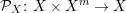 ${\mathcal{P}}_{X}:X\times X^{m}\rightarrow X$
is the usual projection. The final step is to replace the hand-crafted updating operators
${\mathcal{P}}_{X}:X\times X^{m}\rightarrow X$
is the usual projection. The final step is to replace the hand-crafted updating operators
 $\unicode[STIX]{x1D6E4}_{\unicode[STIX]{x1D703}_{k}}:X\times X^{m}\times X\rightarrow X$
with deep neural networks that then train the resulting
$\unicode[STIX]{x1D6E4}_{\unicode[STIX]{x1D703}_{k}}:X\times X^{m}\times X\rightarrow X$
with deep neural networks that then train the resulting
 ${\mathcal{R}}_{\unicode[STIX]{x1D703}}:Y\rightarrow X$
against unsupervised data as in (4.31).
${\mathcal{R}}_{\unicode[STIX]{x1D703}}:Y\rightarrow X$
against unsupervised data as in (4.31).
In inverse problem applications, the objective in (4.29) often has further structure that can be utilized. A typical example is (2.7), where the objective is of the form
 $$\begin{eqnarray}{\mathcal{J}}(f,g):={\mathcal{L}}({\mathcal{A}}(f),g)+{\mathcal{S}}_{\unicode[STIX]{x1D706}}(f).\end{eqnarray}$$
A wide range of iterative schemes that better utilize such a structure include updating in both
 $X$
(primal) and
$X$
(primal) and
 $Y$
(dual) spaces. These can be written abstractly as
$Y$
(dual) spaces. These can be written abstractly as
 $$\begin{eqnarray}\left\{\begin{array}{@{}ll@{}}(f^{0},g^{0})=(f_{0},g)\in X\times Y\text{ with }f_{0}\text{ chosen},\quad & \\ (f^{k+1},g^{k+1}):=\unicode[STIX]{x1D6E4}_{\unicode[STIX]{x1D703}_{k}}(f^{k},\mathbf{f}_{m_{1}}^{k},g^{k},\mathbf{g}_{m_{2}}^{k},[\unicode[STIX]{x2202}\!{\mathcal{A}}(f^{k})]^{\ast }(g^{k}),{\mathcal{A}}(f^{k}),\unicode[STIX]{x1D6FB}\!{\mathcal{S}}_{\unicode[STIX]{x1D706}}(f^{k}),)\quad \end{array}\right.\end{eqnarray}$$
for some updating operator
 $$\begin{eqnarray}\unicode[STIX]{x1D6E4}_{\unicode[STIX]{x1D703}_{k}}:X\times X^{m_{1}}\times Y\times Y^{m_{2}}\times X\times Y\times X\rightarrow X\times Y.\end{eqnarray}$$
Here,
 $m_{1},m_{2}$
is the memory in the
$m_{1},m_{2}$
is the memory in the
 $X$
- and
$X$
- and
 $Y$
-iterates, so
$Y$
-iterates, so
 $$\begin{eqnarray}\mathbf{f}_{m_{1}}^{k}=(f^{k-1},\ldots ,f^{k-m_{1}})\in X^{m_{1}}\quad \text{and}\quad \mathbf{g}_{m_{2}}^{k}=(g^{k-1},\ldots ,g^{k-m_{2}})\in Y^{m_{2}},\end{eqnarray}$$
with the convention that
 $f^{k-l}=f^{0}$
and
$f^{k-l}=f^{0}$
and
 $g^{k-l}=g$
whenever
$g^{k-l}=g$
whenever
 $k-l<0$
. Stopping and unrolling such a scheme after
$k-l<0$
. Stopping and unrolling such a scheme after
 $N$
iterates amounts to defining
$N$
iterates amounts to defining
 ${\mathcal{R}}_{\unicode[STIX]{x1D703}}:Y\rightarrow X$
with
${\mathcal{R}}_{\unicode[STIX]{x1D703}}:Y\rightarrow X$
with
 $\unicode[STIX]{x1D703}=(\unicode[STIX]{x1D703}_{1},\ldots ,\unicode[STIX]{x1D703}_{N})$
as
$\unicode[STIX]{x1D703}=(\unicode[STIX]{x1D703}_{1},\ldots ,\unicode[STIX]{x1D703}_{N})$
as
 $$\begin{eqnarray}{\mathcal{R}}_{\unicode[STIX]{x1D703}}(g):=({\mathcal{P}}_{X}\circ \unicode[STIX]{x1D6EC}_{\unicode[STIX]{x1D703}_{N}}\circ \ldots \circ \unicode[STIX]{x1D6EC}_{\unicode[STIX]{x1D703}_{1}})(f^{0},\mathbf{f}_{m_{1}}^{0},g,\mathbf{g}_{m_{2}}^{0}),\end{eqnarray}$$
where
 $\unicode[STIX]{x1D6EC}_{\unicode[STIX]{x1D703}_{k}}:X\times X^{m_{1}}\times Y\times Y^{m_{2}}\rightarrow X\times X^{m_{1}}\times Y\times Y^{m_{2}}$
for
$\unicode[STIX]{x1D6EC}_{\unicode[STIX]{x1D703}_{k}}:X\times X^{m_{1}}\times Y\times Y^{m_{2}}\rightarrow X\times X^{m_{1}}\times Y\times Y^{m_{2}}$
for
 $k=1,\ldots ,N$
is defined as
$k=1,\ldots ,N$
is defined as
 $$\begin{eqnarray}\unicode[STIX]{x1D6EC}_{\unicode[STIX]{x1D703}_{k}}(f,\mathbf{h},v,\mathbf{v}):=(\hat{f}_{\unicode[STIX]{x1D703}_{k}},\mathbf{h}^{\prime },\hat{v}_{\unicode[STIX]{x1D703}_{k}},\mathbf{v}^{\prime }),\end{eqnarray}$$
with
 $\mathbf{h}^{\prime }:=(h_{2},\ldots ,h_{m_{1}})\in X^{m_{1}-1}$
,
$\mathbf{h}^{\prime }:=(h_{2},\ldots ,h_{m_{1}})\in X^{m_{1}-1}$
,
 $\mathbf{v}^{\prime }:=(v_{2},\ldots ,v_{m_{2}})\in X^{m_{2}-1}$
, and
$\mathbf{v}^{\prime }:=(v_{2},\ldots ,v_{m_{2}})\in X^{m_{2}-1}$
, and
 $$\begin{eqnarray}(\hat{f}_{\unicode[STIX]{x1D703}_{k}},\hat{v}_{\unicode[STIX]{x1D703}_{k}}):=\unicode[STIX]{x1D6E4}_{\unicode[STIX]{x1D703}_{k}}(f,\mathbf{f},v,\mathbf{v},[\unicode[STIX]{x2202}\!{\mathcal{A}}(f)]^{\ast }(v),{\mathcal{A}}(f),\unicode[STIX]{x1D6FB}\!{\mathcal{S}}_{\unicode[STIX]{x1D706}}(f))\in X\times Y.\end{eqnarray}$$
In the above,
 ${\mathcal{P}}_{X}:X\times X^{m_{1}}\times Y\times Y^{m_{2}}\rightarrow X$
is the usual projection and, just as before, these hand-crafted updating operators are replaced with deep neural networks and the resulting deep neural network
${\mathcal{P}}_{X}:X\times X^{m_{1}}\times Y\times Y^{m_{2}}\rightarrow X$
is the usual projection and, just as before, these hand-crafted updating operators are replaced with deep neural networks and the resulting deep neural network
 ${\mathcal{R}}_{\unicode[STIX]{x1D703}}:Y\rightarrow X$
is trained against training data, for example as in (4.31) in the case with unsupervised data.
${\mathcal{R}}_{\unicode[STIX]{x1D703}}:Y\rightarrow X$
is trained against training data, for example as in (4.31) in the case with unsupervised data.
Likewise, in the setting where
 ${\mathcal{S}}_{\unicode[STIX]{x1D706}}:X\rightarrow \mathbb{R}$
in (4.35) is non-smooth, the prototype proximal-gradient scheme without memory reads as
${\mathcal{S}}_{\unicode[STIX]{x1D706}}:X\rightarrow \mathbb{R}$
in (4.35) is non-smooth, the prototype proximal-gradient scheme without memory reads as
 $$\begin{eqnarray}\left\{\begin{array}{@{}ll@{}}f^{k+1/2}:=\unicode[STIX]{x1D6EC}_{\unicode[STIX]{x1D703}_{k}^{1}}(f^{k},\unicode[STIX]{x1D6FB}_{\!f}{\mathcal{L}}({\mathcal{A}}(f^{k}),g)),\quad & \\ f^{k+1}:=\unicode[STIX]{x1D6EC}_{\unicode[STIX]{x1D703}_{k}^{2}}(f^{k},f^{k+1/2},\operatorname{prox}_{\unicode[STIX]{x1D6FE}{\mathcal{S}}_{\unicode[STIX]{x1D706}}}(f^{k+1/2})),\quad \end{array}\right.\end{eqnarray}$$
for updating operators
 $\unicode[STIX]{x1D6EC}_{\unicode[STIX]{x1D703}_{k}^{1}}:X\times X\rightarrow X$
and
$\unicode[STIX]{x1D6EC}_{\unicode[STIX]{x1D703}_{k}^{1}}:X\times X\rightarrow X$
and
 $\unicode[STIX]{x1D6EC}_{\unicode[STIX]{x1D703}_{k}^{2}}:X\times X\times X\rightarrow X$
. Now, just as before, one can terminate and unroll the above scheme after
$\unicode[STIX]{x1D6EC}_{\unicode[STIX]{x1D703}_{k}^{2}}:X\times X\times X\rightarrow X$
. Now, just as before, one can terminate and unroll the above scheme after
 $N$
iterates and replace the updating operators with deep neural networks. The resulting deep neural network
$N$
iterates and replace the updating operators with deep neural networks. The resulting deep neural network
 ${\mathcal{R}}_{\unicode[STIX]{x1D703}}:Y\rightarrow X$
, where
${\mathcal{R}}_{\unicode[STIX]{x1D703}}:Y\rightarrow X$
, where
 $\unicode[STIX]{x1D703}=(\unicode[STIX]{x1D703}_{1}^{1},\ldots ,\unicode[STIX]{x1D703}_{N}^{1},\unicode[STIX]{x1D703}_{1}^{2},\ldots ,\unicode[STIX]{x1D703}_{N}^{2})$
, is then trained against unsupervised data as in (4.31). Just as in the smooth case, it is furthermore possible to add memory and/or ‘break up’ the objective even further, the latter in order to better account for the structure in the problem. For example, variational methods for linear inverse problems often result in minimizing an objective of the form
$\unicode[STIX]{x1D703}=(\unicode[STIX]{x1D703}_{1}^{1},\ldots ,\unicode[STIX]{x1D703}_{N}^{1},\unicode[STIX]{x1D703}_{1}^{2},\ldots ,\unicode[STIX]{x1D703}_{N}^{2})$
, is then trained against unsupervised data as in (4.31). Just as in the smooth case, it is furthermore possible to add memory and/or ‘break up’ the objective even further, the latter in order to better account for the structure in the problem. For example, variational methods for linear inverse problems often result in minimizing an objective of the form
 $$\begin{eqnarray}{\mathcal{J}}(f,g):={\mathcal{S}}_{\unicode[STIX]{x1D706}}(f)+\mathop{\sum }_{i=1}^{m}{\mathcal{L}}_{i}({\mathcal{A}}_{i}(f),g_{i})\end{eqnarray}$$
where
 ${\mathcal{A}}_{i}:X\rightarrow Y_{i}$
are linear and
${\mathcal{A}}_{i}:X\rightarrow Y_{i}$
are linear and
 ${\mathcal{S}}_{\unicode[STIX]{x1D706}}:X\rightarrow [-\infty ,\infty ]$
and
${\mathcal{S}}_{\unicode[STIX]{x1D706}}:X\rightarrow [-\infty ,\infty ]$
and
 ${\mathcal{L}}_{i}:Y_{i}\times Y_{i}\rightarrow [-\infty ,\infty ]$
are proper, convex and lower semicontinuous. One can then consider unrolling iterative schemes that utilize this structure, such as operator splitting techniques: see Eckstein and Bertsekas (Reference Eckstein and Bertsekas1992), Beck and Teboulle (Reference Beck and Teboulle2009), Chambolle and Pock (Reference Chambolle and Pock2011), Boyd et al. (Reference Boyd, Parikh, Chu, Peleato and Eckstein2011), Combettes and Pesquet (Reference Combettes, Pesquet and Bauschke2011, Reference Combettes and Pesquet2012), He and Yuan (Reference He and Yuan2012), Boţ and Hendrich (Reference Boţ and Hendrich2013), Boţ and Csetnek (Reference Boţ and Csetnek2015), Ko, Yu and Won (Reference Ko, Yu and Won2017), Latafat and Patrinos (Reference Latafat and Patrinos2017) and Bauschke and Combettes (Reference Bauschke and Combettes2017).
${\mathcal{L}}_{i}:Y_{i}\times Y_{i}\rightarrow [-\infty ,\infty ]$
are proper, convex and lower semicontinuous. One can then consider unrolling iterative schemes that utilize this structure, such as operator splitting techniques: see Eckstein and Bertsekas (Reference Eckstein and Bertsekas1992), Beck and Teboulle (Reference Beck and Teboulle2009), Chambolle and Pock (Reference Chambolle and Pock2011), Boyd et al. (Reference Boyd, Parikh, Chu, Peleato and Eckstein2011), Combettes and Pesquet (Reference Combettes, Pesquet and Bauschke2011, Reference Combettes and Pesquet2012), He and Yuan (Reference He and Yuan2012), Boţ and Hendrich (Reference Boţ and Hendrich2013), Boţ and Csetnek (Reference Boţ and Csetnek2015), Ko, Yu and Won (Reference Ko, Yu and Won2017), Latafat and Patrinos (Reference Latafat and Patrinos2017) and Bauschke and Combettes (Reference Bauschke and Combettes2017).
A natural question is to investigate the error in using
 ${\mathcal{R}}_{\unicode[STIX]{x1D703}}$
to approximate
${\mathcal{R}}_{\unicode[STIX]{x1D703}}$
to approximate
 ${\mathcal{R}}$
as a function of
${\mathcal{R}}$
as a function of
 $N$
and properties of the unsupervised training data. Such estimates, which are referred to as time–accuracy trade-offs, have been proved for LISTA (Section 4.9.2) by Giryes, Eldar, Bronstein and Sapiro (Reference Giryes, Eldar, Bronstein and Sapiro2017); see also Oymak and Soltanolkotabi (Reference Oymak and Soltanolkotabi2017) for further development along these lines. Another related type of investigation has been pursued by Banert et al. (Reference Banert, Ringh, Adler, Karlsson and Öktem2018), who derive conditions on the unrolled iterative scheme that is terminated after
$N$
and properties of the unsupervised training data. Such estimates, which are referred to as time–accuracy trade-offs, have been proved for LISTA (Section 4.9.2) by Giryes, Eldar, Bronstein and Sapiro (Reference Giryes, Eldar, Bronstein and Sapiro2017); see also Oymak and Soltanolkotabi (Reference Oymak and Soltanolkotabi2017) for further development along these lines. Another related type of investigation has been pursued by Banert et al. (Reference Banert, Ringh, Adler, Karlsson and Öktem2018), who derive conditions on the unrolled iterative scheme that is terminated after
 $N$
iterates, so that training this yields a scheme that is convergent in the limit. It turns out that imposing such convergence constraints has only a minor impact on the performance at
$N$
iterates, so that training this yields a scheme that is convergent in the limit. It turns out that imposing such convergence constraints has only a minor impact on the performance at
 $N$
iterates. Furthermore, it improves the generalization properties, that is, one can use the same trained solver even when the objective is slightly changed, for example by considering a different forward operator.
$N$
iterates. Furthermore, it improves the generalization properties, that is, one can use the same trained solver even when the objective is slightly changed, for example by considering a different forward operator.
To summarize, the iterative update in most schemes for solving optimization problems has the structure of a composition of (possibly multiple) affine operations followed by a non-linear operation. If each iterate is identified with a layer and the non-linear operation plays the role of an activation function, e.g.
 ${\mathcal{S}}_{\unicode[STIX]{x1D706}}(f)=\unicode[STIX]{x1D706}\Vert f\Vert$
, then
${\mathcal{S}}_{\unicode[STIX]{x1D706}}(f)=\unicode[STIX]{x1D706}\Vert f\Vert$
, then
 $\operatorname{prox}_{\unicode[STIX]{x1D706}{\mathcal{S}}}$
corresponds to soft thresholding, which in turn is very close to the well-known ReLU activation function. In this way the iterative scheme stopped after
$\operatorname{prox}_{\unicode[STIX]{x1D706}{\mathcal{S}}}$
corresponds to soft thresholding, which in turn is very close to the well-known ReLU activation function. In this way the iterative scheme stopped after
 $N$
steps can be represented via a neural network with an architecture that is adapted to that iterative scheme.
$N$
steps can be represented via a neural network with an architecture that is adapted to that iterative scheme.
4.9.2 Learned Iterative Soft-Thresholding Algorithm (LISTA)
LISTA is the earliest example of unrolling an optimization scheme and it was first introduced in Gregor and LeCun (Reference Gregor and LeCun2010). It is the abstract unrolling scheme in Section 4.9.1 adapted to the specific case of ISTA iterates (Section A.3). This results in a fully connected network with
 $N$
-internal layers of identical size that is adapted to evaluating the solution operator for the following convex non-smooth optimization problem:
$N$
-internal layers of identical size that is adapted to evaluating the solution operator for the following convex non-smooth optimization problem:
 $$\begin{eqnarray}{\mathcal{R}}(g):={\mathcal{E}}^{\ast }(\hat{\unicode[STIX]{x1D709}}),\end{eqnarray}$$
where
Such optimization problems arise as the convex relaxation of (2.20), which is sparsity-promoting regularization of an ill-posed linear inverse problem (Section 2.7).
The ISTA iterative scheme for evaluating
 ${\mathcal{R}}$
reads as
${\mathcal{R}}$
reads as
 $$\begin{eqnarray}\unicode[STIX]{x1D709}^{n+1}=\operatorname{prox}_{\unicode[STIX]{x1D706}\unicode[STIX]{x1D70F}\Vert \cdot \Vert _{1}}=S_{\unicode[STIX]{x1D706}\unicode[STIX]{x1D70F}}[\unicode[STIX]{x1D70F}{\mathcal{A}}_{{\mathcal{E}}^{\ast }}^{\ast }g+(\text{id}-\unicode[STIX]{x1D70F}{\mathcal{A}}_{{\mathcal{E}}^{\ast }}^{\ast }{\mathcal{A}}_{{\mathcal{E}}^{\ast }})\unicode[STIX]{x1D709}^{n}],\end{eqnarray}$$
where
 $0<\unicode[STIX]{x1D70F}<2/L$
is the step length approximated by the reciprocal of the Lipschitz constant of
$0<\unicode[STIX]{x1D70F}<2/L$
is the step length approximated by the reciprocal of the Lipschitz constant of
 ${\mathcal{A}}_{{\mathcal{E}}^{\ast }}$
, and
${\mathcal{A}}_{{\mathcal{E}}^{\ast }}$
, and
 $S$
is the shrinkage operator (see Section A.3). Now the insight is to recognize
$S$
is the shrinkage operator (see Section A.3). Now the insight is to recognize
 $b_{k}(g):=\unicode[STIX]{x1D70F}_{k}{\mathcal{A}}_{{\mathcal{E}}^{\ast }}^{\ast }g$
as a bias,
$b_{k}(g):=\unicode[STIX]{x1D70F}_{k}{\mathcal{A}}_{{\mathcal{E}}^{\ast }}^{\ast }g$
as a bias,
 $W_{k}:=(\text{id}-\unicode[STIX]{x1D70F}_{k}{\mathcal{A}}_{{\mathcal{E}}^{\ast }}^{\ast }{\mathcal{A}}_{{\mathcal{E}}^{\ast }})$
as a fixed linear operator and
$W_{k}:=(\text{id}-\unicode[STIX]{x1D70F}_{k}{\mathcal{A}}_{{\mathcal{E}}^{\ast }}^{\ast }{\mathcal{A}}_{{\mathcal{E}}^{\ast }})$
as a fixed linear operator and
 $\unicode[STIX]{x1D713}_{k}=S_{\unicode[STIX]{x1D706}\unicode[STIX]{x1D70F}_{k}}$
as a pointwise non-linearity. Note that
$\unicode[STIX]{x1D713}_{k}=S_{\unicode[STIX]{x1D706}\unicode[STIX]{x1D70F}_{k}}$
as a pointwise non-linearity. Note that
 $W_{k}$
is symmetric positive definite by construction. Assuming a fixed iteration number
$W_{k}$
is symmetric positive definite by construction. Assuming a fixed iteration number
 $N$
, we may write the approximation to (4.40) as
$N$
, we may write the approximation to (4.40) as
 $$\begin{eqnarray}\left\{\begin{array}{@{}ll@{}}\unicode[STIX]{x1D709}^{(0)}\in \unicode[STIX]{x1D6EF}\text{given}\quad & \\ \unicode[STIX]{x1D709}^{(k)}=\unicode[STIX]{x1D713}(W_{k}\unicode[STIX]{x1D709}^{(k-1)}+b_{k}(g))\quad & \end{array}\right.\quad \text{for }k=1,\ldots ,N.\end{eqnarray}$$
In unrolled form, the above defines
 ${\mathcal{R}}_{\unicode[STIX]{x1D703}}:Y\rightarrow \unicode[STIX]{x1D6EF}$
with
${\mathcal{R}}_{\unicode[STIX]{x1D703}}:Y\rightarrow \unicode[STIX]{x1D6EF}$
with
 $\unicode[STIX]{x1D703}_{k}:=(\unicode[STIX]{x1D713},\unicode[STIX]{x1D70F}_{k},W_{k},b_{k})$
as
$\unicode[STIX]{x1D703}_{k}:=(\unicode[STIX]{x1D713},\unicode[STIX]{x1D70F}_{k},W_{k},b_{k})$
as
 $$\begin{eqnarray}{\mathcal{R}}_{\unicode[STIX]{x1D703}}:=(\unicode[STIX]{x1D6EC}_{\unicode[STIX]{x1D703}_{N}}\circ \ldots \circ \unicode[STIX]{x1D6EC}_{\unicode[STIX]{x1D703}_{1}})(\unicode[STIX]{x1D709}^{(0)})\end{eqnarray}$$
where
 $\unicode[STIX]{x1D6EC}_{\unicode[STIX]{x1D703}_{k}}:\unicode[STIX]{x1D6EF}\rightarrow \unicode[STIX]{x1D6EF}$
is
$\unicode[STIX]{x1D6EC}_{\unicode[STIX]{x1D703}_{k}}:\unicode[STIX]{x1D6EF}\rightarrow \unicode[STIX]{x1D6EF}$
is
 $\unicode[STIX]{x1D6EC}_{\unicode[STIX]{x1D703}_{k}}:=\unicode[STIX]{x1D713}_{k}\circ (W_{k}+b_{k}(g)\text{id})$
. This is precisely the form of a feed-forward network with
$\unicode[STIX]{x1D6EC}_{\unicode[STIX]{x1D703}_{k}}:=\unicode[STIX]{x1D713}_{k}\circ (W_{k}+b_{k}(g)\text{id})$
. This is precisely the form of a feed-forward network with
 $N$
layers, each with identical fixed affine map
$N$
layers, each with identical fixed affine map
 ${\mathcal{W}}_{k}(\unicode[STIX]{x1D709}):=W_{k}\unicode[STIX]{x1D709}+b_{k}$
; the activation function
${\mathcal{W}}_{k}(\unicode[STIX]{x1D709}):=W_{k}\unicode[STIX]{x1D709}+b_{k}$
; the activation function
 $\unicode[STIX]{x1D713}_{k}:=S_{\unicode[STIX]{x1D706}\unicode[STIX]{x1D70F}_{k}}$
is given by the shrinkage operator (see Section A.3).
$\unicode[STIX]{x1D713}_{k}:=S_{\unicode[STIX]{x1D706}\unicode[STIX]{x1D70F}_{k}}$
is given by the shrinkage operator (see Section A.3).
Remark 4.9. The expression given in (4.42) has the form of an encoder
 $\unicode[STIX]{x1D6F9}_{W}:Y\rightarrow \unicode[STIX]{x1D6EF}$
for a fixed dictionary given by
$\unicode[STIX]{x1D6F9}_{W}:Y\rightarrow \unicode[STIX]{x1D6EF}$
for a fixed dictionary given by
 $W$
.
$W$
.
The affine maps between the layers are assumed to be identical. LISTA then trains
 $W$
and potentially
$W$
and potentially
 $\unicode[STIX]{x1D713}$
on some given unsupervised training data by solving (4.31). The derivation of Gregor and LeCun (Reference Gregor and LeCun2010) is framed in terms of learning a sparse encoder. Here we rephrase the idea in terms of a reconstruction problem and a learned decoder as follows.
$\unicode[STIX]{x1D713}$
on some given unsupervised training data by solving (4.31). The derivation of Gregor and LeCun (Reference Gregor and LeCun2010) is framed in terms of learning a sparse encoder. Here we rephrase the idea in terms of a reconstruction problem and a learned decoder as follows.
Lemma 4.10. Let
 $\unicode[STIX]{x1D6F9}_{W}^{\dagger }:\unicode[STIX]{x1D6EF}\rightarrow X$
denote a fully connected network with input
$\unicode[STIX]{x1D6F9}_{W}^{\dagger }:\unicode[STIX]{x1D6EF}\rightarrow X$
denote a fully connected network with input
 $\unicode[STIX]{x1D709}^{0}$
and
$\unicode[STIX]{x1D709}^{0}$
and
 $N$
-internal layers. Furthermore, assume that the activation function is identical to a proximal mapping for a convex functional
$N$
-internal layers. Furthermore, assume that the activation function is identical to a proximal mapping for a convex functional
 $\unicode[STIX]{x1D70F}\unicode[STIX]{x1D706}{\mathcal{S}}:\unicode[STIX]{x1D6EF}\rightarrow \mathbb{R}$
. Also, let
$\unicode[STIX]{x1D70F}\unicode[STIX]{x1D706}{\mathcal{S}}:\unicode[STIX]{x1D6EF}\rightarrow \mathbb{R}$
. Also, let
 $W$
be restricted so that
$W$
be restricted so that
 $\text{id}-W$
is positive definite, i.e. there exists a matrix
$\text{id}-W$
is positive definite, i.e. there exists a matrix
 $B$
such that
$B$
such that
 $$\begin{eqnarray}\text{id}-W=\unicode[STIX]{x1D70F}B^{\ast }B.\end{eqnarray}$$
Finally, fix the bias term as
 $b=\unicode[STIX]{x1D70F}B^{\ast }g$
. Then
$b=\unicode[STIX]{x1D70F}B^{\ast }g$
. Then
 $\unicode[STIX]{x1D6F9}_{W}^{\dagger }(\unicode[STIX]{x1D709})$
is the
$\unicode[STIX]{x1D6F9}_{W}^{\dagger }(\unicode[STIX]{x1D709})$
is the
 $N$
th iterate of an ISTA scheme with starting value
$N$
th iterate of an ISTA scheme with starting value
 $\unicode[STIX]{x1D709}^{(0)}$
for minimizing
$\unicode[STIX]{x1D709}^{(0)}$
for minimizing
 $$\begin{eqnarray}{\mathcal{J}}_{B}(\unicode[STIX]{x1D709})=\frac{1}{2}\Vert B\unicode[STIX]{x1D709}-g\Vert ^{2}+\unicode[STIX]{x1D706}{\mathcal{S}}(\unicode[STIX]{x1D709}).\end{eqnarray}$$
Note that the connection to ISTA is only given when the weights are the same across layers. The conclusion in the lemma follows directly from (A.10). In this sense, training a decoder network
 $\unicode[STIX]{x1D6F9}_{W}^{\dagger }$
by minimizing
$\unicode[STIX]{x1D6F9}_{W}^{\dagger }$
by minimizing
 $$\begin{eqnarray}\frac{1}{2}\Vert {\mathcal{A}}\unicode[STIX]{x1D6F9}_{W}^{\dagger }(\unicode[STIX]{x1D709})-g\Vert ^{2}\end{eqnarray}$$
with respect to
 $W$
, and computing
$W$
, and computing
 $\hat{f}=\unicode[STIX]{x1D6F9}_{W}^{\dagger }(\unicode[STIX]{x1D709})$
is equivalent to computing
$\hat{f}=\unicode[STIX]{x1D6F9}_{W}^{\dagger }(\unicode[STIX]{x1D709})$
is equivalent to computing
 $\hat{B}$
by minimizing a Tikhonov functional of the form (4.43) with respect to
$\hat{B}$
by minimizing a Tikhonov functional of the form (4.43) with respect to
 $B$
, then computing
$B$
, then computing
 $\hat{f}:=\unicode[STIX]{x1D6F9}_{W}^{\dagger }(\hat{B})$
as a solution to the inverse problem. Following these arguments, one can rephrase LISTA as a concept for learning the discrepancy term in a classical Tikhonov functional.
$\hat{f}:=\unicode[STIX]{x1D6F9}_{W}^{\dagger }(\hat{B})$
as a solution to the inverse problem. Following these arguments, one can rephrase LISTA as a concept for learning the discrepancy term in a classical Tikhonov functional.
Remark 4.11. The restriction of activation functions to proximal mappings is not as severe as it might look at first glance. For example, as already mentioned in Section 4.9.1, ReLU is the proximal mapping for the indicator function of positive real numbers and soft shrinkage is the proximal mapping for the modulus function.
4.9.3 Learned proximal operators
Just as with LISTA, the learned proximal operator approach is the abstract unrolling scheme in Section 4.9.1 adapted to the specific case of unrolling operator-splitting approaches, such as proximal gradient (PG), primaldual hybrid gradient (PDHG) or ADMM; see also Section A and Chambolle and Pock (Reference Chambolle and Pock2016).
More precisely, consider the variational regularization that minimizes the functional in (4.35) under the Gaussian noise log-likelihood model with covariance
 $\unicode[STIX]{x1D6F4}$
and a non-smooth regularizer, that is,
$\unicode[STIX]{x1D6F4}$
and a non-smooth regularizer, that is,
 $$\begin{eqnarray}{\mathcal{R}}(g):=\hat{f},\end{eqnarray}$$
where
 $$\begin{eqnarray}\hat{f}:=\text{arg}\,\text{min}\{\unicode[STIX]{x1D706}{\mathcal{S}}(f)+\Vert {\mathcal{A}}(f)-g\Vert _{\unicode[STIX]{x1D6F4}^{-1}}^{2}\}\end{eqnarray}$$
and
 ${\mathcal{S}}:X\rightarrow \mathbb{R}$
is non-smooth. Our aim is to approximate
${\mathcal{S}}:X\rightarrow \mathbb{R}$
is non-smooth. Our aim is to approximate
 ${\mathcal{R}}(g)$
in (4.44) by a deep neural network that is obtained by unrolling a suitable scheme.
${\mathcal{R}}(g)$
in (4.44) by a deep neural network that is obtained by unrolling a suitable scheme.
Unrolling iterates of a PG method (Section A.2) and replacing the proximal operator with a learned operator yields
 $$\begin{eqnarray}{\mathcal{R}}_{\unicode[STIX]{x1D703}}(g):=f^{N},\end{eqnarray}$$
where
 $$\begin{eqnarray}f^{k+1}:=\unicode[STIX]{x1D6EC}_{\unicode[STIX]{x1D703}}(f^{k}+\unicode[STIX]{x1D70F}{\mathcal{A}}^{\ast }\unicode[STIX]{x1D6F4}^{-1}({\mathcal{A}}f^{k}-g)).\end{eqnarray}$$
In the above,
 $\unicode[STIX]{x1D6EC}_{\unicode[STIX]{x1D703}}:X\rightarrow X$
is a deep neural network that replaces the proximal of
$\unicode[STIX]{x1D6EC}_{\unicode[STIX]{x1D703}}:X\rightarrow X$
is a deep neural network that replaces the proximal of
 ${\mathcal{S}}$
in (4.44). Similarly, the ADMM framework (Section A.4) has the augmented Lagrangian
${\mathcal{S}}$
in (4.44). Similarly, the ADMM framework (Section A.4) has the augmented Lagrangian
 $$\begin{eqnarray}{\mathcal{L}}(f,h,u)=\frac{1}{2}\Vert {\mathcal{A}}(f)-g\Vert _{\unicode[STIX]{x1D6F4}^{-1}}^{2}+\unicode[STIX]{x1D706}{\mathcal{S}}(h)+\frac{\unicode[STIX]{x1D6FD}}{2}\biggl\|f-h+\frac{1}{\unicode[STIX]{x1D6FD}}u\biggr\|_{2}^{2}-\frac{1}{2\unicode[STIX]{x1D6FD}}\Vert u\Vert _{2}^{2},\end{eqnarray}$$
which results in
 ${\mathcal{R}}_{\unicode[STIX]{x1D703}}(g):=f^{N}$
, where
${\mathcal{R}}_{\unicode[STIX]{x1D703}}(g):=f^{N}$
, where
 $$\begin{eqnarray}\displaystyle & & \displaystyle \displaystyle f^{k+1}:=({\mathcal{A}}^{\ast }\unicode[STIX]{x1D6F4}^{-1}{\mathcal{A}}+\unicode[STIX]{x1D6FD}\text{id})^{-1}({\mathcal{A}}^{\ast }\unicode[STIX]{x1D6F4}^{-1}({\mathcal{A}}(f^{k})-g)+\unicode[STIX]{x1D6FD}(f^{k}-h^{k})+u^{k}),\end{eqnarray}$$
 $$\begin{eqnarray}\displaystyle & & \displaystyle \displaystyle h^{k+1}:=\unicode[STIX]{x1D6EC}_{\unicode[STIX]{x1D703}}\biggl(f^{k+1}+\frac{1}{\unicode[STIX]{x1D6FD}}u^{k}\biggr),\end{eqnarray}$$
 $$\begin{eqnarray}\displaystyle & & \displaystyle \displaystyle u^{k+1}:=u^{k}+\unicode[STIX]{x1D6FD}(f^{k+1}-h^{k+1}),\end{eqnarray}$$
where the general expression for the proximal operator of the log-likelihood from (A.12) has the direct form (4.47), and the general expression for the proximal operator of
 ${\mathcal{S}}$
from (A.13) is replaced with a network
${\mathcal{S}}$
from (A.13) is replaced with a network
 $\unicode[STIX]{x1D6EC}_{\unicode[STIX]{x1D703}}:X\rightarrow X$
in (4.48).
$\unicode[STIX]{x1D6EC}_{\unicode[STIX]{x1D703}}:X\rightarrow X$
in (4.48).
This compares to other
 $P^{3}$
approaches (Section 4.6) using a denoising method such as BM3D in place of the proximal operator. An important point noted in Meinhardt et al. (Reference Meinhardt, Moeller, Hazirbas and Cremers2017) is that by choosing
$P^{3}$
approaches (Section 4.6) using a denoising method such as BM3D in place of the proximal operator. An important point noted in Meinhardt et al. (Reference Meinhardt, Moeller, Hazirbas and Cremers2017) is that by choosing
 $\unicode[STIX]{x1D6FD}=1$
in (4.46), the networks do not need to be retrained on different noise levels if they can be considered as a scaling of the likelihood term. Related work includes ‘deep image demosaicing’ using a cascade of convolutional residual denoising networks (Kokkinos and Lefkimmiatis Reference Kokkinos and Lefkimmiatis2018, Lefkimmiatis Reference Lefkimmiatis2017), which includes learning of the activation function.
$\unicode[STIX]{x1D6FD}=1$
in (4.46), the networks do not need to be retrained on different noise levels if they can be considered as a scaling of the likelihood term. Related work includes ‘deep image demosaicing’ using a cascade of convolutional residual denoising networks (Kokkinos and Lefkimmiatis Reference Kokkinos and Lefkimmiatis2018, Lefkimmiatis Reference Lefkimmiatis2017), which includes learning of the activation function.
A related method is that of Chang et al. (Reference Chang, Li, Póczos, Kumar and Sankaranarayanan2017), who propose a general framework that implicitly learns a signal prior and a projection operator from a large image dataset and is predicated on the ADMM framework (Section A.4). In place of an ‘ideal’ prior defined as the indicator function
 $\mathbb{I}_{X_{0}}:X\rightarrow \mathbb{R}$
on the set of natural images
$\mathbb{I}_{X_{0}}:X\rightarrow \mathbb{R}$
on the set of natural images
 $X_{0}\subset X$
and its proximal operator, they make use of a trained classifier
$X_{0}\subset X$
and its proximal operator, they make use of a trained classifier
 ${\mathcal{D}}:X\rightarrow [0,1]$
and a learned projection function
${\mathcal{D}}:X\rightarrow [0,1]$
and a learned projection function
 ${\mathcal{P}}$
that maps an estimated
${\mathcal{P}}$
that maps an estimated
 $\hat{f}\in X$
to the set defined by the classifier; the learned
$\hat{f}\in X$
to the set defined by the classifier; the learned
 ${\mathcal{P}}$
then replaces the proximal operator within the ADMM updates. They identify sufficient conditions for the convergence of the non-convex ADMM with the proposed projection operator, and use these conditions as guidelines to design the proposed projection network. They show that it is inefficient at solving generic linear inverse problems with state-of-the-art methods using specially trained networks. Experimental results also show that these are prone to being affected by changes in the linear operators and noise in the linear measurements. In contrast, the proposed method is more robust to these factors. Results are shown for the trained network applied to several problems including compressive sensing, denoising, in-painting (random pixels and block-wise) and super-resolution, and to different databases including MNIST, MS-Celeb-1M dataset and the ImageNet dataset.
${\mathcal{P}}$
then replaces the proximal operator within the ADMM updates. They identify sufficient conditions for the convergence of the non-convex ADMM with the proposed projection operator, and use these conditions as guidelines to design the proposed projection network. They show that it is inefficient at solving generic linear inverse problems with state-of-the-art methods using specially trained networks. Experimental results also show that these are prone to being affected by changes in the linear operators and noise in the linear measurements. In contrast, the proposed method is more robust to these factors. Results are shown for the trained network applied to several problems including compressive sensing, denoising, in-painting (random pixels and block-wise) and super-resolution, and to different databases including MNIST, MS-Celeb-1M dataset and the ImageNet dataset.
4.9.4 Summary and concluding remarks on unrolling
The idea of unrolling can be seen as constructing a deep neural network architecture. Here we used it to approximate solution operators to optimization problems, which are defined implicitly through an iterative optimization solver. This principle can, however, be applied in a much wider context and it also establishes a link between numerical analysis and deep learning.
For example, the learned iterative scheme (Section 5.1.4) uses unrolling to construct a deep learning architecture for the solution of an inverse problem that incorporates a forward operator and the adjoint of its derivative. Another example of using unrolling is that of Gilton, Ongie and Willett (Reference Gilton, Ongie and Willett2019), who construct a deep neural network by unrolling a truncated Neumann series for the inverse of a linear operator. This is used to successfully solve inverse problems with a linear forward operator. Gilton et al. claim that the resulting Neumann network architecture outperforms functional analytic approaches (Section 2), model-free deep learning approaches (Section 5.1.3) and state-of-the-art learned iterative schemes (Section 5.1.4) on standard datasets.
One can also unroll iterative schemes for solving PDEs, as shown by Hsieh et al. (Reference Hsieh, Zhao, Eismann, Mirabella and Ermon2019), who unroll an iterative solver tailored to a PDE and modify the updates using a deep neural network. A key part of their approach is ensuring that the learned scheme has convergence guarantees. See also Rizzuti, Siahkoohi and Herrmann (Reference Rizzuti, Siahkoohi and Herrmann2019) for a similar approach to solving the Helmholtz equation.
Finally, we also mention Ingraham, Riesselman, Sander and Marks (Reference Ingraham, Riesselman, Sander and Marks2019), who unroll a Monte Carlo simulation as a model for protein folding. They compose a neural energy function with a novel and efficient simulator based on Langevin dynamics to build an end-to-end-differentiable model of atomic protein structure given amino acid sequence information.
4.10 Deep inverse priors
Deep inverse priors (DIPs) generalize deep image priors that were recently introduced in Ulyanov, Vedaldi and Lempitsky (Reference Ulyanov, Vedaldi and Lempitsky2018) for some image processing tasks. We emphasize that deep inverse priors (DIPs) do not use a learned prior in the sense used so far in this paper. Deep inverse priors (DIPs), as we will see, more closely resemble non-linear Landweber schemes, but with a partly learned likelihood given by a trained neural network.
The choice of network design is crucial: it is assumed to provide a structural prior for the parameters or images to be reconstructed. More precisely, one assumes that the structure of a generator network is sufficient to capture most of the low-level image statistics prior to any learning. During the training of the network, more and more detailed information is added and an appropriate stopping criterion is essential to avoiding overfitting. In particular, a randomly initialized neural network can be used with excellent results in standard inverse problems such as denoising, super-resolution and in-painting.
For linear operators in a finite-dimensional setting, the task is to train a decoder network
 $\unicode[STIX]{x1D6F9}_{\unicode[STIX]{x1D703}}^{\dagger }:\unicode[STIX]{x1D6EF}\rightarrow X$
with fixed input
$\unicode[STIX]{x1D6F9}_{\unicode[STIX]{x1D703}}^{\dagger }:\unicode[STIX]{x1D6EF}\rightarrow X$
with fixed input
 $\unicode[STIX]{x1D709}_{0}\in \unicode[STIX]{x1D6EF}$
. The reconstruction operator
$\unicode[STIX]{x1D709}_{0}\in \unicode[STIX]{x1D6EF}$
. The reconstruction operator
 ${\mathcal{R}}:Y\rightarrow X$
is now given as the output of this decoder, that is,
${\mathcal{R}}:Y\rightarrow X$
is now given as the output of this decoder, that is,
 $$\begin{eqnarray}{\mathcal{R}}(g):=\unicode[STIX]{x1D6F9}_{\widehat{\unicode[STIX]{x1D703}}(g)}^{\dagger }(\unicode[STIX]{x1D709}_{0}),\end{eqnarray}$$
where
At the core of the DIP approach is the assumption that one can construct a (decoder) network
 $\unicode[STIX]{x1D6F9}_{\unicode[STIX]{x1D703}}^{\dagger }:\unicode[STIX]{x1D6EF}\rightarrow X$
which outputs elements in
$\unicode[STIX]{x1D6F9}_{\unicode[STIX]{x1D703}}^{\dagger }:\unicode[STIX]{x1D6EF}\rightarrow X$
which outputs elements in
 $X$
, which are close to or have a high probability of belonging to the set of feasible parameters.
$X$
, which are close to or have a high probability of belonging to the set of feasible parameters.
We emphasize that the training is with respect to
 $\unicode[STIX]{x1D703}$
: the input
$\unicode[STIX]{x1D703}$
: the input
 $\unicode[STIX]{x1D709}_{0}$
is kept fixed. Furthermore, machine learning approaches generally use large sets of training data, so it is somewhat surprising that deep image priors are trained on a single data set
$\unicode[STIX]{x1D709}_{0}$
is kept fixed. Furthermore, machine learning approaches generally use large sets of training data, so it is somewhat surprising that deep image priors are trained on a single data set
 $g$
. In summary, the main ingredients of deep inverse priors (DIPs) are a single data set, a well-chosen network architecture and a stopping criterion for terminating the training process (Ulyanov et al.
Reference Ulyanov, Vedaldi and Lempitsky2018).
$g$
. In summary, the main ingredients of deep inverse priors (DIPs) are a single data set, a well-chosen network architecture and a stopping criterion for terminating the training process (Ulyanov et al.
Reference Ulyanov, Vedaldi and Lempitsky2018).
One might assume that the network architecture
 $\unicode[STIX]{x1D6F9}_{\unicode[STIX]{x1D703}}^{\dagger }$
would need to incorporate rather specific details about the forward operator
$\unicode[STIX]{x1D6F9}_{\unicode[STIX]{x1D703}}^{\dagger }$
would need to incorporate rather specific details about the forward operator
 ${\mathcal{A}}$
, or even more importantly about the prior distribution
${\mathcal{A}}$
, or even more importantly about the prior distribution
 $\unicode[STIX]{x1D6F1}_{\text{prior}}$
of feasible model parameters. This seems not to be the case: empirical evidence suggests that rather generic network architectures work for different inverse problems, and the obtained numerical results demonstrate the potential of DIP approaches for large-scale inverse problems such as MPI.
$\unicode[STIX]{x1D6F1}_{\text{prior}}$
of feasible model parameters. This seems not to be the case: empirical evidence suggests that rather generic network architectures work for different inverse problems, and the obtained numerical results demonstrate the potential of DIP approaches for large-scale inverse problems such as MPI.
So far, investigations related to DIP have been predominantly experimental and mostly restricted to problems that do not fall within the class of ill-posed inverse problems. However, some work has been done in the context of inverse problems: for example, Van Veen et al. (Reference Van Veen, Jalal, Price, Vishwanath and Dimakis2018) consider the DIP approach to solve an inverse problem with a linear forward operator. They introduce a novel learned regularization technique which further reduces the number of measurements required to achieve a given reconstruction error. An approach similar to DIP is considered by Gupta et al. (Reference Gupta, Jin, Nguyen, McCann and Unser2018) for CT reconstruction. Here one regularizes by projection onto a convex set (see Gupta et al. Reference Gupta, Jin, Nguyen, McCann and Unser2018, equation (3)) and the projector is constructed by training a U-Net against unsupervised data. Gupta et al. (Reference Gupta, Jin, Nguyen, McCann and Unser2018, Theorem 3) also provide guarantees for convergence to a local minimum.
We now briefly summarize the known theoretical foundations of DIP for inverse problems based on the recent paper by Dittmer, Kluth, Maass and Baguer (Reference Dittmer, Kluth, Maass and Baguer2018), who analyse and prove that certain network architectures in combination with suitable stopping rules do indeed lead to regularization schemes, which lead to the notion of ‘regularization by architecture’. We also include numerical results for the integration operator; more complex results for MPI are presented in Section 7.5.
4.10.1 DIP with a trivial generator
To better understand the regularizing properties of DIP, we begin by considering a trivial generator that simply takes a scalar value of unity on a single node (i.e.
 $\unicode[STIX]{x1D709}_{0}=1$
) and outputs an element
$\unicode[STIX]{x1D709}_{0}=1$
) and outputs an element
 $h\in X$
, that is,
$h\in X$
, that is,
 $\unicode[STIX]{x1D6F9}_{\unicode[STIX]{x1D703}}^{\dagger }(\unicode[STIX]{x1D709}_{0})=h$
independently of
$\unicode[STIX]{x1D6F9}_{\unicode[STIX]{x1D703}}^{\dagger }(\unicode[STIX]{x1D709}_{0})=h$
independently of
 $\unicode[STIX]{x1D709}_{0}$
. This implies simply that the network is a single layer with the value
$\unicode[STIX]{x1D709}_{0}$
. This implies simply that the network is a single layer with the value
 $\unicode[STIX]{x1D703}=h$
, without any bias term or non-linear activation function. Then, the reconstruction operator in (4.50) reads as
$\unicode[STIX]{x1D703}=h$
, without any bias term or non-linear activation function. Then, the reconstruction operator in (4.50) reads as
 ${\mathcal{R}}(g)=\widehat{\unicode[STIX]{x1D703}}$
, where
${\mathcal{R}}(g)=\widehat{\unicode[STIX]{x1D703}}$
, where
In this setting
 $\unicode[STIX]{x1D703}$
can be directly identified with an element in
$\unicode[STIX]{x1D703}$
can be directly identified with an element in
 $X$
(and
$X$
(and
 $\unicode[STIX]{x1D6EF}\equiv X$
), so training this network by gradient descent that seeks to minimize the objective in (4.51) is equivalent to the classical Landweber iteration. Despite its obvious trivialization of the neural network approach, this shows that there is potential for training networks with a single data point. Also, Landweber iterations converge from rather arbitrary starting points, indicating that the choice of
$\unicode[STIX]{x1D6EF}\equiv X$
), so training this network by gradient descent that seeks to minimize the objective in (4.51) is equivalent to the classical Landweber iteration. Despite its obvious trivialization of the neural network approach, this shows that there is potential for training networks with a single data point. Also, Landweber iterations converge from rather arbitrary starting points, indicating that the choice of
 $\unicode[STIX]{x1D709}_{0}$
in the general case is indeed of minor importance.
$\unicode[STIX]{x1D709}_{0}$
in the general case is indeed of minor importance.
4.10.2 Analytic deep priors
The idea is based on the perspective that training a DIP network is, for certain network architectures, equivalent to minimizing a Tikhonov functional as in (2.10), that is,
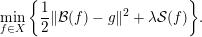 $$\begin{eqnarray}\min _{f\in X}\bigg\{\frac{1}{2}\Vert {\mathcal{B}}(f)-g\Vert ^{2}+\unicode[STIX]{x1D706}{\mathcal{S}}(f)\bigg\}.\end{eqnarray}$$
This can be seen by considering networks similar to the unrolled schemes (see Section 4.9.2); that is, we consider a fully connected feed-forward network with
 $N$
layers. We impose the further restriction that (i) the non-linearity (activation function) is identical to a proximal mapping
$N$
layers. We impose the further restriction that (i) the non-linearity (activation function) is identical to a proximal mapping
 $\operatorname{prox}_{\unicode[STIX]{x1D706}{\mathcal{S}}}$
with respect to a convex functional
$\operatorname{prox}_{\unicode[STIX]{x1D706}{\mathcal{S}}}$
with respect to a convex functional
 ${\mathcal{S}}:X\rightarrow \mathbb{R}$
, (ii) the affine linear mapping between layers allows the decomposition
${\mathcal{S}}:X\rightarrow \mathbb{R}$
, (ii) the affine linear mapping between layers allows the decomposition
 $\text{id}-{\mathcal{W}}=\unicode[STIX]{x1D706}{\mathcal{B}}^{\ast }\circ {\mathcal{B}}$
for some linear operator
$\text{id}-{\mathcal{W}}=\unicode[STIX]{x1D706}{\mathcal{B}}^{\ast }\circ {\mathcal{B}}$
for some linear operator
 ${\mathcal{B}}:X\rightarrow Y$
, and (iii) the bias term is fixed as
${\mathcal{B}}:X\rightarrow Y$
, and (iii) the bias term is fixed as
 $b=\unicode[STIX]{x1D706}{\mathcal{B}}^{\ast }g$
.
$b=\unicode[STIX]{x1D706}{\mathcal{B}}^{\ast }g$
.
As described in Section 4.9.2, the output of a network using this architecture is equivalent to the
 $N$
th iterate of an ISTA scheme for approximating a minimizer of (4.52). With
$N$
th iterate of an ISTA scheme for approximating a minimizer of (4.52). With
 ${\mathcal{W}}=\text{id}-\unicode[STIX]{x1D706}{\mathcal{B}}^{\ast }\circ {\mathcal{B}}$
, the network
${\mathcal{W}}=\text{id}-\unicode[STIX]{x1D706}{\mathcal{B}}^{\ast }\circ {\mathcal{B}}$
, the network
 $\unicode[STIX]{x1D6F9}_{{\mathcal{W}}}^{\dagger }(\unicode[STIX]{x1D709}_{0})$
is given by the unrolled ISTA scheme (Section 4.9.1)
$\unicode[STIX]{x1D6F9}_{{\mathcal{W}}}^{\dagger }(\unicode[STIX]{x1D709}_{0})$
is given by the unrolled ISTA scheme (Section 4.9.1)
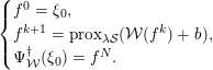 $$\begin{eqnarray}\left\{\begin{array}{@{}ll@{}}f^{0}=\unicode[STIX]{x1D709}_{0},\quad & \\ f^{k+1}=\operatorname{prox}_{\unicode[STIX]{x1D706}{\mathcal{S}}}({\mathcal{W}}(f^{k})+b),\quad & \\ \unicode[STIX]{x1D6F9}_{{\mathcal{W}}}^{\dagger }(\unicode[STIX]{x1D709}_{0})=f^{N}.\quad & \end{array}\right.\end{eqnarray}$$
Such ISTA schemes converge as
 $N\rightarrow \infty$
for rather arbitrary starting points; hence, as pointed out above, the particular choice of
$N\rightarrow \infty$
for rather arbitrary starting points; hence, as pointed out above, the particular choice of
 $\unicode[STIX]{x1D709}_{0}$
in (4.50) is indeed of minor importance.
$\unicode[STIX]{x1D709}_{0}$
in (4.50) is indeed of minor importance.
The starting point for a more in-depth mathematical analysis is the assumption that the above unrolled ISTA scheme has fully converged, that is,
Using this characterization of
 $\hat{f}$
, we define the analytic deep prior as the network, which is obtained by a gradient descent method with respect to
$\hat{f}$
, we define the analytic deep prior as the network, which is obtained by a gradient descent method with respect to
 ${\mathcal{B}}$
for
${\mathcal{B}}$
for
 $$\begin{eqnarray}{\mathcal{L}}({\mathcal{B}},g)=\frac{1}{2}\Vert {\mathcal{A}}(\hat{f})-g\Vert ^{2}.\end{eqnarray}$$
The resulting deep prior network has
 $\operatorname{prox}_{\unicode[STIX]{x1D706}{\mathcal{S}}}$
as activation function, and the linear map
$\operatorname{prox}_{\unicode[STIX]{x1D706}{\mathcal{S}}}$
as activation function, and the linear map
 ${\mathcal{W}}$
and its bias
${\mathcal{W}}$
and its bias
 $b$
are as described in (ii) and (iii). This allows us to obtain an explicit description of the gradient descent for
$b$
are as described in (ii) and (iii). This allows us to obtain an explicit description of the gradient descent for
 ${\mathcal{B}}$
, which in turn leads to an iteration of functionals
${\mathcal{B}}$
, which in turn leads to an iteration of functionals
 ${\mathcal{J}}_{{\mathcal{B}}}$
.
${\mathcal{J}}_{{\mathcal{B}}}$
.
Below, we provide this derivation for a toy example that nevertheless highlights the differences between a classical Tikhonov minimizer and the solution of the DIP approach.
Simple example.
We here examine analytic deep priors for linear inverse problems, i.e.
 ${\mathcal{A}}:X\rightarrow Y$
is linear, and compare them to classical Tikhonov regularization with
${\mathcal{A}}:X\rightarrow Y$
is linear, and compare them to classical Tikhonov regularization with
 ${\mathcal{S}}(f)=\frac{1}{2}\Vert f\Vert ^{2}$
. Let
${\mathcal{S}}(f)=\frac{1}{2}\Vert f\Vert ^{2}$
. Let
 $f_{\unicode[STIX]{x1D706}}\in X$
denote the solution obtained with the classical Tikhonov regularization, which by (2.11) can be expressed as
$f_{\unicode[STIX]{x1D706}}\in X$
denote the solution obtained with the classical Tikhonov regularization, which by (2.11) can be expressed as
 $$\begin{eqnarray}f_{\unicode[STIX]{x1D706}}=({\mathcal{A}}^{\ast }\circ {\mathcal{A}}+\unicode[STIX]{x1D706}\text{id})^{-1}\circ {\mathcal{A}}^{\ast }(g).\end{eqnarray}$$
This is equivalent to the solution obtained by the analytic deep prior approach, with
 ${\mathcal{B}}={\mathcal{A}}$
without any iteration. Now, take
${\mathcal{B}}={\mathcal{A}}$
without any iteration. Now, take
 ${\mathcal{B}}={\mathcal{A}}$
as a starting point for computing a gradient descent with respect to
${\mathcal{B}}={\mathcal{A}}$
as a starting point for computing a gradient descent with respect to
 ${\mathcal{B}}$
using the DIP approach, and compare the resulting
${\mathcal{B}}$
using the DIP approach, and compare the resulting
 $\hat{f}$
with
$\hat{f}$
with
 $f_{\unicode[STIX]{x1D706}}$
.
$f_{\unicode[STIX]{x1D706}}$
.
The proximal mapping for the functional
 $R$
above is given by
$R$
above is given by
 $$\begin{eqnarray}\operatorname{prox}_{\unicode[STIX]{x1D706}{\mathcal{S}}}(z)=\frac{1}{1+\unicode[STIX]{x1D706}}z.\end{eqnarray}$$
A rather lengthy calculation (see Dittmer, Kluth, Maass and Baguer Reference Dittmer, Kluth, Maass and Baguer2018) yields an explicit formula for the derivative of
 $F$
with respect to
$F$
with respect to
 ${\mathcal{B}}$
in the iteration
${\mathcal{B}}$
in the iteration
 $$\begin{eqnarray}{\mathcal{B}}^{k+1}={\mathcal{B}}^{k}-\unicode[STIX]{x1D702}\unicode[STIX]{x2202}F({\mathcal{B}}^{k}).\end{eqnarray}$$
The expression stated there can be made explicit for special settings. For illustration we assume the rather unrealistic case that
 $f^{+}=h$
, where
$f^{+}=h$
, where
 $h\in X$
is a singular function for
$h\in X$
is a singular function for
 ${\mathcal{A}}$
with singular value
${\mathcal{A}}$
with singular value
 $\unicode[STIX]{x1D70E}$
. The dual singular function is denoted by
$\unicode[STIX]{x1D70E}$
. The dual singular function is denoted by
 $v\in Y$
, i.e.
$v\in Y$
, i.e.
 ${\mathcal{A}}h=\unicode[STIX]{x1D70E}v$
and
${\mathcal{A}}h=\unicode[STIX]{x1D70E}v$
and
 ${\mathcal{A}}^{\ast }v=\unicode[STIX]{x1D70E}h$
, and we further assume that the measurement noise in
${\mathcal{A}}^{\ast }v=\unicode[STIX]{x1D70E}h$
, and we further assume that the measurement noise in
 $g$
is in the direction of this singular function, i.e.
$g$
is in the direction of this singular function, i.e.
 $g=(\unicode[STIX]{x1D70E}+\unicode[STIX]{x1D6FF})v$
. In this case, the problem is indeed restricted to the span of
$g=(\unicode[STIX]{x1D70E}+\unicode[STIX]{x1D6FF})v$
. In this case, the problem is indeed restricted to the span of
 $h$
and the span of
$h$
and the span of
 $v$
, respectively. The iterates
$v$
, respectively. The iterates
 ${\mathcal{B}}^{k}$
only change the singular value
${\mathcal{B}}^{k}$
only change the singular value
 $\unicode[STIX]{x1D6FD}_{k}$
of
$\unicode[STIX]{x1D6FD}_{k}$
of
 $h$
, that is,
$h$
, that is,
 $$\begin{eqnarray}{\mathcal{B}}^{k+1}={\mathcal{B}}^{k}-c_{k}\langle \,\cdot \,,h\rangle v,\end{eqnarray}$$
with a suitable
 $c_{k}=c(\unicode[STIX]{x1D706},\unicode[STIX]{x1D6FF},\unicode[STIX]{x1D70E},\unicode[STIX]{x1D702})$
.
$c_{k}=c(\unicode[STIX]{x1D706},\unicode[STIX]{x1D6FF},\unicode[STIX]{x1D70E},\unicode[STIX]{x1D702})$
.
Deep inverse priors for the integration operator.
We now illustrate the use of deep inverse prior approaches for solving an inverse problem with the integration operator
 ${\mathcal{A}}:L^{2}([0,1])\rightarrow L^{2}([0,1])$
, defined by
${\mathcal{A}}:L^{2}([0,1])\rightarrow L^{2}([0,1])$
, defined by
 $$\begin{eqnarray}{\mathcal{A}}(f)(t)=\int _{0}^{t}f(s)\text{d}s.\end{eqnarray}$$
Here
 ${\mathcal{A}}$
is linear and compact, hence the task of evaluating its inverse is an ill-posed inverse problem.
${\mathcal{A}}$
is linear and compact, hence the task of evaluating its inverse is an ill-posed inverse problem.
Discretizing this operator with
 $n=100$
yields a matrix
$n=100$
yields a matrix
 $\mathbf{\mathsf{A}}_{n}\in \mathbb{R}^{n\times n}$
, which has
$\mathbf{\mathsf{A}}_{n}\in \mathbb{R}^{n\times n}$
, which has
 $h/2$
on the main diagonal,
$h/2$
on the main diagonal,
 $h$
everywhere under the main diagonal and
$h$
everywhere under the main diagonal and
 $0$
above (here
$0$
above (here
 $h=1/n$
). We choose
$h=1/n$
). We choose
 $f_{\text{true}}$
to be one of the singular vectors of
$f_{\text{true}}$
to be one of the singular vectors of
 $\mathbf{\mathsf{A}}$
and determine noisy data
$\mathbf{\mathsf{A}}$
and determine noisy data
 $g=\mathbf{\mathsf{A}}_{n}f_{\text{true}}+e$
with
$g=\mathbf{\mathsf{A}}_{n}f_{\text{true}}+e$
with
 $e\sim {\mathcal{N}}(0,\unicode[STIX]{x1D70E}^{2})$
, where
$e\sim {\mathcal{N}}(0,\unicode[STIX]{x1D70E}^{2})$
, where
 $\unicode[STIX]{x1D70E}^{2}$
is chosen as
$\unicode[STIX]{x1D70E}^{2}$
is chosen as
 $10\%$
of the largest coefficient of
$10\%$
of the largest coefficient of
 $g$
; see Figure 4.2.
$g$
; see Figure 4.2.
Example of
 $g$
for
$g$
for
 $f_{\text{true}}=u_{5}$
and
$f_{\text{true}}=u_{5}$
and
 $10\%$
of noise.
$10\%$
of noise.

Figure 4.3 shows some reconstruction results with
 $N=10$
layers. The first plot contains the true solution
$N=10$
layers. The first plot contains the true solution
 $f_{\text{true}}$
, the standard Tikhonov solution
$f_{\text{true}}$
, the standard Tikhonov solution
 $f_{\unicode[STIX]{x1D706}}$
, and the reconstruction obtained with the analytic deep inverse approach
$f_{\unicode[STIX]{x1D706}}$
, and the reconstruction obtained with the analytic deep inverse approach
 $f(\mathbf{\mathsf{B}}_{\text{opt}})$
after
$f(\mathbf{\mathsf{B}}_{\text{opt}})$
after
 $2000$
iterations for updating
$2000$
iterations for updating
 $\mathbf{\mathsf{B}}$
. For both choices of
$\mathbf{\mathsf{B}}$
. For both choices of
 $\unicode[STIX]{x1D706}$
the training of
$\unicode[STIX]{x1D706}$
the training of
 $\mathbf{\mathsf{B}}$
converges to a matrix
$\mathbf{\mathsf{B}}$
converges to a matrix
 $\mathbf{\mathsf{B}}_{\text{opt}}$
, such that
$\mathbf{\mathsf{B}}_{\text{opt}}$
, such that
 $f(\mathbf{\mathsf{B}}_{\text{opt}})$
has a smaller true error than
$f(\mathbf{\mathsf{B}}_{\text{opt}})$
has a smaller true error than
 $f_{\unicode[STIX]{x1D706}}$
. As can be observed in the last plot, the resulting matrix
$f_{\unicode[STIX]{x1D706}}$
. As can be observed in the last plot, the resulting matrix
 $\mathbf{\mathsf{B}}_{\text{opt}}$
contains some patterns that reflect what was predicted by the analytic deep prior.
$\mathbf{\mathsf{B}}_{\text{opt}}$
contains some patterns that reflect what was predicted by the analytic deep prior.
Comparison of Tikhonov reconstructions and results obtained with DIP. Reconstructions are shown for different fixed values of
 $\unicode[STIX]{x1D706}$
. The network was trained with the standard gradient descent method and a learning rate of
$\unicode[STIX]{x1D706}$
. The network was trained with the standard gradient descent method and a learning rate of
 $0.05$
. In (a)
$0.05$
. In (a)
 $500$
epochs were used whereas in (b)
$500$
epochs were used whereas in (b)
 $2000$
were used.
$2000$
were used.
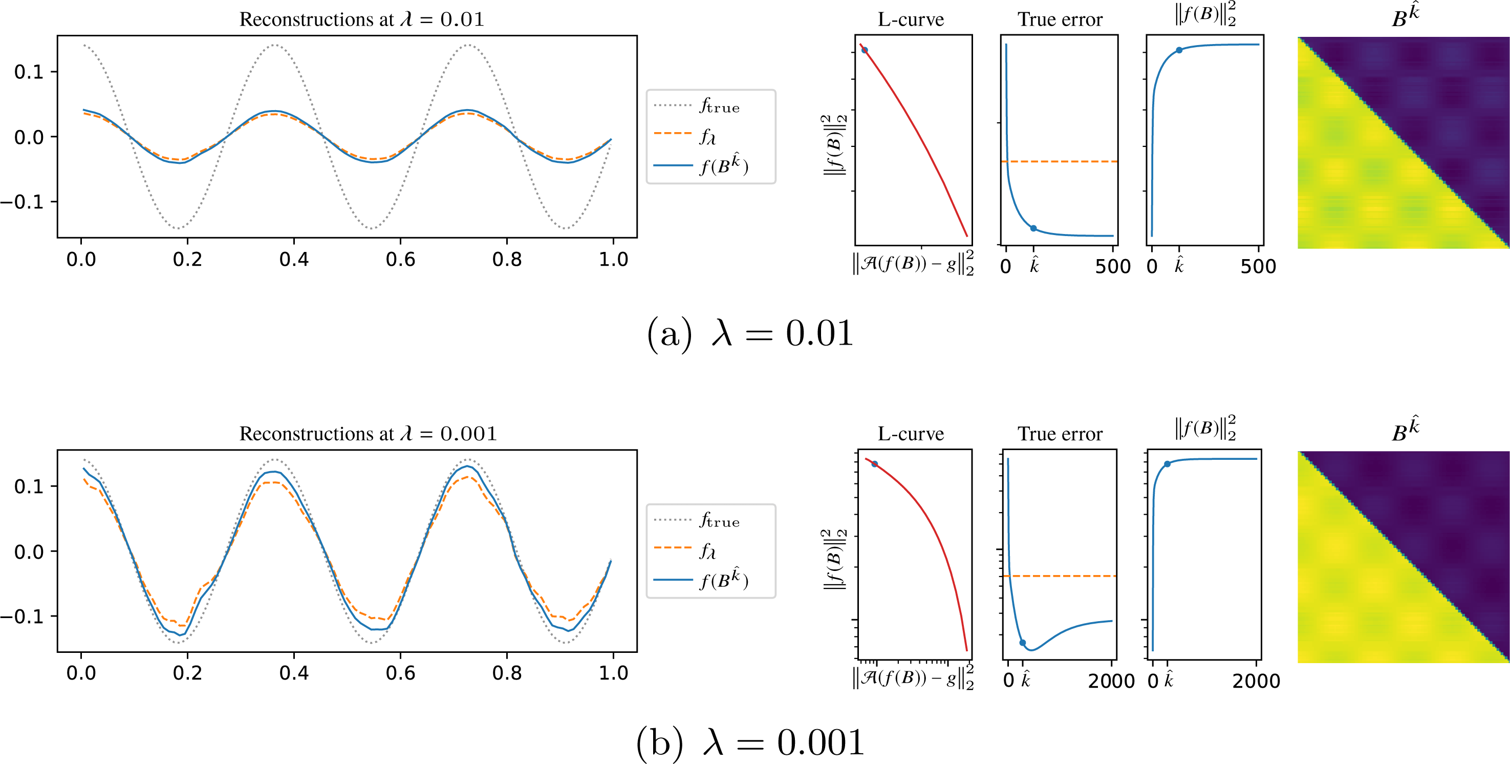
Reconstructions with an adaptive
 $\unicode[STIX]{x1D706}$
for different starting values
$\unicode[STIX]{x1D706}$
for different starting values
 $\unicode[STIX]{x1D706}_{0}$
. The networks were trained with gradient descent using
$\unicode[STIX]{x1D706}_{0}$
. The networks were trained with gradient descent using
 $0.1$
as learning rate. In all cases
$0.1$
as learning rate. In all cases
 $3000$
epochs were used.
$3000$
epochs were used.
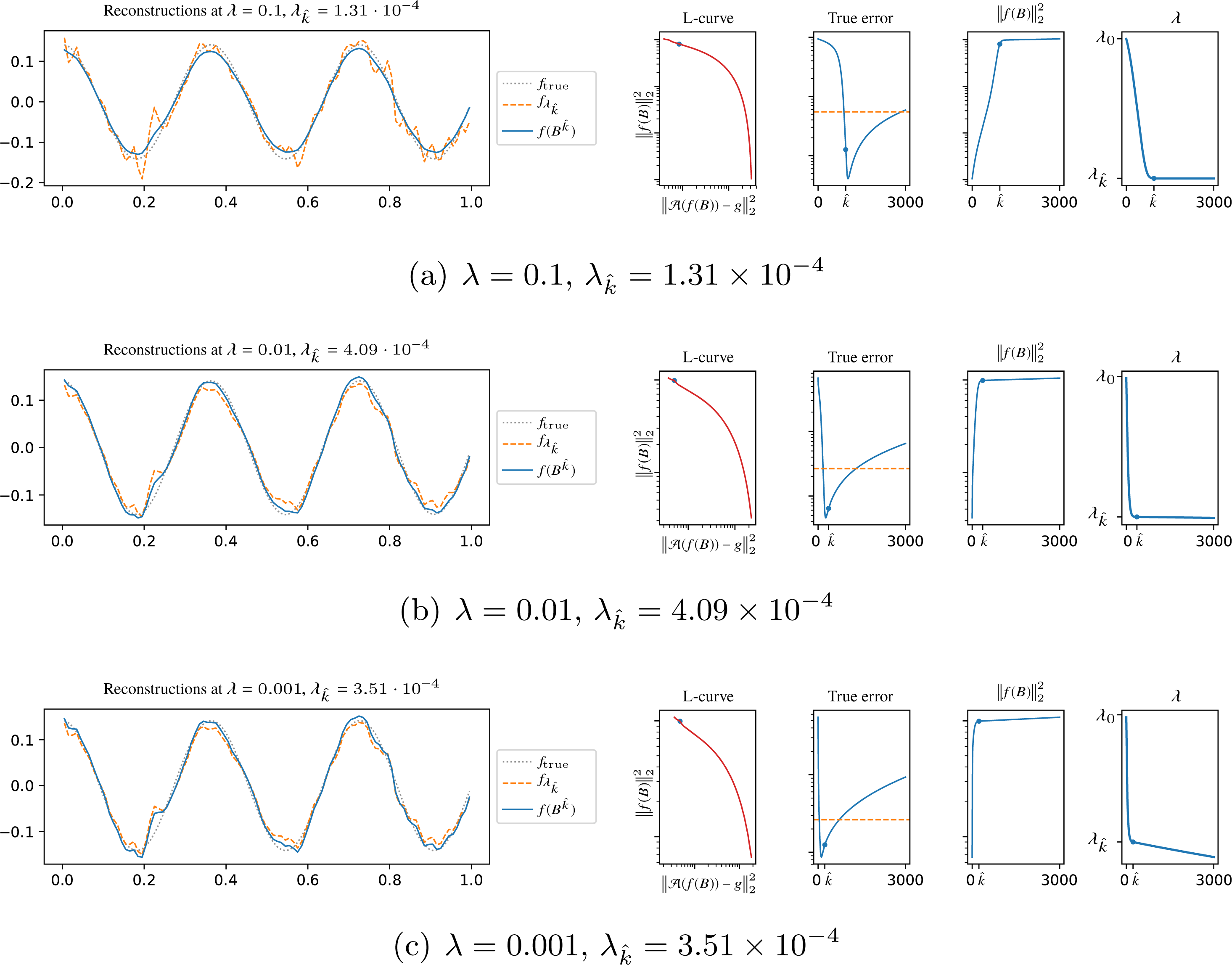
So far, the regularization parameter
 $\unicode[STIX]{x1D706}$
has been assumed to be fixed. In a real application one needs to choose it via a technique such as the L-curve (Hansen Reference Hansen1992) or the discrepancy principle (4.1) in Section 4.1. However, they usually involve finding reconstructions for many different values of
$\unicode[STIX]{x1D706}$
has been assumed to be fixed. In a real application one needs to choose it via a technique such as the L-curve (Hansen Reference Hansen1992) or the discrepancy principle (4.1) in Section 4.1. However, they usually involve finding reconstructions for many different values of
 $\unicode[STIX]{x1D706}$
. In our case, that would mean retraining the network each time, which would lead to a really high computational cost. This motivates an adaptive choice of
$\unicode[STIX]{x1D706}$
. In our case, that would mean retraining the network each time, which would lead to a really high computational cost. This motivates an adaptive choice of
 $\unicode[STIX]{x1D706}$
during the training, which could be achieved by letting
$\unicode[STIX]{x1D706}$
during the training, which could be achieved by letting
 $\unicode[STIX]{x1D706}$
also be a trainable weight of the network. The results for the same example and different starting values
$\unicode[STIX]{x1D706}$
also be a trainable weight of the network. The results for the same example and different starting values
 $\unicode[STIX]{x1D706}_{0}$
are shown in Figure 4.4.
$\unicode[STIX]{x1D706}_{0}$
are shown in Figure 4.4.
5 Learning in statistical regularization
The focus here is on various approaches for combining techniques from deep learning with Bayesian inversion and we begin by recapitulating the statistical setting in Section 3.1.2.
To recapitulate, we assume there exists a
 $(X\times Y)$
-valued random variable
$(X\times Y)$
-valued random variable
 $(\unicode[STIX]{x1D557},\unicode[STIX]{x1D558})\sim \unicode[STIX]{x1D707}$
that generates model parameters with associated data. The aim is to compute various estimators from the posterior
$(\unicode[STIX]{x1D557},\unicode[STIX]{x1D558})\sim \unicode[STIX]{x1D707}$
that generates model parameters with associated data. The aim is to compute various estimators from the posterior
 $\unicode[STIX]{x1D6F1}_{\text{post}}^{g}$
where
$\unicode[STIX]{x1D6F1}_{\text{post}}^{g}$
where
 $g\in Y$
is single sample of
$g\in Y$
is single sample of
 $(\unicode[STIX]{x1D558}\mid \unicode[STIX]{x1D557}=f_{\text{true}})$
with
$(\unicode[STIX]{x1D558}\mid \unicode[STIX]{x1D557}=f_{\text{true}})$
with
 $f_{\text{true}}\in X$
unknown. The data likelihood
$f_{\text{true}}\in X$
unknown. The data likelihood
 $\unicode[STIX]{x1D6F1}_{\text{data}}^{f}$
, which is the distribution of
$\unicode[STIX]{x1D6F1}_{\text{data}}^{f}$
, which is the distribution of
 $(\unicode[STIX]{x1D558}\mid \unicode[STIX]{x1D557}=f)$
, is here known for any
$(\unicode[STIX]{x1D558}\mid \unicode[STIX]{x1D557}=f)$
, is here known for any
 $f\in X$
via (3.3), that is,
$f\in X$
via (3.3), that is,
 $$\begin{eqnarray}\unicode[STIX]{x1D558}={\mathcal{A}}(\unicode[STIX]{x1D557})+\unicode[STIX]{x1D556},\end{eqnarray}$$
with
 $\unicode[STIX]{x1D556}\sim \unicode[STIX]{x1D6F1}_{\text{noise}}$
independent of
$\unicode[STIX]{x1D556}\sim \unicode[STIX]{x1D6F1}_{\text{noise}}$
independent of
 $\unicode[STIX]{x1D557}$
.
$\unicode[STIX]{x1D557}$
.
Ideally one would like to recover the entire posterior distribution
 $f\mapsto \unicode[STIX]{x1D6F1}_{\text{post}}^{g}$
for the measured data
$f\mapsto \unicode[STIX]{x1D6F1}_{\text{post}}^{g}$
for the measured data
 $g$
. However, this is very challenging (Section 3.5), so many approaches settle for computing a selected estimator (Section 5.1). Alternatively, one may use deep neural nets to sample from the posterior, as surveyed in Section 5.2.
$g$
. However, this is very challenging (Section 3.5), so many approaches settle for computing a selected estimator (Section 5.1). Alternatively, one may use deep neural nets to sample from the posterior, as surveyed in Section 5.2.
5.1 Learning an estimator
As outlined in Section 3.3, any reconstruction operator that can be represented by a deterministic measurable map
 ${\mathcal{R}}:Y\rightarrow X$
formally corresponds to a point estimator (also called a non-randomized decision rule). One can now use techniques from deep learning in computing such estimators.
${\mathcal{R}}:Y\rightarrow X$
formally corresponds to a point estimator (also called a non-randomized decision rule). One can now use techniques from deep learning in computing such estimators.
5.1.1 Overview
There are various ways of combining techniques from deep learning with statistical regularization. The statistical characteristics of training data together with the choice of loss function determines the training problem one seeks to solve during learning. This in turn determines the type of estimator (reconstruction operator) one is approximating.
Supervised learning. The training data are given as samples
 $(f_{i},g_{i})\in X\times Y$
generated by
$(f_{i},g_{i})\in X\times Y$
generated by
 $(\unicode[STIX]{x1D557},\unicode[STIX]{x1D558})\sim \unicode[STIX]{x1D707}$
. One can then approximate the Bayes estimator, that is, we seek
$(\unicode[STIX]{x1D557},\unicode[STIX]{x1D558})\sim \unicode[STIX]{x1D707}$
. One can then approximate the Bayes estimator, that is, we seek
 ${\mathcal{R}}_{\widehat{\unicode[STIX]{x1D703}}}:Y\rightarrow X$
, where
${\mathcal{R}}_{\widehat{\unicode[STIX]{x1D703}}}:Y\rightarrow X$
, where
 $\widehat{\unicode[STIX]{x1D703}}$
solves
$\widehat{\unicode[STIX]{x1D703}}$
solves
The actual training involves replacing the joint law
 $\unicode[STIX]{x1D707}$
with its empirical counterpart induced by the supervised training data. Examples of methods that build on the above are surveyed in Section 5.1.2.
$\unicode[STIX]{x1D707}$
with its empirical counterpart induced by the supervised training data. Examples of methods that build on the above are surveyed in Section 5.1.2.
Learned prior. The training data
 $f_{i}\in X$
are samples generated by a
$f_{i}\in X$
are samples generated by a
 $\unicode[STIX]{x1D707}_{\unicode[STIX]{x1D557}}$
-distributed random variable, where
$\unicode[STIX]{x1D707}_{\unicode[STIX]{x1D557}}$
-distributed random variable, where
 $\unicode[STIX]{x1D707}_{\unicode[STIX]{x1D557}}\in \mathscr{P}_{X}$
is the
$\unicode[STIX]{x1D707}_{\unicode[STIX]{x1D557}}\in \mathscr{P}_{X}$
is the
 $\unicode[STIX]{x1D557}$
-marginal of
$\unicode[STIX]{x1D557}$
-marginal of
 $\unicode[STIX]{x1D707}$
. One can then learn the negative log prior density in a MAP estimator, that is,
$\unicode[STIX]{x1D707}$
. One can then learn the negative log prior density in a MAP estimator, that is,
 ${\mathcal{R}}_{\widehat{\unicode[STIX]{x1D703}}}:Y\rightarrow X$
is given by
${\mathcal{R}}_{\widehat{\unicode[STIX]{x1D703}}}:Y\rightarrow X$
is given by
Here
 $\unicode[STIX]{x1D70B}_{\text{data}}(\,\cdot \,\mid f)$
is the density for the data likelihood
$\unicode[STIX]{x1D70B}_{\text{data}}(\,\cdot \,\mid f)$
is the density for the data likelihood
 $\unicode[STIX]{x1D6F1}_{\text{data}}^{f}\in \mathscr{P}_{Y}$
and
$\unicode[STIX]{x1D6F1}_{\text{data}}^{f}\in \mathscr{P}_{Y}$
and
 $\widehat{\unicode[STIX]{x1D703}}$
is learned such that
$\widehat{\unicode[STIX]{x1D703}}$
is learned such that
 ${\mathcal{S}}_{\widehat{\unicode[STIX]{x1D703}}}(f)\approx -\log (\unicode[STIX]{x1D70B}_{\unicode[STIX]{x1D557}}(f))$
, with
${\mathcal{S}}_{\widehat{\unicode[STIX]{x1D703}}}(f)\approx -\log (\unicode[STIX]{x1D70B}_{\unicode[STIX]{x1D557}}(f))$
, with
 $\unicode[STIX]{x1D70B}_{\unicode[STIX]{x1D557}}$
denoting the density for
$\unicode[STIX]{x1D70B}_{\unicode[STIX]{x1D557}}$
denoting the density for
 $\unicode[STIX]{x1D707}_{\unicode[STIX]{x1D557}}\in \mathscr{P}_{X}$
, which is the
$\unicode[STIX]{x1D707}_{\unicode[STIX]{x1D557}}\in \mathscr{P}_{X}$
, which is the
 $\unicode[STIX]{x1D557}$
-marginal of
$\unicode[STIX]{x1D557}$
-marginal of
 $\unicode[STIX]{x1D707}$
. The actual training involves replacing
$\unicode[STIX]{x1D707}$
. The actual training involves replacing
 $\unicode[STIX]{x1D707}_{\unicode[STIX]{x1D557}}$
with its empirical counterpart induced by the training data. Examples of methods that build on the above are surveyed in Section 4.7.
$\unicode[STIX]{x1D707}_{\unicode[STIX]{x1D557}}$
with its empirical counterpart induced by the training data. Examples of methods that build on the above are surveyed in Section 4.7.
Unsupervised learning. The training data
 $\unicode[STIX]{x1D558}_{i}\in Y$
are samples generated by a
$\unicode[STIX]{x1D558}_{i}\in Y$
are samples generated by a
 $\unicode[STIX]{x1D707}_{\unicode[STIX]{x1D558}}$
-distributed random variable where
$\unicode[STIX]{x1D707}_{\unicode[STIX]{x1D558}}$
-distributed random variable where
 $\unicode[STIX]{x1D707}_{\unicode[STIX]{x1D558}}\in \mathscr{P}_{Y}$
is the
$\unicode[STIX]{x1D707}_{\unicode[STIX]{x1D558}}\in \mathscr{P}_{Y}$
is the
 $\unicode[STIX]{x1D558}$
-marginal of
$\unicode[STIX]{x1D558}$
-marginal of
 $\unicode[STIX]{x1D707}$
. It is not possible to learn a prior in a MAP estimator from such training data, but one can improve upon the computational feasibility for evaluating a given MAP estimator. We do that by considering
$\unicode[STIX]{x1D707}$
. It is not possible to learn a prior in a MAP estimator from such training data, but one can improve upon the computational feasibility for evaluating a given MAP estimator. We do that by considering
 ${\mathcal{R}}_{\widehat{\unicode[STIX]{x1D703}}}:Y\rightarrow X$
, where
${\mathcal{R}}_{\widehat{\unicode[STIX]{x1D703}}}:Y\rightarrow X$
, where
 $\widehat{\unicode[STIX]{x1D703}}$
solves
$\widehat{\unicode[STIX]{x1D703}}$
solves
In the above, both the density
 $\unicode[STIX]{x1D70B}_{\text{data}}(\,\cdot \,\mid f)$
for the data likelihood
$\unicode[STIX]{x1D70B}_{\text{data}}(\,\cdot \,\mid f)$
for the data likelihood
 $\unicode[STIX]{x1D6F1}_{\text{data}}^{f}\in \mathscr{P}_{Y}$
and the negative log density
$\unicode[STIX]{x1D6F1}_{\text{data}}^{f}\in \mathscr{P}_{Y}$
and the negative log density
 ${\mathcal{S}}_{\unicode[STIX]{x1D706}}:X\rightarrow \mathbb{R}$
of the prior are handcrafted. The actual training involves replacing
${\mathcal{S}}_{\unicode[STIX]{x1D706}}:X\rightarrow \mathbb{R}$
of the prior are handcrafted. The actual training involves replacing
 $\unicode[STIX]{x1D707}_{\unicode[STIX]{x1D558}}\in \mathscr{P}_{Y}$
with its empirical counterpart induced by the training data. In the above,
$\unicode[STIX]{x1D707}_{\unicode[STIX]{x1D558}}\in \mathscr{P}_{Y}$
with its empirical counterpart induced by the training data. In the above,
 $\widehat{\unicode[STIX]{x1D707}}_{\unicode[STIX]{x1D558}}$
is the empirical counterpart of
$\widehat{\unicode[STIX]{x1D707}}_{\unicode[STIX]{x1D558}}$
is the empirical counterpart of
 $\widehat{\unicode[STIX]{x1D707}}_{\unicode[STIX]{x1D558}}$
given by training data,
$\widehat{\unicode[STIX]{x1D707}}_{\unicode[STIX]{x1D558}}$
given by training data,
 ${\mathcal{L}}:Y\times Y\rightarrow \mathbb{R}$
is the negative data log-likelihood, and
${\mathcal{L}}:Y\times Y\rightarrow \mathbb{R}$
is the negative data log-likelihood, and
 ${\mathcal{S}}_{\unicode[STIX]{x1D706}}:X\rightarrow \mathbb{R}$
is the negative log-prior. The latter two are not learned. Examples of methods that build on the above are surveyed in Section 4.9.
${\mathcal{S}}_{\unicode[STIX]{x1D706}}:X\rightarrow \mathbb{R}$
is the negative log-prior. The latter two are not learned. Examples of methods that build on the above are surveyed in Section 4.9.
Semi-supervised learning. The training data
 $\unicode[STIX]{x1D557}_{i}\in X$
and
$\unicode[STIX]{x1D557}_{i}\in X$
and
 $\unicode[STIX]{x1D558}_{i}\in Y$
are semi-supervised, i.e. unpaired samples from the marginal distributions
$\unicode[STIX]{x1D558}_{i}\in Y$
are semi-supervised, i.e. unpaired samples from the marginal distributions
 $\unicode[STIX]{x1D707}_{\unicode[STIX]{x1D557}}$
and
$\unicode[STIX]{x1D707}_{\unicode[STIX]{x1D557}}$
and
 $\unicode[STIX]{x1D707}_{\unicode[STIX]{x1D558}}$
of
$\unicode[STIX]{x1D707}_{\unicode[STIX]{x1D558}}$
of
 $\unicode[STIX]{x1D707}$
, respectively. One can then compute an estimator
$\unicode[STIX]{x1D707}$
, respectively. One can then compute an estimator
 ${\mathcal{R}}_{\widehat{\unicode[STIX]{x1D703}}}:Y\rightarrow X$
, where
${\mathcal{R}}_{\widehat{\unicode[STIX]{x1D703}}}:Y\rightarrow X$
, where
 $\widehat{\unicode[STIX]{x1D703}}$
solves
$\widehat{\unicode[STIX]{x1D703}}$
solves
In the above,
 $\ell _{X}:X\times X\rightarrow \mathbb{R}$
and
$\ell _{X}:X\times X\rightarrow \mathbb{R}$
and
 $\ell _{Y}:Y\times Y\rightarrow \mathbb{R}$
are loss functions on
$\ell _{Y}:Y\times Y\rightarrow \mathbb{R}$
are loss functions on
 $X$
and
$X$
and
 $Y$
, respectively. Next,
$Y$
, respectively. Next,
 $\ell _{\mathscr{P}_{X}}:\mathscr{P}_{X}\times \mathscr{P}_{X}\rightarrow \mathbb{R}$
is a distance notion between probability distributions on
$\ell _{\mathscr{P}_{X}}:\mathscr{P}_{X}\times \mathscr{P}_{X}\rightarrow \mathbb{R}$
is a distance notion between probability distributions on
 $X$
and
$X$
and
 $({\mathcal{R}}_{\unicode[STIX]{x1D703}})_{\#}(\unicode[STIX]{x1D707}_{\unicode[STIX]{x1D558}})\in \mathscr{P}_{X}$
denotes the pushforward of the measure
$({\mathcal{R}}_{\unicode[STIX]{x1D703}})_{\#}(\unicode[STIX]{x1D707}_{\unicode[STIX]{x1D558}})\in \mathscr{P}_{X}$
denotes the pushforward of the measure
 $\unicode[STIX]{x1D707}_{\unicode[STIX]{x1D558}}\in \mathscr{P}_{Y}$
by
$\unicode[STIX]{x1D707}_{\unicode[STIX]{x1D558}}\in \mathscr{P}_{Y}$
by
 ${\mathcal{R}}_{\unicode[STIX]{x1D703}}:Y\rightarrow X$
. It is common to evaluate
${\mathcal{R}}_{\unicode[STIX]{x1D703}}:Y\rightarrow X$
. It is common to evaluate
 $\ell _{\mathscr{P}_{X}}$
using techniques from GANs, which introduce a separate deep neural network (discriminator/critic). Finally, the parameter
$\ell _{\mathscr{P}_{X}}$
using techniques from GANs, which introduce a separate deep neural network (discriminator/critic). Finally, the parameter
 $\unicode[STIX]{x1D706}$
controls the balance between the distributional consistency, noise suppression and data consistency. One can also consider further variants of the above, for example when there is access to a large sample of unpaired data combined with a small amount of paired data, or when parts of the probability distributions involved are known.
$\unicode[STIX]{x1D706}$
controls the balance between the distributional consistency, noise suppression and data consistency. One can also consider further variants of the above, for example when there is access to a large sample of unpaired data combined with a small amount of paired data, or when parts of the probability distributions involved are known.
The choice of neural network architecture for the reconstruction operator
 ${\mathcal{R}}_{\widehat{\unicode[STIX]{x1D703}}}:Y\rightarrow X$
is formally independent of the choice of loss function and the set-up of the training problem. The choice does, however, impact the trainability of the learning, especially when there is little training data. In such cases, it is important to make use of all the information. In inverse problems one has explicit knowledge about how data are generated that comes in the form of a forward operator, or one might have an expression for the entire data likelihood. Architectures that embed such explicit knowledge, e.g. the forward operator and the adjoint of its derivative, perform better when there is little training data. They also have better generalization properties, and against adversarial attacks (Chakraborty et al.
Reference Chakraborty, Alam, Dey, Chattopadhyay and Mukhopadhyay2018, Akhtar and Mian Reference Akhtar and Mian2018) they are more difficult to design since a successful attack needs to be consistent with how data are generated. Architectures that account for such information can be defined by unrolling (Section 4.9.4).
${\mathcal{R}}_{\widehat{\unicode[STIX]{x1D703}}}:Y\rightarrow X$
is formally independent of the choice of loss function and the set-up of the training problem. The choice does, however, impact the trainability of the learning, especially when there is little training data. In such cases, it is important to make use of all the information. In inverse problems one has explicit knowledge about how data are generated that comes in the form of a forward operator, or one might have an expression for the entire data likelihood. Architectures that embed such explicit knowledge, e.g. the forward operator and the adjoint of its derivative, perform better when there is little training data. They also have better generalization properties, and against adversarial attacks (Chakraborty et al.
Reference Chakraborty, Alam, Dey, Chattopadhyay and Mukhopadhyay2018, Akhtar and Mian Reference Akhtar and Mian2018) they are more difficult to design since a successful attack needs to be consistent with how data are generated. Architectures that account for such information can be defined by unrolling (Section 4.9.4).
The remaining sections survey various approaches from the literature in computing the above estimators.
5.1.2 Deep direct Bayes estimation
The aim is to compute a Bayes estimator, which by the definition given in (3.14) amounts to finding a reconstruction operator
 ${\mathcal{R}}_{\unicode[STIX]{x1D707}}:Y\rightarrow X$
that solves
${\mathcal{R}}_{\unicode[STIX]{x1D707}}:Y\rightarrow X$
that solves
where
 $\ell _{X}:X\times X\rightarrow \mathbb{R}$
is a fixed loss function. The data likelihood is often known, and by the law of total probability we have
$\ell _{X}:X\times X\rightarrow \mathbb{R}$
is a fixed loss function. The data likelihood is often known, and by the law of total probability we have
so the joint law
 $\unicode[STIX]{x1D707}$
is known as soon as a prior has been selected.
$\unicode[STIX]{x1D707}$
is known as soon as a prior has been selected.
As already mentioned (Section 3.5.1), selecting an appropriate prior that reflects the probability distribution of natural model parameters is very challenging, and current hand-crafted choices (Section 3.4) do not capture the full extent of the available a priori information about the true unknown model parameter
 $f_{\text{true}}\in X$
. Next, the expression in (5.4) involves taking an expectation over
$f_{\text{true}}\in X$
. Next, the expression in (5.4) involves taking an expectation over
 $X\times Y$
as well as an optimization over all possible non-randomized decision rules. Both these operations easily become computationally overwhelming in large-scale inverse problem, such as those that arise in imaging.
$X\times Y$
as well as an optimization over all possible non-randomized decision rules. Both these operations easily become computationally overwhelming in large-scale inverse problem, such as those that arise in imaging.
These issues can be addressed by using techniques from supervised training. To start with, one can restrict the minimization in (5.4) to a family of reconstruction methods parametrized by a deep neural network architecture
 ${\mathcal{R}}_{\unicode[STIX]{x1D703}}:Y\rightarrow X$
. Next, the unknown joint law
${\mathcal{R}}_{\unicode[STIX]{x1D703}}:Y\rightarrow X$
. Next, the unknown joint law
 $\unicode[STIX]{x1D707}$
can be replaced with its empirical counterpart given by supervised training data
$\unicode[STIX]{x1D707}$
can be replaced with its empirical counterpart given by supervised training data
 $$\begin{eqnarray}\unicode[STIX]{x1D6F4}_{m}:=\{(f_{1},g_{1}),\ldots ,(f_{m},g_{m})\}\subset X\times Y,\end{eqnarray}$$
where
 $(f_{i},g_{i})$
are generated by
$(f_{i},g_{i})$
are generated by
 $(\unicode[STIX]{x1D557},\unicode[STIX]{x1D558})\sim \unicode[STIX]{x1D707}$
. If there is a sufficient amount of such training data, then one can approximate the Bayes estimator in (5.4) by the neural network
$(\unicode[STIX]{x1D557},\unicode[STIX]{x1D558})\sim \unicode[STIX]{x1D707}$
. If there is a sufficient amount of such training data, then one can approximate the Bayes estimator in (5.4) by the neural network
 ${\mathcal{R}}_{\widehat{\unicode[STIX]{x1D703}}}:Y\rightarrow X$
, where the finite-dimensional network parameter
${\mathcal{R}}_{\widehat{\unicode[STIX]{x1D703}}}:Y\rightarrow X$
, where the finite-dimensional network parameter
 $\widehat{\unicode[STIX]{x1D703}}\in \unicode[STIX]{x1D6E9}$
is learned from data by solving the following empirical risk minimization problem:
$\widehat{\unicode[STIX]{x1D703}}\in \unicode[STIX]{x1D6E9}$
is learned from data by solving the following empirical risk minimization problem:
where
 $(f_{i},g_{i})\in \unicode[STIX]{x1D6F4}_{m}$
as in (5.6). Note now that (5.7) does not explicitly require specifying a prior
$(f_{i},g_{i})\in \unicode[STIX]{x1D6F4}_{m}$
as in (5.6). Note now that (5.7) does not explicitly require specifying a prior
 $f\mapsto \unicode[STIX]{x1D6F1}_{\text{prior}}(f)$
or a data likelihood
$f\mapsto \unicode[STIX]{x1D6F1}_{\text{prior}}(f)$
or a data likelihood
 $g\mapsto \unicode[STIX]{x1D6F1}_{\text{data}}^{f}$
that models how data are generated given a model parameter. Information about both of these is implicitly contained in supervised training data
$g\mapsto \unicode[STIX]{x1D6F1}_{\text{data}}^{f}$
that models how data are generated given a model parameter. Information about both of these is implicitly contained in supervised training data
 $\unicode[STIX]{x1D6F4}_{m}\subset X\times Y$
.
$\unicode[STIX]{x1D6F4}_{m}\subset X\times Y$
.
Fully learned Bayes estimation (Section 5.1.3) refers to approaches where one assumes there is enough supervised training data to learn the joint law
 $\unicode[STIX]{x1D707}$
, that is, one disregards the explicit knowledge about the data likelihood. In contrast, learned iterative schemes (Section 5.1.4) include the information about the data likelihood by using an appropriate architecture of
$\unicode[STIX]{x1D707}$
, that is, one disregards the explicit knowledge about the data likelihood. In contrast, learned iterative schemes (Section 5.1.4) include the information about the data likelihood by using an appropriate architecture of
 ${\mathcal{R}}_{\unicode[STIX]{x1D703}}:Y\rightarrow X$
. Learned post-processing methods (Section 5.1.5) offer an alternative way to account for the data likelihood since these methods apply an initial reconstruction operator that maps data to a model parameter. This is actually an estimator different from the above Bayes estimator, but if the loss is the squared
${\mathcal{R}}_{\unicode[STIX]{x1D703}}:Y\rightarrow X$
. Learned post-processing methods (Section 5.1.5) offer an alternative way to account for the data likelihood since these methods apply an initial reconstruction operator that maps data to a model parameter. This is actually an estimator different from the above Bayes estimator, but if the loss is the squared
 $L^{2}$
-norm and the initial reconstruction operator is a linear sufficient statistic, then these estimators coincide in the ‘large-sample’ or ‘small-noise’ limit.
$L^{2}$
-norm and the initial reconstruction operator is a linear sufficient statistic, then these estimators coincide in the ‘large-sample’ or ‘small-noise’ limit.
Regularizing the learning.
The problem in (5.7) is ill-posed in itself, so one should not try to solve it in the formal sense. A wide range of techniques have been developed within supervised learning for implicitly or explicitly regularizing the empirical risk minimization problem in (5.7) as surveyed and categorized by Kukačka, Golkov and Cremers (Reference Kukačka, Golkov and Cremers2017). A key challenge is to handle the non-convexity, and the energy landscape for the objective in (5.7) typically has many local minima: for example, for binary classification there is an exponential number (in terms of network parameters) of distinct local minima (Auer, Herbster and Warmuth Reference Auer, Herbster and Warmuth1996).
Similar to Shai and Shai (Reference Shai and Shai2014, Section 2.1), we define a training algorithm for (5.7) as an operator mapping a probability measure on
 $X\times Y$
to a parameter in
$X\times Y$
to a parameter in
 $\unicode[STIX]{x1D6E9}$
that approximately solves (5.7):
$\unicode[STIX]{x1D6E9}$
that approximately solves (5.7):
 $$\begin{eqnarray}{\mathcal{T}}:\mathscr{P}_{X\times Y}\rightarrow \unicode[STIX]{x1D6E9},\end{eqnarray}$$
where
 ${\mathcal{T}}(\widehat{\unicode[STIX]{x1D707}})\approx \widehat{\unicode[STIX]{x1D703}}$
with
${\mathcal{T}}(\widehat{\unicode[STIX]{x1D707}})\approx \widehat{\unicode[STIX]{x1D703}}$
with
 $\widehat{\unicode[STIX]{x1D703}}\in \unicode[STIX]{x1D6E9}$
denoting a solution to (5.7). Thus, the training algorithm is a method for approximately solving (5.7) given a fixed neural network architecture. This also includes necessary regularization techniques: for example, a common strategy for solving (5.7) is to use some variant of stochastic gradient descent that is cleverly initialized (often at random from a specific distribution) along with techniques to ensure that the value of the objective (training error) decreases sufficiently rapidly. This, combined with early stopping (i.e. not fully solving (5.7)), warm-start, use of mini-batches, adding a regularization term to the objective, and so on, acts as a regularization (Ruder Reference Ruder2016, Kukačka et al.
Reference Kukačka, Golkov and Cremers2017, Bottou, Curtis and Nocedal Reference Bottou, Curtis and Nocedal2018).
$\widehat{\unicode[STIX]{x1D703}}\in \unicode[STIX]{x1D6E9}$
denoting a solution to (5.7). Thus, the training algorithm is a method for approximately solving (5.7) given a fixed neural network architecture. This also includes necessary regularization techniques: for example, a common strategy for solving (5.7) is to use some variant of stochastic gradient descent that is cleverly initialized (often at random from a specific distribution) along with techniques to ensure that the value of the objective (training error) decreases sufficiently rapidly. This, combined with early stopping (i.e. not fully solving (5.7)), warm-start, use of mini-batches, adding a regularization term to the objective, and so on, acts as a regularization (Ruder Reference Ruder2016, Kukačka et al.
Reference Kukačka, Golkov and Cremers2017, Bottou, Curtis and Nocedal Reference Bottou, Curtis and Nocedal2018).
Concerning the model architecture, there is strong empirical evidence that the choice of neural network architecture has an influence on the ill-posedness of (5.7) (Li, Xu, Taylor and Goldstein Reference Li, Xu, Taylor and Goldstein2018c
, Draxler, Veschgini, Salmhofer and Hamprecht Reference Draxler, Veschgini, Salmhofer and Hamprecht2018). Many tasks that are successfully solved by supervised learning rely on (deep) neural networks, which can approximate a wide range of non-linear phenomena (large model capacity) without impairing computability. For this reason we consider deep neural networks to parametrize
 ${\mathcal{R}}_{\unicode[STIX]{x1D703}}:Y\rightarrow X$
. Furthermore, empirical evidence indicates that deep neural network architectures yield a more favourable energy landscape for the objective of (5.7) than shallow ones: for example, most local minima are almost global (Choromanska et al.
Reference Choromanska, Henaff, Mathieu, Arous and LeCun2015, Becker, Zhang and Lee Reference Becker, Zhang and Lee2018). This intricate interplay between the choice of architecture and avoiding getting trapped in ‘bad’ local minima is poorly understood, and it is an active area of research within the machine learning community. Despite the lack of a theory, there is a consensus that an appropriate model architecture not only ensures computational feasibility but also acts as a kind of implicit regularization for (5.7).
${\mathcal{R}}_{\unicode[STIX]{x1D703}}:Y\rightarrow X$
. Furthermore, empirical evidence indicates that deep neural network architectures yield a more favourable energy landscape for the objective of (5.7) than shallow ones: for example, most local minima are almost global (Choromanska et al.
Reference Choromanska, Henaff, Mathieu, Arous and LeCun2015, Becker, Zhang and Lee Reference Becker, Zhang and Lee2018). This intricate interplay between the choice of architecture and avoiding getting trapped in ‘bad’ local minima is poorly understood, and it is an active area of research within the machine learning community. Despite the lack of a theory, there is a consensus that an appropriate model architecture not only ensures computational feasibility but also acts as a kind of implicit regularization for (5.7).
To summarize, a training algorithm
 ${\mathcal{T}}$
as in (5.8) together with a specific model architecture regularizes (5.7), thereby resulting in the following approximation to the Bayes estimator (5.4):
${\mathcal{T}}$
as in (5.8) together with a specific model architecture regularizes (5.7), thereby resulting in the following approximation to the Bayes estimator (5.4):
 $$\begin{eqnarray}{\mathcal{R}}_{{\mathcal{T}}(\widehat{\unicode[STIX]{x1D707}})}:Y\rightarrow X\end{eqnarray}$$
for the empirical measure
 $\widehat{\unicode[STIX]{x1D707}}$
given by
$\widehat{\unicode[STIX]{x1D707}}$
given by
 $\unicode[STIX]{x1D6F4}_{m}\subset X\times Y$
as in (5.6).
$\unicode[STIX]{x1D6F4}_{m}\subset X\times Y$
as in (5.6).
5.1.3 Fully learned Bayes estimation
Here the reconstruction operator
 ${\mathcal{R}}_{\unicode[STIX]{x1D703}}:Y\rightarrow X$
has a generic parametrization given by a deep neural network that does not explicitly account for the data likelihood.
${\mathcal{R}}_{\unicode[STIX]{x1D703}}:Y\rightarrow X$
has a generic parametrization given by a deep neural network that does not explicitly account for the data likelihood.
An obvious difficulty with this approach is that the data space
 $Y$
and model parameter space
$Y$
and model parameter space
 $X$
are mathematically different. Without an explicit mapping from
$X$
are mathematically different. Without an explicit mapping from
 $Y$
to
$Y$
to
 $X$
the action of convolutional layer operators cannot be properly defined. Therefore, fully learned approaches usually involve one or more ‘fully connected layers’ that represent a pseudo-inverse operator
$X$
the action of convolutional layer operators cannot be properly defined. Therefore, fully learned approaches usually involve one or more ‘fully connected layers’ that represent a pseudo-inverse operator
 ${\mathcal{B}}_{\unicode[STIX]{x1D703}_{1}}:Y\rightarrow X$
mapping elements in
${\mathcal{B}}_{\unicode[STIX]{x1D703}_{1}}:Y\rightarrow X$
mapping elements in
 $Y$
to elements in
$Y$
to elements in
 $X$
followed by a conventional neural network for
$X$
followed by a conventional neural network for
 ${\mathcal{F}}_{\unicode[STIX]{x1D703}_{2}}:X\rightarrow X$
, that is, we get
${\mathcal{F}}_{\unicode[STIX]{x1D703}_{2}}:X\rightarrow X$
, that is, we get
 $$\begin{eqnarray}{\mathcal{R}}_{\unicode[STIX]{x1D703}}:={\mathcal{F}}_{\unicode[STIX]{x1D703}_{2}}\circ {\mathcal{B}}_{\unicode[STIX]{x1D703}_{1}}\quad \text{with }\unicode[STIX]{x1D703}=(\unicode[STIX]{x1D703}_{1},\unicode[STIX]{x1D703}_{2}).\end{eqnarray}$$
In the discrete setting, where
 $Y=\mathbb{R}^{n}$
and
$Y=\mathbb{R}^{n}$
and
 $X=\mathbb{R}^{m}$
, the simplest representation for
$X=\mathbb{R}^{m}$
, the simplest representation for
 ${\mathcal{B}}$
is a dense matrix
${\mathcal{B}}$
is a dense matrix
 $\mathbf{\mathsf{B}}\in \mathbb{R}^{m\times n}$
; the inclusion of an activation function makes this a non-linear mapping.
$\mathbf{\mathsf{B}}\in \mathbb{R}^{m\times n}$
; the inclusion of an activation function makes this a non-linear mapping.
Initial examples of fully learned reconstruction in tomographic imaging include Paschalis et al. (Reference Paschalis, Giokaris, Karabarbounis, Loudos, Maintas, Papanicolas, Spanoudaki, Tsoumpas and Stiliaris2004) for SPECT imaging and Argyrou, Maintas, Tsoumpas and Stiliaris (Reference Argyrou, Maintas, Tsoumpas and Stiliaris2012) for transmission tomography. Both papers consider small-scale problems: for example, Paschalis et al. (Reference Paschalis, Giokaris, Karabarbounis, Loudos, Maintas, Papanicolas, Spanoudaki, Tsoumpas and Stiliaris2004) consider recovering
 $27\times 27$
pixel single photon emission computed tomography (SPECT) images, and Argyrou et al. (Reference Argyrou, Maintas, Tsoumpas and Stiliaris2012) consider recovering
$27\times 27$
pixel single photon emission computed tomography (SPECT) images, and Argyrou et al. (Reference Argyrou, Maintas, Tsoumpas and Stiliaris2012) consider recovering
 $64\times 64$
pixel images from tomographic data.
$64\times 64$
pixel images from tomographic data.
A more recent example is the automated transform by manifold approximation (AUTOMAP) method introduced in Zhu et al. (Reference Zhu, Liu, Cauley, Rosen and Rosen2018) as a tool for fully data-driven image reconstruction. Here,
 ${\mathcal{R}}_{\unicode[STIX]{x1D703}}:Y\rightarrow X$
is represented by a feed-forward deep neural network with fully connected layers followed by a sparse convolutional auto-encoder. This is in some sense similar to the Deep Cascade architecture in Schlemper et al. (Reference Schlemper, Caballero, Hajnal, Price and Rueckert2017), as it has one portion of the network for data consistency and the other for super-resolution/refinement of image quality. The encoder from data space to the model parameter space is implemented using three consecutive fully connected networks with
${\mathcal{R}}_{\unicode[STIX]{x1D703}}:Y\rightarrow X$
is represented by a feed-forward deep neural network with fully connected layers followed by a sparse convolutional auto-encoder. This is in some sense similar to the Deep Cascade architecture in Schlemper et al. (Reference Schlemper, Caballero, Hajnal, Price and Rueckert2017), as it has one portion of the network for data consistency and the other for super-resolution/refinement of image quality. The encoder from data space to the model parameter space is implemented using three consecutive fully connected networks with
 $\sinh$
activation functions followed by two CNN layers with ReLU activation. We interpret this as a combination of a pseudo-inverse
$\sinh$
activation functions followed by two CNN layers with ReLU activation. We interpret this as a combination of a pseudo-inverse
 $\{_{\unicode[STIX]{x1D703}_{3}}^{\dagger }:Y\rightarrow X$
with a conventional convolutional auto-encoder:
$\{_{\unicode[STIX]{x1D703}_{3}}^{\dagger }:Y\rightarrow X$
with a conventional convolutional auto-encoder:
 $$\begin{eqnarray}{\mathcal{R}}_{\unicode[STIX]{x1D703}}=\underbrace{\unicode[STIX]{x1D6F9}_{\unicode[STIX]{x1D703}_{1}}^{\dagger }\circ \unicode[STIX]{x1D6F9}_{\unicode[STIX]{x1D703}_{2}}}_{\text{auto-encoder}}\circ \{_{\unicode[STIX]{x1D703}_{3}}^{\dagger }\quad \text{for }\unicode[STIX]{x1D703}=(\unicode[STIX]{x1D703}_{1},\unicode[STIX]{x1D703}_{2}.\unicode[STIX]{x1D703}_{3}).\end{eqnarray}$$
AUTOMAP was used to reconstruct
 $128\times 128$
pixel images from MRI and PET imaging data. The dependence on fully connected layers results in a large number of neural network parameters that have to be trained. Primarily motivated by this difficulty, a further development of AUTOMAP is ETER-net (Oh et al.
Reference Oh, Kim, Chung, Han, Park and Knoll2018), which uses a recurrent neural network architecture in place of the fully connected/convolutional auto-encoder architecture. Also addressing
$128\times 128$
pixel images from MRI and PET imaging data. The dependence on fully connected layers results in a large number of neural network parameters that have to be trained. Primarily motivated by this difficulty, a further development of AUTOMAP is ETER-net (Oh et al.
Reference Oh, Kim, Chung, Han, Park and Knoll2018), which uses a recurrent neural network architecture in place of the fully connected/convolutional auto-encoder architecture. Also addressing
 $128\times 128$
pixel images from MRI, Oh et al. (Reference Oh, Kim, Chung, Han, Park and Knoll2018) found a reduction in required parameters by over 80%. A method similar to AUTOMAP is used by Yoo et al. (Reference Yoo, Sabir, Heo, Kim, Wahab, Choi, Lee, Chae, Kim, Bae, Choi, Cho and Ye2017) to solve the non-linear reconstruction problem in diffuse optical tomography. Here the forward problem is the Lippman–Schwinger equation but only a single fully connected layer is used in the backprojection step. Yoo et al. (Reference Yoo, Sabir, Heo, Kim, Wahab, Choi, Lee, Chae, Kim, Bae, Choi, Cho and Ye2017) exploit the intrinsically ill-posed nature of the forward problem to argue that the mapping induced by the auto-encoder step is low-rank and therefore sets an upper bound on the dimension of the hidden convolution layers.
$128\times 128$
pixel images from MRI, Oh et al. (Reference Oh, Kim, Chung, Han, Park and Knoll2018) found a reduction in required parameters by over 80%. A method similar to AUTOMAP is used by Yoo et al. (Reference Yoo, Sabir, Heo, Kim, Wahab, Choi, Lee, Chae, Kim, Bae, Choi, Cho and Ye2017) to solve the non-linear reconstruction problem in diffuse optical tomography. Here the forward problem is the Lippman–Schwinger equation but only a single fully connected layer is used in the backprojection step. Yoo et al. (Reference Yoo, Sabir, Heo, Kim, Wahab, Choi, Lee, Chae, Kim, Bae, Choi, Cho and Ye2017) exploit the intrinsically ill-posed nature of the forward problem to argue that the mapping induced by the auto-encoder step is low-rank and therefore sets an upper bound on the dimension of the hidden convolution layers.
The advantage of fully learned Bayes estimation lies in its simplicity, since one avoids making use of an explicit forward operator (or data likelihood). On the other hand, any generic approach to reconstruction by deep neural networks requires having connected layers that represent the relation between model parameters and data. For this reason, generic fully learned Bayes estimation will always scale badly: for example, in three-dimensional tomographic reconstruction it is common to have an inverse problem which, when discretized, involves recovering a
 $(512\times 512\times 512\approx 10^{8})$
-dimensional model parameter from data of the same order of magnitude. Hence, a fully learned generic approach would involve learning at least
$(512\times 512\times 512\approx 10^{8})$
-dimensional model parameter from data of the same order of magnitude. Hence, a fully learned generic approach would involve learning at least
 $10^{16}$
weights from supervised data! There have been several attempts to address the above issue by considering neural network architectures that are adapted to specific direct and inverse problems. One example is that of Khoo and Ying (Reference Khoo and Ying2018), who provide a novel neural network architecture (SwitchNet) for solving inverse scattering problems involving the wave equation. By leveraging the inherent low-rank structure of the scattering problems and introducing a novel switching layer with sparse connections, the SwitchNet architecture uses far fewer parameters than a U-Net architecture for such problems. Another example is that of Ardizzone et al. (Reference Ardizzone, Kruse, Wirkert, Rahner, Pellegrini, Klessen, Maier-Hein, Rother and Köthe2018), who propose encoding the forward operator using a invertible neural network, also called a reversible residual network (Gomez, Ren, Urtasun and Grosse Reference Gomez, Ren, Urtasun and Grosse2017). The reconstruction operator is then obtained as the inverse of the invertible neural network for the forward operator. However, it is unclear whether this is a clever approach to problems that are ill-posed, since an inverse of the forward operator is not stable. Another approach is that of Yoo et al. (Reference Yoo, Sabir, Heo, Kim, Wahab, Choi, Lee, Chae, Kim, Bae, Choi, Cho and Ye2017), who apply an AUTOMAP-like architecture for non-linear reconstruction problems in diffuse optical tomography. Here the forward problem is the Lippman–Schwinger equation, but only a single fully connected layer is used in the backprojection step. Yoo et al. (Reference Yoo, Sabir, Heo, Kim, Wahab, Choi, Lee, Chae, Kim, Bae, Choi, Cho and Ye2017) exploit the intrinsically ill-posed nature of the forward problem to argue that the mapping induced by the auto-encoder step is low-rank and therefore sets an upper bound on the dimension of the hidden convolution layers. The above approaches can also to some extent be seen as further refinements of methods in Section 4.2.
$10^{16}$
weights from supervised data! There have been several attempts to address the above issue by considering neural network architectures that are adapted to specific direct and inverse problems. One example is that of Khoo and Ying (Reference Khoo and Ying2018), who provide a novel neural network architecture (SwitchNet) for solving inverse scattering problems involving the wave equation. By leveraging the inherent low-rank structure of the scattering problems and introducing a novel switching layer with sparse connections, the SwitchNet architecture uses far fewer parameters than a U-Net architecture for such problems. Another example is that of Ardizzone et al. (Reference Ardizzone, Kruse, Wirkert, Rahner, Pellegrini, Klessen, Maier-Hein, Rother and Köthe2018), who propose encoding the forward operator using a invertible neural network, also called a reversible residual network (Gomez, Ren, Urtasun and Grosse Reference Gomez, Ren, Urtasun and Grosse2017). The reconstruction operator is then obtained as the inverse of the invertible neural network for the forward operator. However, it is unclear whether this is a clever approach to problems that are ill-posed, since an inverse of the forward operator is not stable. Another approach is that of Yoo et al. (Reference Yoo, Sabir, Heo, Kim, Wahab, Choi, Lee, Chae, Kim, Bae, Choi, Cho and Ye2017), who apply an AUTOMAP-like architecture for non-linear reconstruction problems in diffuse optical tomography. Here the forward problem is the Lippman–Schwinger equation, but only a single fully connected layer is used in the backprojection step. Yoo et al. (Reference Yoo, Sabir, Heo, Kim, Wahab, Choi, Lee, Chae, Kim, Bae, Choi, Cho and Ye2017) exploit the intrinsically ill-posed nature of the forward problem to argue that the mapping induced by the auto-encoder step is low-rank and therefore sets an upper bound on the dimension of the hidden convolution layers. The above approaches can also to some extent be seen as further refinements of methods in Section 4.2.
However, neither of the above efforts address the challenge of finding sufficient supervised training data necessary for the training. Furthermore, any changes to the acquisition protocol or instrumentation may require retraining, making the method impractical. In particular, due to the lack of training data, fully learned Bayes estimation is inapplicable to cases when data are acquired using novel instrumentation. A practical case would be spectral CT, where novel direct counting energy resolving detectors are being developed.
5.1.4 Learned iterative schemes
The idea here is to choose an architecture for
 ${\mathcal{R}}_{\unicode[STIX]{x1D703}}:Y\rightarrow X$
in (5.7) that contains an explicit expression for the data likelihood, which accounts for how a model parameter gives rise to data. This requires us to embed an explicit forward operator
${\mathcal{R}}_{\unicode[STIX]{x1D703}}:Y\rightarrow X$
in (5.7) that contains an explicit expression for the data likelihood, which accounts for how a model parameter gives rise to data. This requires us to embed an explicit forward operator
 ${\mathcal{A}}:X\rightarrow Y$
into the architecture for
${\mathcal{A}}:X\rightarrow Y$
into the architecture for
 ${\mathcal{R}}_{\unicode[STIX]{x1D703}}$
, which is somewhat tricky since
${\mathcal{R}}_{\unicode[STIX]{x1D703}}$
, which is somewhat tricky since
 ${\mathcal{R}}_{\unicode[STIX]{x1D703}}$
and
${\mathcal{R}}_{\unicode[STIX]{x1D703}}$
and
 ${\mathcal{A}}$
are mappings that go in the reverse direction compared to each other.
${\mathcal{A}}$
are mappings that go in the reverse direction compared to each other.
One approach is presented by Mousavi and Baraniuk (Reference Mousavi and Baraniuk2017), who suggest a CNN architecture (DeepInverse) adapted for solving a linear inverse problem. The architecture involves a fully connected layer (that is not learned) to represent the normal operator
 ${\mathcal{A}}^{\ast }\circ {\mathcal{A}}:X\rightarrow X$
followed by convolutional layers as in a regular CNN with ReLU activation, but here one dispenses with the downsampling (max-pooling operation) that is common in a CNN. The usefulness is limited, however, since the normal operator needs to have a certain structure for the sake of computational efficiency, for example when inverting the Fourier transform, which results in a block-circulant matrix.
${\mathcal{A}}^{\ast }\circ {\mathcal{A}}:X\rightarrow X$
followed by convolutional layers as in a regular CNN with ReLU activation, but here one dispenses with the downsampling (max-pooling operation) that is common in a CNN. The usefulness is limited, however, since the normal operator needs to have a certain structure for the sake of computational efficiency, for example when inverting the Fourier transform, which results in a block-circulant matrix.
Another class of methods is that of learned iterative schemes, which include a handcrafted forward operator and the adjoint of its derivative into the architecture by unrolling a suitable iterative scheme (Section 4.9.4). An early variant was presented by Yang, Sun, Li and Xu (Reference Yang, Sun, Li, Xu and Lee2016), who define a learned iterative method based on unrolling an ADMM-type scheme. The network is trained against supervised data using a somewhat unusual asymmetric loss, namely
 $$\begin{eqnarray}\ell _{X}(f,h):=\sqrt{\Vert f-h\Vert _{2}^{2}/\Vert f\Vert _{2}^{2}}.\end{eqnarray}$$
The trained network is used to invert the Fourier transform (MRI image reconstruction). However, the whole approach is unnecessarily complex, and it is now surpassed by learned iterative methods that have a more transparent logic. The survey will therefore focus on these latter variants.
Learned iterative in model parameter space.
In the simplest setting,
 ${\mathcal{R}}_{\unicode[STIX]{x1D703}}$
in (5.7) is given as in (4.32) with an updating operator as in (4.34) where
${\mathcal{R}}_{\unicode[STIX]{x1D703}}$
in (5.7) is given as in (4.32) with an updating operator as in (4.34) where
 ${\mathcal{J}}:={\mathcal{L}}({\mathcal{A}}(\,\cdot \,),g)$
. Hence, given an initial model parameter
${\mathcal{J}}:={\mathcal{L}}({\mathcal{A}}(\,\cdot \,),g)$
. Hence, given an initial model parameter
 $f^{0}\in X$
, we define
$f^{0}\in X$
, we define
 ${\mathcal{R}}_{\unicode[STIX]{x1D703}}:Y\rightarrow X$
with
${\mathcal{R}}_{\unicode[STIX]{x1D703}}:Y\rightarrow X$
with
 $\unicode[STIX]{x1D703}=(\unicode[STIX]{x1D703}_{1},\ldots ,\unicode[STIX]{x1D703}_{N})$
as
$\unicode[STIX]{x1D703}=(\unicode[STIX]{x1D703}_{1},\ldots ,\unicode[STIX]{x1D703}_{N})$
as
 $$\begin{eqnarray}{\mathcal{R}}_{\unicode[STIX]{x1D703}}(g):=(\unicode[STIX]{x1D6EC}_{\unicode[STIX]{x1D703}_{N}}\circ \cdots \circ \unicode[STIX]{x1D6EC}_{\unicode[STIX]{x1D703}_{1}})(f^{0}),\end{eqnarray}$$
where
 $\unicode[STIX]{x1D6EC}_{\unicode[STIX]{x1D703}_{k}}:=\text{id}+\unicode[STIX]{x1D6E4}_{\unicode[STIX]{x1D703}_{k}}\circ \unicode[STIX]{x1D6FB}{\mathcal{L}}({\mathcal{A}}(\,\cdot \,),g)$
. In the above,
$\unicode[STIX]{x1D6EC}_{\unicode[STIX]{x1D703}_{k}}:=\text{id}+\unicode[STIX]{x1D6E4}_{\unicode[STIX]{x1D703}_{k}}\circ \unicode[STIX]{x1D6FB}{\mathcal{L}}({\mathcal{A}}(\,\cdot \,),g)$
. In the above,
 $\unicode[STIX]{x1D6E4}_{\unicode[STIX]{x1D703}_{k}}:X\rightarrow X$
is learned from supervised data (5.6) by approximately solving (5.7) using a training algorithm as in (5.8). In contrast,
$\unicode[STIX]{x1D6E4}_{\unicode[STIX]{x1D703}_{k}}:X\rightarrow X$
is learned from supervised data (5.6) by approximately solving (5.7) using a training algorithm as in (5.8). In contrast,
 $\unicode[STIX]{x1D6FB}{\mathcal{L}}({\mathcal{A}}(\,\cdot \,),g):X\rightarrow X$
is not learned: it is derived from an explicit expression for the data likelihood. For example, a common choice for data where the observational noise is Gaussian is
$\unicode[STIX]{x1D6FB}{\mathcal{L}}({\mathcal{A}}(\,\cdot \,),g):X\rightarrow X$
is not learned: it is derived from an explicit expression for the data likelihood. For example, a common choice for data where the observational noise is Gaussian is
 $$\begin{eqnarray}{\mathcal{L}}(v,g):=\frac{1}{2}\Vert v-g\Vert _{2}^{2}\;\Longrightarrow \;\unicode[STIX]{x1D6FB}{\mathcal{L}}({\mathcal{A}}(f),g)=[\unicode[STIX]{x2202}\!{\mathcal{A}}(f)]^{\ast }({\mathcal{A}}(f)-g).\end{eqnarray}$$
The reconstruction operator
 ${\mathcal{R}}_{\unicode[STIX]{x1D703}}:Y\rightarrow X$
in (5.11) can now be interpreted as a residual neural network, as popularized by He, Zhang, Ren and Sun (Reference He, Zhang, Ren and Sun2016) for image classification. Furthermore, the operators
${\mathcal{R}}_{\unicode[STIX]{x1D703}}:Y\rightarrow X$
in (5.11) can now be interpreted as a residual neural network, as popularized by He, Zhang, Ren and Sun (Reference He, Zhang, Ren and Sun2016) for image classification. Furthermore, the operators
 $\unicode[STIX]{x1D6E4}_{\unicode[STIX]{x1D703}_{k}}:X\rightarrow X$
for
$\unicode[STIX]{x1D6E4}_{\unicode[STIX]{x1D703}_{k}}:X\rightarrow X$
for
 $k=1,\ldots ,N$
are represented by deep neural networks with an architecture that is usually fixed: for example, in imaging problems one selects a suitable CNN architecture. See Figure 5.1 for an illustration of (5.11).
$k=1,\ldots ,N$
are represented by deep neural networks with an architecture that is usually fixed: for example, in imaging problems one selects a suitable CNN architecture. See Figure 5.1 for an illustration of (5.11).
Learned iterative method in model parameter space. Illustration of the unrolled scheme in (5.11) for
 $N=2$
in the context of CT image reconstruction (Section 7.3.1). Each
$N=2$
in the context of CT image reconstruction (Section 7.3.1). Each
 $\unicode[STIX]{x1D6E4}_{\unicode[STIX]{x1D703}_{1}}:X\rightarrow X$
is a CNN,
$\unicode[STIX]{x1D6E4}_{\unicode[STIX]{x1D703}_{1}}:X\rightarrow X$
is a CNN,
 $g\in X$
is the measured data, and
$g\in X$
is the measured data, and
 $f^{0}$
is an initial image, usually taken as zero.
$f^{0}$
is an initial image, usually taken as zero.
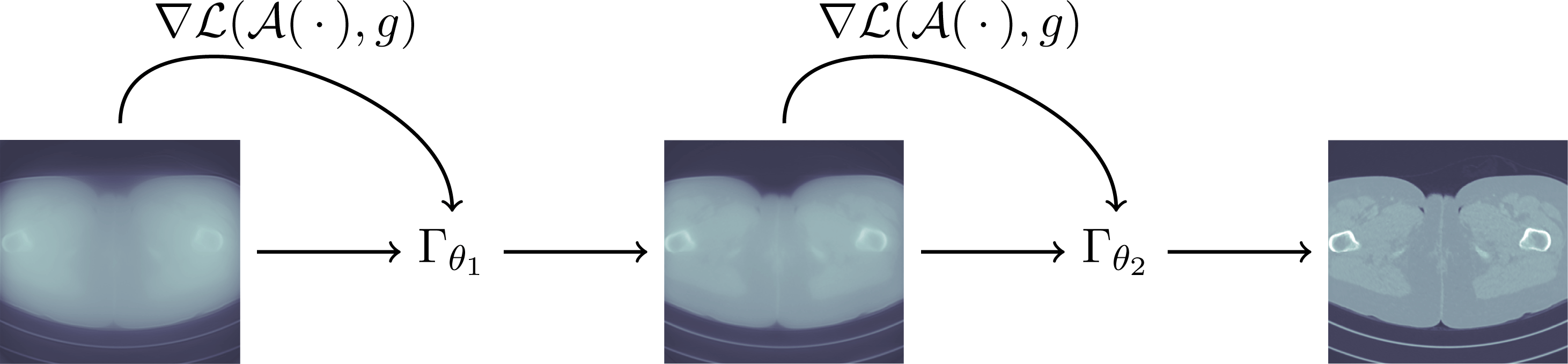
Following Section 4.9.1, the next level of complexity comes when the learned component is allowed to be less constrained by removing the explicit expression for
 $f\mapsto \unicode[STIX]{x1D6FB}{\mathcal{L}}({\mathcal{A}}(f),g)$
in (5.11) while keeping expressions for the forward operator and the adjoint of its derivative. This corresponds to defining
$f\mapsto \unicode[STIX]{x1D6FB}{\mathcal{L}}({\mathcal{A}}(f),g)$
in (5.11) while keeping expressions for the forward operator and the adjoint of its derivative. This corresponds to defining
 ${\mathcal{R}}_{\unicode[STIX]{x1D703}}:Y\rightarrow X$
as in (4.38) but with no memory, that is,
${\mathcal{R}}_{\unicode[STIX]{x1D703}}:Y\rightarrow X$
as in (4.38) but with no memory, that is,
 $$\begin{eqnarray}{\mathcal{R}}_{\unicode[STIX]{x1D703}}(g):=({\mathcal{P}}_{X}\circ \unicode[STIX]{x1D6EC}_{\unicode[STIX]{x1D703}_{N}}\circ \ldots \circ \unicode[STIX]{x1D6EC}_{\unicode[STIX]{x1D703}_{1}})(f^{0},g),\end{eqnarray}$$
where
 ${\mathcal{P}}_{X}:X\times Y\rightarrow X$
is the usual projection and
${\mathcal{P}}_{X}:X\times Y\rightarrow X$
is the usual projection and
 $\unicode[STIX]{x1D6EC}_{\unicode[STIX]{x1D703}_{k}}:X\times Y\rightarrow X\times Y$
for
$\unicode[STIX]{x1D6EC}_{\unicode[STIX]{x1D703}_{k}}:X\times Y\rightarrow X\times Y$
for
 $k=1,\ldots ,N$
is
$k=1,\ldots ,N$
is
 $$\begin{eqnarray}\unicode[STIX]{x1D6EC}_{\unicode[STIX]{x1D703}_{k}}(f,v):=\unicode[STIX]{x1D6E4}_{\unicode[STIX]{x1D703}_{k}}(f,v,[\unicode[STIX]{x2202}\!{\mathcal{A}}(f)]^{\ast }(v),{\mathcal{A}}(f),\unicode[STIX]{x1D6FB}\!{\mathcal{S}}_{\unicode[STIX]{x1D706}}(f))\quad \text{for }(f,v)\in X\times Y.\end{eqnarray}$$
Here,
 $\unicode[STIX]{x1D6E4}_{\unicode[STIX]{x1D703}_{k}}:X\times Y\times X\times Y\times X\rightarrow X\times Y$
is the updating operator that is given by a deep neural network. The resulting deep neural network
$\unicode[STIX]{x1D6E4}_{\unicode[STIX]{x1D703}_{k}}:X\times Y\times X\times Y\times X\rightarrow X\times Y$
is the updating operator that is given by a deep neural network. The resulting deep neural network
 ${\mathcal{R}}_{\unicode[STIX]{x1D703}}:Y\rightarrow X$
is learned from supervised data (5.6) by approximately solving (5.7) using a training algorithm as in (5.8).
${\mathcal{R}}_{\unicode[STIX]{x1D703}}:Y\rightarrow X$
is learned from supervised data (5.6) by approximately solving (5.7) using a training algorithm as in (5.8).
The constraints on the learning can be further decreased, at the expense of increased memory footprint and computational complexity, by allowing for some memory
 $l>0$
, that is, each of the learned updating operators account for more than the previous iterate. This leads to an architecture for
$l>0$
, that is, each of the learned updating operators account for more than the previous iterate. This leads to an architecture for
 ${\mathcal{R}}_{\unicode[STIX]{x1D703}}:Y\rightarrow X$
of the form (4.38) with updating operators as in (4.37). A special case of this formulation is the learned gradient method of Adler and Öktem (Reference Adler and Öktem2017), who in turn present the recurrent inference machines of Putzky and Welling (Reference Putzky and Welling2017) as special case.
${\mathcal{R}}_{\unicode[STIX]{x1D703}}:Y\rightarrow X$
of the form (4.38) with updating operators as in (4.37). A special case of this formulation is the learned gradient method of Adler and Öktem (Reference Adler and Öktem2017), who in turn present the recurrent inference machines of Putzky and Welling (Reference Putzky and Welling2017) as special case.
Another special case is variational networks. These are defined by unrolling an iterative scheme for minimizing an explicit objective that has a data discrepancy component and a regularizer. The idea was introduced by Hammernik et al. (Reference Hammernik, Knoll, Sodickson and Pock2016) for two-dimensional Fourier inversion, where the objective has a regularizer based on a reaction–diffusion model. Hammernik et al. (Reference Hammernik, Klatzer, Kobler, Recht, Sodickson, Pock and Knoll2018) develop it further: they consider a variational network (outlined in their Figure 1) obtained by unrolling the iterations of their equation (6). This corresponds to (5.11) with
 $\unicode[STIX]{x1D6EC}_{\unicode[STIX]{x1D703}_{k}}:X\rightarrow X$
given as
$\unicode[STIX]{x1D6EC}_{\unicode[STIX]{x1D703}_{k}}:X\rightarrow X$
given as
 $$\begin{eqnarray}\unicode[STIX]{x1D6EC}_{\unicode[STIX]{x1D703}_{k}}:=\text{id}+\unicode[STIX]{x1D714}_{k}\unicode[STIX]{x1D6FB}[{\mathcal{L}}({\mathcal{A}}(\,\cdot \,),g)+{\mathcal{S}}_{\unicode[STIX]{x1D719}_{k}}(\,\cdot \,)]\quad \text{for }\unicode[STIX]{x1D703}_{k}=(\unicode[STIX]{x1D714}_{k},\unicode[STIX]{x1D719}_{k}).\end{eqnarray}$$
The regularizer
 ${\mathcal{S}}_{\unicode[STIX]{x1D719}_{k}}:X\rightarrow \mathbb{R}$
is chosen as the FoE model (see also Section 4.3.2):
${\mathcal{S}}_{\unicode[STIX]{x1D719}_{k}}:X\rightarrow \mathbb{R}$
is chosen as the FoE model (see also Section 4.3.2):
 $$\begin{eqnarray}{\mathcal{S}}_{\unicode[STIX]{x1D719}_{k}}(f):=\mathop{\sum }_{j}\unicode[STIX]{x1D6F7}_{k,j}(f\ast K_{k,j})\quad \text{for }\unicode[STIX]{x1D719}_{k}=(\unicode[STIX]{x1D6F7}_{k,j},K_{k,j}),\end{eqnarray}$$
where the (potential) functionals
 $\unicode[STIX]{x1D6F7}_{k,j}:X\rightarrow \mathbb{R}$
and the convolution kernels
$\unicode[STIX]{x1D6F7}_{k,j}:X\rightarrow \mathbb{R}$
and the convolution kernels
 $K_{k,j}\in X$
are all parametrized by finite-dimensional parameters, so
$K_{k,j}\in X$
are all parametrized by finite-dimensional parameters, so
 $\unicode[STIX]{x1D719}_{k}$
is a finite-dimensional parameter. See also Chen et al. (Reference Chen, Zhang, Chen, Zhang, Zhang, Sun, Lv, Liao, Zhou and Wang2019), who essentially apply the approach of Hammernik et al. (Reference Hammernik, Klatzer, Kobler, Recht, Sodickson, Pock and Knoll2018) to CT reconstruction. Another variant of variational networks is that of Bostan, Kamilov and Waller (Reference Bostan, Kamilov and Waller2018), who unroll a proximal algorithm for an objective with a TV regularizer and replace the scalar soft-thresholding function with a parametrized variant (see Bostan et al. Reference Bostan, Kamilov and Waller2018, equation (8)). This yields a proximal algorithm that uses a sequence of adjustable shrinkage functions in addition to self-tuning the step-size. In particular, unlike Mousavi and Baraniuk (Reference Mousavi and Baraniuk2017), the method presented here does not rely on having a structured normal operator. A further variant of a variational network is given by Aggarwal, Mani and Jacob (Reference Aggarwal, Mani and Jacob2019), who unroll a gradient descent scheme for minimizing an objective whose regularizer is given by a CNN (see Aggarwal et al. Reference Aggarwal, Mani and Jacob2019, equation (7)). A similar approach is also considered by Zhao, Zhang, Wang and Gao (Reference Zhao, Zhang, Wang and Gao2018a
), who unroll an ADMM scheme and stop iterates according to a Morozov-type stopping criterion (not a fixed number of iterates), so the number of layers depends on the noise level in data.
$\unicode[STIX]{x1D719}_{k}$
is a finite-dimensional parameter. See also Chen et al. (Reference Chen, Zhang, Chen, Zhang, Zhang, Sun, Lv, Liao, Zhou and Wang2019), who essentially apply the approach of Hammernik et al. (Reference Hammernik, Klatzer, Kobler, Recht, Sodickson, Pock and Knoll2018) to CT reconstruction. Another variant of variational networks is that of Bostan, Kamilov and Waller (Reference Bostan, Kamilov and Waller2018), who unroll a proximal algorithm for an objective with a TV regularizer and replace the scalar soft-thresholding function with a parametrized variant (see Bostan et al. Reference Bostan, Kamilov and Waller2018, equation (8)). This yields a proximal algorithm that uses a sequence of adjustable shrinkage functions in addition to self-tuning the step-size. In particular, unlike Mousavi and Baraniuk (Reference Mousavi and Baraniuk2017), the method presented here does not rely on having a structured normal operator. A further variant of a variational network is given by Aggarwal, Mani and Jacob (Reference Aggarwal, Mani and Jacob2019), who unroll a gradient descent scheme for minimizing an objective whose regularizer is given by a CNN (see Aggarwal et al. Reference Aggarwal, Mani and Jacob2019, equation (7)). A similar approach is also considered by Zhao, Zhang, Wang and Gao (Reference Zhao, Zhang, Wang and Gao2018a
), who unroll an ADMM scheme and stop iterates according to a Morozov-type stopping criterion (not a fixed number of iterates), so the number of layers depends on the noise level in data.
Remark 5.1. An interesting aspect of the variational network of Hammernik et al. (Reference Hammernik, Knoll, Sodickson and Pock2016) is that
 $\unicode[STIX]{x1D6EC}_{\unicode[STIX]{x1D703}_{k}}$
can be interpreted as a gradient descent step in an optimization scheme that minimizes an objective functional
$\unicode[STIX]{x1D6EC}_{\unicode[STIX]{x1D703}_{k}}$
can be interpreted as a gradient descent step in an optimization scheme that minimizes an objective functional
 $f\mapsto {\mathcal{L}}({\mathcal{A}}(f),g)+{\mathcal{S}}_{\unicode[STIX]{x1D719}_{k}}(f)$
. In particular, if
$f\mapsto {\mathcal{L}}({\mathcal{A}}(f),g)+{\mathcal{S}}_{\unicode[STIX]{x1D719}_{k}}(f)$
. In particular, if
 $\unicode[STIX]{x1D719}_{k}$
is the same for all
$\unicode[STIX]{x1D719}_{k}$
is the same for all
 $k$
, then increasing the number of layers by
$k$
, then increasing the number of layers by
 $N\rightarrow \infty$
will in the limit yield a MAP estimator instead of a Bayes estimator.
$N\rightarrow \infty$
will in the limit yield a MAP estimator instead of a Bayes estimator.
Other applications of the learned gradient method include those of Gong et al. (Reference Gong, Zhang, Shi, van den Hengel, Shen and Zhang2018) for deconvolution, Qin et al. (Reference Qin, Schlemper, Caballero, Price, Hajnal and Rueckert2019) for dynamic cardiac two-dimensional MRI (here one needs to exploit the temporal dependence), Hauptmann et al. (Reference Hauptmann, Lucka, Betcke, Huynh, Adler, Cox, Beard, Ourselin and Arridge2018) for three-dimensional PAT, and Wu, Kim and Li (Reference Wu, Kim and Li2018a ) for three-dimensional CT reconstruction. The challenge in three-dimensional applications is to manage the high computational and memory cost for the training of the unrolled network. One approach is to replace the end-to-end training of the entire neural network and instead break down each iteration and train the sub-networks sequentially (gradient boosting). This is the approach taken by Hauptmann et al. (Reference Hauptmann, Lucka, Betcke, Huynh, Adler, Cox, Beard, Ourselin and Arridge2018) and Wu et al. (Reference Wu, Kim and Li2018a ), but as shown by Wu et al. (Reference Wu, Kim and Li2018a ), the output quality has minor improvements over learned post-processing (Section 5.1.5), which also scales to the three-dimensional setting. A better alternative could be to use a reversible residual network architecture (Gomez et al. Reference Gomez, Ren, Urtasun and Grosse2017, Ardizzone et al. Reference Ardizzone, Kruse, Wirkert, Rahner, Pellegrini, Klessen, Maier-Hein, Rother and Köthe2018) for a learned iterative method, since these are much better at managing memory consumption in training (mainly when calculating gradients using backpropagation) as networks grow deeper and wider. However, this is yet to be done.
Learned iterative in both model parameter and data spaces.
The final enhancement to the learned iterative schemes is to introduce an explicit learned updating in the data space as well. To see how this can be achieved, one can unroll a primal–dual-type scheme of the form
 $$\begin{eqnarray}\left\{\begin{array}{@{}ll@{}}v^{0}=g\text{ and }f^{0}\in X\text{ given}\quad & \\ v^{k+1}=\unicode[STIX]{x1D6E4}_{\unicode[STIX]{x1D703}_{k}^{\text{d}}}^{\text{d}}(v^{k},{\mathcal{A}}(f^{k}),g))\quad & \\ f^{k+1}=\unicode[STIX]{x1D6E4}_{\unicode[STIX]{x1D703}_{k}^{\text{m}}}^{\text{m}}(f^{k},[\unicode[STIX]{x2202}{\mathcal{A}}(f)]^{\ast }(v^{k+1}))\quad & \end{array}\right.\quad \text{for }k=0,\ldots ,N-1.\end{eqnarray}$$
Here,
 $$\begin{eqnarray}\unicode[STIX]{x1D6E4}_{\unicode[STIX]{x1D703}_{k}^{\text{m}}}^{\text{m}}:X\times X\rightarrow X\quad \text{and}\quad \unicode[STIX]{x1D6E4}_{\unicode[STIX]{x1D703}_{k}^{\text{d}}}^{\text{d}}:Y\times Y\times Y\rightarrow Y\end{eqnarray}$$
are the updating operators. This corresponds to defining
 ${\mathcal{R}}_{\unicode[STIX]{x1D703}}:Y\rightarrow X$
with
${\mathcal{R}}_{\unicode[STIX]{x1D703}}:Y\rightarrow X$
with
 $\unicode[STIX]{x1D703}_{k}=(\unicode[STIX]{x1D703}_{k}^{\text{m}},\unicode[STIX]{x1D703}_{k}^{\text{d}})$
as in (5.13), where
$\unicode[STIX]{x1D703}_{k}=(\unicode[STIX]{x1D703}_{k}^{\text{m}},\unicode[STIX]{x1D703}_{k}^{\text{d}})$
as in (5.13), where
 $\unicode[STIX]{x1D6EC}_{\unicode[STIX]{x1D703}_{k}}:X\times Y\rightarrow X\times Y$
is given by
$\unicode[STIX]{x1D6EC}_{\unicode[STIX]{x1D703}_{k}}:X\times Y\rightarrow X\times Y$
is given by
 $$\begin{eqnarray}\unicode[STIX]{x1D6EC}_{\unicode[STIX]{x1D703}_{k}}(f,v):=(\unicode[STIX]{x1D6E4}_{\unicode[STIX]{x1D703}_{k}^{\text{m}}}^{\text{m}}(f,[\unicode[STIX]{x2202}{\mathcal{A}}(f)]^{\ast }(\unicode[STIX]{x1D6E4}_{\unicode[STIX]{x1D703}_{k}^{\text{d}}}^{\text{d}}(v,{\mathcal{A}}(f),g))),\unicode[STIX]{x1D6E4}_{\unicode[STIX]{x1D703}_{k}^{\text{d}}}^{\text{data}}(v,{\mathcal{A}}(f),g))).\end{eqnarray}$$
This is illustrated in Figure 5.2, and similar networks are also suggested by Vogel and Pock (Reference Vogel, Pock, Roth and Vetter2017) and Kobler et al. (Reference Kobler, Klatzer, Hammernik and Pock2017), who extend the approach of Hammernik et al. (Reference Hammernik, Klatzer, Kobler, Recht, Sodickson, Pock and Knoll2018) by parametrizing and learning the data discrepancy
 ${\mathcal{L}}$
. Applications are for inverting the two-dimensional Fourier transform (two-dimensional MRI image reconstruction). See also He et al. (Reference He, Yang, Wang, Zeng, Bian, Zhang, Sun, Xu and Ma2019), who unroll an ADMM scheme with updates in both reconstruction and data spaces and apply that to two-dimensional CT reconstruction.
${\mathcal{L}}$
. Applications are for inverting the two-dimensional Fourier transform (two-dimensional MRI image reconstruction). See also He et al. (Reference He, Yang, Wang, Zeng, Bian, Zhang, Sun, Xu and Ma2019), who unroll an ADMM scheme with updates in both reconstruction and data spaces and apply that to two-dimensional CT reconstruction.
Finally, allowing for some memory in both model parameter and data spaces leads to the learned primal–dual scheme of Adler and Öktem (Reference Adler and Öktem2018b ), which is used for low-dose two-dimensional CT reconstruction. The robustness of this approach against uncertainties in the image and uncertainties in system settings is empirically studied by Boink, van Gils, Manohar and Brune (Reference Boink, van Gils, Manohar and Brune2018). The conclusion is that learning improves pure knowledge-based reconstruction in terms of noise removal and background identification, and more variety in the training set increases the robustness against image uncertainty. Robustness against model uncertainty, however, is not readily obtained. An application of a learned primal dual scheme to breast tomosynthesis is given by Moriakov et al. (Reference Moriakov, Michielsen, Adler, Mann, Sechopoulos and Teuwen2018). To outperform existing reconstruction methods, one needs to encode the information about breast thickness into the learned updates for both primal and dual variables.

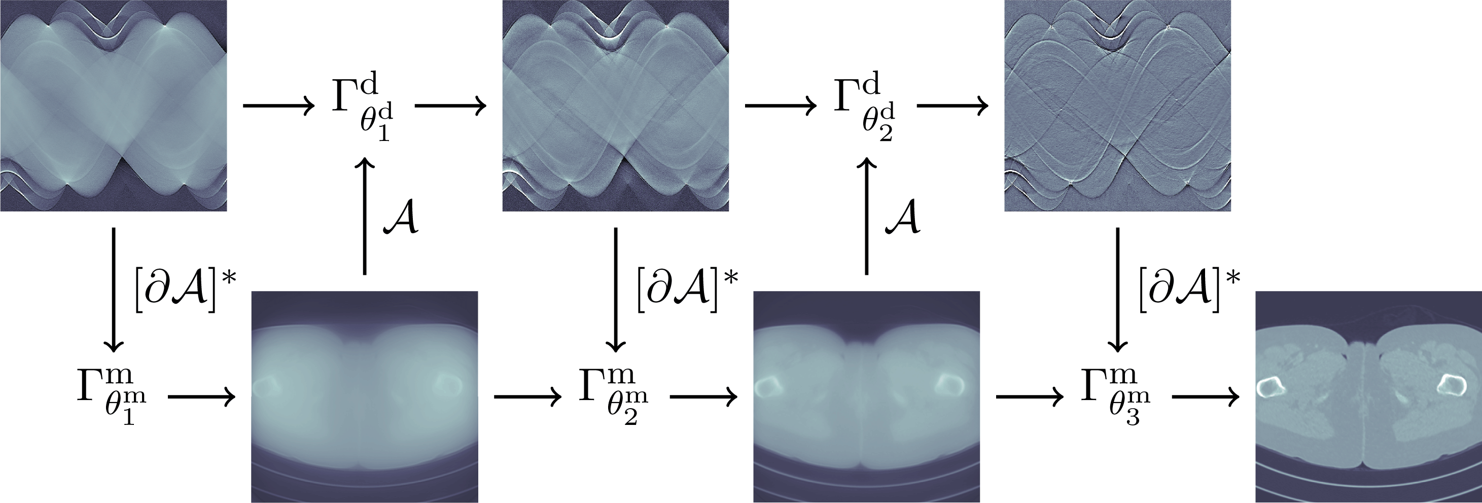
Further remarks.
Successively reducing the constraints on the neural network architecture in the learned iterative scheme allows for larger model capacity, but training such a model also requires more training data. The well-known universal approximation property of deep neural networks (see Cybenko Reference Cybenko1989, Hornik, Stinchcombe and White Reference Hornik, Stinchcombe and White1989, Hornik Reference Hornik1991, Barron Reference Barron1994) implies that the learned iterative schemes in their most unconstrained formulation can approximate a Bayes estimator arbitrarily well given enough supervised data and neural network parameters (model capacity). This does not necessarily hold for the more constrained network architectures, such as those used by the variational networks of Hammernik et al. (Reference Hammernik, Klatzer, Kobler, Recht, Sodickson, Pock and Knoll2018). See also Section 8.2.1 for remarks on approximation properties of certain deep neural networks.
Unrolling an iterative scheme is a central theme in learned iterative methods, and it allows one to construct a deep neural network from an iterative scheme that is stopped after
 $N$
steps. Here, a larger
$N$
steps. Here, a larger
 $N$
simply means adding more layers, i.e. increasing the model capacity. The same idea is used to solve an optimization problem more rapidly (Section 4.9), but here the training is unsupervised and the loss is given by the objective that we seek to minimize. Such an architecture can be used for computing a Bayes estimator when trained using a supervised data or a MAP estimator when trained using unsupervised data. The same holds also for the GAN approach taken in Mardani et al. (Reference Mardani, Gong, Cheng, Vasanawala, Zaharchuk, Alley, Thakur, Han, Dally, Pauly and Xing2017b
) (Section 5.1.6), which uses the same architecture as learned iterative methods but a different loss, that is, it computes a different estimator.
$N$
simply means adding more layers, i.e. increasing the model capacity. The same idea is used to solve an optimization problem more rapidly (Section 4.9), but here the training is unsupervised and the loss is given by the objective that we seek to minimize. Such an architecture can be used for computing a Bayes estimator when trained using a supervised data or a MAP estimator when trained using unsupervised data. The same holds also for the GAN approach taken in Mardani et al. (Reference Mardani, Gong, Cheng, Vasanawala, Zaharchuk, Alley, Thakur, Han, Dally, Pauly and Xing2017b
) (Section 5.1.6), which uses the same architecture as learned iterative methods but a different loss, that is, it computes a different estimator.
5.1.5 Learned post- and/or pre-processing
One of the earliest applications of deep learning in inverse problems in imaging was as a post-processing tool. Here, an established non-learned reconstruction method is followed by a deep neural network that is trained to ‘clean up’ noise and artefacts introduced by the first inversion step. The first inversion step is typically performed using a pseudo-inverse of the forward operator, e.g. backprojection or FBP in CT or a zero-filling solution in MRI. This initial reconstruction method can be seen as a way to account for how data are generated, whereas the learning part acts only on the model parameter instead of data.
As one might expect, a vast number of papers apply deep learning to images obtained from some kind of image reconstruction. In principle, all of these qualify as a learned post-processing scheme. We will not attempt to prove a (near-complete) survey of these since the learning part is not directly related to the inverse problem. Instead we mention some key publications from imaging that have image reconstruction as their main theme, followed by a characterization of the estimator one seeks to approximate when using learned post-processing.
Selected publications focusing on image reconstruction.
We start with surveying work related to learned post-processing for CT image reconstruction. Early approaches used a CNN to map a sparse-view CT reconstruction to a full-view one, as in Zhao, Chen, Zhang and Jin (Reference Zhao, Chen, Zhang and Jin2016). A similar approach to mapping low-dose CT images to normal-dose images (denoising) is that of Chen et al. (Reference Chen, Zhang, Zhang, Liao, Li, Zhou and Wang2017b ), who train a CNN on image patches. See also Chen et al. (Reference Chen, Zhang, Kalra, Lin, Chen, Liao, Zhou and Wang2017a ) for an approach that uses a residual encoder–decoder CNN (RED-CNN) trained on image patches for the same purpose.
Denoising low-dose CT images can also be done using a U-Net, as in Jin, McCann, Froustey and Unser (Reference Jin, McCann, Froustey and Unser2017). Another variant is to use the U-Net on directional wavelets (AAPM-Net), as in Kang, Min and Ye (Reference Kang, Min and Ye2017). This method came second in the 2016 AAPM Low Dose CT Grand Challenge.Footnote 6 It has since been further developed and refined in a series of publications: for example, Kang, Chang, Yoo and Ye (Reference Kang, Chang, Yoo and Ye2018) and Kang and Ye (Reference Kang and Ye2018) modify the AAPM-Net architecture by using a wavelet residual network (WavResNet), which is a deep CNN reinterpreted as cascaded convolution framelet signal representation. Another drawback of AAPM-Net is that it does not satisfy the frame condition and it overly emphasizes the low-frequency component of the signal, which leads to blurring artefacts in the post-processed CT images. To address this, Han and Ye (Reference Han and Ye2018) suggest a U-Net-based network architecture with directional wavelets that satisfy the frame condition. Finally, Ye et al. (Reference Ye, Han and Cha2018) develop a mathematical framework to understand deep learning approaches for inverse problems based on these deep convolutional framelets. Such architectures represent a signal decomposition similar to using wavelets or framelets, but here the basis is learned from the training data. This idea of using techniques from applied harmonic analysis and sparse signal processing to analyse approximation properties of certain classes of deep neural networks bears similarities to Bölcskei, Grohs, Kutyniok and Petersen (Reference Bölcskei, Grohs, Kutyniok and Petersen2019) (see Section 8.2.1) and the scattering networks discussed in Section 4.5 as well as work related to multi-layer convolutional sparse coding outlined in Section 4.4.2.
Yet another CNN architecture (Mixed-Scale Dense CNN) is proposed in Pelt, Batenburg and Sethian (Reference Pelt, Batenburg and Sethian2018) for denoising and removing streak artefacts from limited angle CT reconstructions. Empirical evidence shows that this architecture comes with some advantages over encoder–decoder networks. It can be trained on relatively small training sets and the same hyper-parameters in training can often be re-used across a wide variety of problems. This removes the need to perform a time-consuming trial-and-error search for hyper-parameter values.
Besides architectures, one may also consider the choice of loss function, as in Zhang et al. (Reference Zhang, Liang, Dong, Xie and Cao2018), who consider CNN-based denoising of CT images using a loss function that is a linear combination of squared
 $L^{2}$
and multi-scale scale structural similarity index (SSIM). A closely related work is that of Zhang and Yu (Reference Zhang and Yu2018), which uses a CNN trained on image patches with a loss function that is a sum of squared
$L^{2}$
and multi-scale scale structural similarity index (SSIM). A closely related work is that of Zhang and Yu (Reference Zhang and Yu2018), which uses a CNN trained on image patches with a loss function that is a sum of squared
 $L^{2}$
losses over the patches. The aim here is to reduce streak artefacts from highly scattering media, such as metal implants. A number of papers use techniques from GANs to post-process CT images. Shan et al. (Reference Shan, Zhang, Yang, Kruger, Kalra, Sun, Cong and Wang2018) use a conveying path-based convolutional encoder–decoder network. A novel feature of this approach is that an initial three-dimensional denoising model can be directly obtained by extending a trained two-dimensional CNN, which is then fine-tuned to incorporate three-dimensional spatial information from adjacent slices (transfer learning from two to three dimensions). The paper also contains a summary of deep learning network architectures for CT post-processing listing the loss function (squared
$L^{2}$
losses over the patches. The aim here is to reduce streak artefacts from highly scattering media, such as metal implants. A number of papers use techniques from GANs to post-process CT images. Shan et al. (Reference Shan, Zhang, Yang, Kruger, Kalra, Sun, Cong and Wang2018) use a conveying path-based convolutional encoder–decoder network. A novel feature of this approach is that an initial three-dimensional denoising model can be directly obtained by extending a trained two-dimensional CNN, which is then fine-tuned to incorporate three-dimensional spatial information from adjacent slices (transfer learning from two to three dimensions). The paper also contains a summary of deep learning network architectures for CT post-processing listing the loss function (squared
 $L^{2}$
, adversarial or perpetual loss). A similar approach is taken by Yang et al. (Reference Yang, Yan, Zhang, Yu, Shi, Mou, Kalra, Zhang, Sun and Wang2018c
), who denoise CT images via a GAN with Wasserstein distance and perceptual similarity. The perceptual loss suppresses noise by comparing the perceptual features of a denoised output against those of the ground truth in an established feature space, while the generator focuses more on migrating the data noise distribution. Another approach is that of You et al. (Reference You, Li, Zhang, Zhang, Shan, Ju, Zhao, Zhang, Cong, Vannier, Saha and Wang2018a
), who use a generator from a GAN to generate high-resolution CT images from low-resolution counterparts. The model is trained on semi-supervised training data and the training is regularized by enforcing a cycle-consistency expressed in terms of the Wasserstein distance. See also You et al. (Reference You, Yang, Shan, Gjesteby, Li, Ju, Zhang, Zhao, Zhang, Cong and Wang2018b
) for similar work, along with an investigation of the impact of different loss functions for training the GAN.
$L^{2}$
, adversarial or perpetual loss). A similar approach is taken by Yang et al. (Reference Yang, Yan, Zhang, Yu, Shi, Mou, Kalra, Zhang, Sun and Wang2018c
), who denoise CT images via a GAN with Wasserstein distance and perceptual similarity. The perceptual loss suppresses noise by comparing the perceptual features of a denoised output against those of the ground truth in an established feature space, while the generator focuses more on migrating the data noise distribution. Another approach is that of You et al. (Reference You, Li, Zhang, Zhang, Shan, Ju, Zhao, Zhang, Cong, Vannier, Saha and Wang2018a
), who use a generator from a GAN to generate high-resolution CT images from low-resolution counterparts. The model is trained on semi-supervised training data and the training is regularized by enforcing a cycle-consistency expressed in terms of the Wasserstein distance. See also You et al. (Reference You, Yang, Shan, Gjesteby, Li, Ju, Zhang, Zhao, Zhang, Cong and Wang2018b
) for similar work, along with an investigation of the impact of different loss functions for training the GAN.
For PET image reconstruction, da Luis and Reader (Reference da Luis and Reader2017) use a CNN to denoise PET reconstructions obtained by ML-EM. A more involved approach is presented in Yang, Ying and Tang (Reference Yang, Ying and Tang2018a ), which learns a post-processing step for enhancing PET reconstructions obtained by MAP with a Green smoothness prior (see Yang et al. Reference Yang, Ying and Tang2018a , equation (6)). More precisely, this is supervised training on tuples consisting of ground truth and a number of MAP solutions where one varies parameters defining the prior. The training seeks to learn a mapping that takes a set of small image patches at the same location from the MAP solutions to the corresponding patch in the ground truth, thereby resulting in a learned patch-based image denoising scheme. A related approach is that of Kim et al. (Reference Kim, Wu, Gong, Dutta, Kim, Son, Kim, Fakhri and Li2018), who train a CNN to map low-dose PET images to a full-dose one. Both low-dose and full-dose reconstructions are obtained using ordered subsets ML-EM. Since the resulting trained CNN denoiser produces additional bias induced by the disparity of noise levels, one considers learning a regularizer that includes the CNN denoiser (see Kim et al. Reference Kim, Wu, Gong, Dutta, Kim, Son, Kim, Fakhri and Li2018, equation (8)). The resulting variational problem is solved using the ADMM method.
Concerning MRI, most learned post-processing applications seek to train a mapping that takes a zero-filling reconstructionFootnote 7 obtained from under-sampled MRI data to the MRI reconstruction that corresponds to fully sampled data. For example, Wang et al. (Reference Wang, Su, Ying, Peng, Zhu, Liang, Feng and Liang2016) use a CNN for this purpose, and the deep learning output is either used as an initialization or as a regularization term in classical compressed sensing approaches to MRI image reconstruction. Another example is that of Hyun et al. (Reference Hyun, Kim, Lee, Lee and Seo2018), who use a CNN to process a zero-filling reconstruction followed by a particular k-space correction. This outperforms plain zero-filling reconstruction as well as learned post-processing where Fourier inversion is combined with a trained denoiser based on a plain U-Net architecture.
Similar to CT image processing, there has been some work on using GANs to post-process MRI reconstructions. One example is that of Quan, Member, Nguyen-Duc and Jeong (Reference Quan, Member, Nguyen-Duc and Jeong2018), who use a generator within a GAN setting to learn a post-processing operator that maps a zero-filling reconstruction image to a full reconstruction image. Training is regularized using a loss that includes a cyclic loss consistency term that promotes accurate interpolation of the given under-sampled k-space data. The generator consists of multiple end-to-end networks chained together, where the first network translates a zero-filling reconstruction image to a full reconstruction image, and the following networks improve accuracy of the full reconstruction image (refinement step). Another approach using a generator from a trained GAN is given by Yang et al. (Reference Yang, Yu, Dong, Slabaugh, Dragotti, Ye, Liu, Arridge, Keegan, Guo and Firmin2018b
), who use a U-Net architecture with skip connections for the generator. The loss consists of an adversarial loss term, a novel content loss term considering both squared
 $L^{2}$
and a perceptual loss term defined by pre-trained deep convolutional networks. There is also a squared
$L^{2}$
and a perceptual loss term defined by pre-trained deep convolutional networks. There is also a squared
 $L^{2}$
in both model parameter and data spaces, and the latter involves applying the forward operator to the training data to evaluate the squared
$L^{2}$
in both model parameter and data spaces, and the latter involves applying the forward operator to the training data to evaluate the squared
 $L^{2}$
in data space. See Yang et al. (Reference Yang, Yu, Dong, Slabaugh, Dragotti, Ye, Liu, Arridge, Keegan, Guo and Firmin2018b
, equation (13)) for the full expression.
$L^{2}$
in data space. See Yang et al. (Reference Yang, Yu, Dong, Slabaugh, Dragotti, Ye, Liu, Arridge, Keegan, Guo and Firmin2018b
, equation (13)) for the full expression.
We conclude by mentioning some approaches that involve pre-processing. For CT imaging, deep-learning-based pre-processing targets sinogram in-painting, which is the task of mapping observed, sparsely sampled, CT projection data onto corresponding densely sampled CT projection data. Lee et al. (Reference Lee, Lee, Kim, Cho and Cho2019) achieve this via a plain CNN whereas Ghani and Karl (Reference Ghani and Karl2018) use a generator from a trained conditional GAN. A CNN is also used by Hong et al. (Reference Hong, Zan, Weng, Tao, Peng and Huang2018) to pre-process PET data. Here one uses a deep residual CNN for PET super-resolution, that is, to map PET sinogram data from a scanner with large pixellated crystals to one with small pixellated crystals. The CNN-based method was designed and applied as an intermediate step between the projection data acquisition and the image reconstruction. Results are validated using both analytically simulated data, Monte Carlo simulated data and experimental pre-clinical data. In a similar manner, Allman, Reiter and Bell (Reference Allman, Reiter and Bell2018) use a CNN to pre-process photoacoustic data to identify and remove noise artefacts. Finally, we cite Huizhuo, Jinzhu and Zhanxing (Reference Huizhuo, Jinzhu and Zhanxing2018), who use a CNN to jointly pre- and post-process CT data and images. The pre-processing amounts to sinogram in-painting and the post-processing is image denoising, and the middle reconstruction step is performed using FBP. The loss function for this joint pre- and post-processing scheme is given in Huizhuo et al. (Reference Huizhuo, Jinzhu and Zhanxing2018, equation (3)).
Characterizing the estimator.
Here we consider post-processing; one can make analogous arguments for pre-processing. To understand what learned post-processing computes, consider the supervised learning setting. Learned post-processing seeks to approximate the Bayes estimator for the model parameter conditioned on the initial reconstruction, which is a different estimator from the one considered in deep direct Bayes estimation (Sections 5.1.2–5.1.4).
Stated formally, let
 $\unicode[STIX]{x1D559}$
be a
$\unicode[STIX]{x1D559}$
be a
 $X$
-valued random variable defined as
$X$
-valued random variable defined as
 $\unicode[STIX]{x1D559}:=\{^{\dagger }(\unicode[STIX]{x1D558})$
, where
$\unicode[STIX]{x1D559}:=\{^{\dagger }(\unicode[STIX]{x1D558})$
, where
 $\unicode[STIX]{x1D558}$
is the
$\unicode[STIX]{x1D558}$
is the
 $Y$
-valued random variable generating data. Also, let
$Y$
-valued random variable generating data. Also, let
 $\{^{\dagger }:Y\rightarrow X$
denote the fixed initial reconstruction operator that is not learned. We now seek the Bayes estimator for the conditional random variable
$\{^{\dagger }:Y\rightarrow X$
denote the fixed initial reconstruction operator that is not learned. We now seek the Bayes estimator for the conditional random variable
 $(\unicode[STIX]{x1D557}\mid \unicode[STIX]{x1D559}=h)$
, where
$(\unicode[STIX]{x1D557}\mid \unicode[STIX]{x1D559}=h)$
, where
 $h=\{^{\dagger }(g)$
with data
$h=\{^{\dagger }(g)$
with data
 $g\in Y$
being a single sample of
$g\in Y$
being a single sample of
 $\unicode[STIX]{x1D558}$
. This yields a reconstruction operator
$\unicode[STIX]{x1D558}$
. This yields a reconstruction operator
 ${\mathcal{R}}:Y\rightarrow X$
given as
${\mathcal{R}}:Y\rightarrow X$
given as
 ${\mathcal{R}}:={\mathcal{B}}_{\unicode[STIX]{x1D70E}}\circ \{^{\dagger }$
with
${\mathcal{R}}:={\mathcal{B}}_{\unicode[STIX]{x1D70E}}\circ \{^{\dagger }$
with
 ${\mathcal{B}}_{\unicode[STIX]{x1D70E}}:X\rightarrow X$
solving
${\mathcal{B}}_{\unicode[STIX]{x1D70E}}:X\rightarrow X$
solving
where
 $\ell _{X}:X\times X\rightarrow \mathbb{R}$
is a fixed loss function. In the above,
$\ell _{X}:X\times X\rightarrow \mathbb{R}$
is a fixed loss function. In the above,
 $\unicode[STIX]{x1D70E}$
denotes the joint law for
$\unicode[STIX]{x1D70E}$
denotes the joint law for
 $(\unicode[STIX]{x1D557},\unicode[STIX]{x1D559})$
, which is clearly unknown. It can, however, be replaced by its empirical counterpart given from supervised training data,
$(\unicode[STIX]{x1D557},\unicode[STIX]{x1D559})$
, which is clearly unknown. It can, however, be replaced by its empirical counterpart given from supervised training data,
 $$\begin{eqnarray}\unicode[STIX]{x1D6F4}_{m}:=\{(f_{1},h_{1}),\ldots ,(f_{m},h_{m})\}\subset X\times X,\end{eqnarray}$$
where
 $(f_{i},h_{i})$
are generated by
$(f_{i},h_{i})$
are generated by
 $(\unicode[STIX]{x1D557},\unicode[STIX]{x1D559})\sim \unicode[STIX]{x1D70E}$
. Furthermore, considering all possible estimators (non-randomized decision rules)
$(\unicode[STIX]{x1D557},\unicode[STIX]{x1D559})\sim \unicode[STIX]{x1D70E}$
. Furthermore, considering all possible estimators (non-randomized decision rules)
 ${\mathcal{B}}:X\rightarrow X$
in the minimization in (5.16) is computationally unfeasible. To address this, we consider a family
${\mathcal{B}}:X\rightarrow X$
in the minimization in (5.16) is computationally unfeasible. To address this, we consider a family
 $\{{{\mathcal{B}}_{\unicode[STIX]{x1D703}}\}}_{\unicode[STIX]{x1D703}\in \unicode[STIX]{x1D6E9}}$
of estimators that is parametrized by a finite-dimensional parameter in
$\{{{\mathcal{B}}_{\unicode[STIX]{x1D703}}\}}_{\unicode[STIX]{x1D703}\in \unicode[STIX]{x1D6E9}}$
of estimators that is parametrized by a finite-dimensional parameter in
 $\unicode[STIX]{x1D6E9}$
. Restricting attention to such a parametrized family of estimators yields the following empirical risk minimization problem:
$\unicode[STIX]{x1D6E9}$
. Restricting attention to such a parametrized family of estimators yields the following empirical risk minimization problem:
with
 $(f_{i},h_{i})\in \unicode[STIX]{x1D6F4}_{m}$
as in (5.17).
$(f_{i},h_{i})\in \unicode[STIX]{x1D6F4}_{m}$
as in (5.17).
Now, consider the case when the initial reconstruction method
 $\{^{\dagger }:Y\rightarrow X$
is a linear sufficient statistic, that is,
$\{^{\dagger }:Y\rightarrow X$
is a linear sufficient statistic, that is,
 $$\begin{eqnarray}\mathbb{E}[\unicode[STIX]{x1D557}\mid \unicode[STIX]{x1D558}=g]=\mathbb{E}[\unicode[STIX]{x1D557}\mid \{^{\dagger }(\unicode[STIX]{x1D558})=\{^{\dagger }(g)].\end{eqnarray}$$
For example, the operators given by the FBP and the backprojection are both linear sufficient statistics. If in addition the loss function is the squared
 $L^{2}$
-norm, then
$L^{2}$
-norm, then
 ${\mathcal{R}}:={\mathcal{B}}_{\unicode[STIX]{x1D70E}}\circ \{^{\dagger }$
is also a Bayes estimator for
${\mathcal{R}}:={\mathcal{B}}_{\unicode[STIX]{x1D70E}}\circ \{^{\dagger }$
is also a Bayes estimator for
 $(\unicode[STIX]{x1D557}\mid \unicode[STIX]{x1D558}=g)$
, that is, the reconstruction obtained from learned post-processing coincides with the one from deep direct Bayes estimation. Note, however, that this holds in the limit of infinite amount of training data and infinite model capacity. In fact, as we shall see in Section 7.3, when applied to finite number of training data and finite model capacity, learned post-processing differs from deep direct Bayes estimation.
$(\unicode[STIX]{x1D557}\mid \unicode[STIX]{x1D558}=g)$
, that is, the reconstruction obtained from learned post-processing coincides with the one from deep direct Bayes estimation. Note, however, that this holds in the limit of infinite amount of training data and infinite model capacity. In fact, as we shall see in Section 7.3, when applied to finite number of training data and finite model capacity, learned post-processing differs from deep direct Bayes estimation.
5.1.6 Other estimators
Learning using a supervised GAN.
Some recent work uses a GAN in a supervised learning setting, which leads to a training problem of the type (5.3). For example, Mardani et al. (Reference Mardani, Gong, Cheng, Vasanawala, Zaharchuk, Alley, Thakur, Han, Dally, Pauly and Xing2017b
) defines the variant of (5.3) where
 $\ell _{X}$
is the
$\ell _{X}$
is the
 $L^{1}$
-norm,
$L^{1}$
-norm,
 $\ell _{\mathscr{P}_{X}}$
is the Pearson
$\ell _{\mathscr{P}_{X}}$
is the Pearson
 $\unicode[STIX]{x1D712}^{2}$
-divergence, which can be evaluated using a least-squares GAN (Mao et al.
Reference Mao, Li, Xie, Lau, Wang and Smolley2016), and
$\unicode[STIX]{x1D712}^{2}$
-divergence, which can be evaluated using a least-squares GAN (Mao et al.
Reference Mao, Li, Xie, Lau, Wang and Smolley2016), and
 ${\mathcal{R}}_{\unicode[STIX]{x1D703}}:Y\rightarrow X$
is given by an architecture adapted to MRI. Use of a 1-norm in the generator loss motivates the reference made to ‘compressed sensing’ made by the authors. See also Mardani et al. (Reference Mardani, Gong, Cheng, Pauly and Xing2017a
) and Schwab, Antholzer and Haltmeier (Reference Schwab, Antholzer and Haltmeier2018) for further work along these lines: for example, Schwab et al. (Reference Schwab, Antholzer and Haltmeier2018) more formally treat the manifold projection step that in Mardani et al. (Reference Mardani, Gong, Cheng, Vasanawala, Zaharchuk, Alley, Thakur, Han, Dally, Pauly and Xing2017b
) is specially tailored for MRI imaging.
${\mathcal{R}}_{\unicode[STIX]{x1D703}}:Y\rightarrow X$
is given by an architecture adapted to MRI. Use of a 1-norm in the generator loss motivates the reference made to ‘compressed sensing’ made by the authors. See also Mardani et al. (Reference Mardani, Gong, Cheng, Pauly and Xing2017a
) and Schwab, Antholzer and Haltmeier (Reference Schwab, Antholzer and Haltmeier2018) for further work along these lines: for example, Schwab et al. (Reference Schwab, Antholzer and Haltmeier2018) more formally treat the manifold projection step that in Mardani et al. (Reference Mardani, Gong, Cheng, Vasanawala, Zaharchuk, Alley, Thakur, Han, Dally, Pauly and Xing2017b
) is specially tailored for MRI imaging.
It is not easy to identify what estimator the above really corresponds to, but clearly the generator (after training) resembles a MAP estimator where the prior is given implicitly by the supervised training data. To some extent, one may view the above as a supervised variant of Section 4.7 that uses a GAN to learn a regularizer (prior) from unsupervised data.
Deep direct estimation of higher-order moments.
As described in Adler and Öktem (Reference Adler and Öktem2018a ), one can train a deep neural network to directly approximate an estimator involving higher-order moments, such as pointwise variance and correlation. The starting point is the well-known result
 $$\begin{eqnarray}\mathbb{E}_{\unicode[STIX]{x1D568}}[\unicode[STIX]{x1D568}\mid \unicode[STIX]{x1D558}=\,\cdot \,]=\min _{\operatorname{h}:Y\rightarrow W}\mathbb{E}_{(\unicode[STIX]{x1D558},\unicode[STIX]{x1D568})}[\Vert \operatorname{h}(\unicode[STIX]{x1D558})-\unicode[STIX]{x1D568}\Vert _{W}^{2}].\end{eqnarray}$$
In the above,
 $\unicode[STIX]{x1D568}$
is any random variable taking values in some measurable Banach space
$\unicode[STIX]{x1D568}$
is any random variable taking values in some measurable Banach space
 $W$
and the minimization is over all
$W$
and the minimization is over all
 $W$
-valued measurable maps on
$W$
-valued measurable maps on
 $Y$
. This is useful since many estimators relevant for uncertainty quantification are expressible using terms of this form for appropriate choices of
$Y$
. This is useful since many estimators relevant for uncertainty quantification are expressible using terms of this form for appropriate choices of
 $\unicode[STIX]{x1D568}$
.
$\unicode[STIX]{x1D568}$
.
Specifically, Adler and Öktem (Reference Adler and Öktem2018a
) consider two (deep) neural networks
 ${\mathcal{R}}_{\unicode[STIX]{x1D703}^{\ast }}:Y\rightarrow X$
and
${\mathcal{R}}_{\unicode[STIX]{x1D703}^{\ast }}:Y\rightarrow X$
and
 $\operatorname{h}_{\unicode[STIX]{x1D719}^{\ast }}:Y\rightarrow X$
with appropriate architectures that are trained according to
$\operatorname{h}_{\unicode[STIX]{x1D719}^{\ast }}:Y\rightarrow X$
with appropriate architectures that are trained according to

The joint law
 $\unicode[STIX]{x1D707}$
above can be replaced by its empirical counterpart given from supervised training data
$\unicode[STIX]{x1D707}$
above can be replaced by its empirical counterpart given from supervised training data
 $(f_{i},g_{i})$
, so the
$(f_{i},g_{i})$
, so the
 $\unicode[STIX]{x1D707}$
-expectation is replaced by an averaging over training data. The resulting networks will then approximate the conditional mean and the conditional pointwise variance, respectively.
$\unicode[STIX]{x1D707}$
-expectation is replaced by an averaging over training data. The resulting networks will then approximate the conditional mean and the conditional pointwise variance, respectively.
As already shown, by using (5.19) it is possible to rewrite many estimators as minimizers of an expectation. Such estimators can then be approximated using the direct estimation approach outlined here. This should coincide with computing the same estimator by posterior sampling (Section 5.2.1). Direct estimation is significantly faster, but not as flexible as posterior sampling since each estimator requires a new neural network that specifically trained for that estimator. Section 7.7 compares the outcomes of the two approaches.
5.2 Deep posterior sampling
The idea here is to use techniques from deep learning to sample from the posterior. This can then be used to perform various statistical computations relevant to solving the inverse problem.
Approaches to sampling from high-dimensional distributions that do not use neural networks are very briefly surveyed in Section 3.5.2. A drawback of these approaches is that they require access to an explicit prior, so they do not apply to cases where no explicit prior is available. Furthermore, despite significant algorithmic advances, these methods do not offer computationally feasible means for sampling from the posterior in large-scale inverse problems, such as those arising in three-dimensional imaging. Here we survey an alternative method that uses conditional GAN for the same purpose (Section 5.2.1). This approach has very desirable properties, so it does not require access to an explicit prior, and it is computationally very efficient.
Remark 5.2. Deep Gaussian mixture models (Viroli and McLachlan Reference Viroli and McLachlan2017) are multi-layered networks where the variables at each layer follow a mixture of Gaussian distributions. Hence, the resulting deep mixture model consists of a set of nested (non-linear) mixtures of linear models. Such models can be shown to be universal approximators of probability densities and they can be trained using ML-EM techniques. This is an interesting approach for sampling from the posterior in Bayesian inversion, but it is yet to be used in this context.
Recent work using conditional GAN for the same purpose (Section 5.2.1) gives very promising results. We do not cover deep Gaussian mixture models (Viroli and McLachlan Reference Viroli and McLachlan2017), which are multi-layered networks where, at each layer, the variables follow a mixture of Gaussian distributions. Thus, the deep mixture model consists of a set of nested mixtures of linear models, which globally provide a non-linear model able to describe the data in a very flexible way. These are universal approximators of probability densities that are trainable using ML-EM techniques. This is an interesting approach that is yet to be used in the context of inverse problems.
5.2.1 Conditional GAN
The approach taken was first introduced by Adler and Öktem (Reference Adler and Öktem2018a ), and it is a special case of variational Bayes inference (Section 3.5.2) where the variational family is parametrized via GAN. More precisely, the idea is to explore the posterior by sampling from a generator that has been trained using a conditional Wasserstein GAN discriminator.
To describe how a Wasserstein GAN can be used for this purpose, let data
 $g\in Y$
be fixed and assume that
$g\in Y$
be fixed and assume that
 $\unicode[STIX]{x1D6F1}_{\text{post}}^{g}$
, the posterior of
$\unicode[STIX]{x1D6F1}_{\text{post}}^{g}$
, the posterior of
 $\unicode[STIX]{x1D557}$
at
$\unicode[STIX]{x1D557}$
at
 $\unicode[STIX]{x1D558}=g$
, can be approximated by elements in a parametrized family
$\unicode[STIX]{x1D558}=g$
, can be approximated by elements in a parametrized family
 $\{{\mathcal{G}}_{\unicode[STIX]{x1D703}}(g)\}_{\unicode[STIX]{x1D703}\in \unicode[STIX]{x1D6E9}}$
of probability measures on
$\{{\mathcal{G}}_{\unicode[STIX]{x1D703}}(g)\}_{\unicode[STIX]{x1D703}\in \unicode[STIX]{x1D6E9}}$
of probability measures on
 $X$
. The best such approximation is defined as
$X$
. The best such approximation is defined as
 ${\mathcal{G}}_{\unicode[STIX]{x1D703}^{\ast }}(g)$
, where
${\mathcal{G}}_{\unicode[STIX]{x1D703}^{\ast }}(g)$
, where
 $\unicode[STIX]{x1D703}^{\ast }\in \unicode[STIX]{x1D6E9}$
solves
$\unicode[STIX]{x1D703}^{\ast }\in \unicode[STIX]{x1D6E9}$
solves
Here,
 $\ell _{\mathscr{P}_{X}}:\mathscr{P}_{X}\times \mathscr{P}_{X}\rightarrow \mathbb{R}$
quantifies the ‘distance’ between two probability measures on
$\ell _{\mathscr{P}_{X}}:\mathscr{P}_{X}\times \mathscr{P}_{X}\rightarrow \mathbb{R}$
quantifies the ‘distance’ between two probability measures on
 $X$
. We are, however, interested in the best approximation for ‘all data’, so we extend (5.20) by including an averaging over all possible data. The next step is to choose a distance notion
$X$
. We are, however, interested in the best approximation for ‘all data’, so we extend (5.20) by including an averaging over all possible data. The next step is to choose a distance notion
 $\ell$
that is desirable from both a theoretical and a computational point of view. For example, the distance should be finite, and computational feasibility requires it to be differentiable almost everywhere, since this opens up using stochastic gradient descent (SGD)-type schemes. The Wasserstein 1-distance
$\ell$
that is desirable from both a theoretical and a computational point of view. For example, the distance should be finite, and computational feasibility requires it to be differentiable almost everywhere, since this opens up using stochastic gradient descent (SGD)-type schemes. The Wasserstein 1-distance
 ${\mathcal{W}}$
(Section B.) has these properties (Arjovsky et al.
Reference Arjovsky, Chintala and Bottou2017), and sampling from the posterior
${\mathcal{W}}$
(Section B.) has these properties (Arjovsky et al.
Reference Arjovsky, Chintala and Bottou2017), and sampling from the posterior
 $\unicode[STIX]{x1D6F1}_{\text{post}}^{g}$
can then be replaced by sampling from the probability distribution
$\unicode[STIX]{x1D6F1}_{\text{post}}^{g}$
can then be replaced by sampling from the probability distribution
 ${\mathcal{G}}_{\unicode[STIX]{x1D703}^{\ast }}(g)$
, where
${\mathcal{G}}_{\unicode[STIX]{x1D703}^{\ast }}(g)$
, where
 $\unicode[STIX]{x1D703}^{\ast }$
solves
$\unicode[STIX]{x1D703}^{\ast }$
solves
In the above,
 $\unicode[STIX]{x1D70E}$
is the probability distribution for data and the random variable
$\unicode[STIX]{x1D70E}$
is the probability distribution for data and the random variable
 $\unicode[STIX]{x1D558}\sim \unicode[STIX]{x1D70E}$
generates data.
$\unicode[STIX]{x1D558}\sim \unicode[STIX]{x1D70E}$
generates data.
Observe now that evaluating the objective in (5.21) requires access to the very posterior that we seek to approximate. Furthermore, the distribution
 $\unicode[STIX]{x1D70E}$
of data is often unknown, so an approach based on (5.21) is essentially useless if the purpose is to sample from an unknown posterior. Finally, evaluating the Wasserstein 1-distance directly from its definition is not computationally feasible.
$\unicode[STIX]{x1D70E}$
of data is often unknown, so an approach based on (5.21) is essentially useless if the purpose is to sample from an unknown posterior. Finally, evaluating the Wasserstein 1-distance directly from its definition is not computationally feasible.
On the other hand, as we shall see, all of these drawbacks can be circumvented by rewriting (5.21) as an expectation over the joint law
 $(\unicode[STIX]{x1D557},\unicode[STIX]{x1D558})\sim \unicode[STIX]{x1D707}$
. This makes use of the Kantorovich–Rubinstein duality for the Wasserstein 1-distance (see (B.2)), and one obtains the following approximate version of (5.21):
$(\unicode[STIX]{x1D557},\unicode[STIX]{x1D558})\sim \unicode[STIX]{x1D707}$
. This makes use of the Kantorovich–Rubinstein duality for the Wasserstein 1-distance (see (B.2)), and one obtains the following approximate version of (5.21):
Here,
 $\operatorname{G}_{\unicode[STIX]{x1D703}}:Z\times Y\rightarrow X$
(generator) is a deterministic mapping such that
$\operatorname{G}_{\unicode[STIX]{x1D703}}:Z\times Y\rightarrow X$
(generator) is a deterministic mapping such that
 $\operatorname{G}_{\unicode[STIX]{x1D703}}(\unicode[STIX]{x1D56B},g)\sim {\mathcal{G}}_{\unicode[STIX]{x1D703}}(g)$
, where
$\operatorname{G}_{\unicode[STIX]{x1D703}}(\unicode[STIX]{x1D56B},g)\sim {\mathcal{G}}_{\unicode[STIX]{x1D703}}(g)$
, where
 $\unicode[STIX]{x1D56B}\sim \unicode[STIX]{x1D702}$
is a ‘simple’
$\unicode[STIX]{x1D56B}\sim \unicode[STIX]{x1D702}$
is a ‘simple’
 $Z$
-valued random variable in the sense that it can be sampled in a computationally feasible manner. Next, the mapping
$Z$
-valued random variable in the sense that it can be sampled in a computationally feasible manner. Next, the mapping
 $\operatorname{D}_{\unicode[STIX]{x1D719}}:X\times Y\rightarrow \mathbb{R}$
(discriminator) is a measurable mapping that is
$\operatorname{D}_{\unicode[STIX]{x1D719}}:X\times Y\rightarrow \mathbb{R}$
(discriminator) is a measurable mapping that is
 $1$
-Lipschitz in the
$1$
-Lipschitz in the
 $X$
-variable.
$X$
-variable.
At first sight, it might be unclear why (5.22) is better suited than (5.21) to sampling from the posterior, especially since the joint law
 $\unicode[STIX]{x1D707}$
in (5.22) is unknown. The advantage becomes clear when one has access to supervised training data for the inverse problem, i.e. i.i.d. samples
$\unicode[STIX]{x1D707}$
in (5.22) is unknown. The advantage becomes clear when one has access to supervised training data for the inverse problem, i.e. i.i.d. samples
 $(f_{1},g_{1}),\ldots ,(f_{m},g_{m})$
generated by the random variable
$(f_{1},g_{1}),\ldots ,(f_{m},g_{m})$
generated by the random variable
 $(\unicode[STIX]{x1D557},\unicode[STIX]{x1D558})\sim \unicode[STIX]{x1D707}$
. The
$(\unicode[STIX]{x1D557},\unicode[STIX]{x1D558})\sim \unicode[STIX]{x1D707}$
. The
 $\unicode[STIX]{x1D707}$
-expectation in (5.22) can then be replaced by an averaging over training data.
$\unicode[STIX]{x1D707}$
-expectation in (5.22) can then be replaced by an averaging over training data.
To summarize, solving (5.22) given supervised training data in
 $X\times Y$
amounts to learning a generator
$X\times Y$
amounts to learning a generator
 $\operatorname{G}_{\unicode[STIX]{x1D703}^{\ast }}(\unicode[STIX]{x1D56B},\cdot ):Y\rightarrow X$
such that
$\operatorname{G}_{\unicode[STIX]{x1D703}^{\ast }}(\unicode[STIX]{x1D56B},\cdot ):Y\rightarrow X$
such that
 $\operatorname{G}_{\unicode[STIX]{x1D703}^{\ast }}(\unicode[STIX]{x1D56B},g)$
with
$\operatorname{G}_{\unicode[STIX]{x1D703}^{\ast }}(\unicode[STIX]{x1D56B},g)$
with
 $\unicode[STIX]{x1D56B}\sim \unicode[STIX]{x1D702}$
is approximately distributed as the posterior
$\unicode[STIX]{x1D56B}\sim \unicode[STIX]{x1D702}$
is approximately distributed as the posterior
 $\unicode[STIX]{x1D6F1}_{\text{post}}^{g}$
. In particular, for given
$\unicode[STIX]{x1D6F1}_{\text{post}}^{g}$
. In particular, for given
 $g\in Y$
we can sample from
$g\in Y$
we can sample from
 $\unicode[STIX]{x1D6F1}_{\text{post}}^{g}$
by generating values of
$\unicode[STIX]{x1D6F1}_{\text{post}}^{g}$
by generating values of
 $z\mapsto \operatorname{G}_{\unicode[STIX]{x1D703}^{\ast }}(z,g)\in X$
in which
$z\mapsto \operatorname{G}_{\unicode[STIX]{x1D703}^{\ast }}(z,g)\in X$
in which
 $z\in Z$
is generated by sampling from
$z\in Z$
is generated by sampling from
 $\unicode[STIX]{x1D56B}\sim \unicode[STIX]{x1D702}$
.
$\unicode[STIX]{x1D56B}\sim \unicode[STIX]{x1D702}$
.
An important part of the implementation is the concrete parametrizations of the generator and discriminator:
 $$\begin{eqnarray}\operatorname{G}_{\unicode[STIX]{x1D703}}:Z\times Y\rightarrow X\quad \text{and}\quad \operatorname{D}_{\unicode[STIX]{x1D719}}:X\times Y\rightarrow \mathbb{R}.\end{eqnarray}$$
We use deep neural networks for this purpose, and following Gulrajani et al. (Reference Gulrajani, Ahmed, Arjovsky, Dumoulin, Courville and Guyon2017), we softly enforce the 1-Lipschitz condition on the discriminator by including a gradient penalty term in the training objective function in (5.22). Furthermore, if (5.22) is implemented as is, then in practice
 $\unicode[STIX]{x1D56B}$
is not used by the generator (so called mode-collapse). To solve this problem, we introduce a novel conditional Wasserstein GAN discriminator that can be used with conditional WGAN without impairing its analytical properties: see Adler and Öktem (Reference Adler and Öktem2018a
) for more details.
$\unicode[STIX]{x1D56B}$
is not used by the generator (so called mode-collapse). To solve this problem, we introduce a novel conditional Wasserstein GAN discriminator that can be used with conditional WGAN without impairing its analytical properties: see Adler and Öktem (Reference Adler and Öktem2018a
) for more details.
We conclude by referring to Section 7.7 for an example of how the conditional Wasserstein GAN can be used in clinical image-guided decision making.
6 Special topics
In this section we address several topics of machine learning that do not strictly fall within the previously covered contexts of functional analytic or statistical regularization. In Section 6.1 we discuss regularization methods that go beyond pure reconstructions. These reconstructions include – at least partially – the decision process, which typically follows the solution of inverse problems, for example examination of a CT reconstruction by a medical expert. Then Section 6.2.1 aims at investigating the connections between neural networks and differential equations, and Section 6.2 discusses the case where the forward operator is incorrectly known. Finally, Section 6.2.2 discusses total least-squares approaches, which are classical tools for updating the operator as well as the reconstruction based on measured data. We are well aware that this is still very much an incomplete list of topics not covered in the previous sections. As already mentioned in Section 1, we apologize for our ignorance with respect to the missing material.
6.1 Task-adapted reconstruction
Estimating a model parameter in an inverse problem is often only one of many steps in a procedure where the reconstructed model parameter is used in a task. Consider a setting where the task is given by an operator
 ${\mathcal{T}}_{}:X\rightarrow D$
(task operator) which maps a model parameter
${\mathcal{T}}_{}:X\rightarrow D$
(task operator) which maps a model parameter
 $f$
to an element in some set
$f$
to an element in some set
 $D$
(decision space). Such tasks were introduced in Louis (Reference Louis2011) within the functional analytic framework (Section 2), and image segmentation served as the prime example.
$D$
(decision space). Such tasks were introduced in Louis (Reference Louis2011) within the functional analytic framework (Section 2), and image segmentation served as the prime example.
A wider range of tasks can be accounted for if one adopts the statistical view as in Adler et al. (Reference Adler, Lunz, Verdier, Schönlieb and Öktem2018). Here we introduce a
 $D$
-valued random variable
$D$
-valued random variable
 $\unicode[STIX]{x1D555}$
and interpret
$\unicode[STIX]{x1D555}$
and interpret
 ${\mathcal{T}}_{}$
as a non-randomized decision rule that is given as a Bayes estimator. The risk is given through the task loss
${\mathcal{T}}_{}$
as a non-randomized decision rule that is given as a Bayes estimator. The risk is given through the task loss
 $\ell _{D}:D\times D\rightarrow \mathbb{R}$
and the optimal task operator is the Bayes estimator with respect to the task loss, that is,
$\ell _{D}:D\times D\rightarrow \mathbb{R}$
and the optimal task operator is the Bayes estimator with respect to the task loss, that is,
In practice we restrict ourselves to a parametrized family of tasks
 ${\mathcal{T}}_{\unicode[STIX]{x1D719}}:X\rightarrow D$
with
${\mathcal{T}}_{\unicode[STIX]{x1D719}}:X\rightarrow D$
with
 $\unicode[STIX]{x1D719}\in \unicode[STIX]{x1D6F7}$
, typically given by deep neural networks. There are essentially three ways to combine a neural network
$\unicode[STIX]{x1D719}\in \unicode[STIX]{x1D6F7}$
, typically given by deep neural networks. There are essentially three ways to combine a neural network
 ${\mathcal{R}}_{\unicode[STIX]{x1D703}}:Y\rightarrow X$
for reconstruction with a neural network
${\mathcal{R}}_{\unicode[STIX]{x1D703}}:Y\rightarrow X$
for reconstruction with a neural network
 ${\mathcal{T}}_{\unicode[STIX]{x1D719}}:X\rightarrow D$
for the task that is given by (6.1). The approaches differ in the choice of loss used for learning
${\mathcal{T}}_{\unicode[STIX]{x1D719}}:X\rightarrow D$
for the task that is given by (6.1). The approaches differ in the choice of loss used for learning
 $(\widehat{\unicode[STIX]{x1D703}},\widehat{\unicode[STIX]{x1D719}})\in \unicode[STIX]{x1D6E9}\times \unicode[STIX]{x1D6F7}$
in
$(\widehat{\unicode[STIX]{x1D703}},\widehat{\unicode[STIX]{x1D719}})\in \unicode[STIX]{x1D6E9}\times \unicode[STIX]{x1D6F7}$
in
 $$\begin{eqnarray}{\mathcal{T}}_{\widehat{\unicode[STIX]{x1D719}}}\circ {\mathcal{R}}_{\widehat{\unicode[STIX]{x1D703}}}:Y\rightarrow D.\end{eqnarray}$$
Sequential training.
The optimal parameter
 $(\widehat{\unicode[STIX]{x1D703}},\widehat{\unicode[STIX]{x1D719}})\in \unicode[STIX]{x1D6E9}\times \unicode[STIX]{x1D6F7}$
in (6.2) is given as
$(\widehat{\unicode[STIX]{x1D703}},\widehat{\unicode[STIX]{x1D719}})\in \unicode[STIX]{x1D6E9}\times \unicode[STIX]{x1D6F7}$
in (6.2) is given as
The training data are samples
 $(f_{i},g_{i})$
generated by
$(f_{i},g_{i})$
generated by
 $(\unicode[STIX]{x1D557},\unicode[STIX]{x1D558})$
for computing
$(\unicode[STIX]{x1D557},\unicode[STIX]{x1D558})$
for computing
 $\widehat{\unicode[STIX]{x1D703}}$
and
$\widehat{\unicode[STIX]{x1D703}}$
and
 $(g_{i},d_{i})$
generated by
$(g_{i},d_{i})$
generated by
 $(\unicode[STIX]{x1D558},\unicode[STIX]{x1D555})$
for computing
$(\unicode[STIX]{x1D558},\unicode[STIX]{x1D555})$
for computing
 $\widehat{\unicode[STIX]{x1D719}}$
.
$\widehat{\unicode[STIX]{x1D719}}$
.
End-to-end training.
The optimal parameter
 $(\widehat{\unicode[STIX]{x1D703}},\widehat{\unicode[STIX]{x1D719}})\in \unicode[STIX]{x1D6E9}\times \unicode[STIX]{x1D6F7}$
in (6.2) is given by directly minimizing the loss for the task, that is,
$(\widehat{\unicode[STIX]{x1D703}},\widehat{\unicode[STIX]{x1D719}})\in \unicode[STIX]{x1D6E9}\times \unicode[STIX]{x1D6F7}$
in (6.2) is given by directly minimizing the loss for the task, that is,
The training data are samples
 $(g_{i},d_{i})$
generated by
$(g_{i},d_{i})$
generated by
 $(\unicode[STIX]{x1D558},\unicode[STIX]{x1D555})$
.
$(\unicode[STIX]{x1D558},\unicode[STIX]{x1D555})$
.
Task-adapted training.
This refers to anything in between sequential and end-to-end training. More precisely,
 $(\widehat{\unicode[STIX]{x1D703}},\widehat{\unicode[STIX]{x1D719}})\in \unicode[STIX]{x1D6E9}\times \unicode[STIX]{x1D6F7}$
in (6.2) is given by minimizing the following joint expected loss (risk):
$(\widehat{\unicode[STIX]{x1D703}},\widehat{\unicode[STIX]{x1D719}})\in \unicode[STIX]{x1D6E9}\times \unicode[STIX]{x1D6F7}$
in (6.2) is given by minimizing the following joint expected loss (risk):
The parameter
 $C\in [0,1)$
above is a tuning parameter where
$C\in [0,1)$
above is a tuning parameter where
 $C\approx 0$
corresponds to sequential training and
$C\approx 0$
corresponds to sequential training and
 $C\rightarrow 1$
to end-to-end training. The training data are samples
$C\rightarrow 1$
to end-to-end training. The training data are samples
 $(f_{i},g_{i},d_{i})$
generated by
$(f_{i},g_{i},d_{i})$
generated by
 $(\unicode[STIX]{x1D557}.\unicode[STIX]{x1D558},\unicode[STIX]{x1D555})$
.
$(\unicode[STIX]{x1D557}.\unicode[STIX]{x1D558},\unicode[STIX]{x1D555})$
.
Task-adapted training is a generic approach to adapting the reconstruction to a task with a plug-and-play structure for adapting to a specific inverse problem and a specific task. The former can be achieved by using a suitable neural network architecture, such as one given by a learned iterative method (Section 5.1.4). For the latter, note that the framework can handle any task that is given by a trainable neural network. This includes a wide range of tasks, such as semantic segmentation (Thoma Reference Thoma2016, Guo, Liu, Georgiou and Lew Reference Guo, Liu, Georgiou and Lew2018), caption generation (Karpathy and Fei-Fei Reference Karpathy and Fei-Fei2017, Li, Liang, Hu and Xing Reference Li, Liang, Hu and Xing2018a ), in-painting (Xie, Xu and Chen Reference Xie, Xu, Chen and Pereira2012), depixelization/super-resolution (Romano, Isidoro and Milanfar Reference Romano, Isidoro and Milanfar2017b ), demosaicing (Syu, Chen and Chuang Reference Syu, Chen and Chuang2018), image translation (Wolterink et al. Reference Wolterink, Dinkla, Savenije, Seevinck, van den Berg, Išgum and Tsaftaris2017), object recognition (Sermanet et al. Reference Sermanet, Eigen, Zhang, Mathieu, Fergus and LeCun2013, He et al. Reference He, Zhang, Ren and Sun2016, Farabet, Couprie, Najman and LeCun Reference Farabet, Couprie, Najman and LeCun2013) and non-rigid image registration (Yang, Kwitt, Styner and Niethammer Reference Yang, Kwitt, Styner and Niethammer2017, Ghosal and Ray Reference Ghosal and Ray2017, Dalca, Balakrishnan, Guttag and Sabuncu Reference Dalca, Balakrishnan, Guttag, Sabuncu and Frangi2018, Balakrishnan et al. Reference Balakrishnan, Zhao, Sabuncu, Guttag and Dalca2019). Section 7.6 shows the performance of task-adapted reconstruction for joint tomographic image reconstruction and segmentation of white brain matter.
The importance of task-adapted reconstruction is also emphasized in the editorial of Wang, Ye, Mueller and Fessler (Reference Wang, Ye, Mueller and Fessler2018), which explicitly points out the potential in integrating reconstruction in an end-to-end workflow for medical imaging. They even coin the notion of ‘rawdiomics’, which is task-adapted reconstruction with the task corresponding to radiomics.Footnote 8 Most approaches to radiomics include some kind of classification that is performed by deep learning, and repeatability and reproducibility are among the main challenges (Rizzo et al. Reference Rizzo, Botta, Raimondi, Origgi, Fanciullo, Morganti and Bellomi2018, Traverso, Wee, Dekker and Gillies Reference Traverso, Wee, Dekker and Gillies2018). Typically, trained classifiers fail when confronted with images that are acquired using an acquisition protocol that is not represented in training data. This becomes especially problematic in multicentre studies where images are acquired using varying acquisition protocols and/or equipment. Clearly, the natural option is to include the information on how the images are generated, which naturally leads to task-adapted reconstruction.
6.2 Non-perfect forward operators
As already discussed in Section 1, classical inverse problems are based on a mathematical formulation of the forward operator
 ${\mathcal{A}}$
. Those models are typically derived from physical first principles or other well-established laws and expert descriptions. These models are never complete. In most cases these models are regarded as sufficiently accurate to capture the main properties and a more detailed model would not help the reconstruction process in the presence of noisy data. However, there are certain cases, for example emerging new technologies, where models are still underdeveloped. Here one can aim to obtain an at least partially updated operator based on sets of test data.
${\mathcal{A}}$
. Those models are typically derived from physical first principles or other well-established laws and expert descriptions. These models are never complete. In most cases these models are regarded as sufficiently accurate to capture the main properties and a more detailed model would not help the reconstruction process in the presence of noisy data. However, there are certain cases, for example emerging new technologies, where models are still underdeveloped. Here one can aim to obtain an at least partially updated operator based on sets of test data.
Secondly, such a data-driven approach to model updates might also be necessary if one has a complete but very complex forward operator. The complexity of the model might lead to numerically very costly computations, which, for example in the case of optoacoustic tomography, are beyond any limits required for routine clinical applications. In this case one might resort to a much simpler analytical model, which is then updated using data-driven approaches. A third line of motivation for using partially learned operators refers to models that use so-called measured system matrices. These system matrices determine the linear forward operator experimentally, and hence their accuracy is limited by measurement accuracy.
6.2.1 Learning physics
Several recent papers have discussed the application of deep learning in forward problems: see Khoo, Lu and Ying (Reference Khoo, Lu and Ying2017), Raissi and Karniadakis (Reference Raissi and Karniadakis2017), Sirignano and Spiliopoulos (Reference Sirignano and Spiliopoulos2017), Tompson, Schlachter, Sprechmann and Perlin (Reference Tompson, Schlachter, Sprechmann and Perlin2017), E, Han and Jentzen (Reference E, Han and Jentzen2017) and Wu, Zhang, Shen and Zhai (Reference Wu, Zhang, Shen and Zhai2018).
Several authors have drawn the comparison between neural networks and PDEs. For example ‘PDE-Net’ (Long, Lu, Ma and Dong Reference Long, Lu, Ma and Dong2018) proposes designing a feed-forward neural network with convolution filters representing spatial derivatives up to a certain order, and multiplied by spatially varying weights. Training this system on dynamic data obtained with accurate numerical models allowed the discovery of appropriate PDEs for different physical problems. Other examples include learning coefficients of a PDE via optimal control (Liu, Lin, Zhang and Su Reference Liu, Lin, Zhang and Su2010), as well as deriving CNN architectures motivated by diffusion processes (Chen et al. Reference Chen, Yu and Pock2015) (compare also Section 4.3.2 and in particular (4.7) for learned reaction–diffusion equations), deriving stable architectures by drawing connections to ordinary differential equations (Haber and Ruthotto Reference Haber and Ruthotto2017) and constraining partial differential equations (CNNs) (Ruthotto and Haber Reference Ruthotto and Haber2018) by the interpretation as a partial differential equation. Another fascinating approach to learning first-principles physical models from data is that of Lam, Horesh, Avron and Willcox (Reference Lam, Horesh, Avron and Willcox2017).
6.2.2 Total least-squares
A widely used approach to integrating operator updates into regularization schemes for inverse problems can be formulated by generalized Tikhonov functionals. This is motivated by the total least-squares (TLS) approach (Golub and Van Loan Reference Golub and Van Loan1980) (also known as ‘errors-in-variable regression’ in the statistical literature). One extension includes a regularization resulting in an approach called regularized total least-squares (R-TLS) (Golub, Hansen and O’Leary Reference Golub, Hansen and O’Leary1999, Markovsky and Van Huffel Reference Markovsky and Van Huffel2007), which for linear operators
 ${\mathcal{A}}=\mathbf{\mathsf{A}}$
aims to learn an operator correction
${\mathcal{A}}=\mathbf{\mathsf{A}}$
aims to learn an operator correction
 $\unicode[STIX]{x1D6FF}\!\mathbf{\mathsf{A}}$
from the data by
$\unicode[STIX]{x1D6FF}\!\mathbf{\mathsf{A}}$
from the data by
where the operator norm is the Frobenius norm (typical choice
 $\unicode[STIX]{x1D6FD}=1$
). The linear operator (matrix)
$\unicode[STIX]{x1D6FD}=1$
). The linear operator (matrix)
 $\mathbf{\mathsf{L}}$
is included in order to allow for more general regularization terms; for simplicity one may choose the identity
$\mathbf{\mathsf{L}}$
is included in order to allow for more general regularization terms; for simplicity one may choose the identity
 $\mathbf{\mathsf{L}}=\mathbf{\mathsf{I}}$
.
$\mathbf{\mathsf{L}}=\mathbf{\mathsf{I}}$
.
In the TLS literature, the minimization in (6.4) is commonly formulated with respect to
 $\mathbf{\mathsf{\{}}$
, i.e. defined by
$\mathbf{\mathsf{\{}}$
, i.e. defined by
 $\mathbf{\mathsf{\{}}:=\mathbf{\mathsf{A}}+\unicode[STIX]{x1D6FF}\!\mathbf{\mathsf{A}}$
. This formulation uses a single data point
$\mathbf{\mathsf{\{}}:=\mathbf{\mathsf{A}}+\unicode[STIX]{x1D6FF}\!\mathbf{\mathsf{A}}$
. This formulation uses a single data point
 $g$
for simultaneously computing an operator update and for computing an approximation to the inverse problem. This is a heavily under-determined problem, which, however, leads to good results, at least for some applications: see Gutta et al. (Reference Gutta, Bhatt, Kalva, Pramanik and Yalavarthy2019), Kluth and Maass (Reference Kluth and Maass2017) and Hirakawa and Parks (Reference Hirakawa and Parks2006). The regularized TLS approach has been analysed by Golub et al. (Reference Golub, Hansen and O’Leary1999), for example, who prove an equivalence result to classical Tikhonov regularization (Golub et al.
Reference Golub, Hansen and O’Leary1999, Theorem 2.1), which we restate here.
$g$
for simultaneously computing an operator update and for computing an approximation to the inverse problem. This is a heavily under-determined problem, which, however, leads to good results, at least for some applications: see Gutta et al. (Reference Gutta, Bhatt, Kalva, Pramanik and Yalavarthy2019), Kluth and Maass (Reference Kluth and Maass2017) and Hirakawa and Parks (Reference Hirakawa and Parks2006). The regularized TLS approach has been analysed by Golub et al. (Reference Golub, Hansen and O’Leary1999), for example, who prove an equivalence result to classical Tikhonov regularization (Golub et al.
Reference Golub, Hansen and O’Leary1999, Theorem 2.1), which we restate here.
Theorem 6.1. The solution
 $\hat{f}_{\unicode[STIX]{x1D6FE}}$
to the problem
$\hat{f}_{\unicode[STIX]{x1D6FE}}$
to the problem
 $$\begin{eqnarray}\min _{\mathbf{\mathsf{\{}},f}\{\Vert \mathbf{\mathsf{\{}}f-g\Vert ^{2}+\Vert \mathbf{\mathsf{\{}}-\mathbf{\mathsf{A}}\Vert _{\text{F}}^{2}\},\text{ subject to }\Vert \mathbf{\mathsf{L}}f\Vert =\unicode[STIX]{x1D6FE}\end{eqnarray}$$
is a solution
 $(\mathbf{\mathsf{A}}^{T}\mathbf{\mathsf{A}}+\unicode[STIX]{x1D706}_{I}I_{n}+\unicode[STIX]{x1D706}_{L}\mathbf{\mathsf{L}}^{T}\mathbf{\mathsf{L}})f=\mathbf{\mathsf{A}}^{T}g$
where
$(\mathbf{\mathsf{A}}^{T}\mathbf{\mathsf{A}}+\unicode[STIX]{x1D706}_{I}I_{n}+\unicode[STIX]{x1D706}_{L}\mathbf{\mathsf{L}}^{T}\mathbf{\mathsf{L}})f=\mathbf{\mathsf{A}}^{T}g$
where
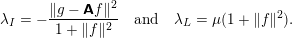 $$\begin{eqnarray}\unicode[STIX]{x1D706}_{I}=-\frac{\Vert g-\mathbf{\mathsf{A}}f\Vert ^{2}}{1+\Vert f\Vert ^{2}}\quad \text{and}\quad \unicode[STIX]{x1D706}_{L}=\unicode[STIX]{x1D707}(1+\Vert f\Vert ^{2}).\end{eqnarray}$$
In the above,
 $\unicode[STIX]{x1D707}$
is the Lagrange multiplier in
$\unicode[STIX]{x1D707}$
is the Lagrange multiplier in
 $$\begin{eqnarray}{\mathcal{L}}(\mathbf{\mathsf{\{}},f,\unicode[STIX]{x1D707})=\Vert \mathbf{\mathsf{\{}}f-g\Vert ^{2}+\Vert \mathbf{\mathsf{\{}}-\mathbf{\mathsf{A}}\Vert _{\text{F}}^{2}+\unicode[STIX]{x1D707}(\Vert \mathbf{\mathsf{L}}f\Vert ^{2}-\unicode[STIX]{x1D6FE}^{2}).\end{eqnarray}$$
The two parameters are related by
 $$\begin{eqnarray}\unicode[STIX]{x1D706}_{L}\unicode[STIX]{x1D6FE}^{2}=y^{\unicode[STIX]{x1D6FF},T}(g-\mathbf{\mathsf{A}}f)+\unicode[STIX]{x1D706}_{I}\end{eqnarray}$$
and the residual fulfils
 $$\begin{eqnarray}\Vert \mathbf{\mathsf{\{}}f-g\Vert ^{2}+\Vert \mathbf{\mathsf{\{}}-\mathbf{\mathsf{A}}\Vert _{\text{F}}^{2}=-\unicode[STIX]{x1D706}_{I}.\end{eqnarray}$$
Golub et al. (Reference Golub, Hansen and O’Leary1999) conclude that if
 $\Vert \mathbf{\mathsf{L}}f_{\unicode[STIX]{x1D6FE}}\Vert <\unicode[STIX]{x1D6FE}$
solves the R-TLS problem, then it also solves the TLS problem without regularization. Moreover, this approach has been extended to include sparsity constrained optimization (Zhu, Leus and Giannakis Reference Zhu, Leus and Giannakis2011), which equivalent formulation then reads
$\Vert \mathbf{\mathsf{L}}f_{\unicode[STIX]{x1D6FE}}\Vert <\unicode[STIX]{x1D6FE}$
solves the R-TLS problem, then it also solves the TLS problem without regularization. Moreover, this approach has been extended to include sparsity constrained optimization (Zhu, Leus and Giannakis Reference Zhu, Leus and Giannakis2011), which equivalent formulation then reads
The previous sparsity-promoting approach, as well as the original R-TLS approach, can be easily extended if sets of training data
 $(f_{i},g_{i})$
are available. One either aims for a two-stage approach to first update the operator and then solve the inverse problem with some new data point
$(f_{i},g_{i})$
are available. One either aims for a two-stage approach to first update the operator and then solve the inverse problem with some new data point
 $g$
, or one can integrate both steps at once leading to
$g$
, or one can integrate both steps at once leading to
Total least-squares is still an active field of research: see e.g. Markovsky and Van Huffel (Reference Markovsky and Van Huffel2007) and Beck, Sabach and Teboulle (Reference Beck, Sabach and Teboulle2016). Alternative problem formulations of the R-TLS problem in terms of given error bounds
 $\Vert y-g\Vert \leq \unicode[STIX]{x1D6FF}$
and
$\Vert y-g\Vert \leq \unicode[STIX]{x1D6FF}$
and
 $\Vert A-\tilde{A}\Vert \leq \unicode[STIX]{x1D716}$
(instead of
$\Vert A-\tilde{A}\Vert \leq \unicode[STIX]{x1D716}$
(instead of
 $\Vert \mathbf{\mathsf{L}}f\Vert \leq \unicode[STIX]{x1D6FE}$
as choosing an appropriate
$\Vert \mathbf{\mathsf{L}}f\Vert \leq \unicode[STIX]{x1D6FE}$
as choosing an appropriate
 $\unicode[STIX]{x1D6FE}$
can be challenging) were further investigated by Lu, Pereverzev and Tautenhahn (Reference Lu, Pereverzev and Tautenhahn2009) and Tautenhahn (Reference Tautenhahn2008). One further extension of the R-TLS is to include a regularization with respect to parameters determining the operator (operator deviation). This was considered in a general Hilbert space setting (Bleyer and Ramlau Reference Bleyer and Ramlau2013) for image deblurring (see Buccini, Donatelli and Ramlau Reference Buccini, Donatelli and Ramlau2018, who call it ‘semi-blind’).
$\unicode[STIX]{x1D6FE}$
can be challenging) were further investigated by Lu, Pereverzev and Tautenhahn (Reference Lu, Pereverzev and Tautenhahn2009) and Tautenhahn (Reference Tautenhahn2008). One further extension of the R-TLS is to include a regularization with respect to parameters determining the operator (operator deviation). This was considered in a general Hilbert space setting (Bleyer and Ramlau Reference Bleyer and Ramlau2013) for image deblurring (see Buccini, Donatelli and Ramlau Reference Buccini, Donatelli and Ramlau2018, who call it ‘semi-blind’).
For the purposes of the present review article we highlight the properties of TLS for applications in MPI: see Section 7.5, Knopp, Gdaniec and Möddel (Reference Knopp, Gdaniec and Möddel2017) and Kluth (Reference Kluth2018) for further information on MPI. The following is a brief summary of the results in Kluth and Maass (Reference Kluth and Maass2017). We seek to reconstruct a five-point phantom consisting of a glass capillary with a diameter of 1.1 mm filled with tracer with a concentration of 0.5 mol/l provided by the GitHub project page of Knopp et al. (Reference Knopp, Viereck, Bringout, Ahlborg, Rahmer and Hofmann2016). The data-driven reconstructions (obtained by using a measured noisy forward operator) are shown in Figure 6.1(a–d). We obtain smoothed reconstructions of the five points, which is typical for Tikhonov regularization: see Figure 6.1(a). In contrast, the minimization with sparsity constraints is able to obtain a better localization of the tracer. Signal energy from regions filled with tracer which are not included in the system matrix used may cause a larger concentration value than the expected 0.5 mol/l. Using the total least-squares approach further improves the localization in the sparse reconstruction for the data-based system matrices: see Figure 6.1(d).
A simplified model was fitted to measured data to obtain a knowledge-driven forward operator. As can be seen in Figure 6.1(e), using Tikhonov regularization results in a reconstruction of the five dots with additional background artefacts. Using the total least-squares approach in this set-up increases the contrast in concentration values but background artefacts are not significantly reduced. In contrast to the data-based reconstruction with Tikhonov regularization, the sparse knowledge-driven reconstruction in Figure 6.1(f) has a similar quality in terms of localization of the dots. By using the total least-squares approach, in Figure 6.1(h), the localization of the dots can be further improved such that the localization is similar in quality compared to the data-based sparse reconstruction.
Reconstructions of a five-point phantom (pixel size 1 mm) provided by Knopp et al. (Reference Knopp, Viereck, Bringout, Ahlborg, Rahmer and Hofmann2016) obtained using Tikhonov (with
 $\unicode[STIX]{x1D6FC}=0.1\times 10^{-6}$
) and sparsity-promoting (with
$\unicode[STIX]{x1D6FC}=0.1\times 10^{-6}$
) and sparsity-promoting (with
 $\unicode[STIX]{x1D6FC}=0.1$
) regularization with and without TLS. (a–d) Results from using a measured noisy forward operator. (e–h) Results from a knowledge-driven forward operator. Figure adapted from Kluth and Maass (Reference Kluth and Maass2017).
$\unicode[STIX]{x1D6FC}=0.1$
) regularization with and without TLS. (a–d) Results from using a measured noisy forward operator. (e–h) Results from a knowledge-driven forward operator. Figure adapted from Kluth and Maass (Reference Kluth and Maass2017).
6.2.3 Learned Landweber
Another approach to including a learning component into a forward operator is presented by Aspri, Banert, Öktem and Scherzer (Reference Aspri, Banert, Öktem and Scherzer2018). The starting point is to consider the iteratively regularized Landweber iteration (Scherzer Reference Scherzer1998) (see also Kaltenbacher et al. Reference Kaltenbacher, Neubauer and Scherzer2008), which amounts to computing the following iterative updates:
 $$\begin{eqnarray}f^{k+1}:=f^{k}-[\unicode[STIX]{x2202}{\mathcal{A}}(f^{k})]^{\ast }({\mathcal{A}}(f^{k})-g)-\unicode[STIX]{x1D706}_{k}(f^{k}-f^{0}),\end{eqnarray}$$
where
 $f^{0}\in X$
is an initial guess that incorporates a priori knowledge about the unknown
$f^{0}\in X$
is an initial guess that incorporates a priori knowledge about the unknown
 $f_{\text{true}}$
we seek. Next, one can introduce a data-driven damping factor in the above Landweber iteration:
$f_{\text{true}}$
we seek. Next, one can introduce a data-driven damping factor in the above Landweber iteration:
 $$\begin{eqnarray}f^{k+1}:=f^{k}-[\unicode[STIX]{x2202}{\mathcal{A}}(f^{k})]^{\ast }({\mathcal{A}}(f^{k})-g)-\unicode[STIX]{x1D706}_{k}[\unicode[STIX]{x2202}{\mathcal{B}}(f^{k})]^{\ast }({\mathcal{B}}(f^{k})-g).\end{eqnarray}$$
The (possibly non-linear) operator
 ${\mathcal{B}}:X\rightarrow Y$
can now be represented by a deep neural network that can be trained against supervised data by comparing the final iterate in (6.6) (iterates are stopped following the Morozov discrepancy principle (4.1)) against the ground truth for given data.
${\mathcal{B}}:X\rightarrow Y$
can now be represented by a deep neural network that can be trained against supervised data by comparing the final iterate in (6.6) (iterates are stopped following the Morozov discrepancy principle (4.1)) against the ground truth for given data.
Convergence and stability for the scheme in (6.6) in infinite-dimensional Hilbert spaces is proved by Aspri et al. (Reference Aspri, Banert, Öktem and Scherzer2018). This theoretical results are complemented by several numerical experiments for solving linear inverse problems for the Radon transform and a non-linear inverse problem of Schlieren tomography. In these examples, however, Aspri et al. (Reference Aspri, Banert, Öktem and Scherzer2018) restrict attention to a linear operator
 ${\mathcal{B}}$
.
${\mathcal{B}}$
.
6.3 Microlocal analysis
Microlocal analysis is a powerful mathematical theory for precisely describing how the singular part of a function, or more generally a distribution, is transformed under the action of an operator. Since its introduction to the mathematical community with the landmark publications by Sato (Reference Sato1971) and Hörmander (Reference Hörmander1971), it has proved itself useful in both pure and applied mathematical research. It is now a well-developed theory that can be used to study how singularities propagate under certain classes of operators, most notably Fourier integral operators, which include most differential and pseudo-differential operators as well as many integral operators frequently encountered in analysis, scientific computing and the physical sciences (Hörmander Reference Hörmander1971, Candès, Demanet and Ying Reference Candès, Demanet and Ying2007).
The crucial underlying observation in microlocal analysis is that the information about the location of the singularities (singular support) needs to be complemented by specifying those ‘directions’ along which singularities may propagate. Making this precise leads to the notion of the wavefront set of the function (or distribution).
Role in inverse problems.
Microlocal analysis is in particularly useful in inverse problems for a variety of reasons.
First, in many applications it is sufficient to recover the wavefront set of the model parameter from noisy data. For example, in imaging this would correspond to recovering the edges of the image from data. Such applications frequently arise when using imaging/sensing technologies where the transform is a pseudo-differential or Fourier integral operator (Krishnan and Quinto Reference Krishnan and Quinto2015). It turns out that one can use microlocal analysis to precisely describe how the wavefront set in data relates to the wavefront set for the model parameter, and this explicit relation is referred to as the (microlocal) canonical relation. Using the canonical relation one can recover the wavefront set from data without solving the inverse problem, a process that can be highly non-trivial.
Second, the canonical relation also describes which part of the wavefront set one can recover from data. This was done by Quinto (Reference Quinto1993) for the case when the two- or three-dimensional ray transform is restricted to parallel lines, and by Quinto and Öktem (Reference Quinto and Öktem2008) for an analysis in the region-of-interest limited angle setting. Faber, Katsevich and Ramm (Reference Faber, Katsevich and Ramm1995) derived a related principle for the three-dimensional ray transform restricted to lines given by helical acquisition, which is common in medical imaging. Similar principles hold for transforms integrating along other types of curves, e.g. ellipses with foci on the
 $x$
-axis and geodesics (Uhlmann and Vasy Reference Uhlmann and Vasy2012).
$x$
-axis and geodesics (Uhlmann and Vasy Reference Uhlmann and Vasy2012).
Finally, recovering the wavefront set of the model parameter from data is a less ill-posed procedure than attempting to recover the model parameter itself. This was demonstrated in Davison (Reference Davison1983), where the severely ill-posed reconstruction problem in limited angle CT becomes mildly ill-posed if one settles for recovering the wavefront. See also Quinto and Öktem (Reference Quinto and Öktem2008) for an application of this principle to cryo-electron tomography.
Data-driven extraction of the wavefront set.
The above motivates the inverse problems community to work with the wavefront set. One difficulty that has limited use of the wavefront set is that it is virtually impossible to extract it numerically from a digitized signal. This is due to its definition, which depends on the asymptotic behaviour of the Fourier transform after a localization procedure. An alternative possibility is to identify the wavefront set after transforming the signal using a suitable representation, e.g. a curvelet or shearlet transform (Candès and Donoho Reference Candès and Donoho2005, Kutyniok and Labate Reference Kutyniok and Labate2009). This requires analysing the rate of decay of transformed signal, which again is unfeasible in large-scale imaging applications.
A recent paper (Andrade-Loarca, Kutyniok, Öktem and Petersen Reference Andrade-Loarca, Kutyniok, Öktem and Petersen2019) uses a data-driven approach to training a wavefront set extractor applicable to noisy digitized signals. The idea is to construct a deep neural network classifier that predicts the wavefront set from the shearlet coefficients of a signal. The approach is successfully demonstrated on two-dimensional imaging examples where it outperforms all conventional edge-orientation estimators as well as alternative data-driven methods including the current state of the art. This learned wavefront set extractor can now be combined with a learned iterative method using the framework in Section 6.1.
Using the canonical relation to guide data-driven recovery.
In a recent paper Bubba et al. (Reference Bubba, Kutyniok, Lassas, März, Samek, Siltanen and Srinivasan2018) consider using the aforementioned microlocal canonical relation to steer a data-driven component in limited angle CT reconstruction, which is a severely ill-posed inverse problem.
Bubba et al. develop a hybrid reconstruction framework that fuses a knowledge-driven sparse regularization approach with a data-driven deep learning approach. The learning part is only applied to those parts that are not possible to recover (invisible part), which in turn can be characterized a priori through the canonical relation. The theoretically controllable sparse regularization is thus applied to the remaining parts that can be recovered (visible part).
This decomposition into visible and invisible parts is achieved numerically via the shearlet transform, which allows us to resolve wavefront sets in phase space. The neural network is then used to infer unknown shearlet coefficients associated with the invisible part.
7 Applications
In this section we revisit some of the machine learning methods for inverse problems discussed in the previous sections, and demonstrate their applicability to prototypical examples of inverse problems.
7.1 A simple example
We start the applications part of the paper by considering the exemplar inverse problem of ill-conditioned matrix inversion. This example should highlight the particular difficulties of applying learning to solve an ill-posed inverse problem. Surprisingly, even small
 $2\times 2$
examples cannot be solved reliably by straightforward neural networks! The results of this section are based on Maass (Reference Maass2019).
$2\times 2$
examples cannot be solved reliably by straightforward neural networks! The results of this section are based on Maass (Reference Maass2019).
This small-scale setting allows a somewhat complete analysis of the neural network; in particular, we can prove the shortcomings of such neural nets if the condition number of the matrix and the noise level in the data are in a critical relation. To be precise, in our most basic example we set
 $$\begin{eqnarray}{\mathcal{A}}_{\unicode[STIX]{x1D700}}(f)=\mathbf{\mathsf{A }}_{\unicode[STIX]{x1D700}}\cdot f\quad \text{where }\mathbf{\mathsf{A }}_{\unicode[STIX]{x1D700}}=\left(\begin{array}{@{}cc@{}}a_{11} & a_{12}\\ a_{21} & a_{22}\end{array}\right)=\left(\begin{array}{@{}cc@{}}1 & 1\\ 1 & 1+\unicode[STIX]{x1D700}\end{array}\right)\!.\end{eqnarray}$$
This matrix has eigenvalues
 $\unicode[STIX]{x1D706}_{1}=2+\unicode[STIX]{x1D700}/2+O(\unicode[STIX]{x1D700}^{2})$
and
$\unicode[STIX]{x1D706}_{1}=2+\unicode[STIX]{x1D700}/2+O(\unicode[STIX]{x1D700}^{2})$
and
 $\unicode[STIX]{x1D706}_{2}=\unicode[STIX]{x1D700}/2+O(\unicode[STIX]{x1D700}^{2})$
, with corresponding orthogonal eigenvectors
$\unicode[STIX]{x1D706}_{2}=\unicode[STIX]{x1D700}/2+O(\unicode[STIX]{x1D700}^{2})$
, with corresponding orthogonal eigenvectors
 $$\begin{eqnarray}u_{1}=\left(\begin{array}{@{}c@{}}1\\ 1\end{array}\right)+O(\unicode[STIX]{x1D700}^{2})\quad \text{and}\quad u_{2}=\left(\begin{array}{@{}c@{}}1\\ -1\end{array}\right)+O(\unicode[STIX]{x1D700}^{2}).\end{eqnarray}$$
The ill-posedness of the problem, or rather the condition number of
 $\mathbf{\mathsf{A}}_{\unicode[STIX]{x1D700}}$
, is controlled by
$\mathbf{\mathsf{A}}_{\unicode[STIX]{x1D700}}$
, is controlled by
 $1/\unicode[STIX]{x1D700}$
. Typical values we have in mind here are
$1/\unicode[STIX]{x1D700}$
. Typical values we have in mind here are
 $\unicode[STIX]{x1D700}=10^{-k}$
for
$\unicode[STIX]{x1D700}=10^{-k}$
for
 $k=0,\ldots ,10$
.
$k=0,\ldots ,10$
.
We now compare two methods for solving the inverse problem of recovering
 $f$
from
$f$
from
 $g=\mathbf{\mathsf{A}}_{\unicode[STIX]{x1D700}}\cdot f+e$
. The first is classical Tikhonov regularization, which only uses information about the operator
$g=\mathbf{\mathsf{A}}_{\unicode[STIX]{x1D700}}\cdot f+e$
. The first is classical Tikhonov regularization, which only uses information about the operator
 ${\mathcal{A}}_{\unicode[STIX]{x1D700}}$
. Here, given data
${\mathcal{A}}_{\unicode[STIX]{x1D700}}$
. Here, given data
 $g$
we estimate
$g$
we estimate
 $f_{\text{true}}$
by
$f_{\text{true}}$
by
 ${\mathcal{R}}_{\unicode[STIX]{x1D70E}}^{\text{Tik}}(g)$
, where
${\mathcal{R}}_{\unicode[STIX]{x1D70E}}^{\text{Tik}}(g)$
, where
 $$\begin{eqnarray}{\mathcal{R}}_{\unicode[STIX]{x1D70E}}^{\text{Tik}}(g):=({\mathcal{A}}_{\unicode[STIX]{x1D700}}^{\ast }\circ {\mathcal{A}}_{\unicode[STIX]{x1D700}}+\unicode[STIX]{x1D70E}^{2}\text{id})^{-1}\circ {\mathcal{A}}_{\unicode[STIX]{x1D700}}^{\ast }(g)=(\mathbf{\mathsf{A}}_{\unicode[STIX]{x1D700}}^{T}\cdot \mathbf{\mathsf{A}}_{\unicode[STIX]{x1D700}}+\unicode[STIX]{x1D70E}^{2}\mathbf{\mathsf{I}})^{-1}\cdot \mathbf{\mathsf{A}}_{\unicode[STIX]{x1D700}}^{T}\cdot g.\end{eqnarray}$$
The second inversion is based on a trained neural network, that is, given data
 $g$
we estimate
$g$
we estimate
 $f_{\text{true}}$
by
$f_{\text{true}}$
by
 ${\mathcal{R}}_{\mathbf{\mathsf{W}}^{\ast }}^{\text{NN}}(g)$
where
${\mathcal{R}}_{\mathbf{\mathsf{W}}^{\ast }}^{\text{NN}}(g)$
where
 ${\mathcal{R}}_{\mathbf{\mathsf{W}}^{\ast }}^{\text{NN}}:Y\rightarrow X$
is a trained neural network with
${\mathcal{R}}_{\mathbf{\mathsf{W}}^{\ast }}^{\text{NN}}:Y\rightarrow X$
is a trained neural network with
 $\mathbf{\mathsf{W}}^{\ast }$
given by
$\mathbf{\mathsf{W}}^{\ast }$
given by
In the above,
 $(f^{(i)},g^{(i)})\in X\times Y$
with
$(f^{(i)},g^{(i)})\in X\times Y$
with
 $i=1,\ldots ,m$
, where coefficients in
$i=1,\ldots ,m$
, where coefficients in
 $f^{(i)}$
are i.i.d. samples of a
$f^{(i)}$
are i.i.d. samples of a
 $N(0,1)$
distributed random variable, and
$N(0,1)$
distributed random variable, and
 $g^{(i)}:={\mathcal{A}}f^{(i)}+e^{(i)}$
, where
$g^{(i)}:={\mathcal{A}}f^{(i)}+e^{(i)}$
, where
 $e^{(i)}\in \mathbb{R}^{2}$
are i.i.d. samples of a
$e^{(i)}\in \mathbb{R}^{2}$
are i.i.d. samples of a
 $N(0,\unicode[STIX]{x1D70E}^{2})$
distributed random variable. This approach is fully data-driven and does not use any explicit knowledge about the operator
$N(0,\unicode[STIX]{x1D70E}^{2})$
distributed random variable. This approach is fully data-driven and does not use any explicit knowledge about the operator
 ${\mathcal{A}}$
.
${\mathcal{A}}$
.
Both methods are evaluated using a different set of test data and results are compared by computing the mean error:
 $$\begin{eqnarray}E^{\text{Tik}}:=\frac{1}{n}\mathop{\sum }_{i=1}^{n}\Vert {\mathcal{R}}_{\unicode[STIX]{x1D70E}}^{\text{Tik}}(g^{(i)})-f^{(i)}\Vert ^{2}\quad \text{and}\quad E^{\text{NN}}:=\frac{1}{n}\mathop{\sum }_{i=1}^{n}\Vert {\mathcal{R}}_{\mathbf{\mathsf{W}}}^{\text{NN}}(g^{(i)})-f^{(i)}\Vert ^{2},\end{eqnarray}$$
for
 $n$
test pairs
$n$
test pairs
 $(f^{(i)},g^{(i)})\in X\times Y$
with
$(f^{(i)},g^{(i)})\in X\times Y$
with
 $g^{(i)}:={\mathcal{A}}f^{(i)}+e^{(i)}$
as in the training set above but clearly distinct from the training examples.
$g^{(i)}:={\mathcal{A}}f^{(i)}+e^{(i)}$
as in the training set above but clearly distinct from the training examples.
The design of the network is crucial. We use a minimal network which allows us to reproduce a matrix vector multiplication. Hence the network is – in principle – capable of recovering the Tikhonov regularization operator or even an improvement of it. We use a network with a single hidden layer with four nodes. We restrict the eight weights connecting the two input variables with the first layer by setting
 $$\begin{eqnarray}\displaystyle & \displaystyle w_{1}=-w_{3}=w_{11},\quad w_{2}=-w_{4}=w_{12}, & \displaystyle \nonumber\\ \displaystyle & \displaystyle w_{5}=-w_{7}=w_{21},\quad w_{6}=-w_{8}=w_{22}, & \displaystyle \nonumber\end{eqnarray}$$
as depicted in Figure 7.1. We obtain a neural network depending on four variables
 $w_{11},w_{12},w_{21},w_{22}$
and the network acts as a multiplication of the matrix
$w_{11},w_{12},w_{21},w_{22}$
and the network acts as a multiplication of the matrix
 $$\begin{eqnarray}\mathbf{\mathsf{W}}=\left(\begin{array}{@{}cc@{}}w_{11} & w_{12}\\ w_{21} & w_{22}\end{array}\right)\end{eqnarray}$$
with the input vector
 $z=(z_{1},z_{2})$
. We denote the output of such a neural network by
$z=(z_{1},z_{2})$
. We denote the output of such a neural network by
 ${\mathcal{R}}_{\mathbf{\mathsf{W}}}^{\text{NN}}(z)=Wz$
.
${\mathcal{R}}_{\mathbf{\mathsf{W}}}^{\text{NN}}(z)=Wz$
.
The network design with eight parameters, a setting that yields a matrix–vector multiplication of the input.
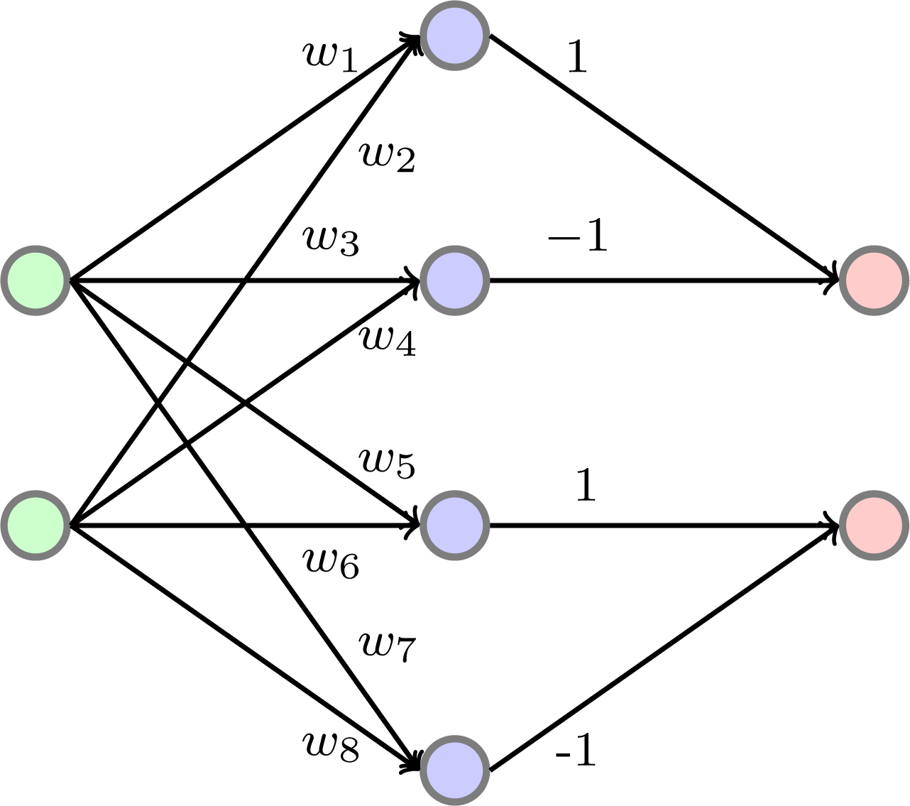
For later use we define
 $(2\times m)$
matrices
$(2\times m)$
matrices
 $\mathbf{\mathsf{X}},\mathbf{\mathsf{Y}}$
and
$\mathbf{\mathsf{X}},\mathbf{\mathsf{Y}}$
and
 $\mathbf{\mathsf{E}}$
that store the vectors
$\mathbf{\mathsf{E}}$
that store the vectors
 $f^{(i)},g^{(i)}$
and
$f^{(i)},g^{(i)}$
and
 $e^{(i)}$
column-wise, so the training data can be summarized as
$e^{(i)}$
column-wise, so the training data can be summarized as
 $$\begin{eqnarray}\mathbf{\mathsf{Y}}=\mathbf{\mathsf{A}}_{\unicode[STIX]{x1D700}}\cdot \mathbf{\mathsf{X}}+\mathbf{\mathsf{E}}.\end{eqnarray}$$
The training of such a network for modelling the forward problem is equivalent (using the Frobenius norm for matrices) to minimizing the expected mean square error
 $$\begin{eqnarray}\min _{\mathbf{\mathsf{W}}}~\frac{1}{n}\mathop{\sum }_{i=1}^{n}\Vert \mathbf{\mathsf{W}}f^{(i)}-g^{(i)}\Vert ^{2}=\min _{\mathbf{\mathsf{W}}}~\frac{1}{n}\Vert \mathbf{\mathsf{W}}\mathbf{\mathsf{X}}-\mathbf{\mathsf{Y}}\Vert ^{2},\end{eqnarray}$$
and the training model (7.2) for the inverse problem simplifies to
 $$\begin{eqnarray}\min _{\mathbf{\mathsf{W}}}~\frac{1}{n}\mathop{\sum }_{i=1}^{n}\Vert \mathbf{\mathsf{W}}g^{(i)}-f^{(i)}\Vert ^{2}=\min _{\mathbf{\mathsf{W}}}~\frac{1}{n}\Vert \mathbf{\mathsf{W}}\mathbf{\mathsf{Y}}-\mathbf{\mathsf{X}}\Vert ^{2}.\end{eqnarray}$$
In the next paragraph we report some numerical examples before analysing these networks.
Testing error convergence for various values of
$\unicode[STIX]{x1D700}$
.

We train these networks using a set of training data
 $(f^{(i)},g^{(i)})_{i=1,\ldots ,m}$
with
$(f^{(i)},g^{(i)})_{i=1,\ldots ,m}$
with
 $m=10\,000$
, i.e.
$m=10\,000$
, i.e.
 $g^{(i)}={\mathcal{A}}_{\unicode[STIX]{x1D700}}f^{(i)}+e^{(i)}$
. The network design with restricted coefficients as described above has four degrees of freedom
$g^{(i)}={\mathcal{A}}_{\unicode[STIX]{x1D700}}f^{(i)}+e^{(i)}$
. The network design with restricted coefficients as described above has four degrees of freedom
 $w=(w_{11},w_{12},w_{21},w_{22})$
. The corresponding loss function is minimized by a gradient descent algorithm, that is, the gradient of the loss function with respect to
$w=(w_{11},w_{12},w_{21},w_{22})$
. The corresponding loss function is minimized by a gradient descent algorithm, that is, the gradient of the loss function with respect to
 $w$
is computed by backpropagation (Rumelhart, Hinton and Williams Reference Rumelhart, Hinton, Williams, Rumelhart and McClelland1986, Martens and Sutskever Reference Martens and Sutskever2012, Byrd, Chin, Nocedal and Wu Reference Byrd, Chin, Nocedal and Wu2012). We used
$w$
is computed by backpropagation (Rumelhart, Hinton and Williams Reference Rumelhart, Hinton, Williams, Rumelhart and McClelland1986, Martens and Sutskever Reference Martens and Sutskever2012, Byrd, Chin, Nocedal and Wu Reference Byrd, Chin, Nocedal and Wu2012). We used
 $3000$
iterations (epochs) of this gradient descent to minimize the loss function of a network for the forward operator using (7.4) or, respectively, for training a network for solving the inverse problem using (7.2). The MSE errors on the training data were close to zero in both cases.
$3000$
iterations (epochs) of this gradient descent to minimize the loss function of a network for the forward operator using (7.4) or, respectively, for training a network for solving the inverse problem using (7.2). The MSE errors on the training data were close to zero in both cases.
After training we tested the resulting networks by drawing
 $n=10\,000$
new data vectors
$n=10\,000$
new data vectors
 $f^{(i)}$
as well as error vectors
$f^{(i)}$
as well as error vectors
 $e^{(i)}$
. The
$e^{(i)}$
. The
 $g^{(i)}$
were computed as above. Table 7.1 lists the resulting values using this set of test data for the network trained for the forward problem and the inverse problem, respectively:
$g^{(i)}$
were computed as above. Table 7.1 lists the resulting values using this set of test data for the network trained for the forward problem and the inverse problem, respectively:
 $$\begin{eqnarray}\displaystyle & \displaystyle \operatorname{NMSE}_{\text{fwd}}:=\frac{1}{n}\mathop{\sum }_{i=1}^{n}\Vert \mathbf{\mathsf{W}}f^{(i)}-g^{(i)}\Vert ^{2}, & \displaystyle \nonumber\\ \displaystyle & \displaystyle \operatorname{NMSE}_{\text{inv}}:=\frac{1}{n}\mathop{\sum }_{i=1}^{n}\Vert \mathbf{\mathsf{W}}f^{(i)}-g^{(i)}\Vert ^{2}. & \displaystyle \nonumber\end{eqnarray}$$
The errors of the inverse net with an ill-conditioned matrix
 $\mathbf{\mathsf{A}}_{\unicode[STIX]{x1D700}}$
(i.e.
$\mathbf{\mathsf{A}}_{\unicode[STIX]{x1D700}}$
(i.e.
 $\unicode[STIX]{x1D700}\!\ll \!1$
) are large and the computed reconstructions with the test data are meaningless.
$\unicode[STIX]{x1D700}\!\ll \!1$
) are large and the computed reconstructions with the test data are meaningless.
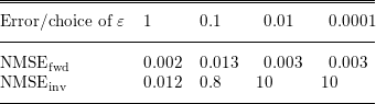
We observe that training the forward operator produces reliable results, as does the network for the inverse problem with
 $\unicode[STIX]{x1D700}\geq 0.1$
. However, training a network for the inverse problem with an ill-conditioned matrix
$\unicode[STIX]{x1D700}\geq 0.1$
. However, training a network for the inverse problem with an ill-conditioned matrix
 $\mathbf{\mathsf{A}}_{\unicode[STIX]{x1D700}}$
with
$\mathbf{\mathsf{A}}_{\unicode[STIX]{x1D700}}$
with
 $\unicode[STIX]{x1D700}\leq 0.01$
fails. This is confirmed by analysing the values of
$\unicode[STIX]{x1D700}\leq 0.01$
fails. This is confirmed by analysing the values of
 $w$
and of the resulting matrix
$w$
and of the resulting matrix
 $\mathbf{\mathsf{W}}$
after training. We would expect that in training the forward problem will produce values for
$\mathbf{\mathsf{W}}$
after training. We would expect that in training the forward problem will produce values for
 $\mathbf{\mathsf{W}}$
such that
$\mathbf{\mathsf{W}}$
such that
 $\mathbf{\mathsf{W}}\sim \mathbf{\mathsf{A}}_{\unicode[STIX]{x1D700}}$
and that training the inverse problems leads to
$\mathbf{\mathsf{W}}\sim \mathbf{\mathsf{A}}_{\unicode[STIX]{x1D700}}$
and that training the inverse problems leads to
 $\mathbf{\mathsf{W}}\sim {\mathcal{R}}_{\unicode[STIX]{x1D70E}}^{\text{Tik}}(g)$
for some regularization parameter
$\mathbf{\mathsf{W}}\sim {\mathcal{R}}_{\unicode[STIX]{x1D70E}}^{\text{Tik}}(g)$
for some regularization parameter
 $\unicode[STIX]{x1D70E}$
. For the forward problem, the difference between
$\unicode[STIX]{x1D70E}$
. For the forward problem, the difference between
 $\mathbf{\mathsf{W}}$
and
$\mathbf{\mathsf{W}}$
and
 $\mathbf{\mathsf{A}}_{\unicode[STIX]{x1D700}}$
is of order
$\mathbf{\mathsf{A}}_{\unicode[STIX]{x1D700}}$
is of order
 $10^{-3}$
or below, but for
$10^{-3}$
or below, but for
 $\unicode[STIX]{x1D700}\leq 0.01$
the training of the inverse problem leads to a matrix that has no similarity to the Tikhonov regularized inverse. Using a network with a single internal layer but with more nodes and no restriction on the structure of the weights did not yield any significant improvements.
$\unicode[STIX]{x1D700}\leq 0.01$
the training of the inverse problem leads to a matrix that has no similarity to the Tikhonov regularized inverse. Using a network with a single internal layer but with more nodes and no restriction on the structure of the weights did not yield any significant improvements.
Analysis of trivial neural networks for inverse problems.
In this section we analyse the case where the application of the neural network is strictly equivalent to a matrix–vector multiplication, that is, training of the network is given by (7.5). The optimal
 $\mathbf{\mathsf{W}}$
in (7.5) is given by
$\mathbf{\mathsf{W}}$
in (7.5) is given by
 $$\begin{eqnarray}\mathbf{\mathsf{W}}^{T}=(\mathbf{\mathsf{Y}}\mathbf{\mathsf{Y}}^{T})^{-1}\mathbf{\mathsf{Y}}\mathbf{\mathsf{X}}^{T}.\end{eqnarray}$$
Standard arguments show that, together with that hypothesized in the numerical discussion above, the
 $\mathbf{\mathsf{W}}$
in (7.6) coincides with the Tikhonov regularizers
$\mathbf{\mathsf{W}}$
in (7.6) coincides with the Tikhonov regularizers
 ${\mathcal{R}}_{\unicode[STIX]{x1D70E}}^{\text{Tik}}(g)$
from (7.1). This is not a surprising result since (7.6) coincides with the classical maximum a posteriori (MAP) estimator of statistical inverse problems. However, analysing the variance
${\mathcal{R}}_{\unicode[STIX]{x1D70E}}^{\text{Tik}}(g)$
from (7.1). This is not a surprising result since (7.6) coincides with the classical maximum a posteriori (MAP) estimator of statistical inverse problems. However, analysing the variance
 $\mathbb{E}[\Vert \mathbf{\mathsf{W}}-\mathbf{\mathsf{T}}\Vert ^{2}]$
, where
$\mathbb{E}[\Vert \mathbf{\mathsf{W}}-\mathbf{\mathsf{T}}\Vert ^{2}]$
, where
 $\mathbf{\mathsf{T}}=(\mathbf{\mathsf{A}}_{\unicode[STIX]{x1D700}}^{T}\cdot \mathbf{\mathsf{A}}_{\unicode[STIX]{x1D700}}+\unicode[STIX]{x1D70E}^{2}\mathbf{\mathsf{I}})^{-1}\cdot \mathbf{\mathsf{A}}_{\unicode[STIX]{x1D700}}^{T}$
is the Tikhonov reconstruction matrix, reflects the ill-posedness of the problem. Indeed, as is demonstrated in a series of numerical tests in Maass (Reference Maass2019), the deviation of
$\mathbf{\mathsf{T}}=(\mathbf{\mathsf{A}}_{\unicode[STIX]{x1D700}}^{T}\cdot \mathbf{\mathsf{A}}_{\unicode[STIX]{x1D700}}+\unicode[STIX]{x1D70E}^{2}\mathbf{\mathsf{I}})^{-1}\cdot \mathbf{\mathsf{A}}_{\unicode[STIX]{x1D700}}^{T}$
is the Tikhonov reconstruction matrix, reflects the ill-posedness of the problem. Indeed, as is demonstrated in a series of numerical tests in Maass (Reference Maass2019), the deviation of
 $\mathbf{\mathsf{W}}$
from
$\mathbf{\mathsf{W}}$
from
 $\mathbf{\mathsf{T}}$
will be arbitrarily large if
$\mathbf{\mathsf{T}}$
will be arbitrarily large if
 $\unicode[STIX]{x1D700}$
and
$\unicode[STIX]{x1D700}$
and
 $\unicode[STIX]{x1D70E}$
are both small. Of course, we can also give this a positive meaning: the noise level acts as a regularizer, and large
$\unicode[STIX]{x1D70E}$
are both small. Of course, we can also give this a positive meaning: the noise level acts as a regularizer, and large
 $\unicode[STIX]{x1D70E}$
yields more stable matrices
$\unicode[STIX]{x1D70E}$
yields more stable matrices
 $\mathbf{\mathsf{W}}$
. See Maass (Reference Maass2019) for details.
$\mathbf{\mathsf{W}}$
. See Maass (Reference Maass2019) for details.
This small example clearly illustrates that one needs to have some insight into the nature of inverse problems for successfully applying deep learning techniques. Performance of practical examples of more targeted deep learning approaches to inverse problems will be discussed in the following Sections 7.3, 7.4, 7.6 and 7.7.
(a–c) Effect of choosing
 $\unicode[STIX]{x1D6FD}$
on TGV
$\unicode[STIX]{x1D6FD}$
on TGV
 $^{2}$
denoising with optimal
$^{2}$
denoising with optimal
 $\unicode[STIX]{x1D6FC}$
. (d–f) Effect of choosing
$\unicode[STIX]{x1D6FC}$
. (d–f) Effect of choosing
 $\unicode[STIX]{x1D6FC}$
too large in TGV
$\unicode[STIX]{x1D6FC}$
too large in TGV
 $^{2}$
denoising.
$^{2}$
denoising.
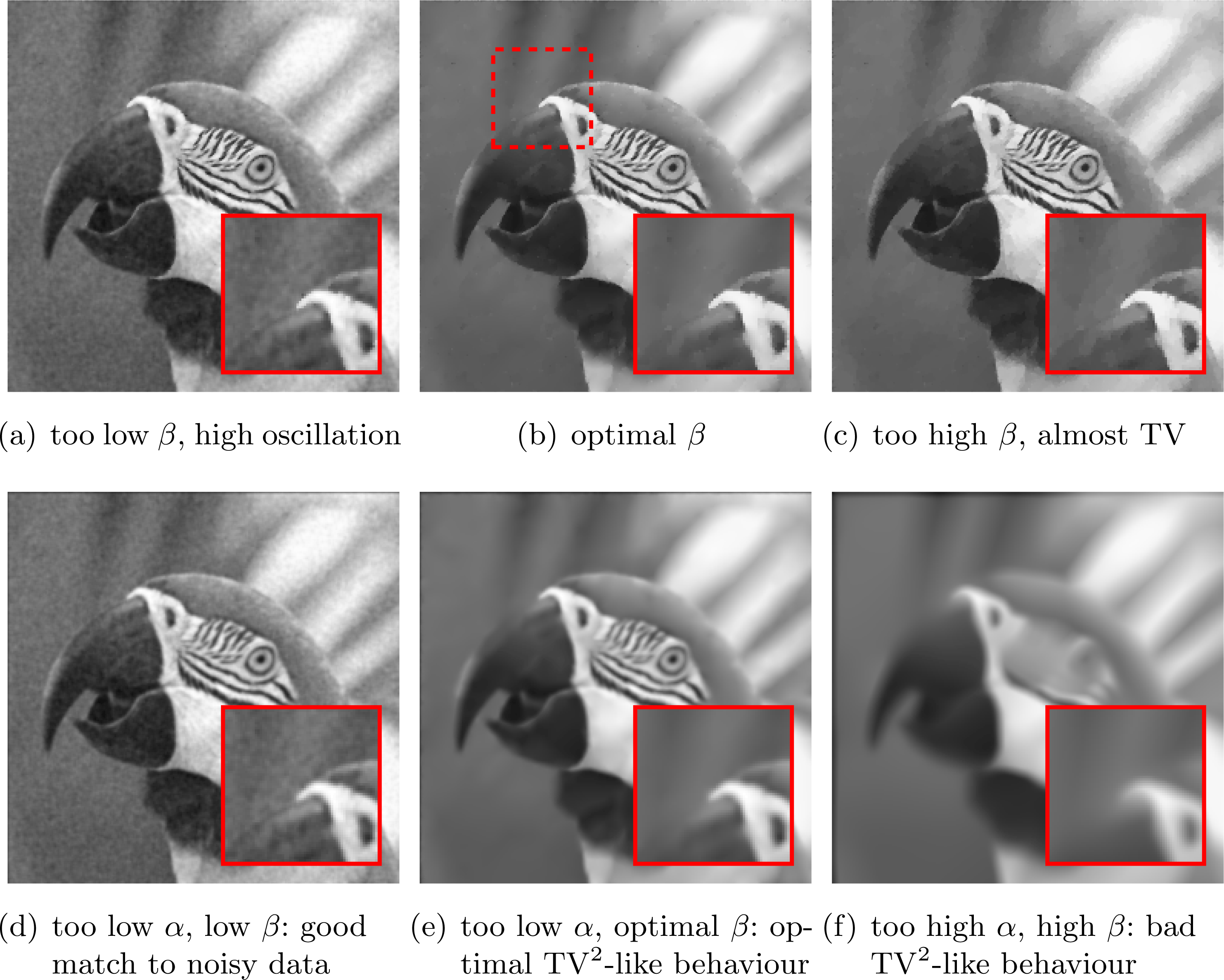
7.2 Bilevel learning for TV image denoising
In (4.4) bilevel learning of TV-type regularizers was discussed as a way to make functional analytic regularization more data-driven. In what follows, we showcase some results of this learning approach for the case of image denoising, i.e.
 ${\mathcal{A}}=\text{id}$
.
${\mathcal{A}}=\text{id}$
.
Optimal TV-regularizers for image denoising.
The regularization effect of TV and second-order TV approaches heavily depends on the choice of regularization parameters
 $\unicode[STIX]{x1D703}=\unicode[STIX]{x1D6FC}$
(i.e.
$\unicode[STIX]{x1D703}=\unicode[STIX]{x1D6FC}$
(i.e.
 $=(\unicode[STIX]{x1D6FC},\unicode[STIX]{x1D6FD})$
for second-order TV approaches). In Figure 7.2 we show the effect of different choices of
$=(\unicode[STIX]{x1D6FC},\unicode[STIX]{x1D6FD})$
for second-order TV approaches). In Figure 7.2 we show the effect of different choices of
 $\unicode[STIX]{x1D6FC}$
and
$\unicode[STIX]{x1D6FC}$
and
 $\unicode[STIX]{x1D6FD}$
in
$\unicode[STIX]{x1D6FD}$
in
 $\operatorname{TGV}^{2}$
denoising. In what follows we show some results from De los Reyes et al. (Reference De los Reyes, Schönlieb and Valkonen2017) applying the learning approach from (4.4) with the smoothed regularizer (4.6) to find optimal parameters in TV-type reconstruction models. The regularization effect of TV and second-order TV approaches heavily depends on the choice of regularization parameters
$\operatorname{TGV}^{2}$
denoising. In what follows we show some results from De los Reyes et al. (Reference De los Reyes, Schönlieb and Valkonen2017) applying the learning approach from (4.4) with the smoothed regularizer (4.6) to find optimal parameters in TV-type reconstruction models. The regularization effect of TV and second-order TV approaches heavily depends on the choice of regularization parameters
 $\unicode[STIX]{x1D703}=\unicode[STIX]{x1D6FC}$
(i.e.
$\unicode[STIX]{x1D703}=\unicode[STIX]{x1D6FC}$
(i.e.
 $=(\unicode[STIX]{x1D6FC},\unicode[STIX]{x1D6FD})$
for second-order TV approaches).
$=(\unicode[STIX]{x1D6FC},\unicode[STIX]{x1D6FD})$
for second-order TV approaches).
Contour plot of the objective functional in
 $\operatorname{TGV}^{2}$
denoising in the
$\operatorname{TGV}^{2}$
denoising in the
 $(\unicode[STIX]{x1D6FC},\unicode[STIX]{x1D6FD})$
-plane.
$(\unicode[STIX]{x1D6FC},\unicode[STIX]{x1D6FD})$
-plane.
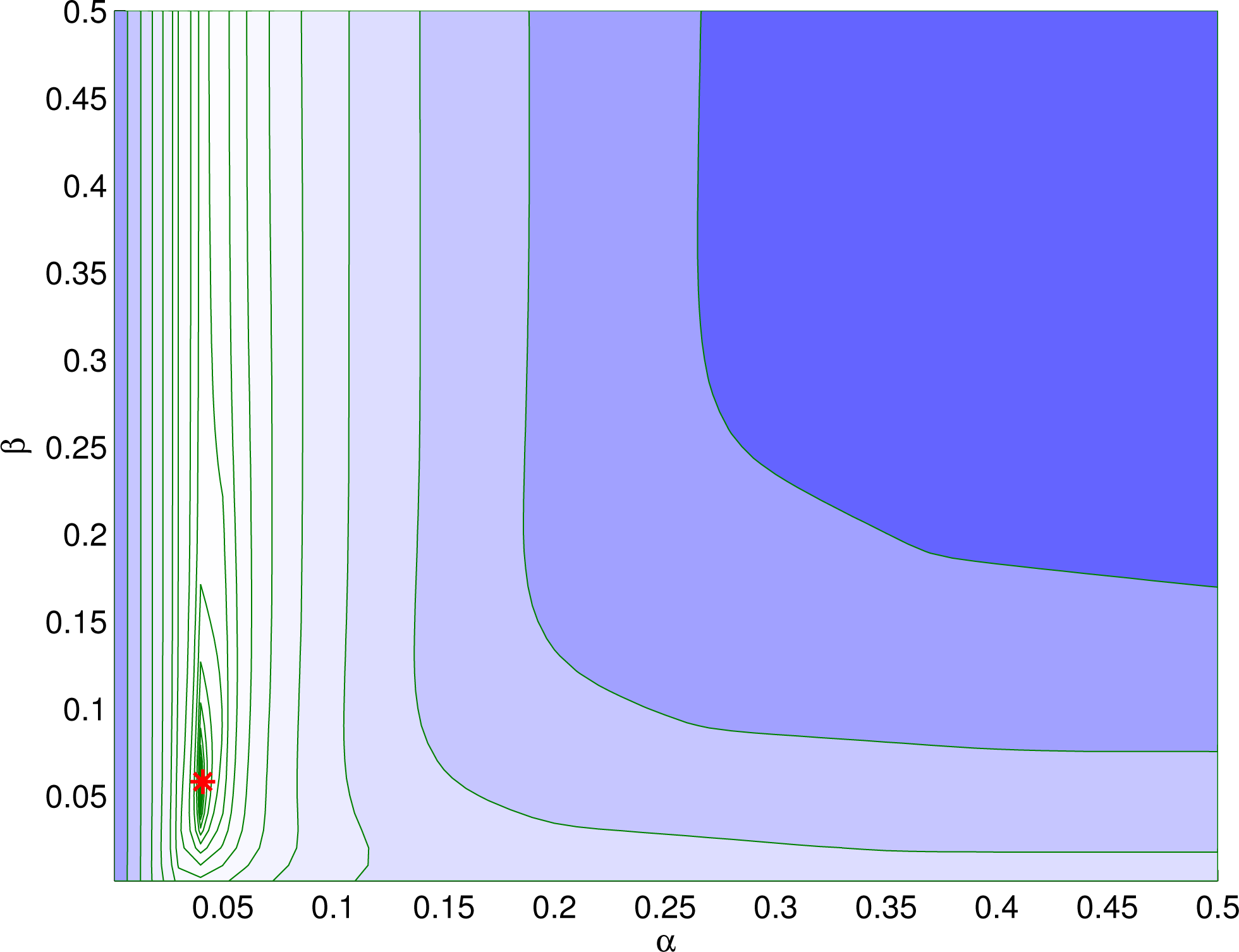
Optimal denoising results for
 $\operatorname{TGV}^{2}$
,
$\operatorname{TGV}^{2}$
,
 $\operatorname{ICTV}$
and TV, all with
$\operatorname{ICTV}$
and TV, all with
 $L_{2}^{2}$
as data discrepancy.
$L_{2}^{2}$
as data discrepancy.
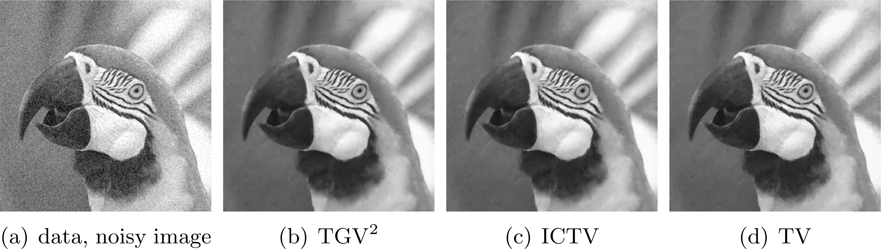
Quantified results for the parrot image (
 $s:=$
image width/height in pixels
$s:=$
image width/height in pixels
 $\,=256$
), using
$\,=256$
), using
 $L_{2}^{2}$
discrepancy.
$L_{2}^{2}$
discrepancy.
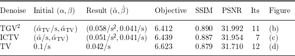
The first example is TGV denoising of an image corrupted with white Gaussian noise with PSNR of
 $24.72$
. The red dot in Figure 7.3 plots the discovered regularization parameter
$24.72$
. The red dot in Figure 7.3 plots the discovered regularization parameter
 $\widehat{\unicode[STIX]{x1D703}}=(\hat{\unicode[STIX]{x1D6FC}},\hat{\unicode[STIX]{x1D6FD}})$
reported in Figure 7.4. Studying the location of the red dot, we may conclude that the Broyden–Fletcher–Goldfarb–Shanno (BFGS) algorithm managed to find a nearly optimal parameter in very few iterations: see Table 7.2. Although the optimization problem for
$\widehat{\unicode[STIX]{x1D703}}=(\hat{\unicode[STIX]{x1D6FC}},\hat{\unicode[STIX]{x1D6FD}})$
reported in Figure 7.4. Studying the location of the red dot, we may conclude that the Broyden–Fletcher–Goldfarb–Shanno (BFGS) algorithm managed to find a nearly optimal parameter in very few iterations: see Table 7.2. Although the optimization problem for
 $(\unicode[STIX]{x1D6FC},\unicode[STIX]{x1D6FD})$
is non-convex, in all of our experiments we observed commendable convergence behaviour of the BFGS algorithm: see De los Reyes et al. (Reference De los Reyes, Schönlieb and Valkonen2017) for further examples.
$(\unicode[STIX]{x1D6FC},\unicode[STIX]{x1D6FD})$
is non-convex, in all of our experiments we observed commendable convergence behaviour of the BFGS algorithm: see De los Reyes et al. (Reference De los Reyes, Schönlieb and Valkonen2017) for further examples.
To test the generalization quality of the bilevel learning model in De los Reyes et al. (Reference De los Reyes, Schönlieb and Valkonen2017), optimal parameters were cross-validated when tested for image denoising on the Berkeley segmentation data set (BSDS300) (Martin, Fowlkes, Tal and Malik Reference Martin, Fowlkes, Tal and Malik2001). A dataset of 200 images was selected and split into two halves of 100 images each. Optimal parameters were learned for each half individually, and then used to denoise the images of the other half. The results for TV denoising with
 $L^{2}$
-loss function and data fidelity are reported in Table 7.3. The results for TGV denoising are reported in Table 7.4. In both experiments the parameters seem to be robust against cross-validation, both in terms of their optimal value, and average PSNR and SSIM (Wang, Bovik, Sheikh and Simoncelli Reference Wang, Bovik, Sheikh and Simoncelli2004) quality measures of the denoised image.
$L^{2}$
-loss function and data fidelity are reported in Table 7.3. The results for TGV denoising are reported in Table 7.4. In both experiments the parameters seem to be robust against cross-validation, both in terms of their optimal value, and average PSNR and SSIM (Wang, Bovik, Sheikh and Simoncelli Reference Wang, Bovik, Sheikh and Simoncelli2004) quality measures of the denoised image.
Cross-validated computations on the BSDS300 data set (Martin et al.
Reference Martin, Fowlkes, Tal and Malik2001) split into two halves of 100 images each. TV regularization with
 $L^{2}$
-discrepancy and fidelity function. ‘Learning’ and ‘validation’ indicate the halves used for learning
$L^{2}$
-discrepancy and fidelity function. ‘Learning’ and ‘validation’ indicate the halves used for learning
 $\unicode[STIX]{x1D6FC}$
and for computing the average PSNR and SSIM, respectively. Noise variance
$\unicode[STIX]{x1D6FC}$
and for computing the average PSNR and SSIM, respectively. Noise variance
 $\unicode[STIX]{x1D70E}=10$
.
$\unicode[STIX]{x1D70E}=10$
.
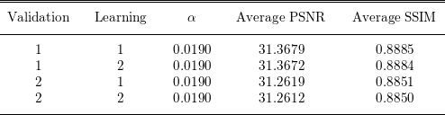
Cross-validated computations on the BSDS300 data set (Martin et al.
Reference Martin, Fowlkes, Tal and Malik2001) split into two halves of 100 images each.
 $\operatorname{TGV}^{2}$
regularization with
$\operatorname{TGV}^{2}$
regularization with
 $L^{2}$
-discrepancy. ‘Learning’ and ‘validation’ indicate the halves used for learning
$L^{2}$
-discrepancy. ‘Learning’ and ‘validation’ indicate the halves used for learning
 $\unicode[STIX]{x1D6FC}$
and for computing the average PSNR and SSIM, respectively. Noise variance
$\unicode[STIX]{x1D6FC}$
and for computing the average PSNR and SSIM, respectively. Noise variance
 $\unicode[STIX]{x1D70E}=10$
.
$\unicode[STIX]{x1D70E}=10$
.
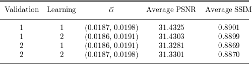
Bilevel learning of the data discrepancy term in mixed noise scenarios.
In the examples in the previous paragraph we considered bilevel parameter learning for TV-type image denoising, assuming that the noise in the image is normally distributed and consequently an
 $L^{2}$
-data discrepancy term is the appropriate choice to take. The bilevel learning model (4.4), however, is capable of linear combinations of data discrepancy terms as in (4.5) which might be appropriate in situations of multiple noise distributions in the data: see e.g. Lanza, Morigi, Sgallari and Wen (Reference Lanza, Morigi, Sgallari and Wen2014), De los Reyes and Schönlieb (Reference De los Reyes and Schönlieb2013), Calatroni et al. (Reference Calatroni, De los Reyes and Schönlieb2017) and Calatroni (Reference Calatroni2015) and references therein. Calatroni et al. (Reference Calatroni, De los Reyes and Schönlieb2017) also considered infimal convolutions of data discrepancy functions.
$L^{2}$
-data discrepancy term is the appropriate choice to take. The bilevel learning model (4.4), however, is capable of linear combinations of data discrepancy terms as in (4.5) which might be appropriate in situations of multiple noise distributions in the data: see e.g. Lanza, Morigi, Sgallari and Wen (Reference Lanza, Morigi, Sgallari and Wen2014), De los Reyes and Schönlieb (Reference De los Reyes and Schönlieb2013), Calatroni et al. (Reference Calatroni, De los Reyes and Schönlieb2017) and Calatroni (Reference Calatroni2015) and references therein. Calatroni et al. (Reference Calatroni, De los Reyes and Schönlieb2017) also considered infimal convolutions of data discrepancy functions.
Figures 7.5 and 7.6 present denoising results with optimally learned parameters for mixed Gaussian and impulse noise and for mixed Gaussian and Poisson noise, respectively. See Calatroni et al. (Reference Calatroni, De los Reyes and Schönlieb2017) for more details. The original image has been corrupted with Gaussian noise of zero mean and variance
 $0.005$
and then a percentage of
$0.005$
and then a percentage of
 $5\%$
of pixels has been corrupted with impulse noise. The parameters have been chosen to be
$5\%$
of pixels has been corrupted with impulse noise. The parameters have been chosen to be
 $\unicode[STIX]{x1D6FE}=10^{4}$
,
$\unicode[STIX]{x1D6FE}=10^{4}$
,
 $\unicode[STIX]{x1D707}=10^{-15}$
and the mesh step size
$\unicode[STIX]{x1D707}=10^{-15}$
and the mesh step size
 $h=1/312$
. The computed optimal weights are
$h=1/312$
. The computed optimal weights are
 $\hat{\unicode[STIX]{x1D706}}_{1}=734.25$
and
$\hat{\unicode[STIX]{x1D706}}_{1}=734.25$
and
 $\hat{\unicode[STIX]{x1D706}}_{2}=3401.2$
. Together with an optimal denoised image, the results show the decomposition of the noise into its sparse and Gaussian components: see Calatroni et al. (Reference Calatroni, De los Reyes and Schönlieb2017) for more details.
$\hat{\unicode[STIX]{x1D706}}_{2}=3401.2$
. Together with an optimal denoised image, the results show the decomposition of the noise into its sparse and Gaussian components: see Calatroni et al. (Reference Calatroni, De los Reyes and Schönlieb2017) for more details.
Optimized impulse-Gaussian denoising: (a) original image, (b) noisy image with Gaussian noise of variance
 $0.005$
and (c) with
$0.005$
and (c) with
 $5\%$
of pixels corrupted with impulse noise, (d) impulse noise residuum, (e) Gaussian noise residuum. Optimal parameters
$5\%$
of pixels corrupted with impulse noise, (d) impulse noise residuum, (e) Gaussian noise residuum. Optimal parameters
 $\hat{\unicode[STIX]{x1D706}}_{1}=734.25$
and
$\hat{\unicode[STIX]{x1D706}}_{1}=734.25$
and
 $\hat{\unicode[STIX]{x1D706}}_{2}=3401.2$
.
$\hat{\unicode[STIX]{x1D706}}_{2}=3401.2$
.
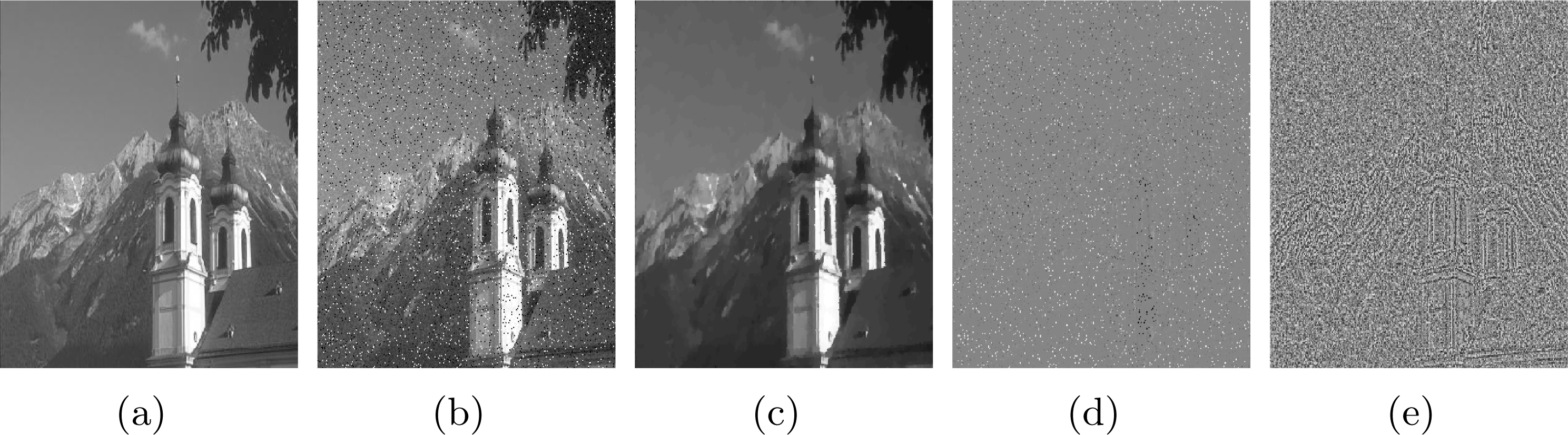
Optimized Poisson–Gauss denoising: (a) original image, (b) noisy image corrupted by Poisson noise and Gaussian noise with mean zero and variance
 $0.001$
, (c) denoised image. Optimal parameters
$0.001$
, (c) denoised image. Optimal parameters
 $\hat{\unicode[STIX]{x1D706}}_{1}=1847.75$
and
$\hat{\unicode[STIX]{x1D706}}_{1}=1847.75$
and
 $\hat{\unicode[STIX]{x1D706}}_{2}=73.45$
.
$\hat{\unicode[STIX]{x1D706}}_{2}=73.45$
.
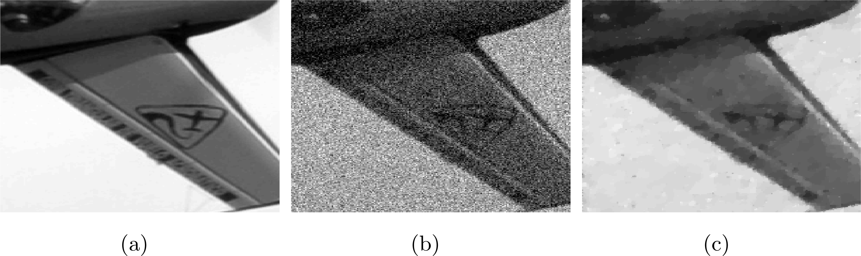
Remark 7.1. When optimizing only a handful of scalar parameters, as in the examples discussed above, bilevel optimization is by no means the most efficient approach for parameter learning. In fact, brute force line-search methods are in this context still computationally feasible as the dimensionality of the parameter space being explored is small. However, even in this small parameter example, investigating bilevel optimization methods is instructive, as it tells us something about the mathematical properties of parameter learning for the typically considered non-smooth variational regularization problems and the numerical approaches with which they can be tackled. Insight gained from this becomes particularly important when going to more advanced parametrizations, for instance when optimizing spatially varying regularization parameters (Van Chung et al. Reference Van Chung, De los Reyes and Schönlieb2017) or different discrete parametrizations, as considered in Sections 4.3.2, 4.4 or 4.7.
7.3 Learned iterative reconstruction for computed tomography (CT) and photoacoustic tomography (PAT)
Learned iterative reconstruction schemes (Section 5.1.4) have been successfully applied to several large-scale inverse problems in imaging, such as image reconstruction in MRI, CT and PAT. We will show examples from CT taken from Adler and Öktem (Reference Adler and Öktem2017, Reference Adler and Öktem2018b ) and PAT taken from Hauptmann et al. (Reference Hauptmann, Lucka, Betcke, Huynh, Adler, Cox, Beard, Ourselin and Arridge2018).
7.3.1 CT image reconstruction
The learned primal–dual scheme in Adler and Öktem (Reference Adler and Öktem2018b ) is here tested on the two-dimensional CT image reconstruction problem, and its performance is evaluated in a simplified setting as well as a more realistic setting.
The forward operator for pre-log data is expressible in terms of the ray transform of (2.5), and for log data it is given by the ray transform of (2.6). The model parameter is a real-valued function defined on a domain
 $\unicode[STIX]{x1D6FA}\subset \mathbb{R}^{2}$
. This function represents the image we seek to recover and we assume
$\unicode[STIX]{x1D6FA}\subset \mathbb{R}^{2}$
. This function represents the image we seek to recover and we assume
 $X\subset L^{2}(\unicode[STIX]{x1D6FA})$
is a suitable vector space of such functions.
$X\subset L^{2}(\unicode[STIX]{x1D6FA})$
is a suitable vector space of such functions.
This data set is used to train both the learned post-processing and learned iterative methods, where the former is filtered back projection (FBP) reconstruction followed by a trained denoiser with a U-Net architecture and the latter is the learned primal–dual method in Adler and Öktem (Reference Adler and Öktem2018b
). Both networks were trained using the squared
 $L^{2}$
-loss. The other two knowledge-driven reconstruction methods are the standard FBP and (isotropic) TV-regularized reconstruction. The FBP reconstructions is applied to log data using a Hann filter; the TV reconstruction was solved using 1000 iterations of the classical primal–dual hybrid gradient algorithm. The filter bandwidth in the FBP and the regularization parameter in the TV reconstruction were selected in order to maximize the PSNR.
$L^{2}$
-loss. The other two knowledge-driven reconstruction methods are the standard FBP and (isotropic) TV-regularized reconstruction. The FBP reconstructions is applied to log data using a Hann filter; the TV reconstruction was solved using 1000 iterations of the classical primal–dual hybrid gradient algorithm. The filter bandwidth in the FBP and the regularization parameter in the TV reconstruction were selected in order to maximize the PSNR.
In the simplified setting shown in Figure 7.8 (see also the summary in Table 7.5) the images are
 $128\times 128$
pixel step functions, and we use supervised training data consisting of about 50 000 pairs of images and corresponding data as in Figure 7.7. Noise is 5% additive Gaussian. The images in the training data are randomly generated using a known probability distribution, and corresponding tomographic data (sinogram) are simulated with 5% additive Gaussian noise. This is a relatively small-scale problem, which allows us to also compute the conditional mean reconstruction using MCMC techniques (Section 3.5.2). The conditional mean reconstruction is useful since the learned iterative method approximates it. The same holds for learned post-processing since FBP is a linear sufficient statistic: see the discussion in Section 5.1.5. Hence, neither learned post-processing nor learned iterative will outperform the conditional mean, irrespective of the amount of training data and model capacity, that is, the conditional mean reconstruction serves as a theoretical limit for what one can recover.
$128\times 128$
pixel step functions, and we use supervised training data consisting of about 50 000 pairs of images and corresponding data as in Figure 7.7. Noise is 5% additive Gaussian. The images in the training data are randomly generated using a known probability distribution, and corresponding tomographic data (sinogram) are simulated with 5% additive Gaussian noise. This is a relatively small-scale problem, which allows us to also compute the conditional mean reconstruction using MCMC techniques (Section 3.5.2). The conditional mean reconstruction is useful since the learned iterative method approximates it. The same holds for learned post-processing since FBP is a linear sufficient statistic: see the discussion in Section 5.1.5. Hence, neither learned post-processing nor learned iterative will outperform the conditional mean, irrespective of the amount of training data and model capacity, that is, the conditional mean reconstruction serves as a theoretical limit for what one can recover.
Example from supervised training data used to train the learned iterative and learned post-processing methods used in Figure 7.8.
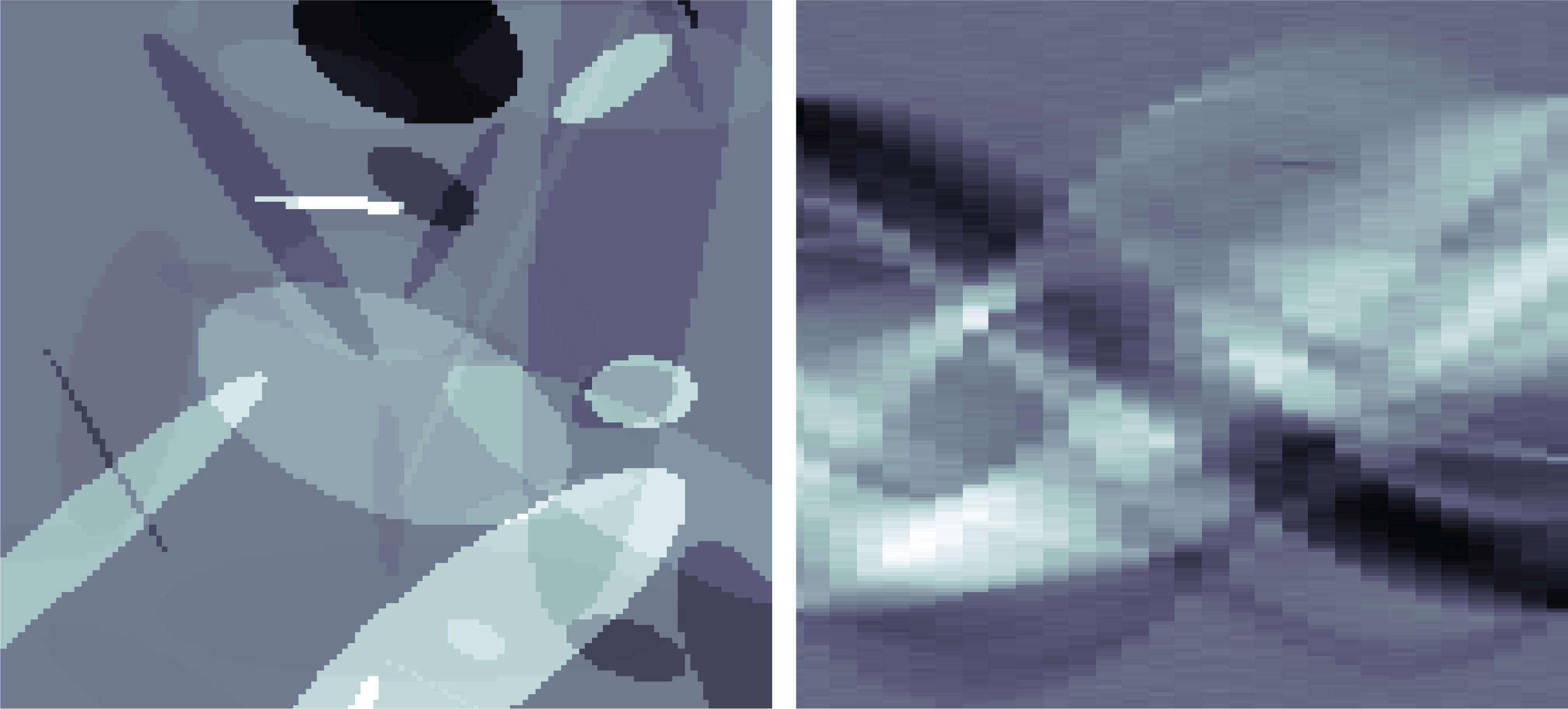
Reconstructions of the Shepp–Logan phantom using different methods. The window is set to
 $[0.1,0.4]$
, corresponding to the soft tissue of the modified Shepp–Logan phantom. We can see that the learned iterative method does indeed approximate the Bayes estimator, which here equals the conditional mean.
$[0.1,0.4]$
, corresponding to the soft tissue of the modified Shepp–Logan phantom. We can see that the learned iterative method does indeed approximate the Bayes estimator, which here equals the conditional mean.
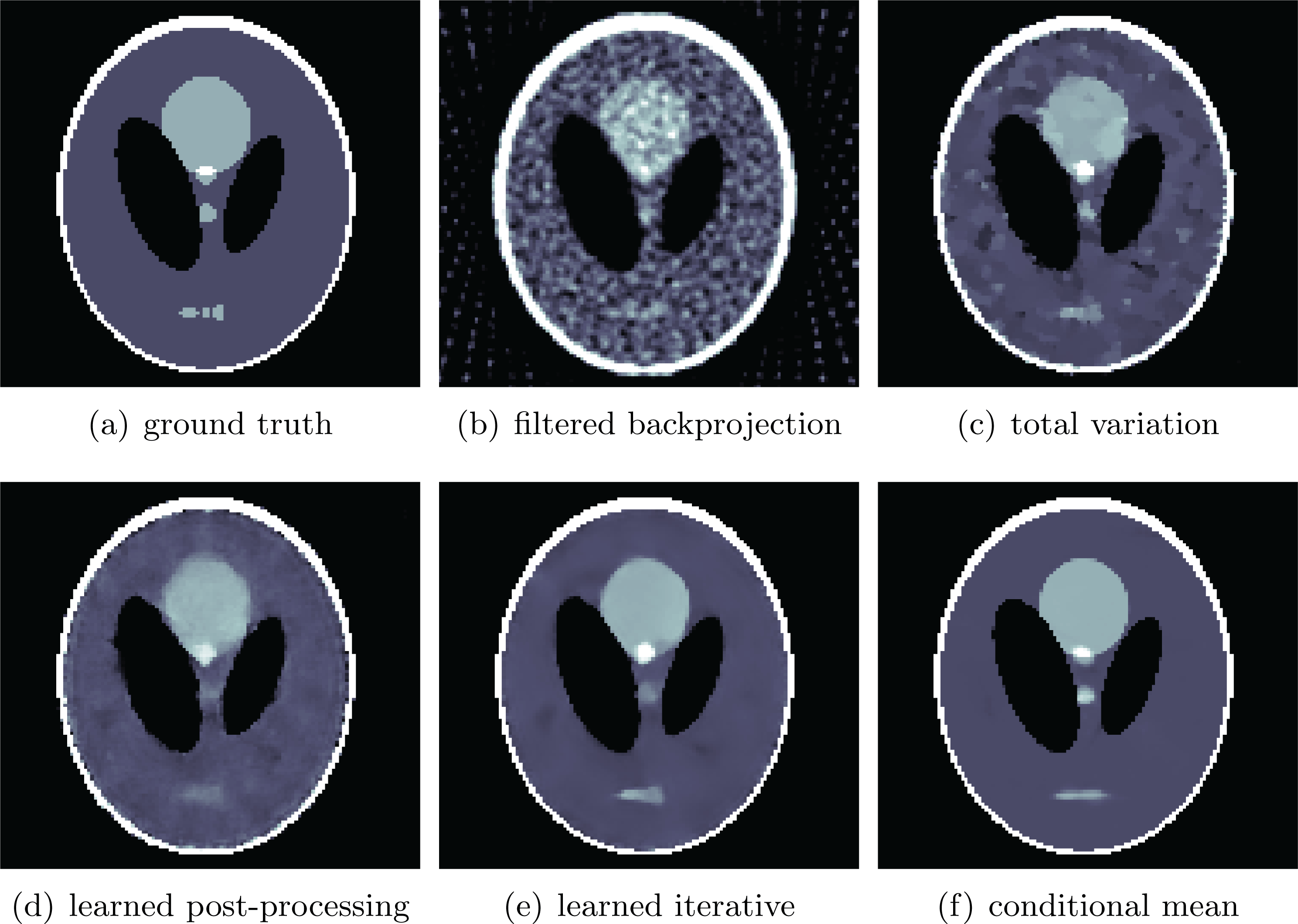
In the realistic setting shown in Figure 7.9 (see also the summary in Table 7.5) the images are clinical CT scans. We use supervised training data consisting of about 2000 pairs of images from nine patients, and corresponding pre-log data are simulated with a Poisson noise corresponding to
 $10^{4}$
incident photons per pixel before attenuation, which would correspond to a low-dose CT scan. Unfortunately we cannot compute the conditional mean as in the simplified setting, but we could compare against another approach for computing the conditional mean, namely a sampling-based approach based on a conditional GAN (see Section 5.2.1 and in particular Figure 7.16).
$10^{4}$
incident photons per pixel before attenuation, which would correspond to a low-dose CT scan. Unfortunately we cannot compute the conditional mean as in the simplified setting, but we could compare against another approach for computing the conditional mean, namely a sampling-based approach based on a conditional GAN (see Section 5.2.1 and in particular Figure 7.16).
Reconstructions of a
 $512\times 512$
pixel human phantom along with two zoom-in regions indicated by small circles. The left zoom-in has a true feature whereas texture in the right zoom-in is uniform. The window is set to
$512\times 512$
pixel human phantom along with two zoom-in regions indicated by small circles. The left zoom-in has a true feature whereas texture in the right zoom-in is uniform. The window is set to
 $[-200,200]$
Hounsfield units. Among the methods tested, only the learned iterative method (learned primal–dual algorithm) correctly recovers these regions. In the others, the true feature in the left zoom-in is indistinguishable from other false features of the same size/contrast, and the right-zoom in has a streak artefact. The improvement that comes with using a learned iterative method thus translates into true clinical usefulness.
$[-200,200]$
Hounsfield units. Among the methods tested, only the learned iterative method (learned primal–dual algorithm) correctly recovers these regions. In the others, the true feature in the left zoom-in is indistinguishable from other false features of the same size/contrast, and the right-zoom in has a streak artefact. The improvement that comes with using a learned iterative method thus translates into true clinical usefulness.
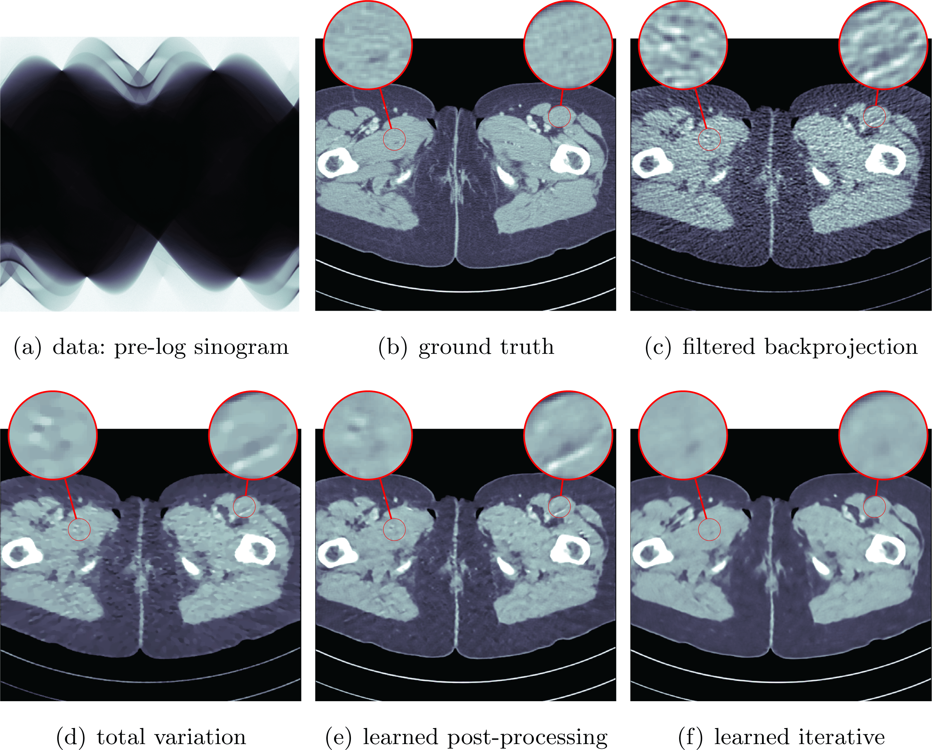
Summary of results shown in Figures 7.8 and 7.9 where an SSIM score of
 $1$
corresponds to a perfect match. Note that the learned iterative method (learned primal–dual algorithm) significantly outperforms TV regularization even when reconstructing the Shepp–Logan phantom. With respect to run-time, the learned iterative method involves calls to the forward operator, and is therefore slower than learned post-processing by a factor of
$1$
corresponds to a perfect match. Note that the learned iterative method (learned primal–dual algorithm) significantly outperforms TV regularization even when reconstructing the Shepp–Logan phantom. With respect to run-time, the learned iterative method involves calls to the forward operator, and is therefore slower than learned post-processing by a factor of
 ${\approx}6$
. Compared with TV-regularized reconstruction, all learned methods are at least two orders of magnitude faster.
${\approx}6$
. Compared with TV-regularized reconstruction, all learned methods are at least two orders of magnitude faster.
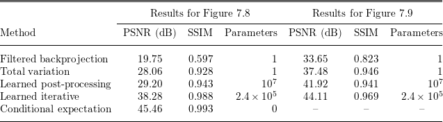
7.3.2 PAT reconstructions
Photoacoustic tomography (PAT) is a novel ‘imaging from coupled physics’ technique (Arridge and Scherzer Reference Arridge and Scherzer2012) that can obtain high-resolution three-dimensional in vivo images of absorbed optical energy by sensing laser-generated ultrasound (US) (Wang Reference Wang2009, Beard Reference Beard2011, Nie and Chen Reference Nie and Chen2014, Valluru, Wilson and Willmann Reference Valluru, Wilson and Willmann2016, Zhou, Yao and Wang Reference Zhou, Yao and Wang2016, Xia and Wang Reference Xia and Wang2014). In the setting considered here, data are collected as a time series on a two-dimensional sensor
 $Y=[\unicode[STIX]{x1D6E4}\subset \mathbb{R}^{2}]\times [0,T]$
on the surface of a domain
$Y=[\unicode[STIX]{x1D6E4}\subset \mathbb{R}^{2}]\times [0,T]$
on the surface of a domain
 $X=\unicode[STIX]{x1D6FA}\subset \mathbb{R}^{3}$
. Several methods exist for reconstruction, including filtered backprojection-type inversions of the spherical Radon transform and numerical techniques such as time-reversal. As in problems such as CT (Section 2.2.4) and MRI (Section 2.2.5), data subsampling may be employed to accelerate image acquisition, which leads consequently to the need for regularization to prevent noise propagation and artefact generation. The long reconstruction times ensuing from conventional iterative reconstruction algorithms have motivated consideration of machine learning methods.
$X=\unicode[STIX]{x1D6FA}\subset \mathbb{R}^{3}$
. Several methods exist for reconstruction, including filtered backprojection-type inversions of the spherical Radon transform and numerical techniques such as time-reversal. As in problems such as CT (Section 2.2.4) and MRI (Section 2.2.5), data subsampling may be employed to accelerate image acquisition, which leads consequently to the need for regularization to prevent noise propagation and artefact generation. The long reconstruction times ensuing from conventional iterative reconstruction algorithms have motivated consideration of machine learning methods.
The deep gradient descent (DGD) method (Hauptmann et al. Reference Hauptmann, Lucka, Betcke, Huynh, Adler, Cox, Beard, Ourselin and Arridge2018) for PAT is an example of a learned iterative method (see Section 5.1.4). The main aspects can be summarized as follows.
∙ Each iteration adds an update by combining measurement information delivered via the gradient
$\unicode[STIX]{x1D6FB}{\mathcal{L}}(g,{\mathcal{A}}f_{k})={\mathcal{A}}^{\ast }({\mathcal{A}}f_{k}-g)$
with an image processing step (7.7)where the layer operators$$\begin{eqnarray}f_{k+1}=\text{G}_{\unicode[STIX]{x1D703}_{k}}(\unicode[STIX]{x1D6FB}{\mathcal{L}}(g,{\mathcal{A}}f_{k}),f_{k}),\end{eqnarray}$$
$\text{G}_{\unicode[STIX]{x1D703}_{k}}$
correspond to partial differential equations (CNNs) with different, learned parameters
$\unicode[STIX]{x1D703}_{k}$
but with the same architecture. The initialization for the iterations was the backprojection of the data
$f_{0}={\mathcal{A}}^{\ast }g$
.∙ The training data were taken from the publicly available data from the ELCAP Public Lung Image Database.Footnote 9 The data set consists of 50 whole-lung CT scans, from which about 1200 volumes of vessel structures were segmented, and scaled up to the final target size of
$80\times 240\times 240$
. Out of these volumes 1024 were chosen as the ground truth
$f_{\text{true}}$
for the training and simulated limited-view, subsampled data, using the same measurement set-up as in the in vivo data. Precomputing the gradient information for each CNN took about 10 hours.∙ Initial results from training on synthetic data showed a failure to effectively threshold the noise-like artefacts in the low absorption regions (see Figure 7.10). This effect was ameliorated by simulating the effect of the low absorbing background as a Gaussian random field with short spatial correlation length. The synthetic CT volumes with the added background were then used for the data generation, i.e.
$g_{\text{back}}^{i}={\mathcal{A}}f_{\text{back}}^{i}+\unicode[STIX]{x1D700}$
, whereas the clean volumes
$f_{\text{true}}$
were used as reference for the training.∙ The results were further improved using transfer training with a set of 20 (fully sampled) measurements of a human finger, wrist and palm from the same experimental system. To update the DGD an additional five epochs of training on the pairs
$\{g_{\text{real}},f_{\operatorname{TV}}\}$
were performed with a reduced learning rate taking only 90 minutes. The effect of the updated deep gradient descent (DGD) is shown in Figure 7.11.


Reconstruction from real measurement data of a human palm, without adjustments of the training data. The images shown are top-down maximum intensity projections. (a) Result of the deep gradient descent (DGD) trained on images without added background. (b) TV reconstruction obtained from fully sampled data.
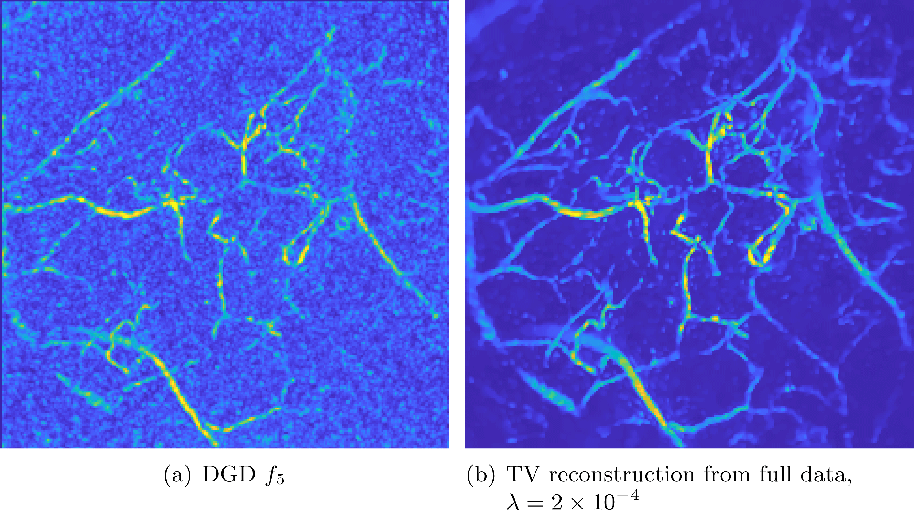
Example of real measurement data of a human palm. Volumetric images are shown using top-down maximum intensity projections. (a) Initialization from subsampled data, and (b) the DGD
 $G_{\hat{\unicode[STIX]{x1D703}}_{k}}$
after five iterations. (c) TV reconstruction of subsampled data with an emphasis on the data fit. (d) Reference TV reconstruction from fully sampled limited-view data. All TV reconstructions were computed with 20 iterations.
$G_{\hat{\unicode[STIX]{x1D703}}_{k}}$
after five iterations. (c) TV reconstruction of subsampled data with an emphasis on the data fit. (d) Reference TV reconstruction from fully sampled limited-view data. All TV reconstructions were computed with 20 iterations.
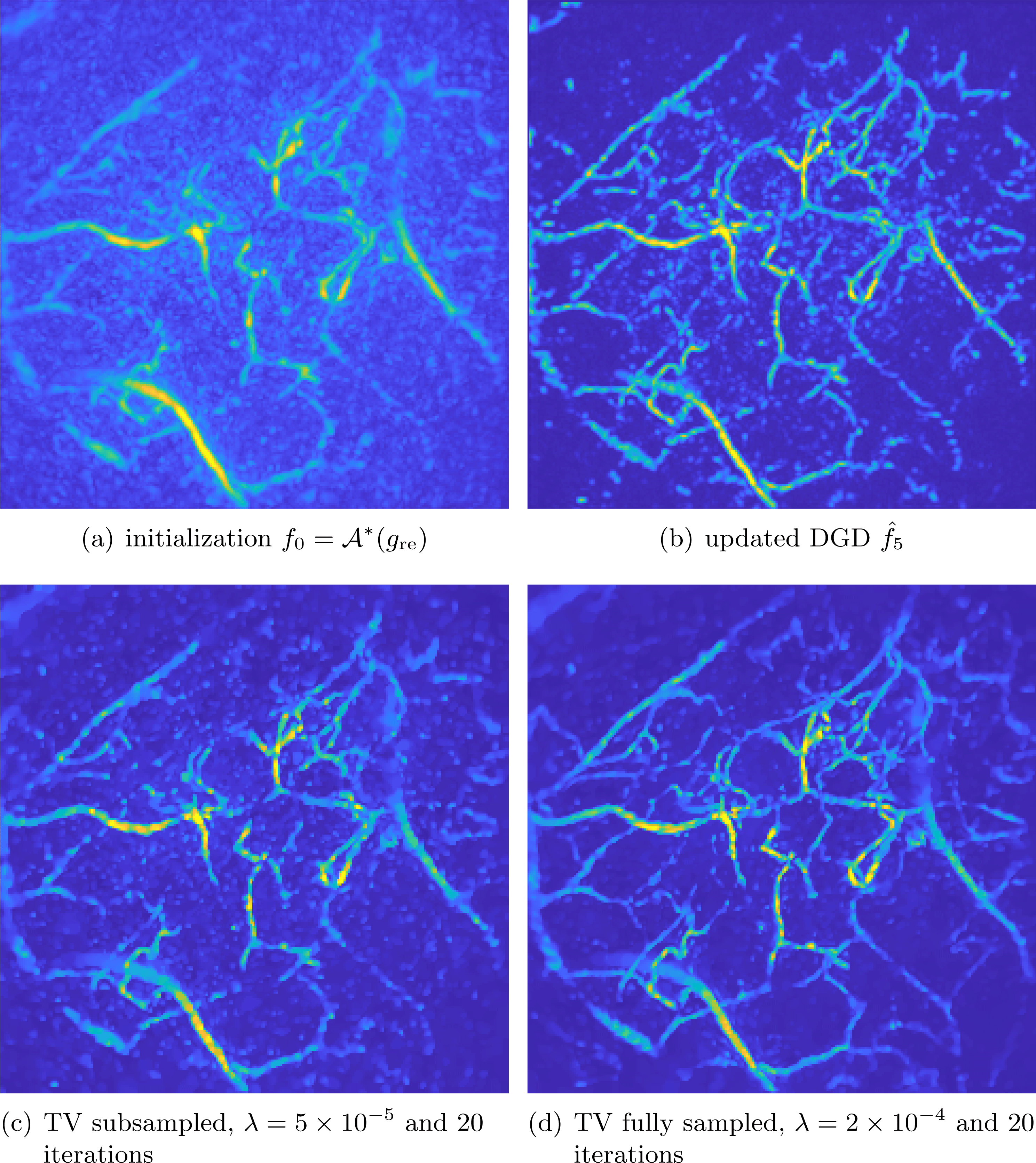
7.4 Adversarial regularizer for CT
In Section 4.7 the concept of training a regularizer that is parametrized with a neural network in an adversarial manner has been presented. In what follows, we present numerical results as they are reported in Lunz et al. (Reference Lunz, Öktem, Schönlieb and Bengio2018). There, the performance of the adversarial regularizer for two-dimensional CT reconstruction is considered, that is,
 ${\mathcal{A}}$
is the ray transform as in (2.6). CT reconstruction is an application in which functional analytic inversion (see Section 2), and in particular the variational approach from Sections 2.5 and 2.6, is very widely used in practice. Here, it serves as a prototype inverse problem with non-trivial forward operator.
${\mathcal{A}}$
is the ray transform as in (2.6). CT reconstruction is an application in which functional analytic inversion (see Section 2), and in particular the variational approach from Sections 2.5 and 2.6, is very widely used in practice. Here, it serves as a prototype inverse problem with non-trivial forward operator.
We compare the performance of TV-regularized reconstruction from Section 2.6 and (2.12), post-processing as in Section 5.1.5 (see in particular Gupta et al. Reference Gupta, Jin, Nguyen, McCann and Unser2018), RED in Section 4.6 and the adversarial regularizer from Section 4.7 on the LIDC/IDRI database (Armato et al. Reference Armato, McLennan, Bidaut, McNitt-Gray, Meyer, Reeves, Zhao, Aberle, Henschke and Hoffman2011) of lung scans.
We used a simple eight-layer convolutional neural network with a total of four average pooling layers of window size
 $2\times 2$
, leaky ReLU (
$2\times 2$
, leaky ReLU (
 $\unicode[STIX]{x1D6FC}=0.1$
) activations and two final dense layers for all experiments with the adversarial regularizer algorithm. Training and test measurements have been simulated by taking the ray transform of the two-dimensional CT slices, adding Gaussian white noise, and under-sampling the data by storing only
$\unicode[STIX]{x1D6FC}=0.1$
) activations and two final dense layers for all experiments with the adversarial regularizer algorithm. Training and test measurements have been simulated by taking the ray transform of the two-dimensional CT slices, adding Gaussian white noise, and under-sampling the data by storing only
 $30$
angles in the forward operator. Results are reported in Table 7.6 and Figure 7.12.
$30$
angles in the forward operator. Results are reported in Table 7.6 and Figure 7.12.
In Table 7.6 we see that TV is outperformed by the learned regularization techniques by a large margin. The reconstructions achieved by the adversarial regularizer are at least as good in visual quality as those obtained with supervised machine learning methods, despite having used unsupervised data only. The ability of the adversarial regularizer to be trained in an unsupervised fashion could be interesting for its application to practical inverse problems, where ground truth data are often scarce or unavailable. Further results of the adversarial regularizer and discussion can be found in Lunz et al. (Reference Lunz, Öktem, Schönlieb and Bengio2018).
CT reconstruction on the LIDC dataset using various methods. Note that the learned post-processing and RED methods require training on supervised data, while the adversarial regularizer only requires training on unsupervised data.
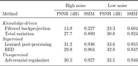
Exemplar CT reconstructions on the LIDC dataset under low-noise corruption. (a, b) Left to right: ground truth, FBP, TV, post-processing and adversarial regularization. (c,d) Data (CT sinograms): (c) data used for reconstructions in (a); (d) data used for reconstructions in (b).
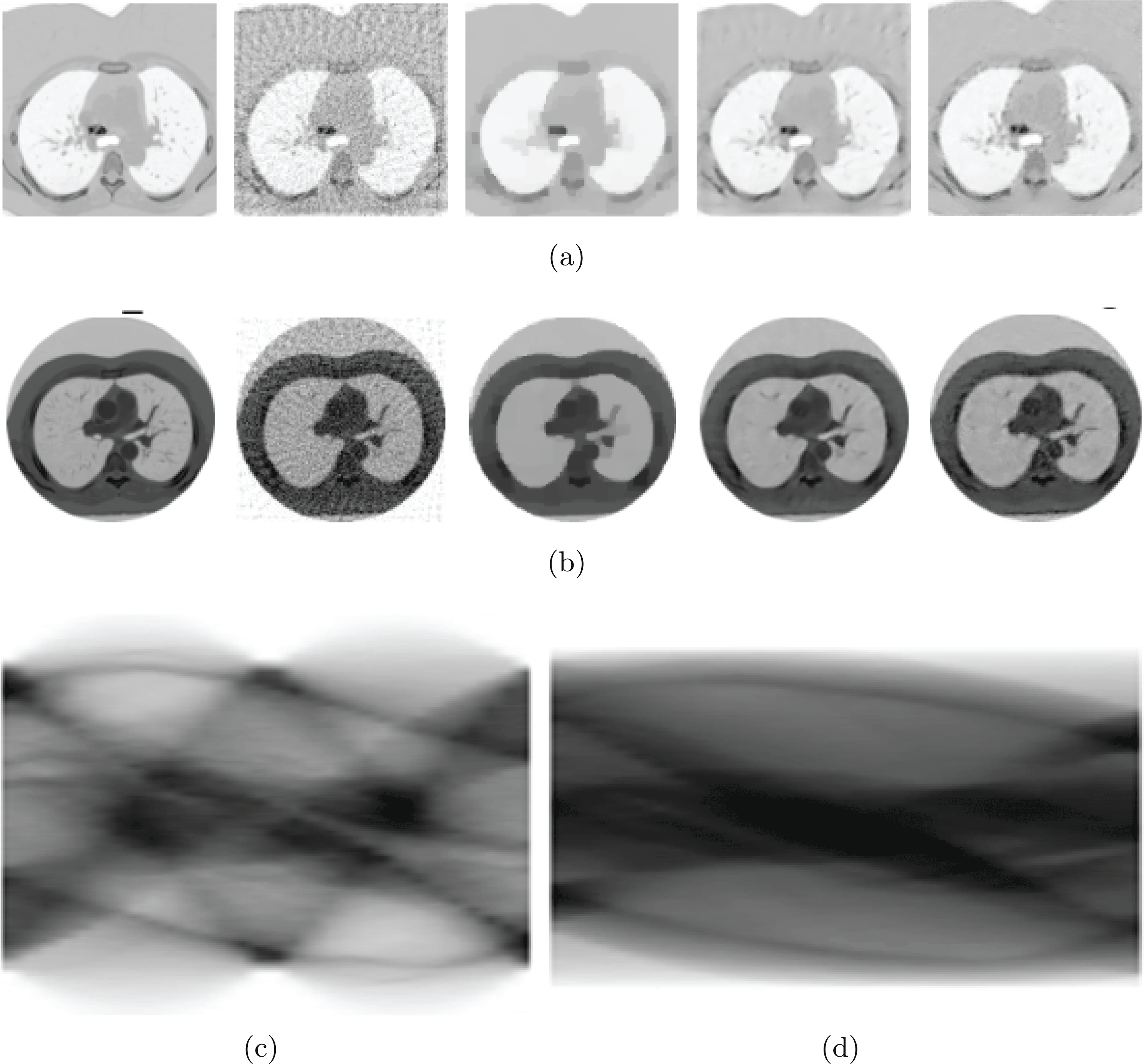
7.5 Deep learning for magnetic particle imaging (MPI)
MPI is an imaging modality based on injecting ferromagnetic nanoparticles, which are then transported by the blood flow. Reconstructing the resulting spatial distribution
 $c(x)$
of those nanoparticles is based on exploiting the non-linear magnetization behaviour of ferromagnetic nanoparticles (Gleich and Weizenecker Reference Gleich and Weizenecker2005).
$c(x)$
of those nanoparticles is based on exploiting the non-linear magnetization behaviour of ferromagnetic nanoparticles (Gleich and Weizenecker Reference Gleich and Weizenecker2005).
More precisely, one applies a magnetic field, which is a superposition of a static gradient field, which generates a field-free point (FFP), and a highly dynamic spatially homogeneous field, which moves the FFP in space. The magnetic moment of the nanoparticles in the neighbourhood of the field-free point will oscillate, generating an electromagnetic field whose voltages can be measured by so-called receive coils. The time-dependent measurements
 $v_{\ell }(t)$
in the receive coils are the data for the inversion process, i.e. for reconstructing
$v_{\ell }(t)$
in the receive coils are the data for the inversion process, i.e. for reconstructing
 $c(x)$
.
$c(x)$
.
MPI benefits from a high temporal resolution and a potentially high spatial resolution which makes it suitable for several in vivo applications, such as imaging blood flow (Weizenecker et al. Reference Weizenecker, Gleich, Rahmer, Dahnke and Borgert2009, Khandhar et al. Reference Khandhar, Keselman, Kemp, Ferguson, Goodwill, Conolly and Krishnan2017), instrument tracking (Haegele et al. Reference Haegele, Rahmer, Gleich, Borgert, Wojtczyk, Panagiotopoulos, Buzug, Barkhausen and Vogt2012) and guidance (Salamon et al. Reference Salamon, Hofmann, Jung, Kaul, Werner, Them, Reimer, Nielsen, vom Scheidt, Adam, Knopp and Ittrich2016), flow estimation (Franke et al. Reference Franke, Lacroix, Lehr, Heidenreich, Heinen and Schulz2017), cancer detection (Yu et al. Reference Yu, Bishop, Zheng, Ferguson, Khandhar, Kemp, Krishnan, Goodwill and Conolly2017) and treatment by hyperthermia (Murase et al. Reference Murase, Aoki, Banura, Nishimoto, Mimura, Kuboyabu and Yabata2015). However, real-time applications are still far from being realized; also, the mathematical foundation of such dynamic inverse problems (see Schmitt and Louis Reference Schmitt and Louis2002, Hahn Reference Hahn2015, Schuster, Hahn and Burger Reference Schuster, Hahn and Burger2018) is just developing.
Due to the non-magnetic coating of the nanoparticles, which largely suppresses particle–particle interactions, MPI is usually modelled by a linear Fredholm integral equation of the first kind describing the relationship between particle concentration and the measured voltage. After subtracting the voltage induced by the applied magnetic field one obtains a measured signal in the
 $\ell$
th receive coil as
$\ell$
th receive coil as
 $$\begin{eqnarray}y_{\ell }(t)=S_{\ell }c(t):=\int _{\unicode[STIX]{x1D6FA}}~c(x)~s_{\ell }(x,t)\text{d}t,\end{eqnarray}$$
where
 $s_{\ell }$
denotes the kernel of the linear operator. Combining the measurements of all receive coils yields – after discretization – a linear system of equations
$s_{\ell }$
denotes the kernel of the linear operator. Combining the measurements of all receive coils yields – after discretization – a linear system of equations
 $Sc=g$
. Typically, the rows of
$Sc=g$
. Typically, the rows of
 $S$
are normalized, resulting in the final form of the linearized inverse problem denoted by
$S$
are normalized, resulting in the final form of the linearized inverse problem denoted by
 $$\begin{eqnarray}\mathbf{\mathsf{A}}c=g.\end{eqnarray}$$
This is a coarse simplification of the physical set-up, which neglects non-linear magnetization effects of the nanoparticles as well as the non-homogeneity of the spatial sensitivity of the receive coils and also the small but non-negligible particle–particle interactions. Hence this is a perfect set-up for exploiting the potential of neural networks for matching complex and high-dimensional non-linear models.
We test the capability of the deep imaging prior approach to improving image reconstruction obtained by standard Tikhonov regularization. For the experiments we use datasets generated by the Bruker preclinical MPI system at the University Medical Center, Hamburg–Eppendorf.
We use the deep image prior network introduced by Ulyanov et al. (Reference Ulyanov, Vedaldi and Lempitsky2018), specifically their U-Net architecture. Our implementation is based on TensorFlow (Abadi et al.
Reference Abadi2015) and Keras (Chollet et al.
Reference Chollet2015), and has the following specifications. Between the encoder and decoder part of the U-Net our skip connection has four channels. The convolutional encoder goes from the input to 32, 32, 64 and 128 channels, each with strides of
 $2\times 2$
and filters of size
$2\times 2$
and filters of size
 $3\times 3$
. Then the convolutional decoder has the mirrored architecture plus first a resize-nearest-neighbour layer to reach the desired output shape and second an additional ReLU convolutional layer with filters of size
$3\times 3$
. Then the convolutional decoder has the mirrored architecture plus first a resize-nearest-neighbour layer to reach the desired output shape and second an additional ReLU convolutional layer with filters of size
 $1$
. The number of channels of this last layers is three for data set 1 (DS1) to accommodate three slices (three two-dimensional scans, one above another) of a two-dimensional phantom centred at the central slice of the three. The input of the network is given by a fixed Gaussian random input of size
$1$
. The number of channels of this last layers is three for data set 1 (DS1) to accommodate three slices (three two-dimensional scans, one above another) of a two-dimensional phantom centred at the central slice of the three. The input of the network is given by a fixed Gaussian random input of size
 $1\times 32\times 32$
.
$1\times 32\times 32$
.
For comparison with our deep inverse prior MPI reconstructions, we also compute sparse and classical Tikhonov reconstructions. We produce the Tikhonov reconstruction, usually associated with the minimization of the functional
 $$\begin{eqnarray}\Vert \!\mathbf{\mathsf{A}}c-g\Vert ^{2}+\unicode[STIX]{x1D706}\Vert c\Vert ^{2},\end{eqnarray}$$
via the algebraic reconstruction technique (Kaczmarz) as generalized to allow for the constraint
 $x\geq 0$
by Dax (Reference Dax1993). We produce the sparsity reconstruction, usually associated with the minimization of the functional
$x\geq 0$
by Dax (Reference Dax1993). We produce the sparsity reconstruction, usually associated with the minimization of the functional
 $$\begin{eqnarray}\Vert \!\mathbf{\mathsf{A}}c-g\Vert ^{2}+\unicode[STIX]{x1D706}\Vert c\Vert _{1},\end{eqnarray}$$
by simply implementing this functional in TensorFlow and minimizing it via gradient descent. In the end we set all negative entries to
 $0$
.
$0$
.
MPI reconstructions of two phantoms using different methods: (a)–(d) phantom with 4 mm distance between tubes containing ferromagnetic nanoparticles; (e)–(h) phantom with 2 mm distance. The methods used are Kaczmarz with
 $L^{2}$
-discrepancy (
$L^{2}$
-discrepancy (
 $\tilde{\unicode[STIX]{x1D706}}=5\times 10^{-4}$
),
$\tilde{\unicode[STIX]{x1D706}}=5\times 10^{-4}$
),
 $\ell _{1}$
-regularization (
$\ell _{1}$
-regularization (
 $\tilde{\unicode[STIX]{x1D706}}=5\times 10^{-3}$
) and DIP (
$\tilde{\unicode[STIX]{x1D706}}=5\times 10^{-3}$
) and DIP (
 $\unicode[STIX]{x1D702}=5\times 10^{-5}$
) for both cases. Photos of phantoms taken by T. Kluth at the University Medical Center, Hamburg–Eppendorf.
$\unicode[STIX]{x1D702}=5\times 10^{-5}$
) for both cases. Photos of phantoms taken by T. Kluth at the University Medical Center, Hamburg–Eppendorf.
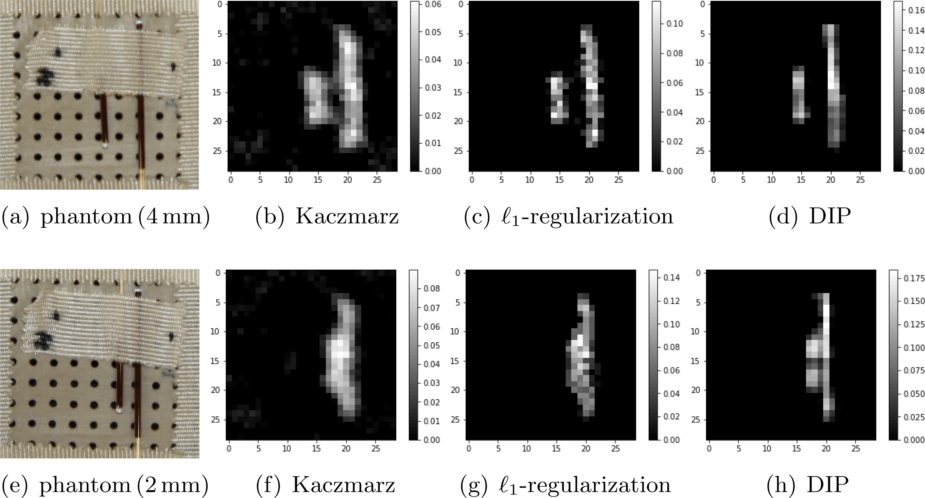
We start by presenting direct comparisons of the Kaczmarz, sparsity and DIP reconstructions in Figure 7.13. Beneath each image we state the parameters we used for the reconstruction
 $\tilde{\unicode[STIX]{x1D706}}=\Vert \!\mathbf{\mathsf{A}}\Vert _{F}^{2}\unicode[STIX]{x1D706}$
, where
$\tilde{\unicode[STIX]{x1D706}}=\Vert \!\mathbf{\mathsf{A}}\Vert _{F}^{2}\unicode[STIX]{x1D706}$
, where
 $\Vert \cdot \Vert _{F}$
denotes the Frobenius norm and
$\Vert \cdot \Vert _{F}$
denotes the Frobenius norm and
 $\unicode[STIX]{x1D706}$
is the regularization parameter as used in (7.9) or (7.10) and
$\unicode[STIX]{x1D706}$
is the regularization parameter as used in (7.9) or (7.10) and
 $\unicode[STIX]{x1D702}$
the learning rate used in training the network. For DIP we always used early stopping after
$\unicode[STIX]{x1D702}$
the learning rate used in training the network. For DIP we always used early stopping after
 $1000$
optimization steps. The images started to deteriorate slowly for more iterations. For implementation details, as well as further numerical examples also showing the limitation of the DIP approach, see Dittmer et al. (Reference Dittmer, Kluth, Maass and Baguer2018).
$1000$
optimization steps. The images started to deteriorate slowly for more iterations. For implementation details, as well as further numerical examples also showing the limitation of the DIP approach, see Dittmer et al. (Reference Dittmer, Kluth, Maass and Baguer2018).
7.6 Task-based reconstruction
We demonstrate the framework of Section 6.1 on joint tomographic image reconstruction and segmentation of white brain matter.
 ${\mathcal{R}}_{\unicode[STIX]{x1D703}}$
is given by a learned primal–dual method (Adler and Öktem Reference Adler and Öktem2018b
), which incorporates a knowledge-based model for how data are generated into its architecture, and
${\mathcal{R}}_{\unicode[STIX]{x1D703}}$
is given by a learned primal–dual method (Adler and Öktem Reference Adler and Öktem2018b
), which incorporates a knowledge-based model for how data are generated into its architecture, and
 ${\mathcal{T}}_{\unicode[STIX]{x1D719}}$
is given by a U-Net (Ronneberger, Fischer and Brox Reference Ronneberger, Fischer, Brox and Navab2015).
${\mathcal{T}}_{\unicode[STIX]{x1D719}}$
is given by a U-Net (Ronneberger, Fischer and Brox Reference Ronneberger, Fischer, Brox and Navab2015).
Some results are shown in Figure 7.14. Note in particular that (perhaps surprisingly) the ‘best’ segmentation is not obtained by a fully end-to-end approach: instead they are obtained when the reconstruction loss is included as a regularizer. Furthermore, it is clear that the reconstruction obtained for
 $C=0.9$
over-emphasizes image features relevant for the task, for example white–grey matter contrast. This clearly ‘helps’ the task and also visually shows the image features used by the joint approach.
$C=0.9$
over-emphasizes image features relevant for the task, for example white–grey matter contrast. This clearly ‘helps’ the task and also visually shows the image features used by the joint approach.
Joint tomographic reconstruction and segmentation of grey matter. Images shown using a
 $[-100,100]$
HU window and segmentation using a
$[-100,100]$
HU window and segmentation using a
 $[0,1]$
window. The choice
$[0,1]$
window. The choice
 $C=0.9$
seems to be a good compromise for good reconstruction and segmentation, so clearly it helps to use a loss that includes the reconstruction and not only the task.
$C=0.9$
seems to be a good compromise for good reconstruction and segmentation, so clearly it helps to use a loss that includes the reconstruction and not only the task.
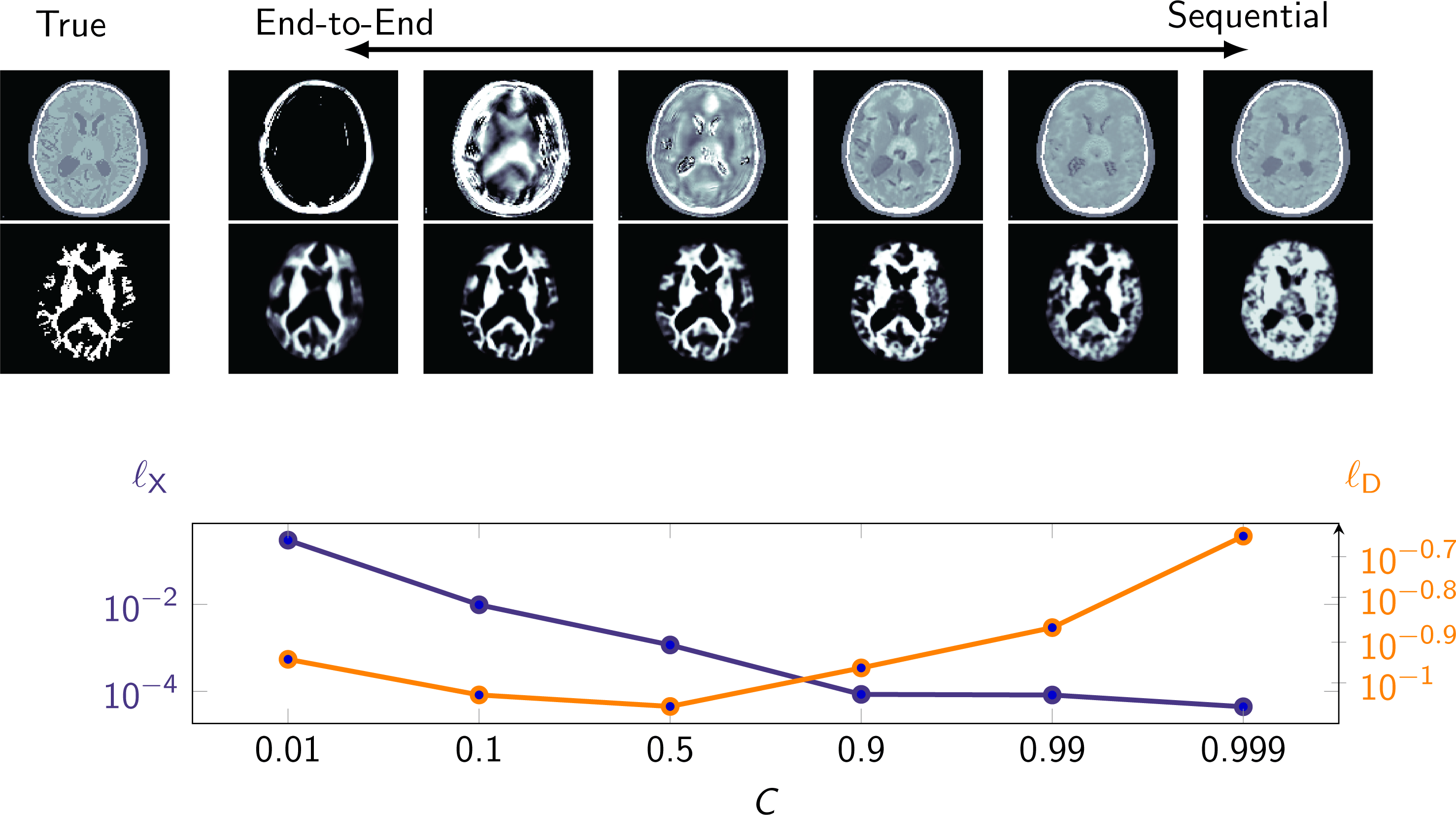
7.7 Clinical image guided decision making
We show how to compute an estimator relevant for uncertainty quantification in the context of CT image reconstruction. As a practical example, we will compute a CT reconstruction from ultra-low-dose data (Figure 7.15(a)). The aim is to identify a feature (a potential tumour) and then seek to estimate the likelihood of its presence.
Formalizing the above, let
 $\unicode[STIX]{x1D6E5}$
denote the difference in mean intensity in the reconstructed image between a region encircling the feature and the surrounding organ, which in our example is the liver. The feature is said to ‘exist’ whenever
$\unicode[STIX]{x1D6E5}$
denote the difference in mean intensity in the reconstructed image between a region encircling the feature and the surrounding organ, which in our example is the liver. The feature is said to ‘exist’ whenever
 $\unicode[STIX]{x1D6E5}$
is bigger than a certain threshold, say
$\unicode[STIX]{x1D6E5}$
is bigger than a certain threshold, say
 $10$
Hounsfield units.
$10$
Hounsfield units.
Test data: (a) subset of CT data from an ultra-low-dose three-dimensional helical scan and (b) the corresponding FBP reconstruction. Images are shown using a display window set to
 $[-150,200]$
Hounsfield units.
$[-150,200]$
Hounsfield units.
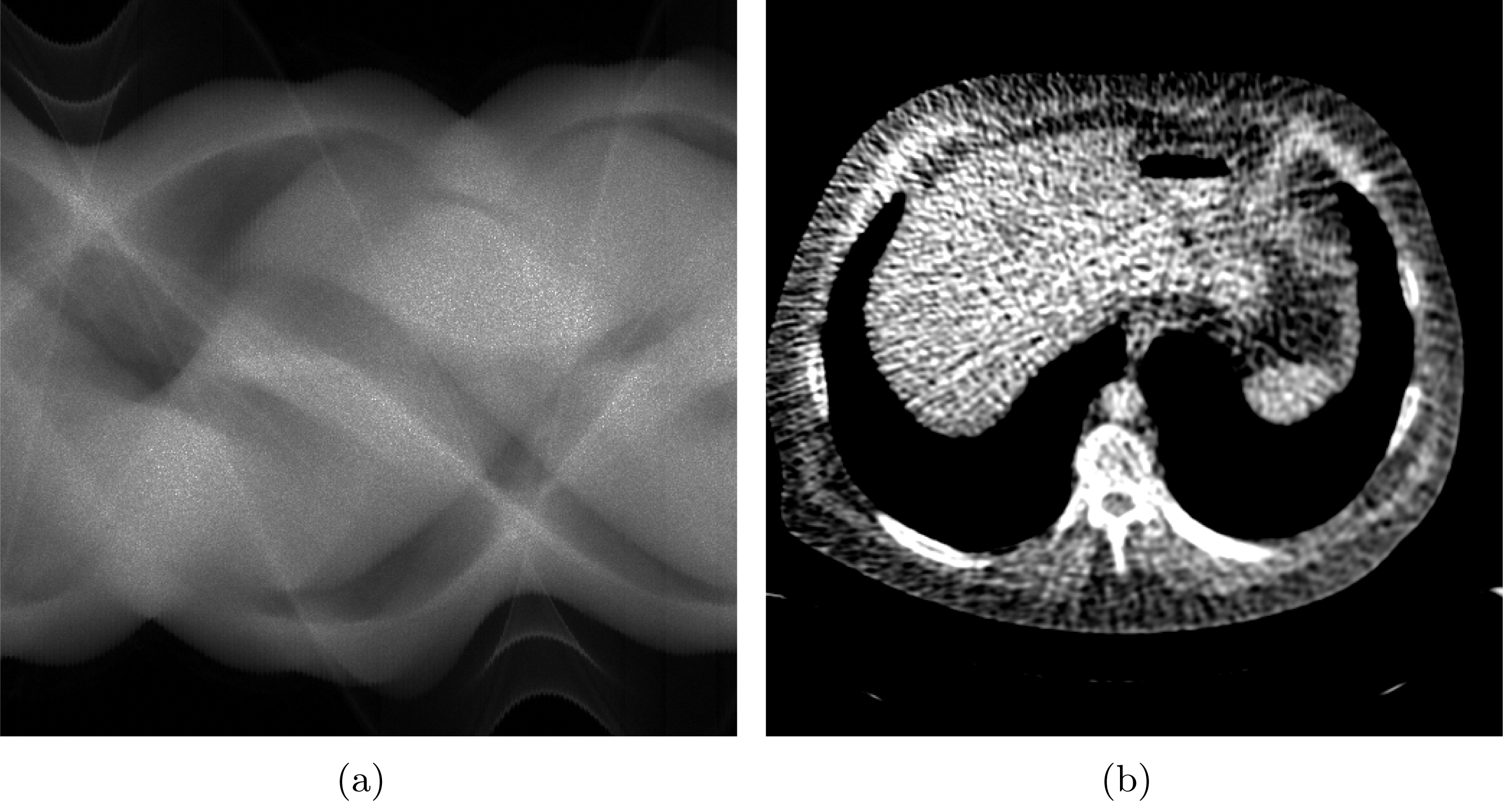
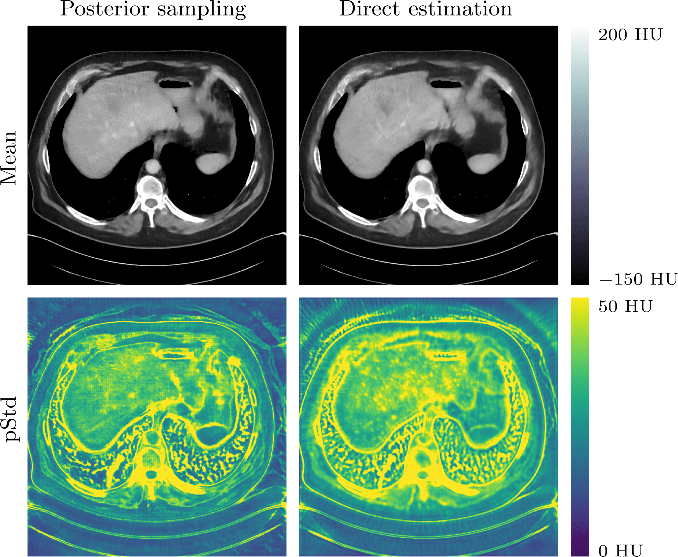
(b) Suspected tumour (red) and reference region (blue) shown in the sample posterior mean image. (c) Average contrast differences between the tumour and reference region. The histogram is computed by posterior sampling applied to test data (Figure 7.15); the yellow curve is from direct estimation (Section 5.1.6), and the true value is the red threshold. (a) The normal dose image that confirms the presence of the feature.
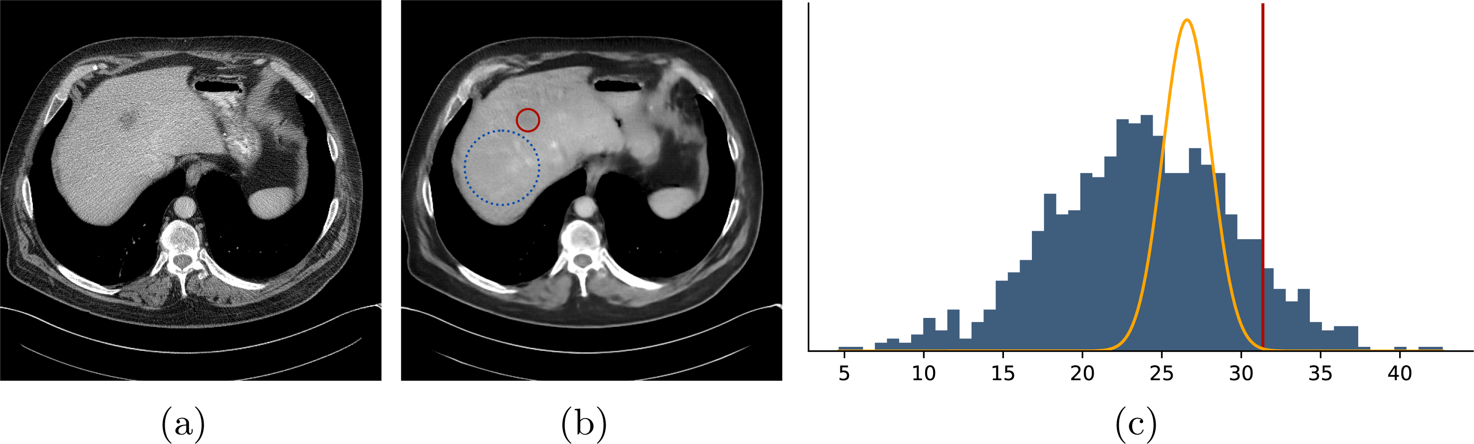
To use posterior sampling, start by computing the conditional mean image (top left in Figure 7.16) by sampling from the posterior using the conditional Wasserstein GAN approach in Section 5.2.1. There is a ‘dark spot’ in the liver (a possible tumour) and a natural clinical question is to statistically test for the presence of this feature. To do this, compute
 $\unicode[STIX]{x1D6E5}$
for a number of samples generated by posterior sampling, which is the same 1000 samples used to compute the conditional mean. We estimate the probability
$\unicode[STIX]{x1D6E5}$
for a number of samples generated by posterior sampling, which is the same 1000 samples used to compute the conditional mean. We estimate the probability
 $p$
that
$p$
that
 $\unicode[STIX]{x1D6E5}>10$
Hounsfield units from the resulting histogram in Figure 7.17 and clearly
$\unicode[STIX]{x1D6E5}>10$
Hounsfield units from the resulting histogram in Figure 7.17 and clearly
 $p>0.95$
, indicating that the ‘dark spot’ feature exists with at least 95% significance. This is confirmed by the ground truth image (Figure 7.17(a)). The conditional mean image also under-estimates
$p>0.95$
, indicating that the ‘dark spot’ feature exists with at least 95% significance. This is confirmed by the ground truth image (Figure 7.17(a)). The conditional mean image also under-estimates
 $\unicode[STIX]{x1D6E5}$
, whose true value is the vertical line in Figure 7.17(c). This is to be expected since the prior introduces a bias towards homogeneous regions, a bias that decreases as the noise level decreases.
$\unicode[STIX]{x1D6E5}$
, whose true value is the vertical line in Figure 7.17(c). This is to be expected since the prior introduces a bias towards homogeneous regions, a bias that decreases as the noise level decreases.
To perform the above analysis using direct estimation, start by computing the conditional mean image from the same ultra-low-dose data using direct estimation. As expected, the resulting image (top right in Figure 7.16) shows a ‘dark spot’ in the liver. Now, designing and training a neural network that directly estimates the distribution of
 $\unicode[STIX]{x1D6E5}$
is unfeasible in a general setting. However, as shown in Section 5.1.6, this is possible if one assumes pixels are independent of each other. The estimated distribution of
$\unicode[STIX]{x1D6E5}$
is unfeasible in a general setting. However, as shown in Section 5.1.6, this is possible if one assumes pixels are independent of each other. The estimated distribution of
 $\unicode[STIX]{x1D6E5}$
is the curve in Figure 7.17 and we get
$\unicode[STIX]{x1D6E5}$
is the curve in Figure 7.17 and we get
 $p>0.95$
, which is consistent with the result obtained using posterior sampling. The direct estimation approach is based on assuming independent pixels, so it will significantly underestimate the variance. In contrast, the approach based on posterior sampling seems to give a more realistic estimate of the variance.
$p>0.95$
, which is consistent with the result obtained using posterior sampling. The direct estimation approach is based on assuming independent pixels, so it will significantly underestimate the variance. In contrast, the approach based on posterior sampling seems to give a more realistic estimate of the variance.
8 Conclusions and outlook
8.1 Summary
In this survey we have tried to capture the state of the art in the still relatively young and fast-emerging field of machine learning approaches for solving inverse problems.
Our journey has taken us from more familiar applications of data-driven methods, such as dictionary learning (Section 4.4), bilevel learning (Section 4.3) and learning Markov random field-type regularizers (Section 4.3.2) to recent advances in using deep neural networks to solve inverse problems (Sections 4.6–4.10 and 5.1). These approaches are surveyed together with a brief account of the underlying mathematical setting (Sections 1–3), and their performance in some key applications is shown in Section 7. Taken together, we hope this will convince the reader that inverse problems can profit from data-driven methods. This claim is further strengthened by showing how data-driven methods can be used to compensate for inaccuracies in the forward model (Section 6.2) and how one can adapt the reconstruction to a specific task (Section 6.1).
The examples in Section 7 clearly show that some of these methods are very promising, regarding both output quality and computational feasibility. Strong empirical evidence suggests that using problem-specific deep neural networks that include knowledge-driven models outperform purely knowledge- or data-driven approaches. In contrast, there is little rigorous mathematical theory supporting these empirical observations, but the results clearly show that it is worth the effort to develop the necessary theory.
Below are some further key observations we believe are worth pointing out regarding the role of deep learning in solving inverse problems.
The functional analytic and Bayesian viewpoints.
The way deep learning is used for solving an inverse problem depends on whether one adopts the functional analytic or the Bayesian viewpoint.
Within the functional analytic viewpoint, a deep neural network is simply a parametrized family of operators, and learning amounts to calibrating the parameters against example data by minimizing some appropriate loss function.
In Bayesian inversion, a deep neural network corresponds to a statistical decision rule, so methods from deep learning constitute a computational framework for statistical decision making in high dimensions. For example, many of the estimators that have previously been computationally unfeasible are now computable: for example, the conditional mean seems to be well approximated by learned iterative schemes (Section 5.1.4). Likewise, a trained generative network can be used to sample from the posterior (Section 5.2) in a computationally feasible manner, as shown in Section 5.2.
Computational feasibility.
Essentially all methods from Bayesian inversion and many from functional analytic regularization are computationally very demanding. Those techniques based on unrolling an iterative scheme (Section 4.9.1) are for designing a deep neural network that approximates a computationally demanding operator, such as one that solves a large-scale optimization problem.
The training of such a deep neural network may take quite some time, but once it is trained, it is fast to evaluate. In some sense, this is a way to redistribute the computational burden from the execution to the training.
Handling lack of training data.
Inverse problems in the sciences and engineering often have little training data compared to the dimensionality of the model parameter. Furthermore, it is impractical to have a method that requires retraining as soon as the measurement protocol changes. This becomes an issue is medical imaging where data in multi-centre studies is typically acquired using different CT or MRI scanners.
For these reasons, black-box machine learning algorithms (Section 7.1) are not suitable for solving such inverse problems. On the other hand, in these inverse problems there is often a knowledge-driven model for how data are generated and it is important to integrate this information into the data-driven method. Learned iterative schemes (Section 5.1.4) employ a deep neural network that embeds this model for data into its architecture.
Encoding a priori information.
In functional analytic regularization, much of the theoretical research (Section 2) has focused on finding optimal convergence rates as the noise level tends to zero. Likewise, theoretical research in Bayesian inversion (Section 3) focuses on contraction rates for certain classes of priors and in deriving an asymptotic closed-form characterization of the posterior distribution as the noise level tends to zero. Here, the regularization functional (in functional analytic regularization) and the prior distribution (in Bayesian inversion) primarily act as a regularizers.
The above viewpoint does not acknowledge the potential that lies in encoding knowledge about the true model parameter into the regularization functional or prior. Furthermore, in applications data are fixed with some given noise level, and there is little, if any, guidance from the above theory on which regularizer or prior to select in such a setting. Empirical evidence suggests that instead of hand-crafting a regularization functional or a prior, one can learn it from example data. This allows us to pick up information related to the inverse problem that is difficult, if not impossible, to account for otherwise.
Unrolling.
A key technique in many approaches for using deep learning to solve inverse problems is to construct problem-specific deep neural network architectures by unrolling an iterative scheme, as outlined in Section 4.9.1.
This technique allows us to use compressed sensing theory to derive properties for certain classes of deep neural networks, for example those resulting from ML-CSC (Section 4.4.2). Next, as shown in Section 4.9, the same technique is also useful in accelerating the evaluation of computationally demanding operators, such as those that solve large-scale optimization problems. Finally, unrolling is also used to embed a knowledge-driven forward operator and the adjoint of its derivative into a deep neural network that seeks to approximate an estimator (Section 5.1).
The above principle of unrolling can be used in a much wider context than solving an optimization problem or an inverse problem. It can be seen as constructing a deep neural network architecture for approximating an operator that is given implicitly through an iterative scheme. Hence, as pointed out in Section 4.9.4, unrolling establishes a link between numerical analysis and deep learning.
8.2 Outlook
We identify several interesting directions for future research in the context of inverse problems and machine learning.
8.2.1 Approximation and convergence properties of deep inversion
We believe a key component of future research is to analyse the mathematical–statistical approximation and convergence properties of inversion strategies that use deep neural networks, for example statistical recovery guarantees and generalization limits, as well as bounds on the number of training samples necessary for reaching prescribed accuracies, and estimates for uncertainty in terms of stability properties and statistical confidence statements for the algorithms used.
Convergence and stability properties of denoising by deep neural networks can be analysed using techniques from sparse signal processing, as in Papyan et al. (Reference Papyan, Romano and Elad2017). Likewise, techniques from applied harmonic analysis can be used to analyse approximation properties of feed-forward deep neural networks, as in Bölcskei et al. (Reference Bölcskei, Grohs, Kutyniok and Petersen2019). This paper establishes a connection between the complexity of a function class in
 $L^{2}(\mathbb{R}^{d})$
and the complexity (model capacity) of feed-forward deep neural networks approximating functions from this class to within a prescribed accuracy. A specific focus is on function classes in
$L^{2}(\mathbb{R}^{d})$
and the complexity (model capacity) of feed-forward deep neural networks approximating functions from this class to within a prescribed accuracy. A specific focus is on function classes in
 $L^{2}(\mathbb{R}^{d})$
that are optimally approximated by general affine systems, which include a wide range of representation systems from applied harmonic analysis such as wavelets, ridgelets, curvelets, shearlets,
$L^{2}(\mathbb{R}^{d})$
that are optimally approximated by general affine systems, which include a wide range of representation systems from applied harmonic analysis such as wavelets, ridgelets, curvelets, shearlets,
 $\unicode[STIX]{x1D6FC}$
-shearlets and, more generally,
$\unicode[STIX]{x1D6FC}$
-shearlets and, more generally,
 $\unicode[STIX]{x1D6FC}$
-molecules. The central result in Bölcskei et al. (Reference Bölcskei, Grohs, Kutyniok and Petersen2019) is that feed-forward deep neural networks achieve the optimum approximation properties of all affine systems combined with minimal connectivity and memory requirements.
$\unicode[STIX]{x1D6FC}$
-molecules. The central result in Bölcskei et al. (Reference Bölcskei, Grohs, Kutyniok and Petersen2019) is that feed-forward deep neural networks achieve the optimum approximation properties of all affine systems combined with minimal connectivity and memory requirements.
None of these papers, however, consider deep neural networks in the context of inverse problems.
8.2.2 Robustness against adversarial attacks
Sensitivity towards adversarial attacks is a known issue that has mostly been studied in the context of classification (Szegedy et al. Reference Szegedy, Zaremb, Sutskever, Bruna, Erhan, Goodfellow and Fergus2014); see also the surveys by Chakraborty et al. (Reference Chakraborty, Alam, Dey, Chattopadhyay and Mukhopadhyay2018) and Akhtar and Mian (Reference Akhtar and Mian2018). However, little work has been done regarding adversarial stability of reconstruction methods for solving inverse problems that are based on deep neural networks.
One recent work along these lines is that of Antun et al. (Reference Antun, Renna, Poon, Adcock and Hansen2019), who extend the approach in Szegedy et al. (Reference Szegedy, Zaremb, Sutskever, Bruna, Erhan, Goodfellow and Fergus2014) to the case of regression. The idea is to perturb the model parameter in a way that is hard to distinguish, yet the data from the perturbed model parameter have a large influence on the reconstruction. The perturbation (adversarial example) is computed by solving an optimization and, in contrast to classification, different optimization problems can be constructed to test for different types of instabilities. The adversarial stability test in Antun et al. (Reference Antun, Renna, Poon, Adcock and Hansen2019) is demonstrated on MRI image reconstruction. The paper tests two fully learned approaches given by Zhu et al. (Reference Zhu, Liu, Cauley, Rosen and Rosen2018) and Schlemper et al. (Reference Schlemper, Caballero, Hajnal, Price and Rueckert2018), two learned post-processing approaches given by Jin et al. (Reference Jin, McCann, Froustey and Unser2017) and Yang et al. (Reference Yang, Yu, Dong, Slabaugh, Dragotti, Ye, Liu, Arridge, Keegan, Guo and Firmin2018b ), and finally the learned iterative approach of Hammernik et al. (Reference Hammernik, Klatzer, Kobler, Recht, Sodickson, Pock and Knoll2018). All approaches show adversarial instability, which could come as a surprise for the learned iterative approach that seeks to approximate a conditional mean that is known to be stable (Section 3.2.2). One reason for this could be that the learned iterative approach of Hammernik et al. (Reference Hammernik, Klatzer, Kobler, Recht, Sodickson, Pock and Knoll2018), which is based on variational networks, has a model capacity too limited to properly approximate the conditional mean.
On a final note, a key element in Antun et al. (Reference Antun, Renna, Poon, Adcock and Hansen2019) is that data from the perturbation model parameter is noise-free. It is known that adding white noise to the input helps against adversarial attacks for classifiers (Cohen, Rosenfeld and Kolter Reference Cohen, Rosenfeld and Kolter2019). Moreover, in inverse problems one always has noisy data, so it remains unclear whether the computed perturbation in Antun et al. (Reference Antun, Renna, Poon, Adcock and Hansen2019) actually acts as an adversarial example when noise is added.
Clearly, theory for robustness against adversarial attacks in the context of inverse problems is very much an emerging field.
8.2.3 Theory for learned iterative reconstruction
More specifically, the theory of statistical regularization applied to learned iterative methods in Section 5.1.4 is fairly incomplete, especially when interested in theoretical guarantees in the presence of empirical distributions for the data and model parameter. This will require studying estimates of the posterior in a non-asymptotic setting. Another key element is to estimate the generalization gap for learned iterative methods. Here one could consider theory for empirical Bayes methods, but current results focus on analysing Bayesian inversion methods where hyper-parameters defining a hierarchical prior are selected from data (Knapik, Szabó, van der Vaart and van Zanten Reference Knapik, Szabó, van der Vaart and van Zanten2016, Szabó, van der Vaart and van Zanten Reference Szabó, van der Vaart and van Zanten2013).
8.2.4 ‘Convergence’ of training data
For all approaches where supervised training data are used, there is a discrepancy between theoretical error estimates in the infinite-dimensional setting and the practical case of finite-dimensional training data used in presented data-driven inversion approaches. For instance, error estimates are needed between solutions of a neural network trained on finitely many samples (that describe a particular empirical distribution) and solutions trained with infinitely many samples from a joint distribution.
8.2.5 Bespoke neural network architectures for inverse problems
In many inverse problems the model parameter space
 $X$
and the data space
$X$
and the data space
 $Y$
are not the same, and in particular the data
$Y$
are not the same, and in particular the data
 $g$
often live in non-Euclidean spaces. On the other hand, existing data-driven inversion models, as discussed in this survey, which make use of neural networks as data-driven parametrizations, usually employ off-the-shelf network architectures such as U-Net, for instance. For future research it would be interesting to investigate neural network architectures that are specifically designed as mappings between non-Euclidean spaces. Some developments along these lines can be found in the paper by Bronstein et al. (Reference Bronstein, Bruna, LeCun, Szlam and Vandergheynst2017), who investigate how the notion of a CNN can be generalized to non-Euclidean structures such as graphs and manifolds.
$g$
often live in non-Euclidean spaces. On the other hand, existing data-driven inversion models, as discussed in this survey, which make use of neural networks as data-driven parametrizations, usually employ off-the-shelf network architectures such as U-Net, for instance. For future research it would be interesting to investigate neural network architectures that are specifically designed as mappings between non-Euclidean spaces. Some developments along these lines can be found in the paper by Bronstein et al. (Reference Bronstein, Bruna, LeCun, Szlam and Vandergheynst2017), who investigate how the notion of a CNN can be generalized to non-Euclidean structures such as graphs and manifolds.
The above is also closely related to work in developing neural network architectures that are equivariant and/or invariant to certain transformations given as group action. This is highly relevant when one seeks to solve inverse problems whose solutions enjoy such equivariance and/or invariance. Examples of work in this direction are those of Esteves, Allen-Blanchette, Makadia and Daniilidis (Reference Esteves, Allen-Blanchette, Makadia and Daniilidis2017), Zhao et al. (Reference Zhao, Hu, Dotzel, Sa and Zhang2018), Weiler et al. (Reference Weiler, Geiger, Welling, Boomsma and Cohen2018) and Veeling et al. (Reference Veeling, Linmans, Winkens, Cohen and Welling2018), but none of this is pursued in the context of inverse problems.
Another feature of inverse problems is that one can often prescribe how singularities in data are related to those in the model parameter (Section 6.3). Hence it is natural to seek network architectures that encode not only the forward operator but also such a relation. This is likely to further improve the robustness and generalization properties.
8.2.6 Continuous notion of neural network architectures
Some of the recent attempts to build a continuous framework for neural networks have been touched upon in Section 6.2.1. Continuous formulations to neural networks make them amenable to the rich toolkit of functional analysis and theoretical results as outlined in Section 2. Moreover, starting with a continuous model such as a partial differential equation, for instance, may give rise to new discretizations and new neural network architectures – a development that has clearly happened before in mathematical imaging (e.g. Perona and Malik Reference Perona and Malik1990).
8.2.7 Theoretical guarantees for learning-to-optimize approaches
If a neural network is used to approximate and consequently computationally speed up a knowledge-driven approach (e.g. the learning-to-optimize methods in Section 4.9), it is important to understand the error committed by such an approximation. What is the correct notion of such an approximation error? How does it depend on the training set and the network architecture?
Acknowledgements
This article builds on lengthy discussions and long-standing collaborations with a large number of people. These include Jonas Adler, Sebastian Banert, Martin Benning, Marta Betcke, Luca Calatroni, Juan Carlos De Los Reyes, Andreas Hauptmann, Lior Horesh, Bangti Jin, Iasonas Kokkinos, Felix Lucka, Sebastian Lunz, Thomas Pock, Tuomo Valkonen and Olivier Verdier. The authors are moreover grateful to the following people for proofreading the manuscript and providing valuable feedback on its content and structure: Andrea Aspri, Martin Benning, Matthias Ehrhardt, Barbara Kaltenbacher, Yury Korolev, Mike McCann, Erkki Somersalo and Michael Unser.
SA acknowledges support from EPSRC grant EP/M020533/1. OÖ acknowledges support from the Swedish Foundation of Strategic Research grant AM13-004 and the Alan Turing Institute. CBS acknowledges support from the Leverhulme Trust project ‘Breaking the non-convexity barrier’, EPSRC grant EP/M00483X/1, EPSRC grant EP/N014588/1, the RISE projects CHiPS and NoMADS, the Cantab Capital Institute for the Mathematics of Information and the Alan Turing Institute.
Acronyms
- ADMM
alternating direction method of multipliers
- AutoMap
automated transform by manifold approximation
- BFGS
Broyden–Fletcher–Goldfarb–Shanno
- CG
conjugate gradient
- CNN
convolutional neural network
- CSC
convolutional sparse coding
- CT
computed tomography
- DGD
deep gradient descent
- DIP
deep inverse prior
- FBP
filtered backprojection
- FFP
field-free point
- FoE
Field of Experts
- GAN
generative adversarial network
- ICA
independent component analysis
- ICTV
infimal-convolution total variation
- ISTA
Iterative Soft-Thresholding Algorithm
- KL
Kullback–Leibler
- LISTA
Learned Iterative Soft-Thresholding Algorithm
- MAP
maximum a posteriori
- MCMC
Markov chain Monte Carlo
- ML-CSC
multi-layer convolutional sparse coding
- ML-EM
maximum likelihood expectationmaximization
- MPI
magnetic particle imaging
- MRF
Markov random field
- MRI
magnetic resonance imaging
- NETT
neural network Tikhonov
-
$P^{3}$
Plug-and-Play Prior
- PAT
photoacoustic tomography
- PCA
principal component analysis
- PDE
partial differential equation
- PDHG
primal–dual hybrid gradient
- PET
positron emission tomography
- PG
proximal gradient
- PoE
Product of Experts
- PSNR
peak signal-to-noise ratio
- RED
regularization by denoising
- RIP
restricted isometry property
- R-TLS
regularized total least-squares
- SGD
stochastic gradient descent
- SPECT
single photon emission computed tomography
- SSIM
structural similarity index
- SVD
singular value decomposition
- TGV
total generalized variation
- TLS
total least-squares
- TV
total variation

Appendices
A Optimization of convex non-smooth functionals
Suppose in general that we want to optimize a problem defined as the sum of two parts,
 $$\begin{eqnarray}\min _{f\in X}\,[{\mathcal{J}}(f):=\unicode[STIX]{x1D6F7}(f)+{\mathcal{S}}(f)],\end{eqnarray}$$
where
 $\unicode[STIX]{x1D6F7}:X\rightarrow \mathbb{R}$
is a continuously differentiable convex function, and
$\unicode[STIX]{x1D6F7}:X\rightarrow \mathbb{R}$
is a continuously differentiable convex function, and
 ${\mathcal{S}}:X\rightarrow \mathbb{R}$
is convex but possibly non-differentiable. We say that the combined function is convex non-smooth.
${\mathcal{S}}:X\rightarrow \mathbb{R}$
is convex but possibly non-differentiable. We say that the combined function is convex non-smooth.
A.1 Proximal methods
First we define a proximal operator for a functional
 ${\mathcal{S}}:X\rightarrow \mathbb{R}$
:
${\mathcal{S}}:X\rightarrow \mathbb{R}$
:
Clearly, if
 ${\mathcal{S}}$
is differentiable, then
${\mathcal{S}}$
is differentiable, then
 $p=\operatorname{prox}_{{\mathcal{S}}}(h)$
satisfies
$p=\operatorname{prox}_{{\mathcal{S}}}(h)$
satisfies
 $$\begin{eqnarray}h-p=\unicode[STIX]{x1D6FB}{\mathcal{S}}|_{f=p}.\end{eqnarray}$$
When
 ${\mathcal{S}}$
is non-differentiable, we instead have
${\mathcal{S}}$
is non-differentiable, we instead have
 $$\begin{eqnarray}h-p\in \unicode[STIX]{x2202}{\mathcal{S}}|_{f=p},\end{eqnarray}$$
where
 $\unicode[STIX]{x2202}{\mathcal{S}}(f)$
is the subdifferential of
$\unicode[STIX]{x2202}{\mathcal{S}}(f)$
is the subdifferential of
 ${\mathcal{S}}$
. This allows us to write a formal expression for (A.2) as
${\mathcal{S}}$
. This allows us to write a formal expression for (A.2) as
 $$\begin{eqnarray}\operatorname{prox}_{{\mathcal{S}}}(h):=(\text{id}+\unicode[STIX]{x2202}{\mathcal{S}})^{-1}(h).\end{eqnarray}$$
A.2 Proximal gradient method for inverse problems
For inverse problems,
 $\unicode[STIX]{x1D6F7}(f)$
corresponds to the data discrepancy
$\unicode[STIX]{x1D6F7}(f)$
corresponds to the data discrepancy
 ${\mathcal{L}}({\mathcal{A}}(f),g)$
and
${\mathcal{L}}({\mathcal{A}}(f),g)$
and
 ${\mathcal{S}}(f)$
to the regularization functional.
${\mathcal{S}}(f)$
to the regularization functional.
Now consider the minimization of
 $f\mapsto {\mathcal{J}}_{\unicode[STIX]{x1D706}}(f)$
in (2.10). Defining
$f\mapsto {\mathcal{J}}_{\unicode[STIX]{x1D706}}(f)$
in (2.10). Defining
 $[\unicode[STIX]{x2202}\!{\mathcal{A}}(f)]$
to be the Fréchet derivative of
$[\unicode[STIX]{x2202}\!{\mathcal{A}}(f)]$
to be the Fréchet derivative of
 ${\mathcal{A}}$
at
${\mathcal{A}}$
at
 $f$
, then, exploiting the first-order necessary conditions for such minima, we have
$f$
, then, exploiting the first-order necessary conditions for such minima, we have
 $$\begin{eqnarray}0\in [\unicode[STIX]{x2202}\!{\mathcal{A}}(f)]^{\ast }({\mathcal{A}}(f)-g)+\unicode[STIX]{x1D706}\unicode[STIX]{x2202}\!{\mathcal{S}}(f),\end{eqnarray}$$
which after multiplying both sides with
 $\unicode[STIX]{x1D70F}$
, adding
$\unicode[STIX]{x1D70F}$
, adding
 $f$
on both sides and reordering terms yields the fixed-point condition for a minimizer:
$f$
on both sides and reordering terms yields the fixed-point condition for a minimizer:
 $$\begin{eqnarray}f=\operatorname{prox}_{\unicode[STIX]{x1D70F}\unicode[STIX]{x1D706}{\mathcal{S}}}(f-\unicode[STIX]{x1D70F}[\unicode[STIX]{x2202}\!{\mathcal{A}}(f)]^{\ast }({\mathcal{A}}(f)-g)).\end{eqnarray}$$
The step length is given by
 $0<\unicode[STIX]{x1D70F}<2/L$
, where
$0<\unicode[STIX]{x1D70F}<2/L$
, where
 $L$
is the Lipschitz constant of
$L$
is the Lipschitz constant of
 $\unicode[STIX]{x1D6FB}\unicode[STIX]{x1D6F7}$
(Combettes and Wajs Reference Combettes and Wajs2005). For linear inverse problems,
$\unicode[STIX]{x1D6FB}\unicode[STIX]{x1D6F7}$
(Combettes and Wajs Reference Combettes and Wajs2005). For linear inverse problems,
 $L$
can be approximated by the largest eigenvalue of
$L$
can be approximated by the largest eigenvalue of
 ${\mathcal{A}}^{\ast }{\mathcal{A}}$
, i.e. the square of the largest singular value of the forward operator
${\mathcal{A}}^{\ast }{\mathcal{A}}$
, i.e. the square of the largest singular value of the forward operator
 ${\mathcal{A}}$
. For non-linear problems
${\mathcal{A}}$
. For non-linear problems
 $L(f)$
is the square of the largest singular value of
$L(f)$
is the square of the largest singular value of
 $[\unicode[STIX]{x2202}\!{\mathcal{A}}(f)]$
and thus changes over iteration. We have the following examples.
$[\unicode[STIX]{x2202}\!{\mathcal{A}}(f)]$
and thus changes over iteration. We have the following examples.
∙ Multivariate Gaussian noise
$e\sim {\mathcal{N}}(0,\unicode[STIX]{x1D6E4}_{e})$
: the likelihood is and$$\begin{eqnarray}{\mathcal{L}}({\mathcal{A}}(f),g)=\Vert g-{\mathcal{A}}f\Vert _{\unicode[STIX]{x1D6E4}_{e}}^{2},\end{eqnarray}$$
$$\begin{eqnarray}f^{(n+1)}\leftarrow f^{(n)}+\unicode[STIX]{x1D70F}\unicode[STIX]{x1D706}{\mathcal{A}}^{\ast }\unicode[STIX]{x1D6E4}_{e}^{-1}(g-{\mathcal{A}}f^{(n)}).\end{eqnarray}$$
∙ Poisson noise
$g=\text{Poisson}({\mathcal{A}}f)$
: the likelihood is and$$\begin{eqnarray}{\mathcal{L}}({\mathcal{A}}(f),g)=\int _{\unicode[STIX]{x1D6FA}}g\ln {\mathcal{A}}f-{\mathcal{A}}f+g-\ln g,\end{eqnarray}$$
$$\begin{eqnarray}f^{(n+1)}\leftarrow f^{(n)}+\unicode[STIX]{x1D70F}{\mathcal{A}}^{\ast }\biggl(\mathbf{1}-\frac{g}{{\mathcal{A}}f^{(n)}}\biggr).\end{eqnarray}$$


The related iteration scheme to (A.7), which can also be derived by minimizing surrogate functionals (Daubechies et al. Reference Daubechies, Defrise and De Mol2004) or by the method of quadratic relaxation, yields the following algorithm.

This version, along with several accelerated variants incorporating a step size selection or primal–dual iterations, has been studied intensively (Bredies, Lorenz and Maass Reference Bredies, Lorenz and Maass2009, Nesterov Reference Nesterov2007, Figueiredo et al. Reference Figueiredo, Nowak and Wright2007).
The convergence proofs of such methods are typically based on rephrasing the first-order necessary condition.
Theorem A.1. Assume that
 ${\mathcal{A}}:X\rightarrow Y$
is Fréchet-differentiable and assume that
${\mathcal{A}}:X\rightarrow Y$
is Fréchet-differentiable and assume that
 ${\mathcal{S}}:X\rightarrow \mathbb{R}$
is proper and convex. Then, a (first-order) necessary condition for a minimizer
${\mathcal{S}}:X\rightarrow \mathbb{R}$
is proper and convex. Then, a (first-order) necessary condition for a minimizer
 $\hat{f}$
of
$\hat{f}$
of
 $f\mapsto {\mathcal{J}}_{\unicode[STIX]{x1D706}}(f)$
in (2.10) is given by
$f\mapsto {\mathcal{J}}_{\unicode[STIX]{x1D706}}(f)$
in (2.10) is given by
 $$\begin{eqnarray}\langle [\unicode[STIX]{x2202}\!{\mathcal{A}}(f)]^{\ast }({\mathcal{A}}(f)-g),h-f\rangle _{X}\geq {\mathcal{S}}(f)-{\mathcal{S}}(h)\quad \text{for all }h\in X,\end{eqnarray}$$
which is equivalent to
 $$\begin{eqnarray}\langle [\unicode[STIX]{x2202}\!{\mathcal{A}}(f)]^{\ast }({\mathcal{A}}(f)-g),f\rangle +{\mathcal{S}}(f)=\min _{h\in X}\langle [\unicode[STIX]{x2202}\!{\mathcal{A}}(f)]^{\ast }({\mathcal{A}}(f)-g),h\rangle +{\mathcal{S}}(h).\end{eqnarray}$$
This characterization motivates the definition of an auxiliary functional
 $$\begin{eqnarray}D_{\unicode[STIX]{x1D706}}(f^{k}):=\unicode[STIX]{x1D706}({\mathcal{S}}(f^{k})-{\mathcal{S}}(f^{k+1}))+\langle [\unicode[STIX]{x2202}\!{\mathcal{A}}(f^{k})]^{\ast }({\mathcal{A}}(f^{k})-g),f^{k}-f^{k+1}\rangle ,\end{eqnarray}$$
which is decreased during the iteration and whose minimizing
 $f$
allows an estimate in terms of the Bregman distance related to
$f$
allows an estimate in terms of the Bregman distance related to
 ${\mathcal{S}}$
.
${\mathcal{S}}$
.
A.3 Iterative Soft-Thresholding Algorithm (ISTA)
The success of proximal methods usually depends on finding a fast ‘trick’ for performing the projection for a given functional
 ${\mathcal{S}}(f)$
. One notable such method is for the
${\mathcal{S}}(f)$
. One notable such method is for the
 $L^{1}$
-functional
$L^{1}$
-functional
 ${\mathcal{S}}(f)=\unicode[STIX]{x1D706}\Vert f\Vert _{1}$
whereby the proximal operator is the soft-thresholding (or shrinkage operator), denoted by
${\mathcal{S}}(f)=\unicode[STIX]{x1D706}\Vert f\Vert _{1}$
whereby the proximal operator is the soft-thresholding (or shrinkage operator), denoted by
 $$\begin{eqnarray}S_{\unicode[STIX]{x1D6FC}}(z):=\left\{\begin{array}{@{}ll@{}}z-\unicode[STIX]{x1D6FC}\quad & \text{if }z\geq \unicode[STIX]{x1D6FC},\\ 0\quad & \text{if }|z|\leq \unicode[STIX]{x1D6FC},\\ z+\unicode[STIX]{x1D6FC}\quad & \text{if }z\leq -\unicode[STIX]{x1D6FC}.\end{array}\right.\end{eqnarray}$$
We arrive at the following split method, known as the Iterative Soft-Thresholding Algorithm (ISTA) (Daubechies et al. Reference Daubechies, Defrise and De Mol2004, Figueiredo et al. Reference Figueiredo, Nowak and Wright2007):
 $$\begin{eqnarray}\begin{array}{@{}lc@{}}\text{gradient descent}\quad & f^{(n+1/2)}\leftarrow f^{(n)}-\unicode[STIX]{x1D70F}\unicode[STIX]{x1D6FB}\unicode[STIX]{x1D6F7}(f),\\ \text{thresholding}\quad & f^{(n+1)}\leftarrow S_{\unicode[STIX]{x1D70F}\unicode[STIX]{x1D706}}(f^{(n+1/2}).\end{array}\end{eqnarray}$$
(Note that the threshold is the product of
 $\unicode[STIX]{x1D70F}$
and
$\unicode[STIX]{x1D70F}$
and
 $\unicode[STIX]{x1D706}$
.)
$\unicode[STIX]{x1D706}$
.)
Now consider applying this principle to the problem of minimizing Tikhonov functionals of type
 $f\mapsto {\mathcal{J}}_{\unicode[STIX]{x1D706}}(f)$
defined in (2.10). In this case
$f\mapsto {\mathcal{J}}_{\unicode[STIX]{x1D706}}(f)$
defined in (2.10). In this case
 $\unicode[STIX]{x1D6F7}(f):=\frac{1}{2}\Vert {\mathcal{A}}(f)-g\Vert ^{2}$
and the necessary first-order condition for a minimizer is given by
$\unicode[STIX]{x1D6F7}(f):=\frac{1}{2}\Vert {\mathcal{A}}(f)-g\Vert ^{2}$
and the necessary first-order condition for a minimizer is given by
 $$\begin{eqnarray}0\in {\mathcal{A}}^{\ast }({\mathcal{A}}f-g)+\unicode[STIX]{x1D706}\unicode[STIX]{x2202}\Vert f\Vert _{1}.\end{eqnarray}$$
Multiplying with an arbitrary real positive real number
 $\unicode[STIX]{x1D70F}$
and adding
$\unicode[STIX]{x1D70F}$
and adding
 $f$
plus rearranging yields
$f$
plus rearranging yields
 $$\begin{eqnarray}f-\unicode[STIX]{x1D70F}{\mathcal{A}}^{\ast }({\mathcal{A}}f-g)\in f+\unicode[STIX]{x1D70F}\unicode[STIX]{x1D706}\unicode[STIX]{x2202}\Vert f\Vert _{1}.\end{eqnarray}$$
Using (A.9) to invert the term on the right-hand side yields
 $$\begin{eqnarray}S_{\unicode[STIX]{x1D70F}\unicode[STIX]{x1D706}}(f-\unicode[STIX]{x1D706}{\mathcal{A}}^{\ast }({\mathcal{A}}f-g))=f.\end{eqnarray}$$
Hence this is a fixed-point condition, which is a necessary condition for all minimizers of
 $f\mapsto {\mathcal{J}}_{\unicode[STIX]{x1D706}}(f)$
. Turning the fixed-point condition into an iteration scheme yields
$f\mapsto {\mathcal{J}}_{\unicode[STIX]{x1D706}}(f)$
. Turning the fixed-point condition into an iteration scheme yields
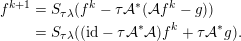 $$\begin{eqnarray}\displaystyle f^{k+1} & = & \displaystyle S_{\unicode[STIX]{x1D70F}\unicode[STIX]{x1D706}}(f^{k}-\unicode[STIX]{x1D70F}{\mathcal{A}}^{\ast }({\mathcal{A}}f^{k}-g))\nonumber\\ \displaystyle & = & \displaystyle S_{\unicode[STIX]{x1D70F}\unicode[STIX]{x1D706}}((\text{id}-\unicode[STIX]{x1D70F}{\mathcal{A}}^{\ast }{\mathcal{A}})f^{k}+\unicode[STIX]{x1D70F}{\mathcal{A}}^{\ast }g).\end{eqnarray}$$
A.4 Alternating direction method of multipliers (ADMM)
Consider solving (A.1) as a constrained problem,
making use of the augmented Lagrangian with dual (adjoint) variable
 $u$
,
$u$
,
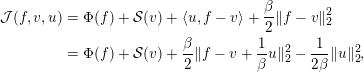 $$\begin{eqnarray}\displaystyle {\mathcal{J}}(f,v,u) & = & \displaystyle \unicode[STIX]{x1D6F7}(f)+{\mathcal{S}}(v)+\langle u,f-v\rangle +\frac{\unicode[STIX]{x1D6FD}}{2}\Vert f-v\Vert _{2}^{2}\nonumber\\ \displaystyle & = & \displaystyle \unicode[STIX]{x1D6F7}(f)+{\mathcal{S}}(v)+\frac{\unicode[STIX]{x1D6FD}}{2}\Vert f-v+\frac{1}{\unicode[STIX]{x1D6FD}}u\Vert _{2}^{2}-\frac{1}{2\unicode[STIX]{x1D6FD}}\Vert u\Vert _{2}^{2},\end{eqnarray}$$
which results in the sequential update sequence
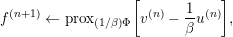 $$\begin{eqnarray}\displaystyle & \displaystyle f^{(n+1)}\leftarrow \operatorname{prox}_{(1/\unicode[STIX]{x1D6FD})\unicode[STIX]{x1D6F7}}\biggl[v^{(n)}-\frac{1}{\unicode[STIX]{x1D6FD}}u^{(n)}\biggr], & \displaystyle\end{eqnarray}$$
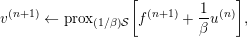 $$\begin{eqnarray}\displaystyle & \displaystyle v^{(n+1)}\leftarrow \operatorname{prox}_{(1/\unicode[STIX]{x1D6FD}){\mathcal{S}}}\biggl[f^{(n+1)}+\frac{1}{\unicode[STIX]{x1D6FD}}u^{(n)}\biggr], & \displaystyle\end{eqnarray}$$
 $$\begin{eqnarray}\displaystyle & \displaystyle u^{(n+1)}\leftarrow u^{(n)}+\unicode[STIX]{x1D6FD}(f^{(n+1)}-v^{(n+1)}). & \displaystyle\end{eqnarray}$$
B. The Wasserstein
$1$
-distance

Let
 $X$
be a measurable separable Banach space and
$X$
be a measurable separable Banach space and
 $\mathscr{P}_{X}$
the space of probability measures on
$\mathscr{P}_{X}$
the space of probability measures on
 $X$
. The Wasserstein 1-distance
$X$
. The Wasserstein 1-distance
 ${\mathcal{W}}:\mathscr{P}_{X}\times \mathscr{P}_{X}\rightarrow \mathbb{R}$
is a metric on
${\mathcal{W}}:\mathscr{P}_{X}\times \mathscr{P}_{X}\rightarrow \mathbb{R}$
is a metric on
 $\mathscr{P}_{X}$
that can be defined as (Villani Reference Villani2009, Definition 6.1)
$\mathscr{P}_{X}$
that can be defined as (Villani Reference Villani2009, Definition 6.1)
 $$\begin{eqnarray}{\mathcal{W}}(p,q):=\inf _{\unicode[STIX]{x1D707}\in \unicode[STIX]{x1D6F1}(p,q)}\mathbb{E}_{(\unicode[STIX]{x1D557},\unicode[STIX]{x1D559})\sim \unicode[STIX]{x1D707}}[\Vert \unicode[STIX]{x1D557}-\unicode[STIX]{x1D559}\Vert _{X}]\quad \text{for }p,q\in \mathscr{P}_{X}.\end{eqnarray}$$
In the above,
 $\unicode[STIX]{x1D6F1}(p,q)\subset \mathscr{P}_{X\times X}$
denotes the family of joint probability measures on
$\unicode[STIX]{x1D6F1}(p,q)\subset \mathscr{P}_{X\times X}$
denotes the family of joint probability measures on
 $X\times X$
that has
$X\times X$
that has
 $p$
and
$p$
and
 $q$
as marginals. Note also that we assume
$q$
as marginals. Note also that we assume
 $\mathscr{P}_{X}$
only contains measures where the Wasserstein distance takes finite values (Wasserstein space): see Villani (Reference Villani2009, Definition 6.4) for the formal definition.
$\mathscr{P}_{X}$
only contains measures where the Wasserstein distance takes finite values (Wasserstein space): see Villani (Reference Villani2009, Definition 6.4) for the formal definition.
The Wasserstein 1-distance in (B.1) can be rewritten using the Kantorovich–Rubinstein dual characterization (Villani Reference Villani2009, Remark 6.5, p. 95), resulting in
 $$\begin{eqnarray}{\mathcal{W}}(p,q)=\sup _{\substack{ \operatorname{D}:X\rightarrow \mathbb{R}\,\,\, \\ \operatorname{D}\in \operatorname{Lip}(X)}}\{\mathbb{E}_{\unicode[STIX]{x1D557}\sim q}[\operatorname{D}(\unicode[STIX]{x1D557})]-\mathbb{E}_{\unicode[STIX]{x1D559}\sim p}[\operatorname{D}(\unicode[STIX]{x1D559})]\}\quad \text{for }p,q\in \mathscr{P}_{X}.\end{eqnarray}$$
Here,
 $\operatorname{Lip}(X)$
denotes real-valued 1-Lipschitz maps on
$\operatorname{Lip}(X)$
denotes real-valued 1-Lipschitz maps on
 $X$
, that is,
$X$
, that is,
The above constraint can be hard to enforce in (B.2) as is, so following Gulrajani et al. (Reference Gulrajani, Ahmed, Arjovsky, Dumoulin, Courville and Guyon2017) and Adler and Lunz (Reference Adler, Lunz and Bengio2018) we prefer the gradient characterization
 $$\begin{eqnarray}\operatorname{D}\in \operatorname{Lip}(X)~\Longleftrightarrow ~\Vert \unicode[STIX]{x2202}\!\operatorname{D}(f)\Vert _{X^{\ast }}\leq 1\quad \text{for all }f\in X,\end{eqnarray}$$
where
 $\unicode[STIX]{x2202}$
indicates the Fréchet derivative and
$\unicode[STIX]{x2202}$
indicates the Fréchet derivative and
 $X^{\ast }$
is the dual space of
$X^{\ast }$
is the dual space of
 $X$
. In our setting,
$X$
. In our setting,
 $X$
is an
$X$
is an
 $L_{2}$
-space, which is a Hilbert space so
$L_{2}$
-space, which is a Hilbert space so
 $X^{\ast }=X$
, and the Fréchet derivative becomes the (Hilbert space) gradient of
$X^{\ast }=X$
, and the Fréchet derivative becomes the (Hilbert space) gradient of
 $\operatorname{D}$
.
$\operatorname{D}$
.


 Open access