

1. Introduction
Markov processes are important modeling tools that help researchers describe real-world phenomena. Thus, it comes as no surprise that the Erlang-A model, which is a Markovian and multiserver queueing model that incorporates customer abandonments, is an important modeling tool in a multitude of application settings. Some of the more prominent applications include telecommunications and call/contact centers, healthcare, urban mobility and transportation, and more recently cloud computing; see, for example, [Reference Mandelbaum28], [Reference Massey29], [Reference Yom-Tov and Mandelbaum45], [Reference Pender and Phung-Duc37], [Reference Boxma and de Waal3], [Reference Brown5], [Reference Garnett, Mandelbaum and Reiman13], [Reference Zohar, Mandelbaum and Shimkin48], [Reference Whitt44], [Reference Borst, Mandelbaum and Reiman2], [Reference van Leeuwaarden and Knessl41], [Reference Knessl and van Leeuwaarden20], [Reference Ward and Glynn42], [Reference Fralix12], and [Reference Braverman, Dai and Feng4]. A detailed overview of the model can be found in [Reference Mandelbaum and Zeltyn26]. There is also a large body of work on non-Markovian abandonment models, such as [Reference Zeltyn and Mandelbaum46], [Reference Mandelbaum and Zeltyn25], [Reference Baccelli, Hebuterne and Kylstra1], [Reference Shimkin and Mandelbaum39], [Reference Ward and Glynn43], and [Reference Reed and Ward38], and the references therein. Despite its importance in many different applications and the well-established history of study regarding customer impatience [Reference Palm34], the Erlang-A queueing model has remained very difficult to analyze and understand. Even analysis of its moments beyond the fourth moment has remained an important topic for additional study.
It is well known that the stationary setting of the Erlang-A queue is much easier to analyze than its nonstationary counterpart [Reference Feldman, Mandelbaum, Massey and Whitt10]. Asymptotic methods, such as heavy traffic limit theory and strong approximations theory, are common approaches for analyzing nonstationary and state-dependent queueing models; see, for example, [Reference Halfin and Whitt16], [Reference Mandelbaum, Massey and Reiman27], [Reference Talreja and Whitt40], [Reference Dong, Feldman and Yom-Tov7], and [Reference Gurvich, Huang and Mandelbaum14]. Uniform acceleration is extremely useful for approximating the transition probabilities and moments, such as the mean and variance of Markov processes. Moreover, the strong approximation methods are useful for analyzing the sample path behavior of the Markov process by showing that the sample paths of properly rescaled queueing processes converge to deterministic dynamical systems and Gaussian process limits.
There are however two main drawbacks of these asymptotic methods. The first is that the method is asymptotic as a function of the model parameters and the results really only hold when the rates are large. Thus, the quality of the approximations significantly depend on the size of the model parameters, and these asymptotic methods have been shown to be quite inaccurate for moderate sized model parameter settings; see, for example, [Reference Massey and Pender30]. The second main drawback is that the asymptotic methods do not generate any important insights for the moments or cumulant moments beyond order two since the limits are based on Brownian motion. Since Brownian motion has symmetry, its cumulants are all zero beyond the second order. Thus, symmetric Brownian approximations are limited in their power to capture asymmetries in higher moments or even the dynamics of the moment generating function, cumulant generating function, or Fourier transform. Moreover, it has been recently shown in [Reference Engblom and Pender9] and [Reference Pender35] that the Erlang-A queue and its variants have nontrivial amounts of skewness and excess kurtosis, which implies that the Erlang-A models are clearly not Gaussian for moderate sized queues. These results also demonstrate that it is important to capture the behavior of the Erlang-A model beyond its second moment as this information can be used in staffing decisions [Reference Massey and Pender31] and [Reference Zhang, Van Leeuwaarden and Zwart47].
One common approximation method that is used in the stochastic networks, queueing, and chemical reactions literature is a moment closure approximation. Moment closure approximations are used to approximate the moments of the queueing process with a surrogate distribution. Often, the set of moment equations for a large number of queueing models is not closed; see, for example, [Reference Matis and Feldman32]. Thus, the closure approximation helps approximate the moments with a closed system using the surrogate distribution. One such method used by Massey and Pender [Reference Massey and Pender30], [Reference Pender49] used Hermite polynomials for approximating the distribution of the queue length process. In fact, they showed that using a quadratic polynomial works quite well. Since the Hermite polynomials are orthogonal to the Gaussian distribution, which has support on the entire real line, these Hermite polynomial approximations do not take into account the discreteness of the queueing process nor do they account for the nonnegativity of the queueing process. However, they showed that Hermite polynomials are natural to analyze since they are orthogonal with respect to the Gaussian distribution and the heavy traffic limits of multiserver queues are Gaussian. In this paper we perform an in-depth analysis of the moments and the moment generating function of the nonstationary Erlang-A queue. As the Erlang-B and Erlang-C queueing models are special cases of the Erlang-A model, we obtain similar results for these models. In a manner similar to what was observed for peer-to-peer networks in [Reference Ferragut and Paganini11], we show that this novel representation allows us to view our bounds and approximations in a new way.
1.1. Main contributions of the paper
The main contributions of this work can be summarized as follows.
We provide new approximations for the moments, moment generating function, and cumulant generating function for the nonstationary Erlang-A queue exploiting the FKG and Jensen’s inequalities.
We derive a novel stochastic interpretation and representation of our approximations as shifted Poisson random variables or M/M/∞ queues, depending on the context. This sheds new light on the complexity of queues in heavy traffic or critically loaded regimes.
We prove precise error bounds for our approximations and we also prove new upper and lower bounds for the nonstationary Erlang-A queue that become exact in certain parameter settings.
1.2. Organization of the paper
The remainder of this paper is organized as follows. In Section 2 we introduce the nonstationary Erlang-A queueing model and its importance in stochastic network theory. In Section 3 we provide approximations for the moments of the Erlang-A system and bound the true values. In Section 4 we derive approximations for the moment generating function of the Erlang-A queue and find stochastic representations for these approximations. We demonstrate these results through several numerical illustrations. We conclude in Section 5.
2. The Erlang-A queueing model
The Erlang-A queueing model is a fundamental queueing model in the stochastic processes literature. The work of Mandelbaum et al. [Reference Mandelbaum, Massey and Reiman27] shows that the queue length process for an M(t)/M/c + M queueing system Q ≡ {Q(t) | t ≥ 0} is represented by the stochastic, time-changed integral equation
 $$Q(t) = Q(0) + {\Pi _1}(\int_0^t \lambda (s){\kern 1pt} {\rm{d}}s) - {\Pi _2}(\int_0^t \mu (Q(s) \wedge c){\kern 1pt} {\rm{d}}s) - {\Pi _3}(\int_0^t \; \theta {(Q(s) - c)^ + }{\kern 1pt} {\rm{d}}s),$$
where Πi ≡ {Πi(t) | t ≥ 0}, for i = 1,2,3, are independent and identically distributed (i.i.d.) standard (rate-1) Poisson processes and (xΛy) = min{x, y}. Thus, we can write the sample path dynamics of the Erlang-A queueing process in terms of three independent unit-rate Poisson processes. A deterministic time change for Π1 transforms it into a nonhomogeneous Poisson arrival process with rate λ(t) that counts the customer arrivals that occurred in the time interval [0,t). A random time change for the Poisson process Π2 gives a departure process that counts the number of serviced customers. We implicitly assume that the number of servers is  $c \in {{\Bbb Z}^ + }$ and that each server works at rate μ. Finally, the random time change of Π3 gives a counting process for the number of customers that abandon the system before beginning service. We also assume that the abandonment distribution is exponential and the rate of abandonments is equal to θ.
One of the main reasons that the Erlang-A queueing model has been so extensively analyzed is that several important queueing models are special cases of it. One special case is the infinite server queue. The infinite-server queue can be derived from the Erlang-A queue in two ways. The first way is to set the number of servers to ∞. This precludes any abandonments since the abandonment rate θ(Q(t) – c)+ is always equal to 0 when the number of servers is infinite. The second way to derive the infinite-server queue is to set the service rate μ equal to the abandonment rate θ. When μ = θ, this implies that the sum of the service and abandonment departure processes is equal to a linear function, i.e. μ(Q(t) Λ c) + θ(Q(t) − c)+ = μQ(t) = θQ(t). Thus, the Erlang-A queueing model becomes an infinite-server queue.
A key insight from [Reference Halfin and Whitt16] is that, for multiserver queueing systems, it is natural to scale up the arrival rate and the number of servers simultaneously. This scaling—known as the Halfin–Whitt scaling—has been an important technique for modeling call centers in the queueing literature. Since the M(t)/M/c + M queueing process is a special case of a single node Markovian service network, we can also construct an associated, uniformly accelerated queueing process where both the new arrival rate ηλ(t) and the new number of servers ηc are scaled by the same factor η > 0. Thus, using the Halfin-Whitt scaling for the Erlang-A model, we arrive at the following sample path representation for the queue length process:
 $$\eqalign{ {Q^\eta }(t) & = {Q^\eta }(0) + {\Pi _1}(\int_0^t \eta \cdot \lambda (s) {\rm{d}}s) - {\Pi _2}(\int_0^t \mu \cdot ({Q^\eta }(s) \wedge \eta \cdot c){\rm{d}}s) \cr & \quad - {\Pi _3}(\int_0^t \theta \cdot {({Q^\eta }(s) - \eta \cdot c)^ + }{\rm{d}}s) \cr & = {Q^\eta }(0) + {\Pi _1}(\int_0^t \eta \cdot \lambda (s) {\rm{d}}s) - {\Pi _2}(\int_0^t \eta \cdot \mu \cdot ({{{Q^\eta }(s)} \over \eta } \wedge c) {\rm{d}}s) \cr & \quad - {\Pi _3}(\int_0^t \eta \cdot \theta \cdot {({{{Q^\eta }(s)} \over \eta } - c)^ + } {\rm{d}}s).} $$
The Halfin-Whitt scaling is defined by simultaneously scaling up the rate of customer demand (which is the arrival rate) with the number of servers. In the context of call centers this is scaling up the number of customers and scaling up the number of agents to answer the phones. In the context of hospitals or healthcare this might be scaling up the number of patients with the number of beds or nurses. Taking the following limits gives us the fluid models of [Reference Mandelbaum, Massey and Reiman27], i.e.
 $$\mathop {\lim }\limits_{\eta \to \infty } {1 \over \eta }{Q^\eta }(t) = q(t)\quad {\rm{almost surely(a}}{\rm{.s}}{\rm{.)}}$$
where the deterministic process q(t), the fluid mean, is governed by the one-dimensional ordinary differential equation (ODE)
 $$\mathop q\limits^ \bullet (t) = \lambda (t) - \mu (q(t) \wedge c) - \theta {(q(t) - c)^ + }.$$
(1)
$$\mathop q\limits^ \bullet (t) = \lambda (t) - \mu (q(t) \wedge c) - \theta {(q(t) - c)^ + }.$$
(1)
Moreover, if we take a diffusion limit, i.e.
 $$\mathop {\lim }\limits_{\eta \to \infty } \sqrt \eta ({1 \over \eta }{Q^\eta }(t) - q(t)) \Rightarrow \tilde Q(t),$$
we get a diffusion process where the variance of the diffusion is given by the following ODE:
 $$\displaylines{ \mathop {\mathop {{\rm{v}}ar}\nolimits}\limits^ \bullet [\tilde Q(t)] = \lambda (t) + \mu \cdot (q(t) \wedge c) + \theta \cdot {(q(t) - c)^ + } - 2 \cdot {\rm{v}}ar[\tilde Q(t)] \cdot (\mu \cdot \{ q(t) < c\} \cr + \theta \cdot \{ q(t) \ge c\} ).} $$
2.1. Mean-field approximation is identical to the fluid limit
In addition to using strong approximations to analyze the queue length process one can also use the functional Kolmogorov forward equations, as outlined in [Reference Massey and Pender30]. The functional forward equations for the Erlang-A model are derived as
 $$\eqalign{ \mathop {\mathbb E}\limits^ \bullet [f(Q(t))] & \equiv \frac{{\text{d}}}{{{\text{d}}t}}{\mathbb E}[f(Q(t))|Q(0) = q(0)] \cr & = \lambda (t){\mathbb E}[f(Q(t) + 1) - f(Q(t))] + {\mathbb E}[\delta (Q(t),c)({\kern 1pt} f(Q(t) - 1) - f(Q(t)))]} $$
(2)
$$\eqalign{ \mathop {\mathbb E}\limits^ \bullet [f(Q(t))] & \equiv \frac{{\text{d}}}{{{\text{d}}t}}{\mathbb E}[f(Q(t))|Q(0) = q(0)] \cr & = \lambda (t){\mathbb E}[f(Q(t) + 1) - f(Q(t))] + {\mathbb E}[\delta (Q(t),c)({\kern 1pt} f(Q(t) - 1) - f(Q(t)))]} $$
(2)
for all appropriate functions f and where δ(Q(t), c) = μ(Q(t) Λ c) + θ(Q(t) − c)+. For the special case in which f(x) = x, we can derive an ODE for the mean queue length process as
 $$\mathop {\mathbb E}\limits^ \bullet [Q(t)] = \lambda (t) - \mu {\mathbb E}[(Q(t) \wedge c)] - \theta {\mathbb E}[(Q(t) - c{)^ + }].$$
(3)
$$\mathop {\mathbb E}\limits^ \bullet [Q(t)] = \lambda (t) - \mu {\mathbb E}[(Q(t) \wedge c)] - \theta {\mathbb E}[(Q(t) - c{)^ + }].$$
(3)
The first thing to note is that this equation is not autonomous and we need to know the distribution of Q(t) a priori in order to compute the expectations on the right-hand side of (3). To know the distribution a priori is impossible except in some special cases like the infinite-server setting. However, it is easy to derive simple approximations for the mean queue length by making some assumptions on the queue length process. This is known as a closure approximation and one common closure approximation method is to simply take the expectations from outside the function to inside the function. This implies that the expectation  ${\mathbb E}[f(X)]$ becomes $f({\mathbb E}[X])$. This method is known as a mean-field approximation in physics and is also known as the deterministic mean approximation in [Reference Massey and Pender30]. By applying the mean-field approximation to (3), we can show that the resulting differential equation is given by the following autonomous ODE:
 $$\mathop {\mathbb E}\limits^ \bullet [{Q_{\text{f}}}(t)] = \lambda (t) - \mu ({\mathbb E}[{Q_{\text{f}}}] \wedge c) - \theta {({\mathbb E}[{Q_{\text{f}}}] - c)^ + }.$$
(4)
$$\mathop {\mathbb E}\limits^ \bullet [{Q_{\text{f}}}(t)] = \lambda (t) - \mu ({\mathbb E}[{Q_{\text{f}}}] \wedge c) - \theta {({\mathbb E}[{Q_{\text{f}}}] - c)^ + }.$$
(4)
By careful inspection, we can observe that the ODE given by the mean-field approximation is identical to the fluid limit of (1). Moreover, if we simulate the queueing process and compare it to the mean-field limit, we notice an ordering property. For example, in Figure 1(a), we simulate the Erlang-A queue and compare it to the fluid model. We observe that, when θ < μ, the simulated mean is larger than the fluid mean. This is precisely what our results predict. Moreover, in Figure 1(b), we simulate the Erlang-A queue and compare it to the fluid model when θ > μ and observe that the simulated queue length is smaller than the fluid limit.
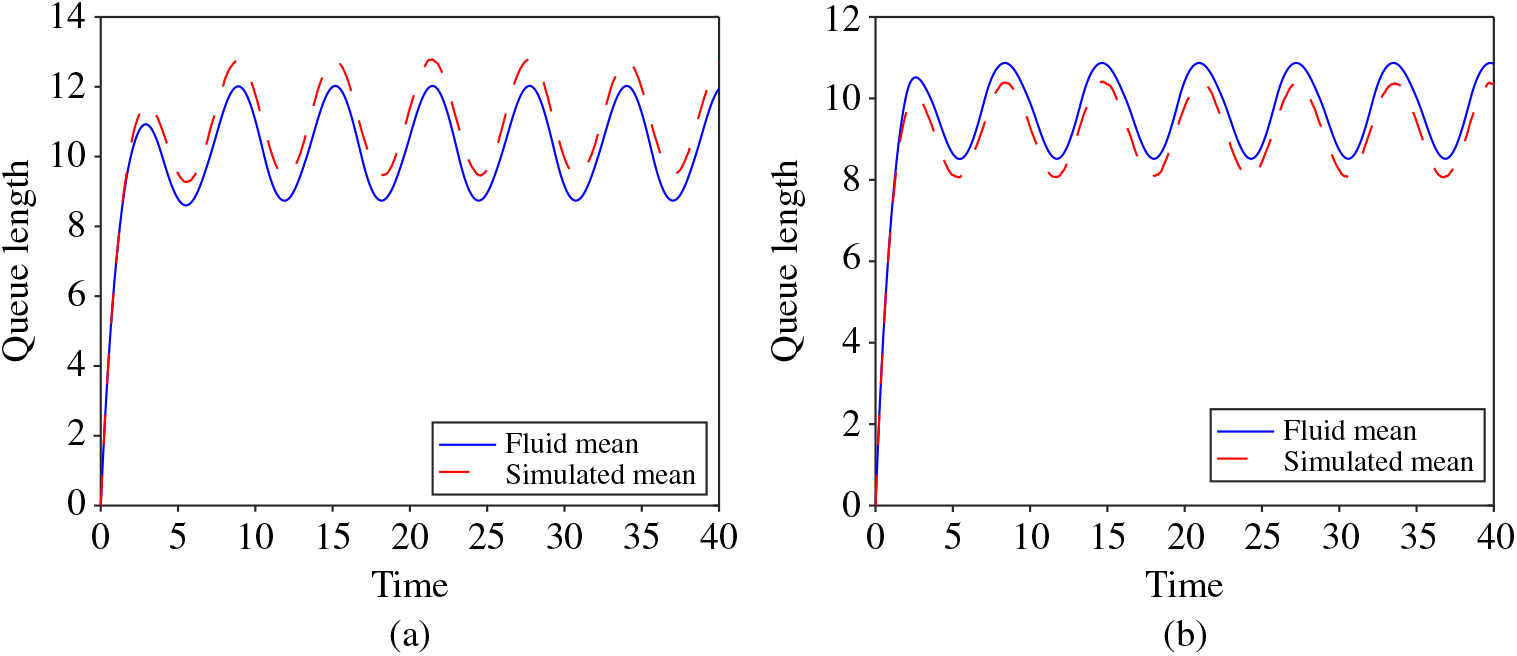
Figure 1. Comparison of a simulated Erlang-A queue and fluid model for λ(t) = 10 + 2 sin(t), μ = 1, Q(0) = 0, c = 10, and (a) θ = 0.5 and (b) θ = 2.
Our goal in this work is to explain the behavior that we observe in Figure 1, which we will do in the following section. Before concluding our overview of the Erlang-A queueing model, we make a brief remark for notational clarity.
Remark 1
Throughout the remainder of this work, we use Q(t) to represent the true queueing process and Q f(t) to represent the fluid approximation of it. This fluid approximation is a stochastic process that will be fully described in this work. In fact, in Section 4 we characterize the fluid approximations and use insight from these representations to bound the true queue length from above and below.
3. Inequalities for the moments of the Erlang-A queue
In this section we prove conditions under which the true moments of the Erlang-A queue either dominate their corresponding fluid limits or are dominated by them. We find that the relationship between the service rate and the abandonment rate determines whether or not the moments of the Erlang-A queue are dominated by the associated fluid limits. The remainder of this section is organized as follows. In Subsection 3.1 we derive inequalities for the true mean of the Erlang-A and its fluid approximation. In Subsection 3.2 we extend these inequalities to analogous results for the mth moment of the queueing system. Finally, in Subsection 3.3 we provide figures from numerical experiments that validate our theoretical results.
3.1. Inequalities for the mean
We begin with analysis of the mean of the Erlang-A queue. While we will generalize to all higher moments in Subsection 3.2, we first provide the mean result separately to give the reader the essence and elegance of our result. Before we proceed, we first establish a lemma for comparisons of ordinary differential equations that will be fundamental for our subsequent analysis.
Lemma 1
(A comparison lemma.) Let f: ${{\mathbb R}^2} \to {\mathbb R}$ be a continuous function in both variables. If we assume that the initial value problem
 $$\mathop x\limits^ \bullet (t) = f(t,x(t)),\quad \quad x(0) = {x_0},$$
has a unique solution for the time interval [0,T] and
 $$\mathop y\limits^ \bullet (t) \le f(t,y(t))\quad {\rm{for }}t \in [0,T]\,and\,y(0) \le {x_0},$$
then x(t) ≥ y(t) for all t ∈ [0,T].
Proof. The proof of this result is given in [Reference Hale and Verduyn Lunel15].
With this lemma in hand, we can now derive relationships for the fluid limit and the true mean. As seen in the proof of Theorem 1 below, this result follows from the application of Lemma 1 and the convexity seen in the fluid approximation.
Theorem 1
For the Erlang-A queue, if Q(0) = Q f(0) then the true mean dominates the fluid limit when θ < μ, the fluid limit dominates the true mean when θ > μ, and the two means are equal when θ = μ.
Proof. Recall from (3) that the true mean satisfies the differential equation
 $$\mathop {\mathbb E}\limits^ \bullet [Q(t)] = \lambda (t) - \mu {\mathbb E}[(Q \wedge c)] - \theta {\mathbb E}[(Q - c{)^ + }],$$
and from (4) the fluid limit satisfies the differential equation
 $$\mathop {\mathbb E}\limits^ \bullet [{Q_{\text{f}}}(t)] = \lambda (t) - \mu ({\mathbb E}[{Q_{\text{f}}}] \wedge c) - \theta {({\mathbb E}[{Q_{\text{f}}}] - c)^ + }.$$
We can simplify both equations by observing that (X Λ c)+ (X − c) + = X for any random variable X. Thus, we have the following two equations for the true mean and the fluid limit:
 $$\displaylines{ \mathop {\mathbb E}\limits^ \bullet [Q(t)] = \lambda (t) - \theta E[Q] + (\theta - \mu ){\mathbb E}[(Q \wedge c)], \cr \mathop {\mathbb E}\limits^ \bullet [{Q_{\text{f}}}(t)] = \lambda (t) - \theta {\mathbb E}[{Q_{\text{f}}}] + (\theta - \mu )({\mathbb E}[{Q_{\text{f}}}] \wedge c). \cr} $$
If we take the difference of the two equations, we obtain
 $$\mathop {\mathbb E}\limits^ \bullet [Q(t)] - \mathop {\mathbb E}\limits^ \bullet [{Q_{\text{f}}}(t)] = \theta ({\mathbb E}[{Q_{\text{f}}}] - {\mathbb E}[Q]) + (\theta - \mu )({\mathbb E}[(Q \wedge c)] - ({\mathbb E}[{Q_{\text{f}}}] \wedge c)).$$
Now since the minimum function (Q Λ c) is a concave function, we have
 $$({\mathbb E}[(Q \wedge c)] - ({\mathbb E}[Q] \wedge c)) \le 0$$
for any random variable Q. Thus, by Lemma 1, we have, for θ < μ,
 $${\mathbb E}[Q(t)] - {\mathbb E}[{Q_{\text{f}}}(t)] \ge 0$$
and, for θ > μ,
 $${\mathbb E}[Q(t)] - {\mathbb E}[{Q_{\text{f}}}(t)] \le 0.$$
Finally, for θ = μ, we have
 $${\mathbb E}[Q(t)] - {\mathbb E}[{Q_{\text{f}}}(t)] = 0$$
since both differential equations are initialized with the same value and the origin is an equilibrium point for the difference.
As discussed in Section 2, the Erlang-A model is quite versatile in its relation to other queueing systems of practical interest. In the two following corollaries, we find that Theorem 1 can be applied to the Erlang-B and Erlang-C models.
Corollary 1
For the Erlang-B queueing model, if Q(0) = Q f(0) then  ${\mathbb E}[Q(t)] \le {\mathbb E}\left[ {{Q_{\text{f}}}(t)} \right]$ for all t ≥ 0.
Proof. This is obvious after noting that the Erlang-B queue is a limit of the Erlang-A queue by letting θ → ∞.
Corollary 2
For the Erlang-C queueing model, if Q(0) = Q f(0) then  ${\mathbb E}[Q(t)] \ge {\mathbb E}\left[ {{Q_{\text{f}}}(t)} \right]$ for all t ≥ 0.
Proof. This is obvious after noting that the Erlang-C queue is an Erlang-A queue with θ = 0. Since μ is assumed to be positive, we fall into the case where θ < μ and this completes the proof.
Remark 2
Given that we use Jensen’s inequality and the FKG inequality later in the paper, we consider itr important to differentiate them. Here we give an example that sets the two apart. If we have the following function Q n then Jensen’s inequality implies that  ${\mathbb E}[{Q^n}] \ge {\mathbb E}{[Q]^n}$. However, the FKG inequality implies that ${\mathbb E}[{Q^n}] \ge {\mathbb E}[{Q^{n - 1}}]{\mathbb E}[Q]$. We note that, by iterating the FKG inequality n-2 more times, it yields Jensen’s inequality for the moments of random variables.
3.2. Inequalities for the mth moment
In this subsection we extend the previous findings for the mean to higher moments of the queueing system. Like the result for the mean, this is again built through observation of the convexity in the differential equation of the fluid approximation.
Theorem 2
For the Erlang-A queue,  $m \in {{\Bbb Z}^ + }$, and t ≥ 0, if Q(0) = Q f(0) then ${\rm{E}}[{Q^m}(t)] \ge {\rm{E}}[Q_{\rm{f}}^m(t)]$ when θ < μ, ${\rm{E}}[{Q^m}(t)] \le {\rm{E}}[Q_{\rm{f}}^m(t)]$ when θ > μ, and ${\rm{E}}[{Q^m}(t)] = {\rm{E}}[Q_{\rm{f}}^m(t)]$ when θ = μ.
Proof. We will use proof by induction. For the base case, we can apply Theorem 1. Now, suppose that the statement holds for j ∈ {1,2,…,m-1}. By (2) and expansion through the binomial theorem, we note that the mth moment satisfies the differential equation
 $$\eqalign{ & \mathop {\mathbb E}\limits^ \bullet [{Q^m}(t)] \cr & \quad \quad = \lambda (t){\text{E}} \left[\sum\limits_{j = 0}^m \left( {\matrix m \\ j } \right){Q^j}(t) - {Q^m}(t) \right] \cr & \quad \quad \quad + {\text{E}} \left[(\sum\limits_{j = 0}^m \left( {\matrix m \\ j} \right){( - 1)^{m - j}}{Q^j}(t) - {Q^m}(t))(\theta Q(t) - (\theta - \mu )(Q(t) \wedge c)) \right] \cr & \quad \quad = \lambda (t)\sum\limits_{j = 0}^{m - 1} \left( {\matrix m \\ j } \right){\text{E}}[{Q^j}(t)] + \theta \sum\limits_{j = 0}^{m - 1} \left( {\matrix m \\ j} \right){( - 1)^{m - j}}{\text{E}}[{Q^{j + 1}}(t) ] \cr & \quad \quad \quad + (\theta - \mu ){\mathbb E} \left[(\sum\limits_{j = 0}^{m - 1} \left( {\matrix m \\ j } \right){( - 1)^{m - 1 - j}}{Q^{j + 1}}(t)) \wedge (c\sum\limits_{j = 0}^{m - 1} \left( {\matrix m \\ j} \right){( - 1)^{m - 1 - j}}{Q^j}(t)) \right],} $$
whereas the approximate autonomous version satisfies
 $$\eqalign{& \mathop {\mathbb E}\limits^ \bullet [Q_{\text{f}}^m(t)] \cr & \quad \quad = \lambda (t)\sum\limits_{j = 0}^{m - 1} \left( {\matrix m \\ j} \right){\text{E}}[Q_{\text{f}}^j(t)] + \theta \sum\limits_{j = 0}^{m - 1} \left( {\matrix m \\ j } \right){( - 1)^{m - j}}{\text{E}}[Q_{\text{f}}^{j + 1}(t)] \cr & \quad \quad \quad {\kern 1pt} + (\theta - \mu )\left({\mathbb E}[\sum\limits_{j = 0}^{m - 1} \left( {\matrix m \\ j } \right){( - 1)^{m - 1 - j}}Q_f^{j + 1}(t)] \wedge {\mathbb E}[c\sum\limits_{j = 0}^{m - 1} \left( {\matrix m \\ j} \right){( - 1)^{m - 1 - j}}Q_f^j(t)]\right),} $$
which is the closure approximation of the differential equation for E[Q m(t)]. Now by taking the difference of these ODEs, we have
 \[\begin{array}{l}\mathop {\mathbb E}\limits^ \bullet [{Q^m}(t)] - \mathop {\mathbb E}\limits^ \bullet [Q_{\rm{f}}^m(t)]\\ = \lambda (t)\sum\limits_{j = 0}^{m - 1} {\left( {\begin{array}{*{20}{c}}m\\j\end{array}} \right)} {\rm{E}}[{Q^j}(t) - Q_{\rm{f}}^j(t)] + \theta \sum\limits_{j = 0}^{m - 1} {\left( {\begin{array}{*{20}{c}}m\\j\end{array}} \right)} {( - 1)^{m - j}}{\rm{E}}[{Q^{j + 1}}(t) - Q_{\rm{f}}^{j + 1}(t)]\\ + (\theta - \mu )\left( {{\rm{E}}\left[ {\sum\limits_{j = 0}^{m - 1} {\left( {\begin{array}{*{20}{c}}m\\j\end{array}} \right)} {{( - 1)}^{m - 1 - j}}{Q^{j + 1}}(t)} \right] \wedge \left( {c\sum\limits_{j = 0}^{m - 1} {\left( {\begin{array}{*{20}{c}}m\\j\end{array}} \right)} {{( - 1)}^{m - 1 - j}}Q_f^j(t))} \right]} \right.\\\left. { - {\rm{E}}\left[ {\sum\limits_{j = 0}^{m - 1} {\left( {\begin{array}{*{20}{c}}m\\j\end{array}} \right)} {{( - 1)}^{m - 1 - j}}{Q^{j + 1}}(t)} \right] \wedge {\rm{E}}\left[ {c\sum\limits_{j = 0}^{m - 1} {\left( {\begin{array}{*{20}{c}}m\\j\end{array}} \right)} {{( - 1)}^{m - 1 - j}}Q_f^j(t)} \right]} \right)\end{array}\]
Because the minimum is a concave function, for any X and Y with real means, E[X Λ Y] ≤ E[X] Λ E[Y]. Thus, by Lemma 1, we have, for θ < μ,
 $${\mathbb E}[{Q^m}(t)] - {\mathbb E}[Q_{\text{f}}^m(t)] \ge 0,$$
if θ > μ,
 $${\mathbb E}[{Q^m}(t)] - {\mathbb E}[Q_{\text{f}}^m(t)] \le 0,$$
and if θ = μ,
 $${\mathbb E}[{Q^m}(t)] - {\mathbb E}[Q_{\text{f}}^m(t)] = 0$$
since both differential equations are initialized with the same value, the origin is an equilibrium point for the difference, and all the lower-power terms in the differential equations follow this structure, which we know from the inductive hypothesis. Therefore, we see this holds for m, which completes the proof via Lemma 1.
Again as we have seen for the mean, we can exploit the versatility of the Erlang-A queue to extend these insights to the Erlang-B and Erlang-C models as well.
Corollary 3
For the Erlang-B queueing model, if Q(0) = Q f(0) then  ${\mathbb E}[{Q^m}(t)] \le {\mathbb E}[Q_{\text{f}}^m(t)]$ for all t ≥ 0 and $m \in {{\Bbb Z}^ + }$.
Proof. This is obvious after noting that the Erlang-B queue is a limit of the Erlang-A queue by letting θ→∞.
Corollary 4
For the Erlang-C queueing model, if Q(0) = Q f(0) then  ${\mathbb E}[{Q^m}(t)] \ge {\mathbb E}[Q_{\text{f}}^m(t)]$ for all t ≥ 0 and $m \in {{\Bbb Z}^ + }$.
Proof. This is obvious after noting that the Erlang-C queue is an Erlang-A queue with θ = 0. Since μ is assumed to be positive, we fall into the case where θ < μ and this completes the proof.
3.3. Numerical results
In this subsection we describe numerical results for approximating the moments of the Erlang-A queue and examine them relative to our findings. We do so through Figures 2, 3, 4, and 5. All four of these figures demonstrate the findings of Theorem 2. In Figures 2 and 3 we show the first four moments of the Erlang-A queue and their respective fluid approximations for the θ < μ and θ > μ cases, respectively. In these plots we take the arrival rate at time t ≥ 0 to be λ(t) = 10 + 2 sin(t). We initialize the queue as empty, and we assume that the queueing system has c = 10 servers each with an exponential service rate μ = 1. We test two different cases for the abandonment rate, θ = 0.5 and θ = 2. In these settings we observe that, when θ < μ, the fluid approximations are below their corresponding simulated stochastic values and, when θ > μ, the fluid values are greater than the simulations, and this matches the statements of Theorems 1 and 2.
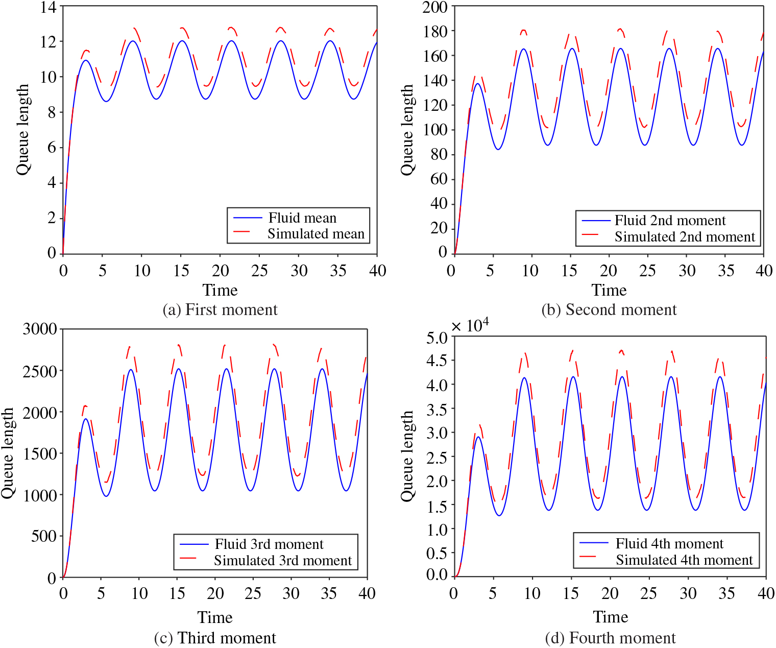
Figure 2. The first four moments of the Erlang-A queue and their respective fluid approximations for λ(t) = 10 + 2 sin(t), μ = 1, θ = 0.5, Q(0) = 0, and c = 10.
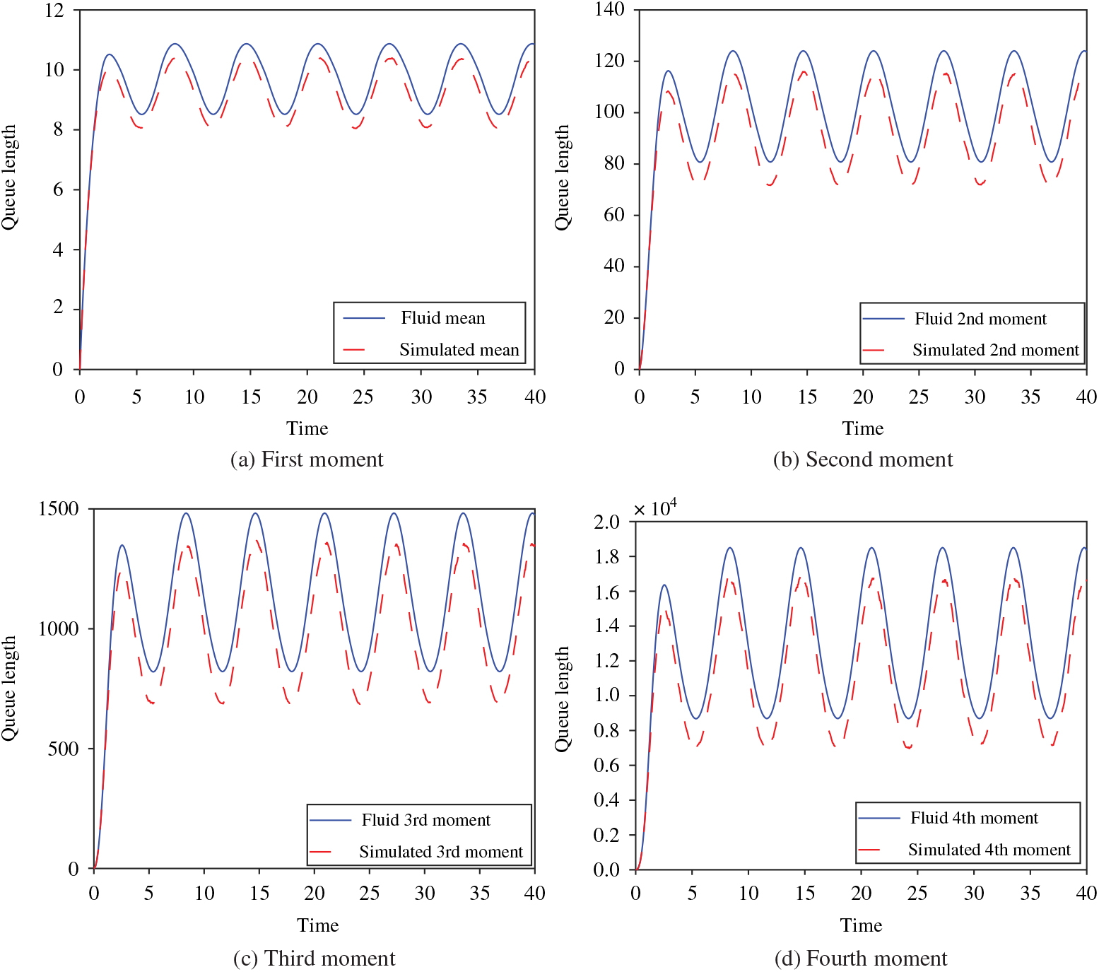
Figure 3. The first four moments of the Erlang-A queue and their respective fluid approximations for λ(t) = 10 + 2 sin(t), μ = 1, θ = 2, Q(0) = 0, and c = 10.
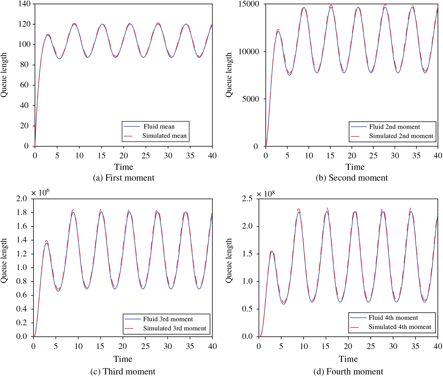
Figure 4. The first four moments of the Erlang-A queue and their respective fluid approximations for λ(t) = 100 + 20 sin(t), μ = 1, θ = 0.5, Q(0) = 0, and c = 100.
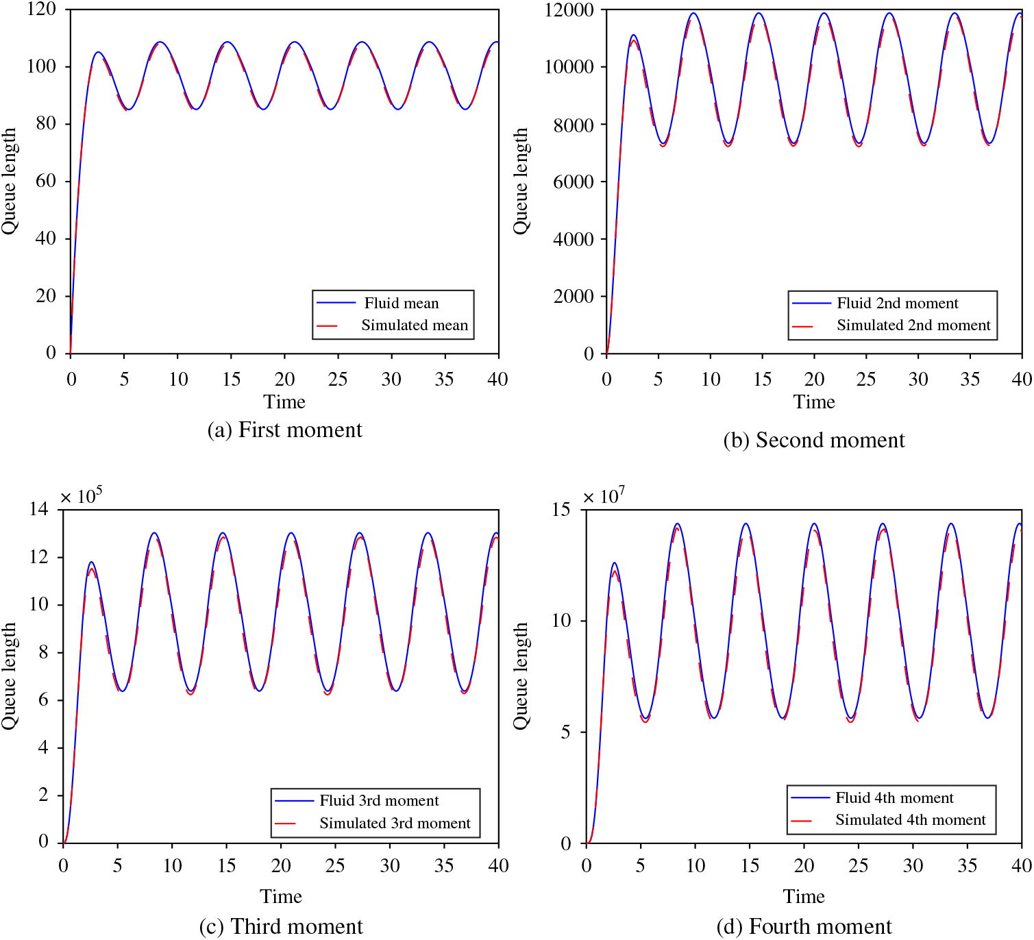
Figure 5. The first four moments of the Erlang-A queue and their respective fluid approximations for λ(t) = 100 + 20 sin(t), μ = 1, θ = 2, Q(0) = 0, and c = 100.
We observe the same relationships in Figures 4 and 5. For both of these figures we set λ(t) = 100 + 20 sin(t) and c = 100, but otherwise use the same values as for Figures 2 and 3. With this increase in the arrival intensity and the number of servers, we see that the gaps between the fluid approximations and the simulations are again present, albeit proportionally smaller and may be most easily observed by inspection at the peaks and valleys of the trigonometric forms.
To gain further insight into the relationship between these moments and their approximations, we now plot the relative error for each moment displayed in the past four parameter settings. Specifically, we define the relative error as
 $${\rm{RE}}(t) = {{|{\rm{E}}[{Q^m}(t)] - {\rm{E}}{\kern 1pt} [Q_f^m(t)]|} \over {{\rm{E}}[{Q^m}(t)]}}.$$
Using empirically calculated moments via simulation and approximations calculated via differential equations, we plot this function across the four settings in Figures 6, 7, 8, and 9. We note that the error appears to become more localized to the valleys of the sine curve as the moments grow higher in power or for λ(t) and c of greater magnitude, whereas the errors of the means when λ(t) and c are not as large (i.e. Figures 6 and 7) oscillate more quickly with the maxima of its relative error occurring between the mean’s extremes. This difference makes sense since at this point the denominator is at its smallest and this will have a more pronounced effect for the larger values at the higher moments. Furthermore, we can also infer that the highest relative error at the mean takes place when the value of the mean is equal to the number of servers, which creates a change in behavior. For more on these phenomena, see [Reference Massey and Pender30] and [Reference Pender35]. Additionally, we observe that as the rate and the number of servers grow large, the approximations appear to be more accurate.
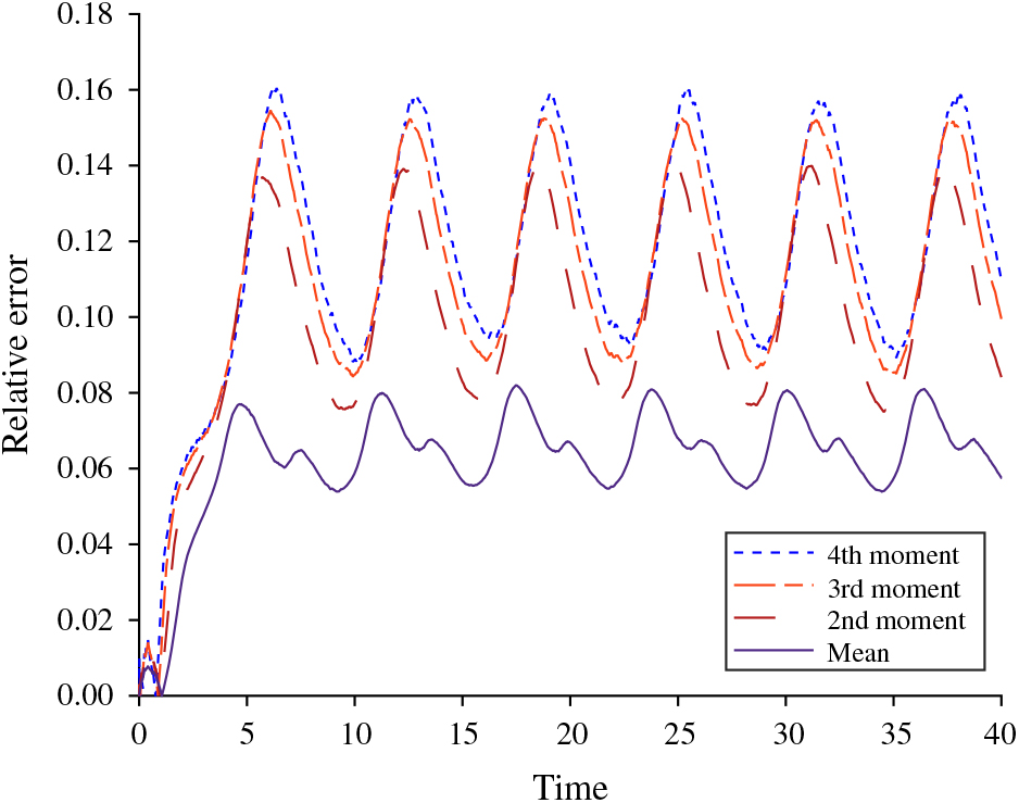
Figure 6. The relative error for λ(t) = 10 + 2 sin(t), μ = 1, θ = 0.5, Q(0) = 1, and c = 10.
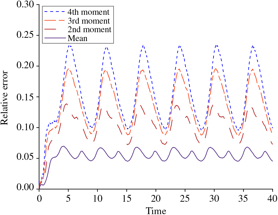
Figure 7. The relative error for λ(t) = 10 + 2 sin(t), μ = 1, θ = 2, Q(0) = 1, and c = 10.
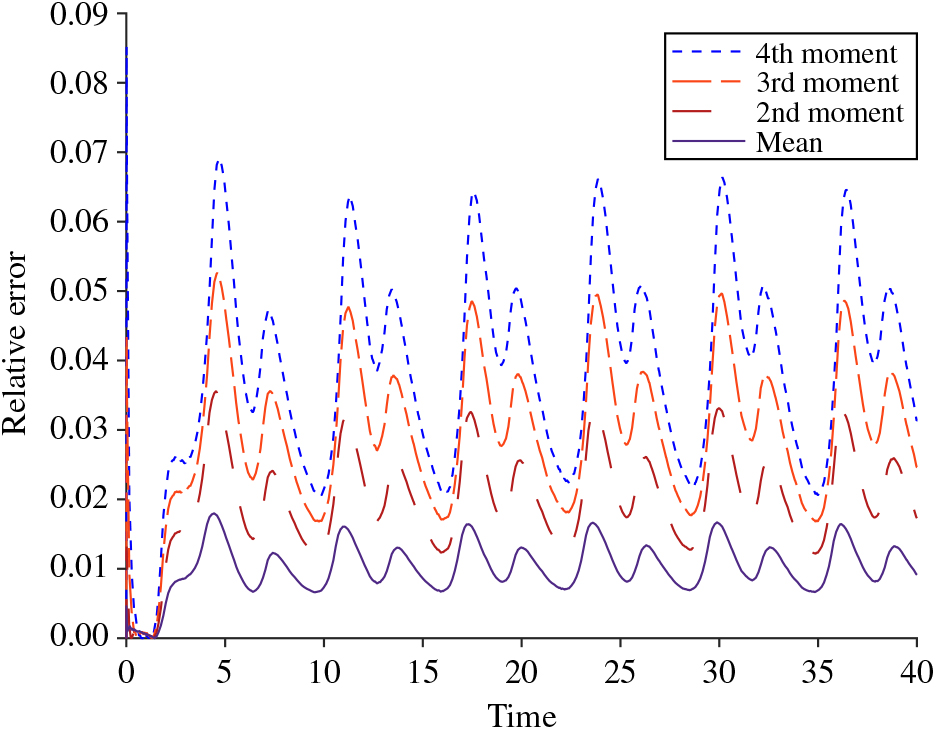
Figure 8. The relative error for λ(t) = 100 + 20 sin(t), μ = 1, θ = 0.5, Q(0) = 1, and c = 100.
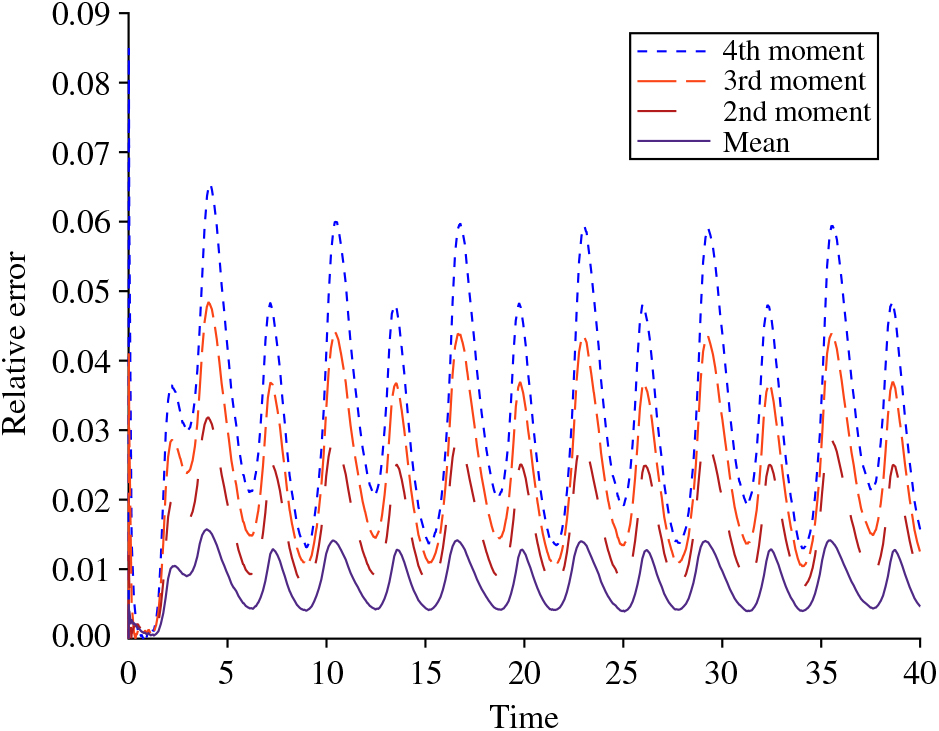
Figure 9. The relative error for λ(t) = 100 + 20 sin(t), μ = 1, θ = 2, Q(0) = 1, and c = 100.
4. Inequalities and characterizations for generating functions of the Erlang-A queue
Building on what we have proved for the moments of the Erlang-A, we can provide similar inequalities for the moment generating function and the cumulant generating function again through convexity in the ordinary or partial differential equations for the fluid approximations. We provide these inequalities in Subsections 4.1 and 4.2, respectively. As a result, we uncover new stochastic representations for our fluid approximations as shifted Poisson random variables. We describe these stochastic representations for systems in steady-state in Subsection 4.3 and for nonstationary systems in Subsection 4.4. We conclude this section with a variety of demonstrations of these results through numerical experiments in Subsection 4.5.
4.1. An inequality for the moment generating function of the Erlang-A queue
Using the functional forward equations as given by (2), we can show that the moment generating function for the Erlang-A queue satisfies the following partial differential equation:
 $$\displaylines{ \mathop {\mathbb E}\limits^ \bullet [{{\text{e}}^{\alpha Q(t)}}] = \lambda (t)({{\text{e}}^\alpha } - 1){\mathbb E}[{{\text{e}}^{\alpha \cdot Q(t)}}] + \theta ({{\text{e}}^{ - \alpha }} - 1) \cdot {\mathbb E}[Q(t){{\text{e}}^{\alpha \cdot Q(t)}}] \cr - (\theta - \mu )({{\text{e}}^{ - \alpha }} - 1){\mathbb E}[(Q(t) \wedge c){{\text{e}}^{\alpha Q(t)}}]. \cr} $$
(5)
$$\displaylines{ \mathop {\mathbb E}\limits^ \bullet [{{\text{e}}^{\alpha Q(t)}}] = \lambda (t)({{\text{e}}^\alpha } - 1){\mathbb E}[{{\text{e}}^{\alpha \cdot Q(t)}}] + \theta ({{\text{e}}^{ - \alpha }} - 1) \cdot {\mathbb E}[Q(t){{\text{e}}^{\alpha \cdot Q(t)}}] \cr - (\theta - \mu )({{\text{e}}^{ - \alpha }} - 1){\mathbb E}[(Q(t) \wedge c){{\text{e}}^{\alpha Q(t)}}]. \cr} $$
(5)
As for the nonautonomous differential equation for the mean in (3), we also cannot directly compute the moment generating function since we do not know the distribution of the queue length a priori. This is also true for numerical purposes. Unless we can compute the expectation that includes the minimum function it is impossible to know the moment generating function, except in special cases such as the infinite-server queue and some cases of the stationary Erlang-B queue. Thus, it is useful to obtain approximations that are explicit upper or lower bounds for the moment generating function. By using Jensen’s inequality for concave functions, we can approximate the moment generating function with the partial differential equation
 $$\eqalign{ \mathop {\mathbb E}\limits^ \bullet [{{\text{e}}^{\alpha {Q_{\text{f}}}(t)}}] & = \lambda (t)({{\text{e}}^\alpha } - 1){\mathbb E}[{{\text{e}}^{\alpha {Q_{\text{f}}}(t)}}] + \theta ({{\text{e}}^{ - \alpha }} - 1){\mathbb E}[{Q_{\text{f}}}(t){{\text{e}}^{\alpha {Q_{\text{f}}}(t)}}] \cr & \quad - (\theta - \mu )({{\text{e}}^{ - \alpha }} - 1)({\mathbb E}[{Q_{\text{f}}}(t){{\text{e}}^{\alpha {Q_{\text{f}}}(t)}}] \wedge {\mathbb E}[c{{\text{e}}^{\alpha \cdot {Q_{\text{f}}}(t)}}]), \cr} $$
(6)
$$\eqalign{ \mathop {\mathbb E}\limits^ \bullet [{{\text{e}}^{\alpha {Q_{\text{f}}}(t)}}] & = \lambda (t)({{\text{e}}^\alpha } - 1){\mathbb E}[{{\text{e}}^{\alpha {Q_{\text{f}}}(t)}}] + \theta ({{\text{e}}^{ - \alpha }} - 1){\mathbb E}[{Q_{\text{f}}}(t){{\text{e}}^{\alpha {Q_{\text{f}}}(t)}}] \cr & \quad - (\theta - \mu )({{\text{e}}^{ - \alpha }} - 1)({\mathbb E}[{Q_{\text{f}}}(t){{\text{e}}^{\alpha {Q_{\text{f}}}(t)}}] \wedge {\mathbb E}[c{{\text{e}}^{\alpha \cdot {Q_{\text{f}}}(t)}}]), \cr} $$
(6)
which, for  ${M_f}(t,\alpha ) \equiv {\rm{E}}{\kern 1pt} [{{\rm{e}}^{\alpha {Q_{\rm{f}}}(t)}}],$ can be expressed as
 $$\eqalign{ {{\partial {M_f}(t,\alpha )} \over {\partial t}} & = \lambda (t)({{\rm{e}}^\alpha } - 1) \cdot {M_f}(t,\alpha ) + \theta ({{\rm{e}}^{ - \alpha }} - 1){{\partial {M_f}(t,\alpha )} \over {\partial \alpha }} \cr & \quad - (\theta - \mu )({{\rm{e}}^{ - \alpha }} - 1)({{\partial {M_f}(t,\alpha )} \over {\partial \alpha }} \wedge c{M_f}(t,\alpha )).} $$
(7)
$$\eqalign{ {{\partial {M_f}(t,\alpha )} \over {\partial t}} & = \lambda (t)({{\rm{e}}^\alpha } - 1) \cdot {M_f}(t,\alpha ) + \theta ({{\rm{e}}^{ - \alpha }} - 1){{\partial {M_f}(t,\alpha )} \over {\partial \alpha }} \cr & \quad - (\theta - \mu )({{\rm{e}}^{ - \alpha }} - 1)({{\partial {M_f}(t,\alpha )} \over {\partial \alpha }} \wedge c{M_f}(t,\alpha )).} $$
(7)
The following theorem specifies when  ${M_f}(t,\alpha ) = {\mathbb E}[{{\text{e}}^{\alpha {Q_{\text{f}}}(t)}}]$ is a lower or upper bound for the exact moment generating function of the Erlang-A queue.
Theorem 3
Let t ≥ 0 and  $\alpha \in {\mathbb R}$. For the Erlang-A queue, if Q(0) = Q f(0) then ${\mathbb E}[{{\text{e}}^{\alpha Q(t)}}] \ge {\mathbb E}[{{\text{e}}^{\alpha {Q_{\text{f}}}(t)}}]$ when (θ − μ)(e−α − 1) > 1, ${\mathbb E}[{{\text{e}}^{\alpha Q(t)}}] \le {\mathbb E}[{{\text{e}}^{\alpha {Q_{\text{f}}}(t)}}]$ when (θ − μ)(e−α − 1)<0, and ${\mathbb E}[{{\text{e}}^{\alpha Q(t)}}] = {\mathbb E}[{{\text{e}}^{\alpha {Q_{\text{f}}}(t)}}]$ when (θ − μ)(e−α − 1) = 0.
Proof. Let M(t, α) = E[eαQ(t)]. From (5), we note that M(t, α) is given by the partial differential equation
 $$\displaylines{ \mathop M\limits^ \bullet (t,\alpha ) = \lambda (t)({{\text{e}}^\alpha } - 1)M(t,\alpha ) + \theta ({{\text{e}}^{ - \alpha }} - 1)\frac{{\partial M(t,\alpha )}}{{\partial \alpha }} \cr - (\theta - \mu )({{\text{e}}^{ - \alpha }} - 1){\mathbb E}[(Q(t) \wedge c) \cdot {{\text{e}}^{\alpha Q(t)}}]. \cr} $$
If (θ − μ)(e−α − 1) > 0 then, by application of Jensen’s inequality on the minimum function, we note further that
 $$\displaylines{ \mathop M\limits^ \bullet (t,\alpha ) \le \lambda (t)({{\rm{e}}^\alpha } - 1)M(t,\alpha ) + \theta ({{\rm{e}}^{ - \alpha }} - 1){{\partial M(t,\alpha )} \over {\partial \alpha }} \cr - (\theta - \mu )({{\rm{e}}^{ - \alpha }} - 1)({{\partial M(t,\alpha )} \over {\partial \alpha }} \wedge cM(t,\alpha )). \cr} $$
We can now observe by comparison to (7) that the right-hand side of this inequality is equivalent to the partial differential equation for M f(t, α), and, thus, by application of Lemma 1, M(t, α) ≥ M f(t, α). By symmetric arguments for (θ − μ)(e−α−1)<0 and (θ − μ)(e−α−1) = 0, we complete the proof.
Remark 3
If we restrict to α > 0, we can note that (θ − μ)(e−α − 1) > 0 if and only if θ < μ, forming a connection to the conditions seen in Section 3 for the moment bounds.
As with the moments, we can observe these relationships in our numerical experiments. Moreover, we provide figures demonstrating our analytical results in Subsection 4.5.
4.2. An inequality for the cumulant moment generating function of the Erlang-A queue
As a consequence of the findings for the moment generating function, we can also provide similar inequalities for the cumulant moment generating function. Using (5), we have
 $$\eqalign{ \log (\mathop {\mathbb E}\limits^ \bullet [{{\text{e}}^{\alpha Q(t)}}]) & \equiv \frac{\partial }{{\partial t}}\log ({\mathbb E}[{{\text{e}}^{\alpha Q(t)}}]) \cr & = \frac{{\mathop {\mathbb E}\limits^ \bullet [{{\text{e}}^{\alpha Q(t)}}]}}{{{\mathbb E}[{{\text{e}}^{\alpha Q(t)}}]}} \cr & = \lambda (t)({{\text{e}}^\alpha } - 1) + \theta ({{\text{e}}^{ - \alpha }} - 1)\frac{{{\mathbb E}[Q(t){{\text{e}}^{\alpha Q(t)}}]}}{{{\mathbb E}[{{\text{e}}^{\alpha Q(t)}}]}} \cr & \quad - (\theta - \mu )({{\text{e}}^{ - \alpha }} - 1)\frac{{{\mathbb E}[(Q(t) \wedge c){{\text{e}}^{\alpha Q(t)}}]}}{{{\mathbb E}[{{\text{e}}^{\alpha Q(t)}}]}}, \cr \frac{\partial }{{\partial t}}\log ({\mathbb E}[{{\text{e}}^{\alpha Q(t)}}]) & = \lambda (t)({{\text{e}}^\alpha } - 1) + \theta ({{\text{e}}^{ - \alpha }} - 1)\frac{\partial }{{\partial \alpha }}\log ({\mathbb E}[{{\text{e}}^{\alpha Q(t)}}]) \cr & \quad - (\theta - \mu )({{\text{e}}^{ - \alpha }} - 1)\frac{{{\mathbb E}[(Q(t) \wedge c){{\text{e}}^{\alpha Q(t)}}]}}{{{\mathbb E}[{{\text{e}}^{\alpha Q(t)}}]}}.} $$
As for the moment generating function, we note that we cannot compute the cumulant moment generating function directly without knowing the distribution of the queue length. By applying Jensen’s inequality again, we can describe the fluid approximation as follows, where we let G(t, α) = log (E[eαQ(t)]) and  ${G_f}(t,\alpha ) = \log ({\rm{E}}{\kern 1pt} [{{\rm{e}}^{\alpha {Q_{\rm{f}}}(t)}}])$:
 $$\eqalign{ \log (\mathop {\mathbb E}\limits^ \bullet [{{\text{e}}^{\alpha {Q_{\text{f}}}(t)}}]) & = \lambda (t)({{\text{e}}^\alpha } - 1) + \theta ({{\text{e}}^{ - \alpha }} - 1)\frac{\partial }{{\partial \alpha }}\log ({\mathbb E}[{{\text{e}}^{\alpha {Q_{\text{f}}}(t)}}]) \cr & \quad - (\theta - \mu )({{\text{e}}^{ - \alpha }} - 1)(\frac{{{\mathbb E}[{Q_{\text{f}}}(t){{\text{e}}^{\alpha {Q_{\text{f}}}(t)}}] \wedge {\mathbb E}[c{{\text{e}}^{\alpha {Q_{\text{f}}}(t)}}]}}{{{\mathbb E}[{{\text{e}}^{\alpha Q(t)}}]}}), \cr \quad \frac{{\partial {G_f}(t,\alpha )}}{{\partial t}} & = \lambda (t)({{\text{e}}^\alpha } - 1) + \theta ({{\text{e}}^{ - \alpha }} - 1)\frac{{\partial {G_f}(t,\alpha )}}{{\partial \alpha }} \cr & \quad - (\theta - \mu )({{\text{e}}^{ - \alpha }} - 1)(\frac{{\partial {G_f}(t,\alpha )}}{{\partial \alpha }} \wedge c).} $$
(8)
$$\eqalign{ \log (\mathop {\mathbb E}\limits^ \bullet [{{\text{e}}^{\alpha {Q_{\text{f}}}(t)}}]) & = \lambda (t)({{\text{e}}^\alpha } - 1) + \theta ({{\text{e}}^{ - \alpha }} - 1)\frac{\partial }{{\partial \alpha }}\log ({\mathbb E}[{{\text{e}}^{\alpha {Q_{\text{f}}}(t)}}]) \cr & \quad - (\theta - \mu )({{\text{e}}^{ - \alpha }} - 1)(\frac{{{\mathbb E}[{Q_{\text{f}}}(t){{\text{e}}^{\alpha {Q_{\text{f}}}(t)}}] \wedge {\mathbb E}[c{{\text{e}}^{\alpha {Q_{\text{f}}}(t)}}]}}{{{\mathbb E}[{{\text{e}}^{\alpha Q(t)}}]}}), \cr \quad \frac{{\partial {G_f}(t,\alpha )}}{{\partial t}} & = \lambda (t)({{\text{e}}^\alpha } - 1) + \theta ({{\text{e}}^{ - \alpha }} - 1)\frac{{\partial {G_f}(t,\alpha )}}{{\partial \alpha }} \cr & \quad - (\theta - \mu )({{\text{e}}^{ - \alpha }} - 1)(\frac{{\partial {G_f}(t,\alpha )}}{{\partial \alpha }} \wedge c).} $$
(8)
Using this observation and our approach in finding the inequalities for the moment generating function, we find the equivalent inequalities for the cumulant moment generating function in the following corollary.
Corollary 5
Let t ≥ 0 and  $\alpha \in {\mathbb R}$. For the Erlang-A queue, if Q(0) = Q f(0) then log $ ({\mathbb E}[{{\text{e}}^{\alpha Q(t)}}]) \ge \log ({\mathbb E}[{{\text{e}}^{\alpha {Q_{\text{f}}}(t)}}])$ when (θ − μ)(e−α − 1) > 0, $\log ({\mathbb E}[{{\text{e}}^{\alpha Q(t)}}]) \le \log ({\mathbb E}[{{\text{e}}^{\alpha {Q_{\text{f}}}(t)}}])$ when (θ − μ)(e−α − 1)<0, and $\log ({\mathbb E}[{{\text{e}}^{\alpha Q(t)}}]) = \log ({\mathbb E}[{{\text{e}}^{\alpha {Q_{\text{f}}}(t)}}])$ when (θ − μ)(e−α − 1) = 0.
Proof. The proof follows from the same argument that was given in Theorem 3 applied to (8) and the fact that the log function is strictly increasing.
4.3. Characterization of the moment generating function in steady state
From what we have observed for the moment generating function, we can derive an exact representation for the fluid approximation of the moment generating function in steady state. We assume a stationary arrival rate λ > 0. We will investigate the differential equations for the stationary fluid approximation in a casewise manner based on the relationship of λ and the system’s service parameters. To do so, we begin with a lemma bounding the fluid approximation of the mean.
Lemma 2
Suppose that λ is constant. If λ < cμ then E[Q f(∞)]<c. Moreover, if λ ≥ cμ then E[Q f(∞)] ≥ c.
Proof. We will prove this by contradiction. For the first part, we assume that  ${\mathbb E}[{Q_{\text{f}}}(\infty )] \ge c$. Now by using the differential equation for the mean in steady state, we have
 $$0 = \lambda - \mu ({\mathbb E}[{Q_{\text{f}}}(\infty )] \wedge c) - \theta {({\mathbb E}[{Q_{\text{f}}}(\infty )] - c)^ + } = \lambda - \mu c - \theta {({\mathbb E}[{Q_{\text{f}}}(\infty )] - c)^ + }.$$
Since we assumed that  ${\mathbb E}[{Q_{\text{f}}}(\infty )] \ge c$, then this yields the inequality
 $$\lambda \ge c\mu ,$$
which yields a contradiction. For the second case, where we assume that λ ≥ cμ and  ${\mathbb E}[{Q_{\text{f}}}(\infty )] < c$, then by the same differential equation we have
 $$\lambda = \mu ({\mathbb E}[{Q_{\text{f}}}(\infty )] \wedge c) + \theta {({\mathbb E}[{Q_{\text{f}}}(\infty )] - c)^ + } = \mu ({\mathbb E}[{Q_{\text{f}}}(\infty )] \wedge c) < c\mu ,$$
which yields another contradiction.
We now begin characterizing the fluid approximations with our second case, λ ≥ cμ, in the following proposition.
Proposition 1
If λ ≥ cμ then in steady state we have
 $${{\partial {M_f}(\infty ,\alpha )} \over {\partial \alpha }} = {{\lambda ({{\rm{e}}^\alpha } - 1) + (\theta - \mu )(1 - {{\rm{e}}^{ - \alpha }})c} \over {\theta (1 - {{\rm{e}}^{ - \alpha }})}}{M_f}(\infty ,\alpha )$$
with M f(∞, 0) = 1, which yields a solution of
 $${M_f}(\infty ,\alpha ) = {{\rm{e}}^{(\alpha (\theta - \mu )c + \lambda ({{\rm{e}}^\alpha } - 1))/\theta }}\quad {{for}}\alpha \ge {\rm{0}}{\rm{.}}$$
Proof. To find the partial differential equation, we use a functional cumulant bound for any nondecreasing function h(·)(which can be seen as a form of the FKG inequality as eαx is also nondecreasing in x for α ≥ 0):
 $$\frac{{{\mathbb E}[h(X){{\text{e}}^{\alpha X}}]}}{{{\mathbb E}[{{\text{e}}^{\alpha X}}]}} \ge {\mathbb E}[h(X)].$$
In the case that λ ≥ cμ we have E[Q f(t)] ≥ c in steady state by Lemma 2, and so we know how to evaluate the minimum in the fluid equation. Thus, the derivative of G f(∞, α) = log(M f(∞, α))with respect to α is
 $${{{\rm{d}}{G_f}(\infty ,\alpha )} \over {{\rm{d}}\alpha }} = {{\lambda ({{\rm{e}}^\alpha } - 1) + c(\theta - \mu )(1 - {{\rm{e}}^{ - \alpha }})} \over {\theta (1 - {{\rm{e}}^{ - \alpha }})}} = {{\lambda {{\rm{e}}^\alpha }} \over \theta } + {{c(\theta - \mu )} \over \theta },$$
(9)
$${{{\rm{d}}{G_f}(\infty ,\alpha )} \over {{\rm{d}}\alpha }} = {{\lambda ({{\rm{e}}^\alpha } - 1) + c(\theta - \mu )(1 - {{\rm{e}}^{ - \alpha }})} \over {\theta (1 - {{\rm{e}}^{ - \alpha }})}} = {{\lambda {{\rm{e}}^\alpha }} \over \theta } + {{c(\theta - \mu )} \over \theta },$$
(9)
where we have used the identity ex=(ex−1)/(1−e−x). Because the moment generating function is equal to 1 when α = 0, we also have G f(0) = 0. Using this initial condition and integrating the left- and right-hand sides of (9) with respect to α, we find that
 $${G_f}(\infty ,\alpha ) = {{\lambda ({{\rm{e}}^\alpha } - 1) + c\alpha (\theta - \mu )} \over \theta },$$
and since  ${M_f}(\infty ,\alpha ) = {{\rm{e}}^{{G_f}(\infty ,\alpha )}}$, we attain the stated result.
We can now observe that the fluid approximation is equivalent in distribution to a Poisson random variable shifted by γ ≡ c(θ − μ)/θ, as the moment generating function for the Poisson distribution is  ${{\rm{e}}^{\beta ({{\rm{e}}^\alpha } - 1)}}$, where β is the rate of arrival and α is the space parameter of the moment generating function. This gives rise to the following result.
Theorem 4
For the Erlang-A queue with λ ≥ cμ and  $m \in {{\Bbb Z}^ + }$, if θ > μ,
 $${\rm{E}}[({Q_{\rm{f}}}(\infty ) - \gamma {)^m}] \le {\rm{E}}[(Q(\infty {))^m}] \le {\rm{E}}[({Q_{\rm{f}}}(\infty {))^m}],$$
and, if θ < μ,
 $${\rm{E}}[({Q_{\rm{f}}}(\infty {))^m}] \le {\rm{E}}[(Q(\infty {))^m}] \le {\rm{E}}[({Q_{\rm{f}}}(\infty ) - \gamma {)^m}],$$
where γ = c(θ − μ)/θ.
Proof. From Proposition 1, the fluid approximation of the moment generating function in steady-state is
 $${M_f}(\infty ,\alpha ) = {{\rm{e}}^{(\lambda ({{\rm{e}}^\alpha } - 1) + c\alpha (\theta - \mu ))/\theta }} = {\rm{E}}{\kern 1pt} [{{\rm{e}}^{\alpha (\Gamma + \gamma )}}]$$
where Γ∼Pois(λ/θ) and γ = c(θ − μ)/θ. From the uniqueness of moment generating functions, we have
 $${\text{E}}[({Q_{\text{f}}}(\infty {))^m}] = {\text{E}}[(\Gamma + \gamma {)^m}]\quad {\text{for all}}\, m \in {{\Bbb Z}^ + }{\text{.}}$$
Now, recall that for an M/M/∞ queue with arrival rate λ and service rate θ, the stationary distribution is that of a Poisson random variable with rate parameter λ/θ. So, we can think of Γ as representing the steady-state distribution of an infinite-server queue with Poisson arrival rate λ and exponential service rate θ.
Suppose now that θ > μ. Then, by Theorem 2 and our preceding observation, we have E[(Q(∞))m] ≤ E[(Γ + γ)m]. Additionally, by comparing the steady-state infinite server queue representation of Γ to Q(∞), we can further observe that E[(Q(∞))m] ≥ E[Γm], as, for any state j, the service rate in Q(∞)is no more than the service rate in the same state in the Γ queueing system. Thus, we have
 $${\rm{E}}[({Q_{\rm{f}}}(\infty ) - \gamma {)^m}] = {\rm{E}}[{\Gamma ^m}] \le {\rm{E}}[(Q(\infty {))^m}] \le {\rm{E}}[(\Gamma + \gamma {)^m}] = {\rm{E}}[({Q_{\rm{f}}}(\infty {))^m}]$$
for all  $m \in {{\Bbb Z}^ + }$ whenever θ > μ. By symmetric arguments, we also find that if μ > θ then
 $${\rm{E}}[({Q_{\rm{f}}}(\infty {))^m}] = {\rm{E}}[(\Gamma + \gamma {)^m}] \le {\rm{E}}[(Q(\infty {))^m}] \le {\rm{E}}[{\Gamma ^m}] = {\rm{E}}[({Q_{\rm{f}}}(\infty ) - \gamma {)^m}]$$
for all  $m \in {{\Bbb Z}^ + }$, as in this case γ = c(θ − μ)/θ < 0.
Remark 4
Note that in Theorem 2 we require that Q(0) = Q f(0), but in this case we have not assumed such a condition. This is because the inequalities in Theorem 2 hold for all time, and we simply need the relationship to hold in steady state, which can be seen to occur regardless of initial conditions.
By knowing the fluid form of the moment generating function explicitly as a Poisson distribution, we can also provide exact expressions for the fluid moments and the fluid cumulant moments. These are given in the two following corollaries.
Corollary 6
If λ ≥ cμ then in steady state we find that the first n moments have the steady state expressions
 $${\mathbb E}[Q_{\text{f}}^n(\infty )] = \sum\limits_{j = 0}^n {\left( {\matrix n \\ j} \right)} {\left( {\frac{{c(\theta - \mu )}}{\theta }} \right)^j}{{\cal P}_{n - j}}\left( {\frac{\lambda }{\theta }} \right),$$
where  ${{\cal P}_m}(\lambda /\theta )$ is the mth Touchard polynomial with parameter λ/θ.
Proof. This can be seen by direct use of the Poisson form of the fluid moment generating function. Let  $\Gamma \sim {\rm{Pois}}({\lambda \over \theta })$ and let $\gamma = {{c(\theta - \mu )} \over \theta }$. Then,
 $$\eqalign{ {\mathbb E}[Q_{\text{f}}^n(\infty )] & = {\mathbb E}[(\Gamma + \gamma {)^n}] \cr & = \sum\limits_{j = 0}^n \left( {\matrix n \\ j} \right){\gamma ^{{\kern 1pt} j}}{\mathbb E}[{\Gamma ^{n - j}}] \cr & = \sum\limits_{j = 0}^n \left( {\matrix n \\ j} \right){\gamma ^{{\kern 1pt} j}}{{\mathbb P}_{n - j}}(\frac{\lambda }{\theta }) \cr & = \sum\limits_{j = 0}^n \left( {\matrix n \\ j} \right){(\frac{{c(\theta - \mu )}}{\theta })^j}{{\mathbb P}_{n - j}}(\frac{\lambda }{\theta }).} $$
Corollary 7
If λ ≥ cμ then in steady state we have
 $$\frac{{{\text{d}}{G_f}(\infty ,\alpha )}}{{{\text{d}}\alpha }}{|_{\alpha = 0}} = \frac{\lambda }{\theta } + \frac{{c(\theta - \mu )}}{\theta } = {\mathbb E}[{Q_{\text{f}}}(\infty )]$$
and, for n ≥ 2,
 $${{{{\rm{d}}^n}{G_f}(\infty ,\alpha )} \over {{{\rm{d}}^n}\alpha }}{|_{\alpha = 0}} = {\lambda \over \theta } = {{\rm{C}}^{(n)}}[{Q_{\rm{f}}}(\infty )],$$
where C(n)[Q f(∞)] is defined as the nth cumulant moment of Q f(∞).
We now consider the second case in which λ < cμe−α. Note that this now also requires a relationship involving the space parameter of the moment generating function, α. This is less general than the first case, but it allows us to derive Lemma 3.
Lemma 3
For  $\alpha \in {\mathbb R}$,
 $${{\partial {M_f}(\infty ,\alpha )} \over {\partial \alpha }} < c{M_f}(\infty ,\alpha )$$
if and only if λ < cμe−α.
Proof. To begin, suppose that ∂M f(∞, α)/δα < cM f(∞, α).Using this information in conjunction with the steady-state form of the partial differential equation for the fluid moment generating function given in (7), we have
 $$0 = \lambda ({{\rm{e}}^\alpha } - 1){M_f}(\infty ,\alpha ) + \theta ({{\rm{e}}^{ - \alpha }} - 1){{\partial {M_f}(\infty ,\alpha )} \over {\partial \alpha }} - (\theta - \mu )({{\rm{e}}^{ - \alpha }} - 1){{\partial {M_f}(\infty ,\alpha )} \over {\partial \alpha }},$$
which simplifies to
 $${{\partial {M_f}(\infty ,\alpha )} \over {\partial \alpha }} = {\lambda \over \mu }{{\rm{e}}^\alpha }{M_f}(\infty ,\alpha ).$$
Using our assumption, we see that
 $${\lambda \over \mu }{{\rm{e}}^\alpha }{M_f}(\infty ,\alpha ) < c{M_f}(\infty ,\alpha )$$
and this yields λ < cμe−α, which shows one direction.
We now move to showing the opposite direction and instead assume that ∂M f(∞, α)/δα ≥ cM f(∞, α). In this case, (7) is equivalently stated as
 $$0 = \lambda ({{\rm{e}}^\alpha } - 1){M_f}(\infty ,\alpha ) + \theta ({{\rm{e}}^{ - \alpha }} - 1){{\partial {M_f}(\infty ,\alpha )} \over {\partial \alpha }} - c(\theta - \mu )({{\rm{e}}^{ - \alpha }} - 1){M_f}(\infty ,\alpha ),$$
and this simplifies to
 $${{\partial {M_f}(\infty ,\alpha )} \over {\partial \alpha }} = {{\lambda ({{\rm{e}}^\alpha } - 1) + c(\theta - \mu )(1 - {{\rm{e}}^{ - \alpha }})} \over {\theta (1 - {{\rm{e}}^{ - \alpha }})}}{M_f}(\infty ,\alpha ) = {{\lambda {{\rm{e}}^\alpha } + c(\theta - \mu )} \over \theta }{M_f}(\infty ,\alpha ).$$
Again by use of this case’s assumption, we have
 $${{\lambda {{\rm{e}}^\alpha } + c(\theta - \mu )} \over \theta }{M_f}(\infty ,\alpha ) \ge c{M_f}(\infty ,\alpha ),$$
and this now yields
 $$\lambda \ge {{\rm{e}}^{ - \alpha }}(c\theta - c(\theta - \mu )) = c\mu {{\rm{e}}^{ - \alpha }},$$
thus completing the proof.
We can now use this lemma to find an explicit form for the fluid approximation of the steady-state moment generating function when λ < cμe−α.
Proposition 2
For  $\alpha \in {\mathbb R}$, if λ < cμe−α then in steady state we have
 $${{\partial {M_f}(\infty ,\alpha )} \over {\partial \alpha }} = {{\lambda {{\rm{e}}^\alpha }} \over \mu }{M_f}(\infty ,\alpha ),$$
(10)
$${{\partial {M_f}(\infty ,\alpha )} \over {\partial \alpha }} = {{\lambda {{\rm{e}}^\alpha }} \over \mu }{M_f}(\infty ,\alpha ),$$
(10)
which yields the solution
 $${M_f}(\infty ,\alpha ) = {{\rm{e}}^{\lambda ({{\rm{e}}^\alpha } - 1)/\mu }}.$$
(11)
$${M_f}(\infty ,\alpha ) = {{\rm{e}}^{\lambda ({{\rm{e}}^\alpha } - 1)/\mu }}.$$
(11)
Proof. By Lemma 3 and our assumption that λ < cμe−α, we know that ∂M f(∞, α)/δα < cM f(∞, α). Thus, by observing this in the steady-state moment generating function equation, we easily obtain the result in (10). Moreover, the solution to (10) can readily be verified by substitution and it is unique by the properties of linear ODEtheory.
Here we observe that the right-hand side of (11) is equivalent to the moment generating function of a Poisson random variable with parameter λ/μ. Now, by recalling again that the steady-state distribution of an M/M/∞ queue is a Poisson distribution with parameter equal to the arrival rate divided by the service rate, we find the following inequalities.
Theorem 5
Let λ > cμ and  $m \in {{\Bbb Z}^ + }$. Then, if θ > μ,
 $$ {\rm{E}}[\Gamma _\theta ^m] \le {\rm{E}}[Q{(\infty )^m}] \le {\rm{E}}[\Gamma _\mu ^m] = {\rm{E}}[{Q_{\rm{f}}}{(\infty )^m}],$$
and, if μ > θ,
 $$ {\rm{E}}[{Q_{\rm{f}}}{(\infty )^m}] = {\rm{E}}[\Gamma _\mu ^m] \le {\rm{E}}[Q{(\infty )^m}] \le {\rm{E}}[\Gamma _\theta ^m] $$
where Γ x∼Pois(λ/x) for x > 0.
Proof. In each case, the inequality involving Γ μ∼Pois(λ/μ)follows directly from Proposition 2 and Theorem 2 via the observation that the fluid form of the moment generating function is equivalent in distribution to that of Γ μ. Thus, we are left to prove the inequalities for Γ θ∼Pois(λ/θ).
To this end, let us first note that the stationary distribution of an M/M/∞ queue with service rate θ is equivalent to that of Γ θ. Suppose now that θ > μ. Then, any state of such an M/M/∞ queue has a larger rate of departure than the same state in the Erlang-A system. Thus, we have
 $${\text{E}}[\Gamma _\theta ^m] \le {\text{E}}[Q{(\infty )^m}] \le {\text{E}}[\Gamma _\mu ^m]\quad {\text{forallm}} \in {{\Bbb Z}^ + }{\text{.}}$$
By symmetric arguments in the θ < μ case, we complete the proof.
As we did for the case in which λ ≥ cμ, we can use these findings to give explicit expressions for the fluid approximations of the moments and the cumulant moments.
Corollary 8
If λ < cμ then in steady state we have
 $$\frac{{{\text{d}}{G_f}(\infty ,\alpha )}}{{{\text{d}}\alpha }}{|_{\alpha = 0}} = \frac{\lambda }{\mu } = {\mathbb E}[{Q_{\text{f}}}(\infty )],$$
and, for  $n \in {{\Bbb Z}^ + }$,
 $$\displaylines{ {{{{\rm{d}}^n}{G_f}(\infty ,\alpha )} \over {{{\rm{d}}^n}\alpha }}{|_{\alpha = 0}} = {\lambda \over \mu } = {{\rm{C}}^{(n)}}[{Q_{\rm{f}}}(\infty )], \cr {{{{\rm{d}}^n}{M_f}(\infty ,\alpha )} \over {{{\rm{d}}^n}\alpha }}{|_{\alpha = 0}} = {{\cal P}_n}({\lambda \over \mu }) = {\rm{E}}[{Q_{\rm{f}}}{(\infty )^n}], \cr} $$
where C(n)[Q f(∞)]is defined as the nth cumulant moment of Q f(∞)and  ${{\cal P}_m}(\lambda /\mu )$ is the mth Touchard polynomial with parameter λ/μ.
4.4. Characterization of the nonstationary moment generating function
Many scenarios that feature customer abandonments may also feature an arrival process that is nonstationary. To address this, we now incorporate a point process that can be used to approximate any generalized periodic, nonstationary arrival rate function, as discussed in [Reference Eick, Massey and Whitt8]. Specifically, we define λ(t) by a Fourier series: let λ0 and  $\{ ({a_k},{b_k}),k \in {{\Bbb Z}^ + }\} $ be such that
 $$\lambda (t) = {\lambda _0} + \sum\limits_{k = 1}^\infty ({a_k}\sin (kt) + {b_k}\cos (kt)).$$
(12)
$$\lambda (t) = {\lambda _0} + \sum\limits_{k = 1}^\infty ({a_k}\sin (kt) + {b_k}\cos (kt)).$$
(12)
We now take λ(t) as the rate of arrivals at time t in the Erlang-A model. Under this setting, we derive the following expression for the cumulant moment generating function of the fluid approximation and its corresponding partial differential equation whenever the arrival rate is greater than a certain threshold. We do so through a series of technical lemmas. First, we bound the fluid mean when the arrival rate and initial value are sufficiently large.
Lemma 4
Suppose that  $\underline \lambda \equiv \mathop {\inf }\nolimits_{t \ge 0} \lambda (t) > c\mu $ and that E[Q f(0)] > c. Then
 $${\rm{E}}[{Q_{\rm{f}}}(t)] > c$$
for all time t ≥ 0.
Proof. We have seen in (4) that E[Q f(t)] evolves according to
 $$\mathop {\mathbb E}\limits^ \bullet \left[ {{Q_{\text{f}}}(t)} \right] = \lambda (t) - \mu ({\text{E}}[{Q_{\text{f}}}(t)] \wedge c) - \theta {({\text{E}}[{Q_{\text{f}}}(t)] - c)^ + }$$
at all times t. Now, suppose that  $\hat t > 0$ is a time such that ${\rm{E}}[{Q_{\rm{f}}}(\hat t)] = c + \varepsilon $ for some ε > 0. Then, if $\varepsilon < (\underline \lambda - c\mu )/\theta ,$ we have
 $$\mathop {\mathbb E}\limits^ \bullet [{Q_{\text{f}}}(\hat t)] = \lambda (\hat t) - c\mu - \theta \varepsilon \ge \underline \lambda - c\mu - \theta \varepsilon > 0.$$
By the continuity of the fluid mean and the fact that E[Q f(0)] > c, we see that E[Q f(t)] > c for all time t ≥ 0.
With this in hand, we now also provide the moment generating function for an M/M/∞ queue with nonstationary arrival rate λ(t), which we will use for comparison later in this section.
Lemma 5
Let Q ∞(t) be the number in system for an infinite-server queue with periodic Poisson arrival rate λ(t) as defined in (12), exponential service rate μ, and initial value Q ∞(0) = q 0. Then
 $$\eqalign{{\text{E}}[{{\text{e}}^{\alpha {Q_\infty }(0)}}] & = \exp \left( {({{\text{e}}^\alpha } - 1)} \right.\left( {\frac{{{\lambda _0}}}{\mu }(1 - {{\text{e}}^{ - \mu t}})} \right. \cr & \left. {\left. { + \sum\limits_{k = 1}^\infty {\frac{{({a_k}\mu + {b_k}k)\sin (kt) + ({b_k}\mu - {a_k}k)(\cos (kt) - {{\text{e}}^{ - \mu t}})}}{{{\mu ^2} + {k^2}}}} } \right)} \right) \cr & \times {({{\text{e}}^{ - \mu t}}({{\text{e}}^\alpha } - 1) + 1)^{{q_0}}}} $$
for all t ≥ 0 and  $\alpha \in {\mathbb R}$.
Proof. To start, the time derivative of the moment generating function is
 $${{{\rm{dE}}{\kern 1pt} [{{\rm{e}}^{\alpha {Q_\infty }(0)}}]} \over {{\rm{d}}t}} = \lambda (t)({{\rm{e}}^\alpha } - 1){\rm{E}}{\kern 1pt} [{{\rm{e}}^{\alpha {Q_\infty }(0)}}] + \mu ({{\rm{e}}^{ - \alpha }} - 1){\rm{E}}{\kern 1pt} [{Q_\infty }(t){{\rm{e}}^{\alpha {Q_\infty }(t)}}].$$
This differential equation can be viewed as a partial differential equation when expressed as
 $$\mu (1 - {{\rm{e}}^{ - \alpha }}){{\partial M(t,\alpha )} \over {\partial \alpha }} + {{\partial M(t,\alpha )} \over {\partial t}} = \lambda (t)({{\rm{e}}^\alpha } - 1)M(t,\alpha ),$$
where M(t, α) is the moment generating function at time t and space parameter α. To simplify our effort, we instead consider the differential equation for the cumulant moment generating function, which is G(α, t) = log (M(t, α)). This PDE is
 $$\mu (1 - {{\rm{e}}^{ - \alpha }}){{\partial G(t,\alpha )} \over {\partial \alpha }} + {{\partial G(t,\alpha )} \over {\partial t}} = \lambda (t)({{\rm{e}}^\alpha } - 1)$$
with the initial condition that
 $$G(0,\alpha ) = \log ({\rm{E}}[{{\rm{e}}^{\alpha {Q_\infty }(0)}}]) = \log ({{\rm{e}}^{\alpha {q_0}}}) = \alpha {q_0}.$$
Using the compressed notation G x = ∂G/∂x, we seek to solve the system
 $$\mu (1 - {{\rm{e}}^{ - \alpha }}){G_\alpha } + {G_t} = \lambda (t)({{\rm{e}}^\alpha } - 1),\quad \quad G(0,\alpha ) = \alpha {q_0},$$
and we do so via the method of characteristics. For this approach, we introduce the characteristic variables r and s and establish the characteristic equations, which are ODEs, as
 $${{{\rm{d}}\alpha } \over {{\rm{d}}s}}(r,s) = \mu (1 - {{\rm{e}}^{ - \alpha }}),\quad \quad {{{\rm{d}}t} \over {{\rm{d}}s}}(r,s) = 1,\quad \quad {{{\rm{d}}g} \over {{\rm{d}}s}}(r,s) = \lambda (t)({{\rm{e}}^\alpha } - 1)$$
with the initial conditions
 $$\alpha (r,0) = r,\quad \quad t(r,0) = 0,\quad \quad g(r,0) = r{q_0}.$$
We can first see that the ODEs for α and t solve to
 $$\eqalign{ \alpha (r,s) = \log ({{\rm{e}}^{{c_1}(r) + \mu s}} + 1) & \quad \to \quad \alpha (r,s) = \log (({{\rm{e}}^r} - 1){{\rm{e}}^{\mu s}} + 1), \cr t(r,s) = s + {c_2}(r) & \quad \to \quad t(r,s) = s,} $$
and so we can now use these to solve the remaining ODE. After substituting we have
 $${{{\rm{d}}g} \over {{\rm{d}}s}}(r,s) = \lambda (s)({{\rm{e}}^r} - 1){{\rm{e}}^{\mu s}},$$
which gives the solution
 $$\eqalign{ g(r,s) & = ({{\rm{e}}^r} - 1) \cr & \quad \times ({{{\lambda _0}} \over \mu }({{\rm{e}}^{\mu s}} - 1) + \sum\limits_{k = 1}^\infty {{({a_k}\mu + {b_k}k)\sin (ks){{\rm{e}}^{\mu s}} + ({b_k}\mu - {a_k}k)(\cos (ks){{\rm{e}}^{\mu s}} - 1)} \over {{\mu ^2} + {k^2}}}) \cr & \quad + r{q_0}.} $$
So, using s = t and r = log (e−μt(eα − 1) + 1), we have
 $$\eqalign{ G(t,\alpha ) & = g(\log ({{\rm{e}}^{ - \mu t}}({{\rm{e}}^\alpha } - 1) + 1),t) \cr & = ({{\rm{e}}^\alpha } - 1)({{{\lambda _0}} \over \mu }(1 - {{\rm{e}}^{ - \mu t}}) \cr & \quad + \sum\limits_{k = 1}^\infty {{({a_k}\mu + {b_k}k)\sin (kt) + ({b_k}\mu - {a_k}k)(\cos (kt) - {{\rm{e}}^{ - \mu t}})} \over {{\mu ^2} + {k^2}}}) \cr & \quad + \log ({{\rm{e}}^{ - \mu t}}({{\rm{e}}^\alpha } - 1) + 1){q_0}} $$
and, therefore, by solving for M(t, α) = eG(t, α) we attain the stated result.
Now that we have established these lemmas we proceed with the analysis of the nonstationary Erlang-A model. In the next theorem we give explicit forms for the fluid form of the cumulant moment generating function and its corresponding partial differential equation.
Theorem 6
If  $\mathop {\inf }\nolimits_{t \le \infty } \lambda (t) \equiv \underline \lambda > c\mu ,$ where λ(t) is given by (12) and Q f(0) = q 0 > c, then, for all t ≥ 0, we have
 $${{\partial {G_f}(t,\alpha )} \over {\partial t}} = \lambda (t)({{\rm{e}}^\alpha } - 1) + \theta ({{\rm{e}}^{ - \alpha }} - 1){{\partial {G_f}(t,\alpha )} \over {\partial \alpha }} - c(\theta - \mu )({{\rm{e}}^{ - \alpha }} - 1),$$
(13)
$${{\partial {G_f}(t,\alpha )} \over {\partial t}} = \lambda (t)({{\rm{e}}^\alpha } - 1) + \theta ({{\rm{e}}^{ - \alpha }} - 1){{\partial {G_f}(t,\alpha )} \over {\partial \alpha }} - c(\theta - \mu )({{\rm{e}}^{ - \alpha }} - 1),$$
(13)
which gives the solution
 $$\eqalign{ {G_f}(t,\alpha ) & = ({{\rm{e}}^\alpha } - 1) \cr & \quad \times \left({{{\lambda _0}} \over \theta }(1 - {{\rm{e}}^{ - \theta t}}) + \sum\limits_{k = 1}^\infty {{({a_k}\theta + {b_k}k)\sin (kt) + ({b_k}\theta - {a_k}k)(\cos (kt) - {{\rm{e}}^{ - \theta t}})} \over {{\theta ^2} + {k^2}}}\right) \cr & \quad + {{c(\theta - \mu )} \over \theta }\alpha + \log (({{\rm{e}}^\alpha } - 1){{\rm{e}}^{ - \theta t}} + 1)\left({q_0} - {{c(\theta - \mu )} \over \theta }\right)} $$
(14)
$$\eqalign{ {G_f}(t,\alpha ) & = ({{\rm{e}}^\alpha } - 1) \cr & \quad \times \left({{{\lambda _0}} \over \theta }(1 - {{\rm{e}}^{ - \theta t}}) + \sum\limits_{k = 1}^\infty {{({a_k}\theta + {b_k}k)\sin (kt) + ({b_k}\theta - {a_k}k)(\cos (kt) - {{\rm{e}}^{ - \theta t}})} \over {{\theta ^2} + {k^2}}}\right) \cr & \quad + {{c(\theta - \mu )} \over \theta }\alpha + \log (({{\rm{e}}^\alpha } - 1){{\rm{e}}^{ - \theta t}} + 1)\left({q_0} - {{c(\theta - \mu )} \over \theta }\right)} $$
(14)
for all t ≥ 0 and all α ≥ 0.
Proof. From (8), the PDE for the fluid approximation’s cumulant moment generating function is
 $${{\partial {G_f}(t,\alpha )} \over {\partial t}} = \lambda (t)({{\rm{e}}^\alpha } - 1) + \theta ({{\rm{e}}^{ - \alpha }} - 1){{\partial {G_f}(t,\alpha )} \over {\partial \alpha }} - (\theta - \mu )({{\rm{e}}^{ - \alpha }} - 1)({{\partial {G_f}(t,\alpha )} \over {\partial \alpha }} \wedge c).$$
Now, recall that  $\partial {G_f}(t,\alpha )/\partial \alpha = {\rm{E}}[{Q_{\rm{f}}}(t){{\rm{e}}^{\alpha {Q_{\rm{f}}}(t)}}]/{\rm{E}}{\kern 1pt} [{{\rm{e}}^{\alpha {Q_{\rm{f}}}(t)}}]$. Using the FKG inequality and our observation from Lemma 4 that E[Q f(t)] > c, we have
 $${\rm{E}}[{Q_{\rm{f}}}(t){{\rm{e}}^{\alpha {Q_{\rm{f}}}(t)}}] \ge {\rm{E}}[{Q_{\rm{f}}}(t)]{\rm{E}}{\kern 1pt} [{{\rm{e}}^{\alpha {Q_{\rm{f}}}(t)}}] > c{\rm{E}}{\kern 1pt} [{{\rm{e}}^{\alpha {Q_{\rm{f}}}(t)}}],$$
and so (∂G f(t, α)/∂α Λ c) = c. Thus, we have the PDE given in (13) and so now we seek to find its solution. We approach this via the method of characteristics. Because  ${G_f}(0,\alpha ) = \log ({\rm{E}}[{{\rm{e}}^{\alpha {Q_{\rm{f}}}(0)}}]) = \alpha {q_0}$, we see that we seek to solve the system
 $$\theta (1 - {{\rm{e}}^{ - \alpha }}){G_{(\alpha )}} + {G_{(t)}} = \lambda (t)({{\rm{e}}^\alpha } - 1) + c(\theta - \mu )(1 - {{\rm{e}}^{ - \alpha }}),\quad \quad {G_f}(0,\alpha ) = \alpha {q_0},$$
where G (x) = ∂G f/∂x. Introducing characteristic variables r and s, we have the characteristic ODEs as
 $$\eqalign{ {{{\rm{d}}\alpha } \over {{\rm{d}}s}}(r,s) & = \theta (1 - {{\rm{e}}^{ - \alpha }}),\quad \quad {{{\rm{d}}t} \over {{\rm{d}}s}}(r,s) = 1, \cr {{{\rm{d}}g} \over {{\rm{d}}s}}(r,s) & = \lambda (t)({{\rm{e}}^\alpha } - 1) + c(\theta - \mu )(1 - {{\rm{e}}^{ - \alpha }})} $$
with initial conditions α(r, 0) = r, t(r, 0) = t, and g(r, 0) = rq 0. Then we can solve the first two ODEs to show that
 $$\alpha (r,s) = \log (({{\rm{e}}^r} - 1){{\rm{e}}^{\theta s}} + 1),\quad \quad t(r,s) = s.$$
Substituting these solutions into the remaining ODE, we have
 $${{{\rm{d}}g} \over {{\rm{d}}s}}(r,s) = \lambda (s){{\rm{e}}^{\theta s}}({{\rm{e}}^r} - 1) + c(\theta - \mu ){{{{\rm{e}}^{\theta s}}({{\rm{e}}^r} - 1)} \over {{{\rm{e}}^{\theta s}}({{\rm{e}}^r} - 1) + 1}},$$
and this now solves to
 $$\eqalign{ g(r,s) & = ({{\rm{e}}^r} - 1) \cr & \quad \times \left({{{\lambda _0}} \over \theta }({{\rm{e}}^{\theta s}} - 1) + \sum\limits_{k = 1}^\infty {{({a_k}\theta + {b_k}k)\sin (ks){{\rm{e}}^{\theta s}} + ({b_k}\theta - {a_k}k)(\cos (ks){{\rm{e}}^{\theta s}} - 1)} \over {{\theta ^2} + {k^2}}}\right) \cr & \quad + {{c(\theta - \mu )} \over \theta }(\log (({{\rm{e}}^r} - 1){{\rm{e}}^{\theta s}} + 1) - r) + r{q_0}. \cr} $$
Now, we can rearrange our solutions to find s = t and r = log ((eα − 1)e−θt + 1). Then, we have
 $$\eqalign{ {G_f}(t,\alpha ) & = g(\log (({{\rm{e}}^\alpha } - 1){{\rm{e}}^{ - \theta t}} + 1),t) \cr & = ({{\rm{e}}^\alpha } - 1){{\rm{e}}^{ - \theta t}} \cr & \quad \times ({{{\lambda _0}} \over \theta }({{\rm{e}}^{\theta t}} - 1) + \sum\limits_{k = 1}^\infty {{({a_k}\theta + {b_k}k)\sin (kt){{\rm{e}}^{\theta t}} + ({b_k}\theta - {a_k}k)(\cos (kt){{\rm{e}}^{\theta t}} - 1)} \over {{\theta ^2} + {k^2}}}) \cr & \quad + {{c(\theta - \mu )} \over \theta }(\alpha - \log (({{\rm{e}}^\alpha } - 1){{\rm{e}}^{ - \theta t}} + 1)) + \log (({{\rm{e}}^\alpha } - 1){{\rm{e}}^{ - \theta t}} + 1){q_0},} $$
and this simplifies to the stated result.
Like the approach in our investigation of the steady-state scenario, we can now observe that the fluid approximation is equivalent in distribution to the number in system for an infinite-server queue shifted by γ ≡ c(θ − μ)/θ. This gives rise to the following result.
Theorem 7
For the Erlang-A queue with periodic arrival rate λ(t) given by (12) such that  $\underline \lambda \equiv \mathop {\inf }\nolimits_{t \ge 0} \lambda (t) > c\mu $ and initial value q 0 > c, the fluid approximation of the moment generating function is equal to the moment generating function of a shifted M/M/∞ queue length process with arrival rate λ(t), service rate θ, initial value q 0 − c(θ − μ)/θ, and linear shift c(θ − μ)/θ.
Proof. Observe from Theorem 6 that the fluid moment generating function for the Erlang-A queue under these conditions is
 $$\eqalign{{M_f}(t,\alpha )& = {{\rm{e}}^{{G_f}(t,\alpha )}} \cr & = \exp \left( {({{\rm{e}}^\alpha } - 1)} \right. \cr & \quad \times \left( {{{{\lambda _0}} \over \theta }(1 - {{\rm{e}}^{ - \theta t}})\sum\limits_{k = 1}^\infty {{{({a_k}\theta + {b_k}k)\sin (kt) + ({b_k}\theta - {a_k}k)(\cos (kt) - {{\rm{e}}^{ - \theta t}})} \over {{\theta ^2} + {k^2}}}} } \right) \cr & \quad \left. { + {{c(\theta - \mu )} \over \theta }\alpha } \right){(({{\rm{e}}^\alpha } - 1){{\rm{e}}^{ - \theta t}} + 1)^{{q_0} - c(\theta - \mu )/\theta }},} $$
which is of a form that we can recognize. Comparing it to Lemma 5, we can see that Q f is equivalent to the number in system of a shifted M/M/∞ queue with arrival rate λ(t), service rate θ, initial value q 0 − c(θ − μ)/θ, and linear shift c(θ − μ)/θ, thus enforcing that the fluid model does start at q 0.
This representation of the fluid approximation now allows us to provide upper and lower bounds for the moments of the Erlang-A system.
Corollary 9
Let Q(t) represent the Erlang-A queue with periodic arrival rate λ(t) given by (12) such that  $\underline \lambda \equiv \mathop {\inf }\nolimits_{t \ge 0} \lambda (t) > c\mu $ and initial value q 0 > c, and let Q f(t) represent the corresponding fluid approximation. Then, if θ > μ,
 $${\rm{E}}[({Q_{\rm{f}}}(t) - \gamma {)^m}] \le {\rm{E}}[Q{(t)^m}] \le {\rm{E}}[{Q_{\rm{f}}}{(t)^m}],$$
and, if θ < μ,
 $${\rm{E}}[{Q_{\rm{f}}}{(t)^m}] \le {\rm{E}}[Q{(t)^m}] \le {\rm{E}}[({Q_{\rm{f}}}(t) - \gamma {)^m}],$$
for all time t > 0 and all  $m \in {{\Bbb Z}^ + }$, where γ = c(θ − μ)/θ.
Proof. In each case, the bound involving the fluid approximation of the moment is a direct consequence of Theorem 2 and so only the other two bounds remain to be shown. We now note that since we have characterized the fluid approximation as a shifted M/M/∞ queue, the remaining bounds are from the unshifted version of this system and, by following the same arguments as in Theorems 4 and 5 regarding the rates of departure in the corresponding states of the Erlang-A queue and the M/M/∞ queue, this completes the proof.
4.5. Numerical results
In this subsection we provide numerical experiments that demonstrate the findings of the previous subsections. For the interested reader, we note that an extended version of this paper containing additional plots and figures is available on arxiv.
In Figure 10 we plot the limiting distribution for the steady-state Erlang-A model. For these plots we take λ = 20 and μ = 1, and then vary θ and c. For the three plots on the left, we take the abandonment rate to be θ = 0.5 and, for those on the right, we set θ = 2. For the top two plots, we set the number of servers as c = 15, in the middle two c = 20, and in the bottom two we make c = 25. We observe that the approximate distribution is quite close when λ is not near cμ, but the approximation is less accurate when λ = cμ. This finding is consistent with much of the literature that focuses on finding novel approximations for queueing networks and optimal control of these networks; see, for example, [Reference Hampshire and Massey17], [Reference Hampshire, Jennings and Massey18], [Reference Hampshire, Massey and Wang19], and [Reference Niyirora and Pender33]. We note here that these approximations are not all of the same form: recall that when λ ≥ cμ the fluid approximation is equivalent in distribution to a shifted Poisson random variable with parameter λ/θ, but when λ < cμ it is equivalent to a Poisson distribution with parameter λ/μ.
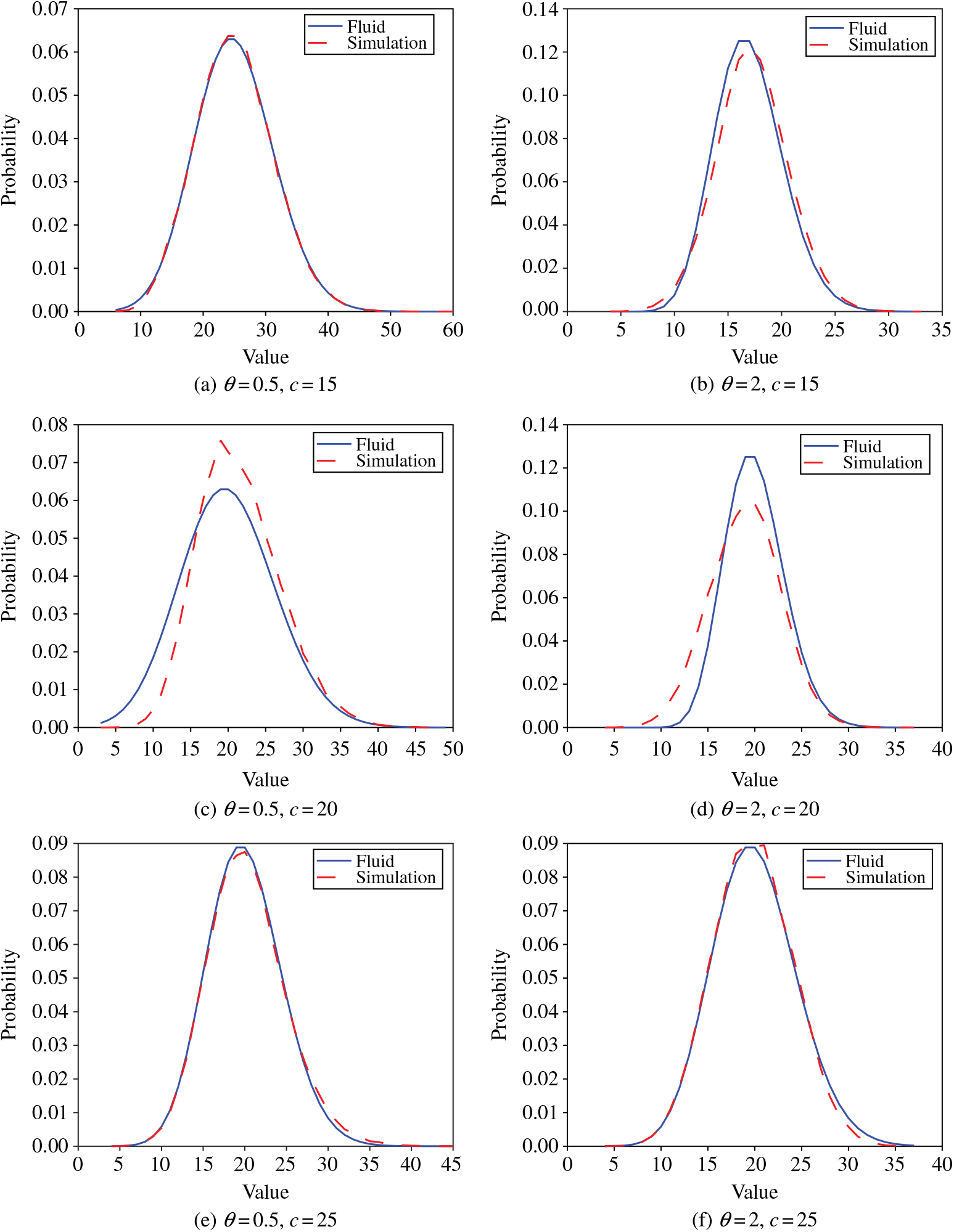
Figure 10. Empirical and fluid limiting distributions for λ = 20 and μ = 1.
In Figure 11 we examine the limiting distributions for the single server case. In these plots we set μ = 1 and then vary the arrival rate and the abandonment rate. For all plots on the left, we set θ = 0.5 and on the right θ = 2. Furthermore, for the top, middle, and bottom pairs of plots, we set λ to 0.8, 1, and 1.2, respectively. As in Figure 10, Figure 11 shows that our approximations are quite good. Thus, we are able to capture single server dynamics as well as large-scale multiserver dynamics even though they are quite different. This is even more useful as our approximations are nonasymptotic and do not rely on scaling the number of servers.
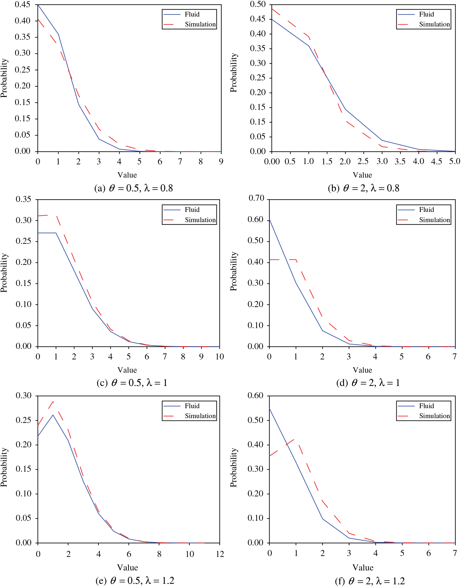
Figure 11. Empirical and fluid limiting distributions for c = 1 and μ = 1.
In Figure 12 we take the arrival rate as λ(t) = 6.5 + sin(t), the service rate as μ = 1, and the number of servers as c = 5. Because inft≥0λ(t) > cμ, we use the characterization of the fluid approximation as a shifted M/M/∞ queue and compare the simulated system, the fluid approximation, and the unshifted M/M/∞, as stated in Theorem 7. We consider the mean for θ = 1.1 and θ = 0.9 and find that while the fluid approximation is quite close the unshifted system is not near to the Erlang-A system, even for these relatively similar rates of service and abandonment. We note that the simulated values in Figure 12 are plotted using a dashed line, and the differences between these points and the fluid approximations can be most readily observed at the extremes of the trigonometric function.
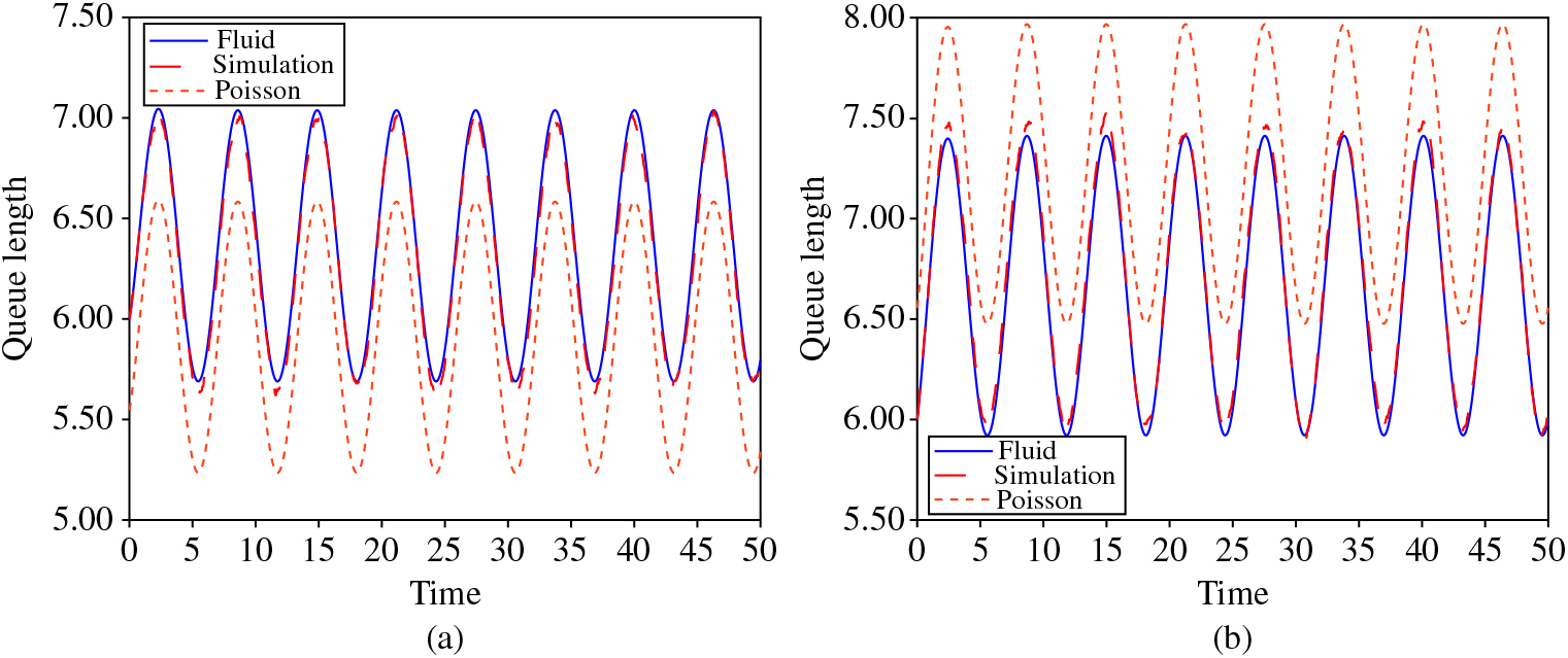
Figure 12. The queue mean for λ(t) = 6.5 + sin (t), μ = 1, Q(0) = 6, c = 5, and (a) θ = 1.1 and (b) θ = 0.9.
As a final comparison, in Table 1 we test the bounds in Theorems 4 and 5 by comparison to simulations of the first three moments. We perform this experiment with c = 10 and μ = 1 while taking λ ∈ {8, 10, 12} and θ ∈ {0.5, 2} so that we have considered all different conditions contained in these two results. As can also be observed in Figure 12, the empirical values are much closer to the fluid approximation than they are to the opposite bounds from Theorems 4 and 5. This is to be expected since the fluid values are the only intended approximation. Still, the pursuit of closer bounds in conjunction with the fluid approximation may be a future direction of practical importance.

5. Conclusion
In this paper we investigated the Erlang-A queueing system through comparison to the fluid approximations of its moments, moment generating function, and cumulant moment generating function. Through recognizing the convexity in the differential equations describing these approximations, we found fundamental relationships between the values of these quantities and their fluid counterparts: when the rate of abandonment is less than the rate of service the true value dominates the approximation, when the service rate is smaller the approximation dominates the true value, and when the rates of abandonment and service are equal, the two are equivalent. That is, for any (possibly nonstationary) arrival rate, and for θ as the abandonment rate and μ as the service rate, we can summarize these relationships as follows.
Note that the parameter conditions in Table 2 have actually been subjected to some specification in the case of the generating functions. As used in Subsections 4.1 and 4.2, the general conditions are actually (θ − μ)(e−α − 1)<0, (θ − μ)(e−α − 1) > 0, and (θ − μ)(e−α − 1) > 0. However, as we remarked previously, these conditions are equivalent when the space parameter of the generating functions is restricted to positive values, i.e. α > 0.
Table 2. Approximation characterization overview.
In forming these inequalities we have found explicit representations of the fluid approximations through equivalences in distribution with Poisson random variables and infinite-server queues, in cases of stationary and nonstationary arrival rates, respectively. The respective subsection references for these are Subsections 4.3 and 4.4. For convenience, in Table 3 we give an overview of the bounds and characterizations shown in this paper.
Table 3. Approximation characterization overview.
We note here that we use the notation M t/M(θ)/∞to represent an infinite-server queue with arrivals according to the nonstationary Poisson process with rate λ(t) as given in (12) and exponential service with rate θ > 0. We should also note that the periodic case also requires the initial number in system to be greater than c. These characterizations both give insight into the approximations themselves and yield natural inequalities that complement those from the approximations. We have demonstrated the performance of these bounds through simulations. Through consideration of both these findings and the empirical experiments, we can identify interesting directions for future work. For example, it would be of great interest to gain more explicit insights into the gap between the fluid approximations and the true values. This is a nontrivial endeavor, which stems from the nondifferentiability and nonclosure in the differential equations for the true expectations. The numerical experiments in this work indicate that the fluid approximations may often be quite close but not exact, and additional understanding would be useful in practice. Moreover, extending our results to more complicated queueing systems where the arrival and service processes follow phase type distributions is of interest given the new work of Ko and Pender [Reference Pender and Ko36], [Reference Ko and Pender22], [Reference Ko and Pender21].
It would be additionally useful to gain a better understanding of the limiting distribution of the Erlang-A queue. As we discuss in the paper, the empirical experiments in Subsection 4.5 indicate that the true limiting distributions closely resemble the shifted Poisson approximations. In particular, the approximations seem quite close when λ is not near cμ. As a simple extension of this work, it can be observed that some sort of combination of the approximation when λ < cμ and of the approximation when λ > cμ could make a nice choice for approximation of the distribution when λ = cμ. In some sense, it is not surprising that these approximations are similar to the true limiting distribution, as the Erlang-A queue appears to be an M/M/∞ queue with service rate μ (the approximation when λ < cμ), when only considering the states up to c, and it also resembles some sort of shifted M/M/∞ queue with service rate θ (which also describes the approximation when λ ≥ cμ) for states c + 1 and beyond.
Because the relationships between the true quantities and their approximations are conditioned only on the service and abandonment rate, it may be possible for this to be extended to stochastic-intensity, non-Poisson arrival processes, such as the Hawkes process or shot noise driven queues studied in [Reference Koops, Boxma and Mandjes23], [Reference Koops, Saxena, Boxma and Mandjes24], and [Reference Daw and Pender6]. Finally, in a similar manner it would be interesting to extend this to networks of Erlang-A queues; however, we would have to keep track of the routeing probabilities carefully to keep track of the convexity/concavity of the rate functions. We plan to consider these extensions in future work.
Acknowledgements
The authors are grateful for the generous support of the National Science Foundation through J. Pender’s Civil, Mechanical and Manufacturing Innovation (CMMI) Career Award (1751975), and A. Daw’s Graduate Research Fellowship (grant number DGE-1650441).


