


Introduction
All human communication requires common understandings of meaning. This is nowhere more true than political and social life, where the success of an appeal—rhetorical or otherwise—relies on an audience perceiving a message in the particular way that the speaker seeks to deliver it. Scholars have therefore spent much effort exploring the meanings of terms, how those meanings are manipulated, and how they change over time and space. Historically, this work has been qualitative (e.g., Austin Reference Austin1962; Geertz Reference Geertz1973; Skinner Reference Skinner1969). But in recent times, quantitative analysts have turned to modeling and measuring “context” directly from natural language (e.g., Aslett et al. Reference Aslett, Williams, Casas, Zuidema and Wilkerson2022; Hopkins Reference Hopkins2018; Park, Greene, and Colaresi Reference Park, Greene and Colaresi2020).
A promising avenue for such investigations has been the use of “word embeddings”—a family of techniques that conceive of meaning as emerging from the distribution of words that surround a term in text (e.g., Mikolov et al. Reference Mikolov, Sutskever, Chen, Corrado, Dean, Burges, Bottou, Welling, Ghahramani and Weinberger2013). By representing each word as a vector of real numbers and examining the relationships between vectors for the vocabulary of a corpus, scholars have uncovered new facts about language and the people that produce it (e.g., Caliskan, Bryson, and Narayanan Reference Caliskan, Bryson and Narayanan2017). This is also true in the study of politics, society, and culture (Garg et al. Reference Garg, Schiebinger, Jurafsky and Zou2018; Kozlowski, Taddy, and Evans Reference Kozlowski, Taddy and Evans2019; Rheault and Cochrane Reference Rheault and Cochrane2020; Rodman Reference Rodman2020; Wu et al. Reference Wu, Mebane, Woods, Klaver and Due2019).
Although borrowing existing techniques has certainly produced insights, for social scientists two problems remain. First, traditional approaches generally require a lot of data to produce high-quality representations—that is, to produce embeddings that make sense and connote meaning of terms correctly. The issue is less that our typical corpora are small—though they are compared with those on the web-scale collections often used in computer science—and more that terms for which we would like to estimate contexts are subject-specific and thus typically quite rare. As an example, there are fewer than twenty parliamentary mentions of the “special relationship” between the United States and the United Kingdom in some years of the 1980s—despite this arguably being the high watermark of elite closeness between the two countries. The second problem is one of inference. Although representations themselves are helpful, social scientists want to make statements about the statistical properties and relationships between embeddings. That is, they want to speak meaningfully of whether language is used differently across subcorpora and whether those apparent differences are larger than we would expect by chance. Neither of these problems are well addressed by current techniques. Although there have been efforts to address inference in embeddings (see, e.g, Kulkarni et al. Reference Kulkarni, Al-Rfou, Perozzi, Skiena, Gangemi, Leonardi and Panconesi2015; Lauretig Reference Lauretig, Volkov, Jurgens, Hovy, Bamman and Tsur2019), they are typically data intensive and computationally intensive.
We tackle these two problems together in what follows. We provide both a statistical framework for making statements about covariate effects on embeddings and one that performs particularly well in cases of rare words or small corpora. Specifically, we innovate on Khodak et al. (Reference Khodak, Saunshi, Liang, Ma, Stewart, Arora, Gurevych and Miya2018), which introduced à la carte embeddings (ALC). In a nutshell, the method takes embeddings that have been pretrained on large corpora (e.g., word2vec or GloVe embeddings readily available online), combined with a small sample of example uses for a focal word, and then induces a new context-specific embedding for the focal word. This requires only a simple linear transformation of the averaged embeddings for words within the context of the focal word.
We place ALC in a regression setting that allows for fast solutions to queries like “do authors with these covariate values use these terms in a different way than authors with different covariate values? If yes, how do they differ?” We provide three proofs of concept. First, we demonstrate the strength of our approach by comparing its performance to the “industry standard” as laid out by Rodman (Reference Rodman2020) in a study of a New York Times API corpus, where slow changes over long periods are the norm. Second, we show that our approach can estimate an approximate embedding even with only a single context. In particular, we demonstrate that we can separate individual instances of Trump and trump. Third, we show that our method can also identify drastic switches in meaning over short periods—specifically in our case, for the term Trump before and after the 2016 election.
We study three substantive cases to show how the technique may be put to work. First, we explore partisan differences in Congressional speech—a topic of long-standing interest in political science (see, e.g., Monroe, Colaresi, and Quinn Reference Monroe, Colaresi and Quinn2008). We show that immigration is, perhaps unsurprisingly, one of the most differently expressed terms for contemporary Democrats and Republicans. Our second substantive case is historical: we compare across polities (and corpora) to show how elites in the UK and US expressed empire in the postwar period, how that usage diverged, and when. Our third case shows how our approach can be used to measure sentiment. We build on earlier work (e.g., Osnabrügge, Hobolt, and Rodon Reference Osnabrügge, Hobolt and Rodon2021; Slapin et al. Reference Slapin, Kirkland, Lazzaro, Leslie and O’Grady2018) for the UK House of Commons, yielding novel insights about the relationship between the UK Prime Minister and his backbenchers on the European Union. We also provide advice to practitioners on how to use the technique based on extensive experiments reported in the Supplementary Materials (SM).
These innovations allow for social scientists to go beyond general meanings of words to capture situation-specific usage. This is possible without substantial computation and, in contrast to other approaches, requires only the text immediately around the word of interest.
We proceed as follows: in the next section, we provide some context for what social scientists mean by “context” and link this to the distribution of words around a focal term. We then introduce the ALC algorithm and provide three proofs of concept. Subsequently, we extend ALC to a regression framework and then present results from three substantive use cases. We give practical guidance on use and limitations before concluding.
Context in Context
… they are casting their problems on society and who is society? There is no such thing!
—Margaret Thatcher, interview with Woman’s Own (1987).Paraphrased as “there is no such thing as society,” Thatcher’s quote has produced lively debate in the study and practice of UK politics. Critics—especially from the left—argued that this was primarily an endorsement of individual selfishness and greed. But more sympathetic accounts have argued that the quote must be seen in its full context to be understood. The implication is that reading the line in its original surroundings changes the meaning: rather than embracing egotism, it emphasizes the importance of citizens’ obligations to each other above and beyond what the state requires.
Beyond this specific example, the measurement and modeling of context is obviously a general problem. In a basic sense, context is vital: we literally cannot understand what is meant by a speaker or author without it. This is partly due to polysemy—the word “society” might mean many different things. But the issue is broader than this and is at the core of human communication. Unsurprisingly then, the study of context has been a long-standing endeavor in social science. Its centrality has been emphasized in the history of ideas (Skinner Reference Skinner1969) through the lens of “speech acts” (Austin Reference Austin1962), describing cultural practices via “thick description” (Geertz Reference Geertz1973), understanding “political culture” (Verba and Almond Reference Verba and Almond1963), and the psychology of decision making (Tversky and Kahneman Reference Tversky and Kahneman1981).
Approaches to Studying Context
For the goal of describing context in observational data, social science has turned to text approaches—with topic models being popular (see Grimmer Reference Grimmer2010; Quinn et al. Reference Quinn, Monroe, Colaresi, Crespin and Radev2010; Roberts, Stewart, and Airoldi Reference Roberts, Stewart and Airoldi2016). Topic models provide a way to understand the allocation of attention across groupings of words.
Although such models have a built-in notion of polysemy (a single word can be allocated to different topics), they are rarely used as a mechanism for studying how individual words are used to convey different ideas (Grimmer and Stewart Reference Grimmer and Stewart2013). And though topic approaches do exist that allow for systematic variation in the use of a word across topics by different pieces of observed metadata (Roberts, Stewart, and Airoldi Reference Roberts, Stewart and Airoldi2016), they are computationally intensive (especially relative to the approaches we present below). The common unit of analysis for topic models is the document. This has implications for the way that these models capture the logic of the “distributional hypothesis”—the idea that, in the sense of Firth (Reference Firth1957, 11), “You shall know a word by the company it keeps”—in other words, that one can understand a particular version of the “meaning” of a term from the way it co-occurs with other terms. Specifically, in the case of topic models, the entire document is the context. From this we learn the relationships (the themes) between words and the documents in which they appear.
But in the questions we discuss here, the interest is in the contextual use of a specific word. To study this, social scientists have turned to word embeddings (e.g., Rheault and Cochrane Reference Rheault and Cochrane2020; Rodman Reference Rodman2020). For example, Caliskan, Bryson, and Narayanan (Reference Caliskan, Bryson and Narayanan2017) and Garg et al. (Reference Garg, Schiebinger, Jurafsky and Zou2018) have explored relationships between words captured by embeddings to describe problematic gender and ethnic stereotypes in society at large. Word embeddings predict a focal word as a function of the other words that appear within a small window of that focal word in the corpus (or the reverse, predict the neighboring words from the focal word). In so doing, they capture the insight of the distributional hypothesis in a very literal way: the context of a term are the tokens that appear near it in text, on average. In practice, this is all operationalized via a matrix of co-occurrences of words that respect the relevant window size. In the limit, where we imagine the relevant window is the entire document, one can produce a topic model from the co-occurrence matrix directly. Thus as the context window in the embedding model approaches the length of the document, the embeddings will increasingly look like the word representations in a topic model.
Whether, and in what way, embedding models based on the distributional hypothesis capture “meaning” is more controversial. Here we take a narrow, “structuralist” (in the sense of Harris Reference Harris1954) view. For this paper, meaning is in terms of description and is empirical. That is, it arises from word co-occurrences in the data, alone: we will neither construct nor assume a given theoretical model of language or cognition. And, in contrast to other scholars (e.g., Miller and Charles Reference Miller and Charles1991), we will make no claims that the distributions per se have causal effects on human understandings of terms. Thus, when we speak of the meaning of a focal word being different across groups, we are talking in a thin sense about the distribution of other words within a fixed window size of that focal word being different. Though we will offer guidance, substantive interpretation of these differences for a given purpose is ultimately up to the researcher. That is, as always with such text measurement strategies, subject-expert validation is important.
For a variety of use cases, social scientists want to make systematic inferences about embeddings—which requires statements about uncertainty. Suppose we wish to compare the context of “society” as conveyed by British Prime Ministers with that of US Presidents. Do they differ in a statistically significant way? To judge this, we need some notion of a null hypothesis, some understanding of the variance of our estimates, and a test statistic. Although there have been efforts to compare embeddings across groups (Rudolph et al. Reference Rudolph, Ruiz, Athey, Blei, Guyon, Von Luxburg, Bengio, Wallach, Fergus, Vishwanathan and Garnett2017) and to give frameworks for such conditional relationships (Han et al. Reference Han, Gill, Spirling, Cho, Riloff, Chiang, Hockenmaier and Tsujii2018), these are nontrivial to implement. Perhaps more problematically for most social science cases is that they rely on underlying embedding models that struggle to produce “good” representations—that make sense and correctly capture how that word is actually used—when we have few instances of a term of interest. This matters because we are typically far short of the word numbers that standard models require for optimal performance and terms (like “society”) may be used in ways that are idiosyncratic to a particular document or author.
In the next section, we will explain how we build on earlier insights from ALC embeddings (Khodak et al. Reference Khodak, Saunshi, Liang, Ma, Stewart, Arora, Gurevych and Miya2018) to solve these problems in a fast, simple, and sample-efficient “regression” framework. Before doing so, we note three substantive use cases that both motivate the methodological work we do and show its power as a tool for social scientists. The exercise in all cases is linguistic discovery insofar as our priors are not especially sharp and the primary value is in stimulating more productive engagement with the text. Nonetheless, in using the specific approach we outline in this paper, we will be able to make inferences with attendant statements about uncertainty. In that sense, our examples are intended to be illuminating for other scholars comparing corpora or comparing authors within a corpus.
Use Case I: Partisan Differences in Word Usage
A common problem in Americanist political science is to estimate partisan differences in the usage of a given term. Put literally, do Republicans and Democrats mean something different when they use otherwise identical words like immigration and marriage? Although there have been efforts to understand differential word rate of use within topics pertaining to these terms (e.g., Monroe, Colaresi, and Quinn Reference Monroe, Colaresi and Quinn2008), there has been relatively little work on whether the same words appear in different contexts. Below, we use the Congressional Record (Sessions 111–114) as our corpus for this study (Gentzkow, Shapiro, and Taddy Reference Gentzkow, Shapiro and Taddy2018). This requires that we compare embeddings as a function of party (and other covariates).
Use Case II: Changing UK–US Understandings of “Empire”
The United Kingdom’s relative decline as a Great Power during the postwar period has been well documented (e.g., Hennessy Reference Hennessy1992). One way that we might investigate the timing of US dominance (over the UK, at least) is to study the changing understanding of the term Empire in both places. That is, beyond any attitudinal shift, did American and British policy makers alter the way they used empire as the century wore on? If they did, when did this occur? And did the elites of these countries converge or diverge in terms of their associations of the term? To answer these questions, we will statistically compare the embedding for the term Empire for the UK House of Commons (via Hansard) versus the US Congress (via the Congressional Record) from 1935–2010.
Use Case III: Brexit Sentiment from the Backbenches
The UK’s decision to leave the European Union (EU) following the 2016 referendum was momentous (Ford and Goodwin Reference Ford and Goodwin2017). Although the vote itself was up to citizens, the build-up to the plebiscite was a matter for elites; specifically, it was a consequence of the internal machinations of the parliamentary Conservative Party that forced the hand of their leader, Prime Minster David Cameron (Hobolt Reference Hobolt2016). A natural question concerns the attitudes of that party in the House of Commons toward the EU, both over time and relative to other issue areas (such as education and health policy). To assess that, we will use an embedding approach to sentiment estimation for single instances of terms that builds on recent work on emotion in parliament (Osnabrügge, Hobolt, and Rodon Reference Osnabrügge, Hobolt and Rodon2021). This will also allow us to contribute to the literature on Member of Parliament (MP) position taking via speech (see, e.g., Slapin et al. Reference Slapin, Kirkland, Lazzaro, Leslie and O’Grady2018).
Using ALC Embeddings to Measure Meaning
Our methodological goal is a regression framework for embeddings. By “regression” we mean two related ideas. Narrowly, we mean that we want to be able to approximate a conditional expectation function, typically written $ \unicode{x1D53C}\left[Y|X\right] $
where, as usual,
$ \unicode{x1D53C}\left[Y|X\right] $
where, as usual, $ Y $
is our outcome,
$ Y $
is our outcome, $ X $
is a particular covariate, and
$ X $
is a particular covariate, and $ \unicode{x1D53C} $
is the expectations operator. We want to make statements about how embeddings (our Y) differ as covariates (our X) change. More broadly, we use “regression” to mean machinery for testing hypotheses about whether the groups actually differ in a systematic way. And by extension, we want that machinery to provide tools for making downstream comments about how those embeddings differ. In all cases, this will require three related operations:
$ \unicode{x1D53C} $
is the expectations operator. We want to make statements about how embeddings (our Y) differ as covariates (our X) change. More broadly, we use “regression” to mean machinery for testing hypotheses about whether the groups actually differ in a systematic way. And by extension, we want that machinery to provide tools for making downstream comments about how those embeddings differ. In all cases, this will require three related operations:
-
1. an efficient and transparent way to embed words such that we can produce high-quality representations even when a given word is rare;
-
2. given (1), a demonstration that in real problems, a single instance of a word’s use is enough to produce a good embedding. This allows us to set up the hypothesis-testing problem as a multivariate regression and is the subject of the next section;
-
3. given (1) and (2), a method for making claims about the statistical significance of differences in embeddings, based on covariate profiles. We tackle that below.
Ideally, our framework will deliver good representations of meaning even in cases where we have very few incidences of the words in question. À la carte embeddings (Khodak et al. Reference Khodak, Saunshi, Liang, Ma, Stewart, Arora, Gurevych and Miya2018) promise exactly this. We now give some background and intuition on that technique. We then replicate Rodman (Reference Rodman2020)—a recent study introducing time-dependent word embeddings for political science—to demonstrate ALC’s efficiency and quality.
Word Embeddings Measure Meaning through Word Co-Occurence
Word embeddings techniques give every word a distributed representation—that is, a vector. The length or dimension (D) of this vector is—by convention—between 100 and 500. When the inner product between two different words (two different vectors) is high, we infer that they are likely to co-occur in similar contexts. The distributional hypothesis then allows us to infer that those two words are similar in meaning. Although such techniques are not new conceptually (e.g., Hinton Reference Hinton1986), methodological advances in the last decade (Mikolov et al. Reference Mikolov, Sutskever, Chen, Corrado, Dean, Burges, Bottou, Welling, Ghahramani and Weinberger2013; Pennington, Socher, and Manning Reference Pennington, Socher, Manning, Specia and Carreras2014) allow them to be estimated much more quickly. More substantively, word embeddings have been shown to be useful, both as inputs to supervised learning problems and for understanding language directly. For example, embedding representations can be used to solve analogy reasoning tasks, implying the vectors do indeed capture relational meaning between words (e.g., Arora et al. Reference Arora, Li, Liang, Ma and Risteski2018; Mikolov et al. Reference Mikolov, Sutskever, Chen, Corrado, Dean, Burges, Bottou, Welling, Ghahramani and Weinberger2013).
Understanding exactly why word embeddings work is nontrivial. In any case, there is now a large literature proposing variants of the original techniques (e.g., Faruqui et al. Reference Faruqui, Dodge, Jauhar, Dyer, Hovy, Smith, Mihalcea, Chai and Sarkar2015; Lauretig Reference Lauretig, Volkov, Jurgens, Hovy, Bamman and Tsur2019). A few of these are geared specifically to social science applications where the general interest is in measuring changes in meanings, especially via “nearest neighbors” of specific words.
Although the learned embeddings provide a rough sense of what a word means, it is difficult to use them to answer questions of the sort we posed above. Consider our interest in how Republicans and Democrats use the same word (e.g., immigration) differently. If we train a set of word embeddings on the entire Congressional Record we only have a single meaning of the word. We could instead train a separate set of embeddings—one for Republicans and one for Democrats—and then realign them. This is an extra computational step and may not be feasible in other use cases where the vocabularies do not have much overlap. We now discuss a way to proceed that is considerably easier.
A Random Walk Theoretical Framework and ALC Embeddings
The core of our approach is ALC embeddings. The theory behind that approach is given by Arora et al. (Reference Arora, Li, Liang, Ma and Risteski2016) and Arora et al. (Reference Arora, Li, Liang, Ma and Risteski2018). Those papers conceive of documents being a “random walk” in a discourse space, where words are more likely to follow other words if they are closer to them in an embedding space. Crucially for ALC, Arora et al. (Reference Arora, Li, Liang, Ma and Risteski2018) also proves that under this model, a particular relationship will follow for the embedding of a word and the embeddings of the words that appear in the contexts around it.
To fix ideas, consider the following toy example. Our corpus is the memoirs of a politician, and we observe two entries, both mentioning the word “bill”:
-
1. The debate lasted hours, but finally we [voted on the
 and it passed] with a large majority.
 -
2. At the restaurant we ran up [a huge wine
to be paid] by our host.
As one can gather from the context—here, the three words either side of the instance of “bill” in square brackets—the politician is using the term in two different (but grammatically correct) ways.
The main result from Arora et al. (Reference Arora, Li, Liang, Ma and Risteski2018) shows the following: if the random walk model holds, the researcher can obtain an embedding for word $ w $
(e.g., “bill”) by taking the average of the embeddings of the words around
$ w $
(e.g., “bill”) by taking the average of the embeddings of the words around $ w $
(
$ w $
( $ {\mathbf{u}}_w) $
and multiplying them by a particular square matrix
$ {\mathbf{u}}_w) $
and multiplying them by a particular square matrix $ \mathbf{A} $
. That
$ \mathbf{A} $
. That $ \mathbf{A} $
serves to downweight the contributions of very common (but uninformative) words when averaging. Put otherwise, if we can take averages of some vectors of words that surround
$ \mathbf{A} $
serves to downweight the contributions of very common (but uninformative) words when averaging. Put otherwise, if we can take averages of some vectors of words that surround $ w $
(based on some preexisting set of embeddings
$ w $
(based on some preexisting set of embeddings $ {\mathbf{v}}_w $
) and if we can find a way to obtain
$ {\mathbf{v}}_w $
) and if we can find a way to obtain $ \mathbf{A} $
(which we will see is also straightforward), we can provide new embeddings for even very rare words. And we can do this almost instantaneously.
$ \mathbf{A} $
(which we will see is also straightforward), we can provide new embeddings for even very rare words. And we can do this almost instantaneously.
Returning to our toy example, consider the first, legislative, use of “bill” and the words around it. Suppose we have embedding vectors for those words from some other larger corpus, like Wikipedia. To keep things compact, we will suppose those embeddings are all of three dimensions (such that $ D=3 $
), and take the following values:
$ D=3 $
), and take the following values:
 $$ \underset{\mathrm{voted}}{\underbrace{\left[\begin{array}{c}-1.22\\ {}1.33\\ {}0.53\end{array}\right]}}\underset{\mathrm{on}}{\underbrace{\left[\begin{array}{c}1.83\\ {}0.56\\ {}-0.81\end{array}\right]}}\underset{\mathrm{the}}{\underbrace{\left[\begin{array}{c}-0.06\\ {}-0.73\\ {}0.82\end{array}\right]}}\hskip0.30em \mathrm{bill}\hskip0.1em \underset{\mathrm{and}}{\underbrace{\left[\begin{array}{c}1.81\\ {}1.86\\ {}1.57\end{array}\right]}}\underset{\mathrm{it}}{\underbrace{\left[\begin{array}{c}-1.50\\ {}-1.65\\ {}0.48\end{array}\right]}}\underset{\mathrm{passed}}{\underbrace{\left[\begin{array}{c}-0.12\\ {}1.63\\ {}-0.17\end{array}\right]}}. $$
Obtaining $ {\mathbf{u}}_w $
for “bill: simply requires averaging these vectors and thus
$ {\mathbf{u}}_w $
for “bill: simply requires averaging these vectors and thus
 $$ {\mathbf{u}}_{{\mathrm{bill}}_1}=\left[\begin{array}{c}0.12\\ {}0.50\\ {}0.40\end{array}\right], $$
with the subscript denoting the first use case. We can do the same for the second case—the restaurant sense of “bill”—from the vectors of a, huge, wine, to, be, and paid. We obtain
 $$ {\mathbf{u}}_{{\mathrm{bill}}_2}=\left[\begin{array}{c}0.35\\ {}-0.38\\ {}-0.24\end{array}\right], $$
which differs from the average for the first meaning. A reasonable instinct is that these two vectors should be enough to give us an embedding for “bill” in the two senses. Unfortunately, they will not—this is shown empirically in Khodak et al. (Reference Khodak, Saunshi, Liang, Ma, Stewart, Arora, Gurevych and Miya2018) and in our Trump/trump example below. As implied above, the intuition is that simply averaging embeddings overexaggerates common components associated with frequent (e.g., “stop”) words. So we will need the $ \mathbf{A} $
matrix too: it down-weights these directions so they don’t overwhelm the induced embedding.
$ \mathbf{A} $
matrix too: it down-weights these directions so they don’t overwhelm the induced embedding.
Khodak et al. (Reference Khodak, Saunshi, Liang, Ma, Stewart, Arora, Gurevych and Miya2018) show how to put this logic into practice. The idea is that a large corpus (generally the corpus the embeddings were originally trained on, such as Wikipedia) can be used to estimate the transformation matrix $ \mathbf{A} $
. This is a one time cost after which each new word embedding can be computed à la carte (thus the name), rather than needing to retrain an entire corpus just to get the embedding for a single word. As a practical matter, the estimator for
$ \mathbf{A} $
. This is a one time cost after which each new word embedding can be computed à la carte (thus the name), rather than needing to retrain an entire corpus just to get the embedding for a single word. As a practical matter, the estimator for $ \mathbf{A} $
can be learned efficiently with a lightly modified linear regression model that reweights the words by a nondecreasing function
$ \mathbf{A} $
can be learned efficiently with a lightly modified linear regression model that reweights the words by a nondecreasing function $ \alpha \left(\cdot \right) $
of the total instances of each word (
$ \alpha \left(\cdot \right) $
of the total instances of each word ( $ {n}_w $
) in the corpus. This reweighting addresses the fact that words that appear more frequently have embeddings that are measured with greater certainty. Thus we learn the transformation matrix as,
$ {n}_w $
) in the corpus. This reweighting addresses the fact that words that appear more frequently have embeddings that are measured with greater certainty. Thus we learn the transformation matrix as,
 $$ \hat{\mathbf{A}}=\underset{\mathbf{A}}{\mathrm{argmin}}{\sum}_{w=1}^W\alpha \left({n}_w\right)\parallel {\mathbf{v}}_w-\mathbf{A}{\mathbf{u}}_w{\parallel}_2^2. $$
The natural log is a simple choice for $ \alpha \left(\cdot \right) $
, and works well. Given
$ \alpha \left(\cdot \right) $
, and works well. Given $ \hat{\mathbf{A}} $
, we can introduce new embeddings for any word by averaging the existing embeddings for all words in its context to create
$ \hat{\mathbf{A}} $
, we can introduce new embeddings for any word by averaging the existing embeddings for all words in its context to create $ {\mathbf{u}}_{\mathrm{w}} $
and then applying the transformation such that
$ {\mathbf{u}}_{\mathrm{w}} $
and then applying the transformation such that $ {\hat{\mathbf{v}}}_w=\hat{\mathbf{A}}{\mathbf{u}}_w $
. The transformation matrix is not particularly hard to learn (it is a linear regression problem), and each subsequent induced word embedding is a single matrix multiply.
$ {\hat{\mathbf{v}}}_w=\hat{\mathbf{A}}{\mathbf{u}}_w $
. The transformation matrix is not particularly hard to learn (it is a linear regression problem), and each subsequent induced word embedding is a single matrix multiply.
Returning to our toy example, suppose that we estimate $ \hat{\mathbf{A}} $
from a large corpus like Hansard or the Congressional Record or wherever we obtained the embeddings for the words that surround “bill.” Suppose that we estimate
$ \hat{\mathbf{A}} $
from a large corpus like Hansard or the Congressional Record or wherever we obtained the embeddings for the words that surround “bill.” Suppose that we estimate
 $$ \hat{\mathbf{A}}=\left[\begin{array}{ccc}0.81& 3.96& 2.86\\ {}2.02& 4.81& 1.93\\ {}3.14& 3.81& 1.13\end{array}\right]. $$
Taking inner products, we have
 $$ {\hat{\mathbf{v}}}_{{\mathrm{bill}}_1}=\hat{\mathbf{A}}\cdot {\mathbf{u}}_{{\mathrm{bill}}_1}=\hskip-0.2em \left[\begin{array}{c}3.22\\ {}3.42\\ {}2.73\end{array}\right]\hskip0.20em \mathrm{and}\hskip0.5em {\hat{\mathbf{v}}}_{{\mathrm{bill}}_2}\hskip-0.2em =\hat{\mathbf{A}}\cdot {\mathbf{u}}_{{\mathrm{bill}}_2}=\left[\begin{array}{c}-1.91\\ {}-1.58\\ {}-0.62\end{array}\right]. $$
These two transformed embeddings vectors are more different than they were—a result of down-weighting the commonly appearing words around them—but that is not the point per se. Rather, we expect them to be informative about the word sense by, for example, comparing them to other (preestimated) embeddings in terms of distance. Thus we might find that the nearest neighbors of $ {\hat{\mathbf{v}}}_{{\mathrm{bill}}_1} $
are
$ {\hat{\mathbf{v}}}_{{\mathrm{bill}}_1} $
are
 $$ \mathrm{legislation}=\left[\begin{array}{c}3.11\\ {}2.52\\ {}3.38\end{array}\right]\hskip1em \mathrm{and}\hskip1em \mathrm{amendment}=\left[\begin{array}{c}2.15\\ {}2.47\\ {}3.42\end{array}\right], $$
whereas the nearest neighbors of $ {\hat{\mathbf{v}}}_{{\mathrm{bill}}_2} $
are
$ {\hat{\mathbf{v}}}_{{\mathrm{bill}}_2} $
are
 $$ \mathrm{dollars}=\left[\begin{array}{c}-1.92\\ {}-1.54\\ {}-0.60\end{array}\right]\hskip1em \mathrm{and}\hskip1em \mathrm{cost}=\left[\begin{array}{c}-1.95\\ {}-1.61\\ {}-0.63\end{array}\right]. $$
This makes sense, given how we would typically read the politician’s lines above. The key here is that the ALC method allowed us to infer the meaning of words that occurred rarely in a small corpus (the memoirs) without having to build embeddings for those rare words in that small corpus: we could “borrow’” and transform the embeddings from another source. Well beyond this toy example, Khodak et al. (Reference Khodak, Saunshi, Liang, Ma, Stewart, Arora, Gurevych and Miya2018) finds empirically that the learned $ \hat{\mathbf{A}} $
in a large corpus recovers the original word vectors with high accuracy (greater than 0.90 cosine similarity). They also demonstrate that this strategy achieves state-of-the-art and near state-of-the-art performance on a wide variety of natural language processing tasks (e.g., learning the embedding of a word using only its definition, learning meaningful n-grams, classification tasks, etc.) at a fraction of the computational cost of the alternatives.
$ \hat{\mathbf{A}} $
in a large corpus recovers the original word vectors with high accuracy (greater than 0.90 cosine similarity). They also demonstrate that this strategy achieves state-of-the-art and near state-of-the-art performance on a wide variety of natural language processing tasks (e.g., learning the embedding of a word using only its definition, learning meaningful n-grams, classification tasks, etc.) at a fraction of the computational cost of the alternatives.
The ALC framework has three major advantages for our setting: transparency, computational ease, and efficiency. First, compared with many other embedding strategies for calculating conditional embeddings (e.g., words over time) the information used in ALC is transparent. The embeddings are derived directly from the additive information of the words in the context window around the focal word; there is no additional smoothing or complex interactions across different words. Furthermore, the embedding space itself does not change, it remains fixed to the space defined by the pretrained embeddings. Second, this same transparency leads to computational ease. The transformation matrix $ \mathbf{A} $
only has to be estimated once, and then each subsequent induction of a new word is a single matrix multiply and thus effectively instantaneous. Later we will be able to exploit this speed to allow bootstrapping and permutation procedures that would be unthinkable if there was an expensive model fitting procedure for each word. Finally, ALC is efficient in the use of information. Once the transformation matrix is estimated, it is only necessary that
$ \mathbf{A} $
only has to be estimated once, and then each subsequent induction of a new word is a single matrix multiply and thus effectively instantaneous. Later we will be able to exploit this speed to allow bootstrapping and permutation procedures that would be unthinkable if there was an expensive model fitting procedure for each word. Finally, ALC is efficient in the use of information. Once the transformation matrix is estimated, it is only necessary that $ {\mathbf{u}}_w $
converges—in other words, we only need to estimate a
$ {\mathbf{u}}_w $
converges—in other words, we only need to estimate a $ D $
-dimensional mean from a set of samples. In the case of a six-word symmetric context window, there are 12 words total within the context window; thus, for each instance of the focal word we have a sample of size 12 from which to estimate the mean.
$ D $
-dimensional mean from a set of samples. In the case of a six-word symmetric context window, there are 12 words total within the context window; thus, for each instance of the focal word we have a sample of size 12 from which to estimate the mean.
Although Khodak et al. (Reference Khodak, Saunshi, Liang, Ma, Stewart, Arora, Gurevych and Miya2018) focused on using the ALC framework to induce embeddings for rare words and phrases, we will apply this technique to embed words used in different partitions of a single corpus or to compare across corpora. This allows us to capture differences in embeddings over time or by speaker, even when we have only a few instances within each sample. Importantly, unlike other methods, we don’t need an entirely new corpus to learn embeddings for select focal words; we can select particular words and calculate (only) their embeddings using only the contexts around those particular words.Footnote 1 We now demonstrate this power of ALC by replicating Rodman (Reference Rodman2020).Footnote 2
Proof of Concept for ALC in Small Political Science Corpora: Reanalyzing Rodman (Reference Rodman2020)
The task in Rodman (Reference Rodman2020) is to understand changes in the meaning of equality over the period 1855–2016 in a corpus consisting of the headlines and other summaries of news articles.Footnote 3 As a gold standard, a subset of the articles is hand-coded into 15 topic word categories—of which five are ultimately used in the analysis—and the remaining articles are coded using a supervised topic model with the hand-coded data as input. Four embeddings techniques are used to approximate trends in coverage of those categories, via the (cosine) distance between the embedding for the word equality and the embeddings for the category labels. This is challenging because the corpus is small—the first 25-year slice of data has only 71 documents—and in almost 30% of the word-slice combinations there are fewer than 10 observations.Footnote 4
Rodman (Reference Rodman2020) tests four different methods by comparing results to the gold standard; ultimately, the chronologically trained model (Kim et al. Reference Kim, Chiu, Hanaki, Hegde, Petrov, Danescu-Niculescu-Mizil, Eisenstein, McKeown and Smith2014) is the best performer. In each era (of 25 years), the model is fit several times on a bootstrap resampled collection of documents and then averaged over the resulting solutions (Antoniak and Mimno Reference Antoniak and Mimno2018). Importantly, the model in period $ t $
is initialized with period t–1 embeddings, whereas the first period is initialized with vectors trained on the full corpus. Even for a relatively small corpus, this process is computationally expensive, and our replication took about five hours of compute time on an eight-core machine.
$ t $
is initialized with period t–1 embeddings, whereas the first period is initialized with vectors trained on the full corpus. Even for a relatively small corpus, this process is computationally expensive, and our replication took about five hours of compute time on an eight-core machine.
The ALC approach to the problem is simple. For each period we use ALC to induce a period-specific embedding for equality as well as each of the five category words: gender, treaty, german, race, and african_american. We use GloVe pretrained embeddings and the corresponding transformation matrix estimated by Khodak et al. (Reference Khodak, Saunshi, Liang, Ma, Stewart, Arora, Gurevych and Miya2018)—in other words, we make use of no corpus-specific information in the initial embeddings and require as inputs only the context window around each category word. Following Rodman, we compute the cosine similarity between equality and each of the five category words, for each period. We then standardize (make into $ z $
-scores) those similarities. The entire process is transparent and takes only a few milliseconds (the embeddings themselves involve six matrix multiplies).
$ z $
-scores) those similarities. The entire process is transparent and takes only a few milliseconds (the embeddings themselves involve six matrix multiplies).
How does ALC do? Figure 1 is the equivalent of Figure 3 in Rodman (Reference Rodman2020). It displays the normalized cosine similarities for the chronological model (CHR, taken from Rodman Reference Rodman2020) and ALC, along with the gold standard (GS). We observe that ALC tracks approximately as well as does Rodman’s chronological model on its own terms. Where ALC clearly does better is on each model’s nearest neighbors (Tables 1 and 2): it produces more semantically interpretable and conceptually precise nearest neighbors than the chronological model.

Figure 1. Replication of Figure 3 in Rodman (Reference Rodman2020) Adding ALC Results
Note: ALC = ALC model, CHR = chronological model, and GS = gold standard.
Table 1. Nearest Neighbors for the 1855 Corpus

Table 2. Nearest Neighbors for the 2005 Corpus

We emphasize that in the 1855 corpus, four of the five category words (all except african_american) are estimated using five or fewer instances. Whereas the chronological model is sharing information across periods, ALC is treating each slice separately, meaning that our analysis could be conducted effectively with even fewer periods.
Collectively, these results suggest that ALC is competitive with the current state of the art within the kind of small corpora that arise in social science settings. We now turn to providing a hypothesis-testing framework that will allow us to answer the types of questions we introduced above.
Testing Hypotheses about Embeddings
Ultimately we want to speak of the way that embeddings differ systematically across levels of covariates. To do this, we will set up a regression-like framework, where each “observation” is the embedding of a single word. À la carte embeddings will assist us, but first we show that it can learn meaningful embeddings from one example use.
À la Carte on Text Can Distinguish Word Meanings from One Example Use
Above we explained that ALC averaged pretrained embeddings and then applied a linear transformation. This new embedding vector has, say, 300 dimensions, and we might reasonably be concerned that it is too noisy to be useful. To evaluate this, we need a ground truth. So we study a recent New York Times corpus; based on lead paragraphs, we show that we can reliably distinguish Trump the person (2017–2020) from other sense of trump as a verb or noun (1990–2020).Footnote 5
For each sense of the word (based on capitalization), we take a random sample with replacement of 400 realizations—the number of instances of trump in our corpus—from our New York Times corpus and embed them using ALC. We apply $ k $
-means clustering with two clusters to the set of embedded instances and evaluate whether the clusters partition the two senses. If ALC works, we should obtain two separate clouds of points that are internally consistent (in terms of the word sense). This is approximately what we see. Figure 2 provides a visualization of the 300-dimensional space projected to two dimensions with Principal Components Analysis (PCA) and identifying the two clusters by their dominant word sense. We explicitly mark misclassifications with an
$ k $
-means clustering with two clusters to the set of embedded instances and evaluate whether the clusters partition the two senses. If ALC works, we should obtain two separate clouds of points that are internally consistent (in terms of the word sense). This is approximately what we see. Figure 2 provides a visualization of the 300-dimensional space projected to two dimensions with Principal Components Analysis (PCA) and identifying the two clusters by their dominant word sense. We explicitly mark misclassifications with an $ x $
.
$ x $
.

Figure 2. Identification of Distinct Clusters
Note: Each observation represents a single realization of a target word, either of trump or Trump. Misclassified instances refer to instances of either target word that were assigned the majority cluster of the opposite target word.
To provide a quantitative measure of performance we compute the average cluster homogeneity: the degree to which each cluster contains only members of a given class. This value ranges between 0—both clusters have equal numbers of both context types—and 1—each cluster consists entirely of a single context type. By way of comparison, we do the same exercise using other popular methods of computing word vectors for each target realization including latent semantic analysis (LSA), simple averaging of the corresponding pretrained embeddings (ALC without transformation by $ \mathbf{A}), $
and RoBERTa contextual embeddings (Liu et al. Reference Liu, Ott, Goyal, Du, Joshi, Chen, Levy, Lewis, Zettlemoyer and Stoyanov2019).Footnote 6, Footnote 7 To quantify uncertainty in our metric, we use block bootstrapping—resampling individual instances of the focal word.Footnote 8 Figure 3 summarizes our results.
$ \mathbf{A}), $
and RoBERTa contextual embeddings (Liu et al. Reference Liu, Ott, Goyal, Du, Joshi, Chen, Levy, Lewis, Zettlemoyer and Stoyanov2019).Footnote 6, Footnote 7 To quantify uncertainty in our metric, we use block bootstrapping—resampling individual instances of the focal word.Footnote 8 Figure 3 summarizes our results.

Figure 3. Cluster Homogeneity
Note: Cluster homogeneity (in terms of Trump vs. trump) of k-means with two clusters of individual term instances embedded using different methods.
Latent sematic analysis does not fare well in this task; ALC, on the other hand, performs close to on par with transformer-based RoBERTa embeddings.Footnote 9 Simple averaging of embeddings also performs surprisingly well, coming out on top in this comparison. Does this mean the linear transformation that distinguishes ALC from simple averaging is redundant? To evaluate this, we look at nearest neighbors using both methods. Table 3 displays these results. We observe that simple averaging of embeddings produces mainly stopwords as nearest neighbors. The ALC method, on the other hand, outputs nearest neighbors aligned with the meaning of each term, Trump is associated with president Trump, whereas trump is largely associated with its two related other meanings: a suit in trick-taking games and defeating someone. This serves to highlight the importance of the linear transformation $ \mathbf{A} $
in the ALC method.
$ \mathbf{A} $
in the ALC method.
Table 3. Top 10 Nearest Neighbors Using Simple Averaging of Embeddings and ALC

Although this example is a relatively straightforward case of polysemy, we also know that the meaning of Trump, the surname, underwent a significant transformation once Donald J. Trump was elected president of the United States in November 2016. This is a substantially harder case because the person being referred to is still the same, even though the contexts it is employed in—and thus in the sense of the distributional hypothesis, the meaning—has shifted. But as we show in Supplementary Materials B, ALC has no problem with this case either, returning excellent cluster homogeneity and nearest neighbors.
The good news for the Trump examples is that ALC can produce reasonable embeddings even from single instances. Next we demonstrate that each of these instances can be treated as an observation in a hypothesis-testing framework. Before doing so, although readers may be satisfied about the performance of ALC in small samples, they may wonder about its performance in large samples. That is, whether it converges to the inferences one would make from a “full” corpus model as the number of instances increases; the answer is “yes,” and we provide more details in Supplementary Materials C.
À la Carte on Text Embedding Regression Model: conText
Recall the original statement of the relationship between the embedding of a focal word and the embeddings of the words within its context: $ {\mathbf{v}}_w=\mathbf{A}{\mathbf{u}}_w={\mathbf{A}\unicode{x1D53C}}_c[{\mathbf{u}}_{wc}] $
, where the expectation is taken over the contexts, c. Here we note that because the matrix
$ {\mathbf{v}}_w=\mathbf{A}{\mathbf{u}}_w={\mathbf{A}\unicode{x1D53C}}_c[{\mathbf{u}}_{wc}] $
, where the expectation is taken over the contexts, c. Here we note that because the matrix $ \mathbf{A} $
is constant we can easily swap it into the expectation and then calculate the resulting expectation conditional on some covariate
$ \mathbf{A} $
is constant we can easily swap it into the expectation and then calculate the resulting expectation conditional on some covariate $ X $
:
$ X $
: $ \unicode{x1D53C}\left[\mathbf{A}{\mathbf{u}}_w|X\right] $
. In particular, this can be done implicitly through a multivariate regression procedure. In the case of word meanings in discrete subgroups, this is exactly the same as the use of ALC applied above.
$ \unicode{x1D53C}\left[\mathbf{A}{\mathbf{u}}_w|X\right] $
. In particular, this can be done implicitly through a multivariate regression procedure. In the case of word meanings in discrete subgroups, this is exactly the same as the use of ALC applied above.
To illustrate our set up, suppose that each $ {\mathbf{v}}_{w_i} $
is the embedding of a particular instance of a given word in some particular context, like Trump. Each is of some dimension,
$ {\mathbf{v}}_{w_i} $
is the embedding of a particular instance of a given word in some particular context, like Trump. Each is of some dimension, $ D $
and thus each observation in this setting is a
$ D $
and thus each observation in this setting is a $ 1\times D $
embedding vector. We can stack these to produce an outcome variable
$ 1\times D $
embedding vector. We can stack these to produce an outcome variable $ \mathbf{Y} $
, which is of dimensions
$ \mathbf{Y} $
, which is of dimensions $ n $
(the number of instances of a given word) by D. The usual multivariate matrix equation is then
$ n $
(the number of instances of a given word) by D. The usual multivariate matrix equation is then
 $$ \underset{n\times D}{\underbrace{\mathbf{Y}}}=\underset{n\times p+1}{\underbrace{\mathbf{X}}}\underset{p+1\times D}{\underbrace{\beta}}+\underset{n\times D}{\underbrace{\mathbf{E}}}, $$
where $ \mathbf{X} $
is a matrix of p covariates and includes a constant term, whereas β is a set of p coefficients and an intercept (all of dimension D). Then E is an error term.
$ \mathbf{X} $
is a matrix of p covariates and includes a constant term, whereas β is a set of p coefficients and an intercept (all of dimension D). Then E is an error term.
To keep matters simple, suppose that there is a constant and then one binary covariate indicating group membership (in the group, or not). Then, the coefficient $ {\beta}_{\mathbf{0}} $
(the first row of the matrix
$ {\beta}_{\mathbf{0}} $
(the first row of the matrix $ \beta $
) is equivalent to averaging over all instances of the target word belonging to those not in the group. Meanwhile,
$ \beta $
) is equivalent to averaging over all instances of the target word belonging to those not in the group. Meanwhile, $ {\beta}_{\mathbf{0}}+{\beta}_{\mathbf{1}} $
(the second row of
$ {\beta}_{\mathbf{0}}+{\beta}_{\mathbf{1}} $
(the second row of $ \beta $
) is equivalent to averaging over all instances of the target word that belong to the group (i.e., for which the covariate takes the value 1, as opposed to zero). In the more general case of continuous covariates, this provides a model-based estimate of the embedding among all instances at a given level of the covariate space.
$ \beta $
) is equivalent to averaging over all instances of the target word that belong to the group (i.e., for which the covariate takes the value 1, as opposed to zero). In the more general case of continuous covariates, this provides a model-based estimate of the embedding among all instances at a given level of the covariate space.
The main outputs from this à la carte on text (conText) embedding “regression” model are
-
• the coefficients themselves,
$ {\beta}_{\mathbf{0}} $
and
$ {\beta}_{\mathbf{1}} $
. These can be used to calculate the estimated embeddings for the word in question. We can take the cosine distance between these implied embeddings and the (pretrained) embeddings of other words to obtain the nearest neighbors for the two groups. -
• the (Euclidean) norms of the coefficients. These will now be scalars (distances) rather than the vectors of the original coefficients. In the categorical covariate case, these tell us how different one group is to another in a relative sense. Although the magnitude of this difference is not directly interpretable, we can nonetheless comment on whether it is statistically significantly different from zero. To do this, we use a variant of covariate assignment shuffling suggested by Gentzkow, Shapiro, and Taddy (Reference Gentzkow, Shapiro and Taddy2019). In particular, we randomly shuffle the entries of the
$ \mathbf{Y} $
column and run the regression many (here 100) times. Each time, we record the norms of the coefficients. We then compute the proportion of those values that are larger than the observed norms (i.e., with the true group assignments). This is the empirical p-value.


Note that, if desired, one can obtain the estimated sampling distribution (and thus standard errors) of the (normed) coefficients via nonparametric bootstrap. This allows for comments on the relative size of differences in embeddings across and within groups as defined by their covariates. We now show how the conText model may be used in a real estimation problem.
Our Framework in Action: Pre–Post Election Hypothesis Testing
We can compare the change in the usage of the word Trump to the change in the usage of the word Clinton after the 2016 election. Given Trump won the election and subsequently became President—a major break with respect to his real-estate/celebrity past—we expect a statistically significant change for Trump relative to any changes in the usage of Clinton.
We proceed as follows: for each target word-period combination—Clinton and Trump, preelection (2011–2014) and postelection (2017-2020)—we embed each individual instance of the focal word from our New York Times corpus of leading article paragraphs, and estimate the following regression:
 $$ \mathbf{Y}={\displaystyle \begin{array}{l}{\beta}_0+{\beta}_1\mathrm{Trump}+{\beta}_2\mathrm{Post}\_\mathrm{Election}+{\beta}_3\mathrm{Trump}\\ {}\times \mathrm{Post}\_\mathrm{Election}+\mathbf{E},\end{array}} $$
where Trump is an indicator variable equal 1 for Trump instances, 0 otherwise. Likewise Post_Election is a dummy variable equal 1 for 2017–2020 instances of Trump or Clinton. As before, this is simply a regression-based estimator for the individual subgroups. We will use permutation for hypothesis testing.
Figure 4 plots the norm of the $ \hat{\beta} $
s along with their bootstrapped 95% CIs. To reiterate, norming means the coefficient vectors become scalars. The significant positive value on the Trump × Post_Election coefficient indicates the expected additional shift in the usage of Trump postelection over and above the shift in the usage of Clinton.
$ \hat{\beta} $
s along with their bootstrapped 95% CIs. To reiterate, norming means the coefficient vectors become scalars. The significant positive value on the Trump × Post_Election coefficient indicates the expected additional shift in the usage of Trump postelection over and above the shift in the usage of Clinton.

Figure 4. Relative Semantic Shift from “Trump”
Note: Values are the norm of $ \hat{\beta} $
and bootstrap confidence intervals. See SM Section J for full regression output. *** = statistically significant at 0.01 level.
$ \hat{\beta} $
and bootstrap confidence intervals. See SM Section J for full regression output. *** = statistically significant at 0.01 level.
Although this news is encouraging, readers may wonder how the conText regression model performs relative to a “natural” alternative—specifically, a full embeddings model fit to each use of the term by covariate value(s). This would require the entire corpus (rather than just the instances of Trump and Clinton) and would be computationally slow, but perhaps it would yield more accurate inferences. As we demonstrate in Supplementary Materials D, inferences are similar and our approach is more stable by virtue of holding constant embeddings for all nonfocal words.
Results
We now turn to substantive use cases, beginning with partisan differences in the United States.
Partisanship, Ideology and Gender Differences
We want to evaluate partisan and gender differences in the usage of a given term in Congress Sessions 111–114 (Obama years). Our focus is a set of target words known to be politically charged: abortion, immigration, and marriage. We also include three nonpartisan stopwords—and, the, and but—in our target set as comparison.
We estimate the following multivariate multiple regression model for each of our words:
 $$ \mathbf{Y}={\beta}_0+{\beta}_1\mathrm{Republican}+{\beta}_2\mathrm{Male}+\mathbf{E}. $$
The dependent variable is an ALC embedding of each individual realization in the corpus. For the right-hand side, we use indicator variables (Republican or otherwise; Male or otherwise). We use permutation to approximate the null and bootstrapping to quantify the sampling variance.
Note again that magnitudes have no natural absolute interpretation, but they can be compared relatively: that is, a larger coefficient on $ {X}_i $
relative to
$ {X}_i $
relative to $ {X}_j $
implies the difference in embeddings for the groups defined by i is larger than the difference in the groups as defined by j. Our actual results are displayed in Figure 5. The “Male” coefficient is the average difference across the gender classes, controlling for party. The “Republican” coefficient is the average difference across the parties, controlling for gender.
$ {X}_j $
implies the difference in embeddings for the groups defined by i is larger than the difference in the groups as defined by j. Our actual results are displayed in Figure 5. The “Male” coefficient is the average difference across the gender classes, controlling for party. The “Republican” coefficient is the average difference across the parties, controlling for gender.
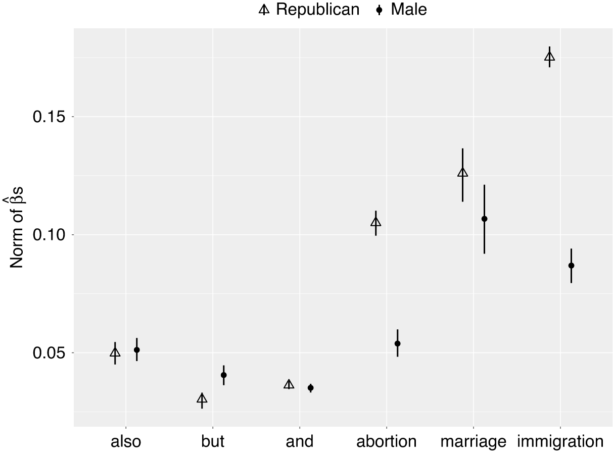
Figure 5. Differences in Word Meaning by Gender and Party
Note: Generally, different genders in the same party have more similar understanding of a term than the same gender across parties. See SM Section J for full regression output. All coefficients are statistically significant at 0.01 level.
As expected, the differences across parties and across genders, is much larger for the more political terms—relative to function words. But, in addition, embeddings differ more by party than they do by gender. That is, on average, men and women within a party have more similar understandings of the terms than men and women across parties.
The “most partisan” target in our set is immigration. Table 4 shows the top 10 nearest neighbors for each party. One reading of these nearest neighbors is that Democrats were pushing for reform of existing laws, whereas Republicans were mainly arguing for enforcement. We can corroborate this via the top nearest contexts—that is, the individual contexts of immigration—embedded using ALC—that are closest to each party’s ALC embedding of the term (see Table 5). This suggests some validity of our general approach.
Table 4. Top 10 Nearest Neighbors for the Target Term “Immigration”

Table 5. Subset of Top Nearest Contexts For The Target Term “Immigration”

Our approach is not limited to binary covariates. To illustrate, we regress the target word immigration on the first dimension of the NOMINATE scoreFootnote 10—understood to capture the liberal–conservative spectrum on economic matters (Poole Reference Poole2005). This approximates a whole sequence of separate embeddings for each speaker, approximated using a line in the NOMINATE space. We estimate the following regression:
 $$ \mathbf{Y}={\beta}_0+{\beta}_1\mathrm{NOMINATE}+\mathbf{E}. $$
We next predict an ALC embedding for immigration at each percentile of the NOMINATE score and compute its cosine similarity with a small set of hand-picked features. Figure 6 plots these results. Consistent with our results above, we observe how the predicted ALC embedding for immigration is closer to enforce and illegals at higher values of the NOMINATE score. It is closer to reform and bipartisan at lower values. The feature amend on the other hand, shows similar values across the full range.

Figure 6. Cosine Similarity (LOESS Smoothed) between Various Words and “Immigration” at Each Percentile of NOMINATE Scores
Note: We mark the median Democrat and median Republican to help calibrate the scale. See SM Section J for full regression output.

Figure 7. Norm of the British and American Difference in Understanding of “Empire,” 1935–2010
Note: Larger values imply the uses are more different. The dashed lines show the bootstrapped 95% CIs. See SM Section J for full regression output.
The Meaning of “Empire”
Recall that our plan for the second case study was to compare the embedding of Empire in the UK and US context for the period 1935–2010. In the estimation we use the top (most frequent) 5,000 tokens of the combined corpora and we estimate a 300-dimensional GloVe model and corresponding A matrix specific to the corpus. The multivariate regression analogy is
 $$ \mathbf{Y}={\beta}_0+{\beta}_1\mathrm{CongressionalRecord}+\mathbf{E}, $$
estimated for every year of the period. Interest focuses on the (normed) value of $ {\beta}_1 $
: when this rises, the use of Empire is becoming less similar across the corpora (Congress is becoming more distinctive). The time series of the
$ {\beta}_1 $
: when this rises, the use of Empire is becoming less similar across the corpora (Congress is becoming more distinctive). The time series of the $ {\beta}_1 $
s is given in Figure 7. The basic summary is that, sometime around 1949–50, there was a once-and-for-all increase in the distance between US and UK understandings of Empire. We confirmed this with a structural break test (Bai and Perron Reference Bai and Perron1998).
$ {\beta}_1 $
s is given in Figure 7. The basic summary is that, sometime around 1949–50, there was a once-and-for-all increase in the distance between US and UK understandings of Empire. We confirmed this with a structural break test (Bai and Perron Reference Bai and Perron1998).
To understand the substance of the change, consider Figure 8. We report the “most American” and “most British” (with reference to the parliaments) terms from the period on either side of the split in the series. Specifically, we calculate the cosine similarity between the ALC embedding for Empire and each nearest neighbor in the UK and US corpus. The $ x $
-axis is the ratio of these similarities: when it is large (farther to the right), the word is relatively closer to the US understanding of Empire than to the UK one. An asterisk by the term implies that ratio’s deviation from 1 is statistically significantly larger than its permuted value, p < 0.01.
$ x $
-axis is the ratio of these similarities: when it is large (farther to the right), the word is relatively closer to the US understanding of Empire than to the UK one. An asterisk by the term implies that ratio’s deviation from 1 is statistically significantly larger than its permuted value, p < 0.01.

Figure 8. UK and US Discussions of “Empire” Diverged after 1950
Note: Most US and UK nearest neighbors pre and post estimated breakpoint. * = statistically significant at 0.01 level.
The main observation is that in the preperiod, British and American legislators talk about Empire primarily in connection with the old European powers—for example, Britain and France. In contrast, the vocabularies are radically different in the postbreak period. Whereas the UK parliament continues to talk of the “British” empire (and its travails in “India” and “Rhodesia”), the US focus has switched. For the Americans, understandings of empire are specifically with respect to Soviet imperial ambitions, and we see this in the most distinct nearest neighbors “invasion,” “Soviet,” and “communists,” with explicit references to eastern European nations like “Lithuania.”
Brexit Sentiment from the Backbenches
Our goal is to estimate the sentiment of the Conservative party toward the EU in the House of Commons. First, the underlying debate text and metadata is from Osnabrügge, Hobolt, and Rodon (Reference Osnabrügge, Hobolt and Rodon2021), covering the period 2001–2019. We are interested in both major parties of government, Labour and Conservatives. We divide those parties’ MPs by role: Cabinet (or Shadow Cabinet in opposition) members of the government party are “cabinet,” and all others are “backbenchers,” by definition. We compare policy sentiment in three areas: education (where our term of interest is “education”), health (“nhs”), and the EU (“eu”).
In what follows, each observation for us is a representation of the sentiment of a party-rank-month triple toward a given term. For instance, (the average) Conservative-backbencher-July 2015 sentiment toward “health.” We describe our approach in SM E; in essence we measure the inner product between the term of interest to the aggregate embeddings of the (positive and negative) words from a sentiment dictionary (Warriner, Kuperman, and Brysbaert Reference Warriner, Kuperman and Brysbaert2013). We then rescale within party and policy area, obtaining Figure 9. There, each column is a policy area: education, health, and then the EU. The rows represent the Conservatives at the top and Labour at the bottom, with the correlation between Tory backbenchers and cabinet in the middle. We see an obvious “government versus opposition” Westminster dynamic: when Labour is in power (so, from the start of the data to 2010), Labour leaders and backbenchers are generally enthusiastic about government policy. That is, their valence is mostly positive, which makes sense given almost total government agenda control (i.e., the policy being discussed is government policy). The Conservatives are the converse: both elites and backbenchers have negative valence for government policy when in opposition but are much more enthusiastic when in government. This is true for education, and health to a lesser extent. So far, so expected.

Figure 9. Conservative Backbenchers Were Unsatisfied with Their Own Government’s EU Policy Prior to the Referendum
Note: Each column of the plot is a policy area (with the seed word used to calculate sentiment). Those areas are education (education), health (nhs), and the EU (eu). Note the middle-right plot: rank-and-file Conservative MP sentiment on EU policy is negatively correlated with the leadership’s sentiment.
But the subject of the EU (the “eu” column) is different (top right cell). We see that even after the Conservatives come to power (marked by the dotted black line in 2010), backbench opinion on government policy toward Europe is negative. In contrast, the Tory leadership are positive about their own policy on this subject. Only after the Conservatives introduce referendum legislation (the broken vertical line in 2015) upon winning the General Election do the backbenchers begin to trend positive toward government policy. The middle row makes this more explicit: the correlation between Tory leadership and backbench sentiment is generally positive or close to zero for education and health but negative for the EU—that is, moving in opposite directions. Our finding here is that Cameron never convinced the average Conservative backbencher that his EU policy was something about which they should feel positive.
A more traditional approach would be to count the number of occurrences of terms in the sentiment dictionary and assign each speech a net valence score. Figure 10 displays that result. Patterns are harder to read. More importantly, only 56% of the terms in the dictionary occur in the speeches and a full 69% of speeches had no overlap with the set of dictionary terms—and thus receive a score of 0. This contrasts with the 99% of terms in the dictionary appearing in the pretrained embeddings, allowing for all speeches to be scored. This is due to the continuity of the embedding space.

Figure 10. Replication of Figure 9 Using a Dictionary Approach
Note: The sentiment patterns are less obvious.
Advice to Practitioners: Experiments, Limitations, Challenges
Our approach requires no active tuning of parameters, but that does not mean that there are no choices to make. For example, the end user can opt for different context window sizes (literally, the number of words on either side of the target word), as well as different preprocessing regimes. To guide practice, we now summarize experiments we did on real texts. Below, we use “pretrained” to refer to embeddings that have been fit to some large (typically on-line) data collection like Wikipedia. We use “locally fit” to mean embeddings produced from—that is, vectors learned from—the texts one is studying (e.g., Congressional debates). We note that Rodriguez and Spirling (Reference Rodriguez and Spirling2022) provide extensive results on this comparison for current models; thus, here we are mostly extending those enquiries to our specific approach. Our full write up can be seen in Supplementary Materials F–H. The following are the most important results.
First, we conducted a series of supervised tasks, where the goal is to separate the uses of trump versus Trump per our example above. We found that removing stopwords and using bigger context windows results in marginally better performance. That is, if the researcher’s goal is to differentiate two separate uses of a term (or something related, such as classifying documents), more data—that is, larger contexts, less noise—make sense. To be candid though, we do not think such a task—where the goal is a version of accuracy—is a particularly common one in political science.
We contend a more common task is seeking high-quality embeddings per se. That is, vector representations of terms that correctly capture the “true” embedding (low bias) and are simultaneously consistent across similar specifications (low variance, in terms of model choices). We give many more details in the SM, but the basic idea here is to fit locally trained embeddings—with context window size 2, 6, and 12—to the Congressional Record corpus (Sessions 107–114). We then treat those embeddings as targets to be recovered from various ALC-based models that follow, with closer approximations being deemed better. As an additional “ground truth” model, we use Stanford GloVe pretrained embeddings (window size 6, 300 dimensions). We narrow our comparisons to a set of “political” terms as given by Rodriguez and Spirling (Reference Rodriguez and Spirling2022). We have five lessons from our experiments:
-
1. Pretraining and windows: Given a large corpus, local training of a full embeddings model and corresponding A matrix makes sense. Our suggested approach can then be used to cheaply and flexibly study differences across groups. Barring that, using pretrained embeddings trained on large online corpora (e.g., Stanford GloVe) provides a very reasonable approximation that can be further improved by estimating an A matrix specific to the local corpus. But again, if data are scarce, using an A matrix trained on the original online corpus (e.g., Khodak et al.’s Reference Khodak, Saunshi, Liang, Ma, Stewart, Arora, Gurevych and Miya2018 A in the case of GloVe) leads to very reasonable results. In terms of context window size, avoid small windows (of size < 5). Windows of size 6 and 12 perform very similarly to each other and acceptably well in an absolute sense.
-
2. Preprocessing: Removing stopwords from contexts used in estimating ALC embeddings makes very little difference to any type of performance. In general, apply the same preprocessing to the ALC contexts as was applied at the stage of estimating the embeddings and A matrix—for example, if stopwords were not removed, then do not remove stopwords. Stemming/lemmatization does not change results much in practice.
-
3. Similarity metrics: The conventional cosine similarity provides interpretable neighbors, but the inner product often delivers very similar results.
-
4. Uncertainty: Uncertainty in the calculation of the A matrix is minimal and unlikely to be consequential for topline results.
-
5. Changing contexts over time: Potential changes to contexts of targets is a second-order concern, at least for texts from the past 100 years or so.
Before concluding, we note that as with almost all descriptive techniques, the ultimate substantive interpretation of the findings is left with the researcher to validate. It is hard to give general advice on how this might be done, so we refer readers to two approaches. First, one can try to triangulate using various types of validity: semantic, convergent construct, predictive, and so on (see Quinn et al. Reference Quinn, Monroe, Colaresi, Crespin and Radev2010 for discussion). Second, crowdsourced validation methods may be appropriate (see Rodriguez and Spirling Reference Rodriguez and Spirling2022; Ying, Montgomery, and Stewart Reference Ying, Montgomery and Stewart2021).
Finally, we alert readers to the fact that all of our analyses can be implemented using the conText software package in R (see Supplementary Materials I and https://github.com/prodriguezsosa/conText).
Conclusion
“Contextomy”—the art of quoting out of context to ensure that a speaker is misrepresented—has a long and troubling history in politics (McGlone Reference Mcglone2005). It works because judicious removal of surrounding text can so quickly alter how audiences perceive a central message. Understanding how context affects meaning is thus of profound interest in our polarized times. But it is difficult—to measure and model. This is especially true in politics, where our corpora may be small and our term counts low. Yet we simultaneously want statistical machinery that allows us to speak of statistically significant effects of covariates. This paper begins to address these problems.
Specifically, we proposed a flexible approach to study differences in semantics between groups and over time using high-quality pretrained embeddings: the conText embedding regression model. It has advantages over previous efforts, and it can reveal new things about politics. We explained how controversial terms divide parties not simply in the way they are attached to topics of debate but in their very meaning. Similarly, we showed that understandings of terms like “empire” are not fixed, even in the relatively short term, and instead develop in line with interests in international relations. We showed that our approach can be used to measure sentiment toward policy. It is not hard to imagine other applications. For example, there is evidence that voters prefer broad-based appeals (Hersh and Schaffner Reference Hersh and Schaffner2013), but these are only possible in cases where meanings are sufficiently similar within groups. Our technique could be used to explore this tension. Similarly, what is deemed the “correct” interpretation of treaties (e.g., Simmons Reference Simmons2010) or constitutions matters. Our methods could help structure studies of these changes.
We built our framework on the ALC embedding strategy. But our general approach is not inextricably connected to this particular method for estimating contextually specific meanings. We used it because it is transparent, efficient, and computationally simple. We introduced a regression framework for understanding word meanings using individual instance embeddings as observations. This may be easily extended to more complex functional forms.
There are many potential directions for the framework; we highlight two. First, ALC assumes that the meaning of nonfocal words is essentially constant. This first-order approximation could be extended with second-order information—which words co-occur with words that co-occur with the focal words—but it is unclear how much meaning would have to change across groups for this to matter. Second, we are estimating means in high dimensions using only a few data points. This is always difficult (see Gentzkow, Shapiro, and Taddy Reference Gentzkow, Shapiro and Taddy2019), and our estimates of the norms have a finite-sample bias for rare words. Thus care is needed when comparing words or groups with substantially different amounts of available data. Future work could consider the role of term frequency in these measures of meaning.
As social scientists develop further methods to study these problems, this will sharpen questions which will in turn spur better methods. But to reiterate, technical machinery cannot, of itself, answer substantive questions. That is, claims about meaning must be validated, and the way that differences in measured quantities are interpreted will always be subject to debate. We hope that the conText model that we have laid out here can provide a useful foundation for future work.
SUPPLEMENTARY MATERIALS
To view supplementary material for this article, please visit http://doi.org/10.1017/S0003055422001228.
DATA AVAILABILITY STATEMENT
Research documentation and data that support the findings of this study are openly available at the American Political Science Review Dataverse: https://doi.org/10.7910/DVN/NKETXF.
ACKNOWLEDGMENTS
We thank audience members at the Midwest Political Science Association Annual Meeting (2021), the Political Methodology society meeting, the American Political Science Association Annual Meeting (2021), Vanderbilt University’s Data Science Institute, Princeton University, and the University of Wisconsin (Madison). We are grateful to Clark Bernier, Saloni Bhogale, Max Goplerud, Justin Grimmer, Alex Kindel, Hauke Licht, John Londregan, Walter Mebane, and Molly Roberts for comments. We also thank the editor and four excellent anonymous reviewers for their careful engagement with our work.
FUNDING STATEMENT
Work done at Princeton University is in part supported by The Eunice Kennedy Shriver National Institute of Child Health & Human Development of the National Institutes of Health under Award Number P2CHD047879.
CONFLICT OF INTEREST
The authors declare no ethical issues or conflicts of interest in this research.
ETHICAL STANDARDS
The authors affirm this research did not involve human subjects.


 Open access
Comments
No Comments have been published for this article.