


Implications
Prevalence of meta-analyses in the literature demonstrates their ability to analyze large sets of heterogeneous data. This text aims at highlighting not only the strength but also the potential pitfalls of meta-analyses in Animal Science. The most delicate steps that deserve attention are (1) the completeness of the collection of candidate publications, (2) the coding of selected data to reflect original experimental design and isolate specific experimental factors, (3) the study of the meta-design, (4) the justification for the type of effect considered for study (fixed v. random), and from a statistical standpoint, the effect of studies, and (5) the post-analytic study that most often allows the analysis to be re-run at one of the previous stages by improving the quality of the procedure.
Introduction
To achieve better supported quantitative conclusions about a research question, researchers came up with the idea of grouping published studies together. Although a wonderful idea, the question of heterogeneity across experiments arose. This concern appeared a long time ago in the medical field (Pearson, Reference Pearson1904) and then in that of agricultural field experiments (Yates and Cochran, Reference Yates and Cochran1938). The term meta-analysis came more recently from medical studies (Glass, Reference Glass1976). As showed in Figure 1, based on the exploration of the Web of Science, there has been an exponential increase in the number of publications that have applied meta-analyses in Animal Science with a progress of 15% per year. This trend, which follows with a lag of 10 to 15 years the area of medical sciences (Sutton and Higgins, Reference Sutton and Higgins2008), is likely to continue for several more years. This rapid evolution is mainly due to the growing accumulation of experimental data per topic of interest (increasing numbers of publications/topic and of measured data/publication etc.).

Figure 1 Evolution of the numbers of publications (y axis) when crossing the keywords ‘Meta-analysis x Animal’ in the Web of Science.
In Animal Science, meta-analysis has proven to be an efficient way to renew already published data by creating new empirical models, allowing progress in both understanding and prediction aspects. The progress is allowed by (1) the reduction of biases and imprecision and (2) by enlarging a priori the domain of validity of the model.
The publication of St-Pierre (Reference St-Pierre2001) was a key step in the consideration, design and development of meta-analyses in physiology and animal nutrition. Indeed, it was the first publication, in a scientific journal, addressing the main ‘ins and outs’ of meta-analysis and proposing a series of reflexions and conceptualizations relative to this issue. It highlights the importance of splitting inter- and intra-experiment variation. Logically, this work has been cited extensively in the field of Animal Science, so a landmark publication for this tool. Subsequently, Sauvant et al. (Reference Sauvant, Schmidely, Daudin and St-Pierre2008) focused on questions of good practices to be applied in meta-analysis within Animal Science: on graphical interpretation, on the choice between random and fixed effects of experiment, and on the question of interfering factors (IFs) and on that of the meta-design (see below).
The publications of St-Pierre (Reference St-Pierre2001) and Sauvant et al. (Reference Sauvant, Schmidely, Daudin and St-Pierre2008) are now, respectively, 19 and 12 years old. Since these writings, many meta-analyses have been done and published (Figure 1). Beyond these publications, meta-analyses have also proven their usefulness for updating feed unit systems. For example, the recent book ‘Feeding System for Ruminants’ (INRA, 2018) was constructed on hundreds of meta-analyses that proposed more than 500 empirical equations calculated from more than 25 databases.
Based on these years of experience, this paper will focus on further developing the definition of good practices and the limits of meta-analysis. Sauvant et al. (Reference Sauvant, Schmidely, Daudin and St-Pierre2008) proposed a heuristic cyclical generic approach with successive steps to conduct the meta-analyses that can be updated thanks to different publications on the subject and serves as a basis for the plan (Figure 2). This approach is rather similar to that proposed in Agronomy by Philibert et al. (Reference Philibert, Loyce and Makowski2012).

Figure 2 Graphical representation of the meta-analytic process, updated from Sauvant et al. (Reference Sauvant, Schmidely, Daudin and St-Pierre2008): (Pub = publication, exp = experiment, fact = factor, Int = interferent).
Specificities of meta-analyses in Animal Science
As indicated by St-Pierre (Reference St-Pierre2001) and Sauvant et al. (Reference Sauvant, Schmidely, Daudin and St-Pierre2008), meta-analyses in Animal Science are generally quite different in terms of methods and objectives from meta-analyses conducted in the medical domain. However, few meta-analyses have also been applied in Animal Science following a similar approach (Phillips, Reference Phillips2005; Hillebrand, Reference Hillebrand2009; Bougouin et al., Reference Bougouin, Appuhamy, Kebreab, Dijkstra, Kwakkel and France2014; Srednicka-Tober et al., Reference Srednicka-Tober, Baranski, Seal, Sanderson, Benbrook, Steinshamn, Gromadzka-Ostrowska, Rembialkowska, Skwarlo-Sonta, Eyre, Cozzi, Larsen, Jordon, Niggli, Sakowski, Calder, Burdge, Sotiraki, Stefanakis, Yolcu, Stergiadis, Chatzidimitriou, Butler, Stewart and Leifert2016).
In medicine, meta-analyses are mainly performed to have a more precise estimate of the effect of treatment or risk factor for disease (Haidich, Reference Haidich2010). In Animal Science, meta-analyses are mainly interested in the relations between quantitative variables to predict the average response of a dependent variable (Y), within-experiment, to one, or more, independent variables or covariables (X(s)) such as Y = f(X). To illustrate this type of objective, the variance (σ 2) of two variables Y and X is represented with circles as a Venn diagram in Figure 3, and the overlap between the two circles represent the covariance (σY.σX) (https://en.wikipedia.org/wiki/Venn_diagram). In this Figure, the two main sources of variation are distinguished for both Y and X, with the within-experiment (or intra-) variance represented below the horizontal line and the between-experiment (or inter- or across) variance above that line. This dissociation between the two sources of variance is of high importance as it allows to obtain correlation or regression coefficients specific to intra- or inter-experiment variance. Sometimes, these inter- and intra-relationships may be inversely related which can lead to difficulty in the interpretation. In such variance–covariance analysis, a benefit is that from intra-experiment covariance, one seeks to extract a generic empirical response Y = f(X) with, for example, X being a causal feeding practice which has been studied in a set of experiments. Under these conditions, what is called the experiment heterogeneity or effect corresponds to the variation of Y between studies not considered by the covariables X (cf. area ‘inter σ 2Y’ in Figure 3). The fact that the covariable is systematically calculated intra-experiment in Animal Science also constitutes a difference with the medical field where a covariable is sometimes used to explain the heterogeneity across studies (i.e. meta-regression of Borenstein et al., Reference Borenstein, Hedges, Higgins, Rothstein, Borenstein, Hedges, Higgins and Rothstein2009). Reasons for this difference will be considered further.

Figure 3 Venn diagram of meta-analytic splitting components of variance (σ 2) intra- and inter-experiment (horizontal axis) and between dependent variable Y and independent variable(s) X (Exp = experiment).
First steps in meta-analyses
Selecting the publications
One of the hallmarks of meta-analyses compared to conventional literature reviews is its comprehensiveness on a subject with an exhaustive collection and consideration of candidate publications based on a set of keywords that are closely consistent with the objectives of the work. It must start with the most generic keywords that are refined gradually to obtain a list of eligible publications. Through that phase, the reduction of the number of candidate publications may be important. For instance, d’Alexis et al. (Reference D’Alexis, Sauvant and Boval2014) conducted a meta-analysis on mixed grazing on 9 publications after starting from an initial set of 8044 references, reduced to 117 eligible candidates with ‘mixed grazing’ as a first filter. Publication filtering is the data quality step that is based on critical assessment of each of them, focusing on elements that could harm or not allow the analysis of the data based on the expertise of the analyst. This visualization step by introducing the data from a publication into a larger data set is the ultimate quality screening. One important aspect during this selection step is to explicitly mention the reasons for the exclusion at each steps of the selection process to obtain a PRISMA flow diagram (Moher et al., Reference Moher, Liberati, Tetzladd and Altman2009). This is a good practice and allows the reader to understand why some candidate articles have not been included to ensure traceability and reproducibility of the analysis.
Data structure challenges
The result of pooling publications is a table of data where rows represent treatments, while the columns consist of the measured variables and characteristics. One of the features of this data set is numerous missing data. This seriously limit the possibility of using multi-variate statistics such as principal component analysis. Therefore, analyses of Y = f(X) must be performed by successive steps on small subsets of independent variables, frequently one by one to minimize the loss of information. Moreover, in some situations, the prediction of Y must be based on several covariables to avoid the omitted-variable bias due to the fact that a significant independent covariable is not taken into account in the model. However, when more variables are included in the model, the number of observations is reduced and could become insufficient. Drawbacks of missing data are more important when complicated or expensive measures are concerned and it can limit the interest to perform meta-analysis. As an example, in a recent meta-analysis focused on grazing behavior of ruminants (Boval and Sauvant, Reference Boval and Sauvant2019), a database of 109 publications (npub), 263 experiments (nexp) and 905 treatment means (n) was gathered. The most measured behavioral item was the bite mass (npub = 65, nexp = 167 and n = 580), measured in 64% of the treatments. But, to study bite depth, the corresponding numbers were only npub = 21, nexp = 74 and n = 225. Moreover, for testing the influences of factors such as sward height (SH) or herbage bulk density (HBD), the numbers of experiments and treatments available decreased even more (nexp = 53 or 22, and n = 126 or 69, respectively) limiting the interest of the meta-analysis.
From a table of data to a database by encoding
Once all the publication’s data have been entered, we have a table of data that cannot be exploited as such. It is necessary to transform it into an organized database suited for a meta-analysis process. It includes a preliminary step of coding the data that is essential to ultimately generate new reliable and generalizable knowledge with the meta-analytic tool. Unfortunately, this phase is insufficiently depicted in most publications. Such coding will also be involved in either graphical and/or statistical procedures (Figure 2). This coding can only be successful if the person doing the meta-analysis has true expertise on the subject and aware of coding methods. To summarize, the scientific value and even the ‘art’ of meta-analyses directly depend on the quality of this coding.
A first step, whatever the objective, is to code all the publications and all the experiments (or studies) carried out in each publication. As such, this ‘experiment’ code is complete, but it contains ambiguities in the sense that it mixes experiments that may have various objectives. Therefore, for an in-depth analysis, it is necessary to code each experimental objective in a separate column. As an example, in the publication of Letourneau-Montminy et al. (Reference Letourneau-Montminy, Jondreville, Sauvant and Narcy2012) looking at phosphorus utilization by pigs, different codes were given depending on whether the authors had measured growth performance, digestibility or retention or even 2 of them or the 3. Numerous columns will be gradually added for each of these codes that correspond to a factor of variation which can be specifically studied in the meta-analysis. Otherwise, according to the objective of the work, it can be necessary to create new codes. For instance, if the objective is to study the interaction between two factors A and B, it is necessary to create, beyond coding of A and B, a new code able to consider all data candidate to study the interaction A × B. This coding step traces a quick and interesting portrait of what has been studied and vice versa what has not been studied. This is also an important step to assess the degree of validity of the empirical models proposed at the end of a meta-analytic process, study the meta-design (see below) and to model responses to various factors after having checked their mutual orthogonality (see below) (Sauvant et al., Reference Sauvant, Schmidely, Daudin and St-Pierre2008).
The meta-design
Classically, experimental conception involves careful thinking to check the independence of the studied factors (Figure 3). In meta-analysis, the structure of the data corresponds to a design which is a priori neither orthogonal (independent) nor balanced. This can lead to important statistical estimation problems. The major trap concerns collinearity between independent variables, which may bias the interpretation of results, if not carefully considered. One cannot estimate separately the effects of two variables that are highly confounded with each other. Therefore, a critical study of the meta-design is a key step in meta-analyses (Figure 2; Sauvant et al., Reference Sauvant, Schmidely, Daudin and St-Pierre2008), so only new considerations and examples will be presented here. To characterize the meta-design, several steps must take place before and after the statistical analyses.
Relations between qualitative factors and independent variables X
First, it must be checked that the experimental factors and covariables (X) are independent before interpreting them. Misuses linked with this aspect were already discussed by Sauvant et al. (Reference Sauvant, Schmidely, Daudin and St-Pierre2008) (cf. area ‘inter σ 2X’, Figure 3), but other examples are considered further.
It is particularly important to make sure that variation of continuous X is similar between categories. As an example, Letourneau-Montminy et al. (Reference Letourneau-Montminy, Cirot and Lambert2018) studied the effect of CP supply on daily water consumption in broilers of two age category (0 to 21 days and 22 to 42 days). However, the number of observations in each age was unbalanced so the range of variation in CP was different between the two age categories. This means that there is a risk that the effect of age and protein be confounded, so the two variables must not be studied together. If one will include age as a class variable in the model, the effect may be highly significant, but any conclusion based on such model would be misleading.
Relations between the quantitative independent variables X
When there is only one covariable, major aspects to be considered (histogram, study effect, leverage effects etc.) were already listed by Sauvant et al. (Reference Sauvant, Schmidely, Daudin and St-Pierre2008). The complexity increases even more when two or more independent variables are considered together, especially if their interactions are also studied (see below). In such cases, plotting independent variables against each other and quantifying their correlation are needed to assess the degree of multi-collinearity, a situation that may occur when two or more predictor variables in a regression model are redundant. This is quite common in animal nutrition especially with monogastric receiving complete diets because of feed formulation practice that involves many ratios (e.g. amino acid profile, Ca and P, dietary electrolyte balance).
In this case, it is important to carefully study the orthogonality between the candidate variables and to estimate the intra-correlation between them. For example, Daniel et al. (Reference Daniel, Friggens, Chapoutot, Van Laar and Sauvant2016) pooled experiments on dairy cows dealing with either net energy or metabolisable protein supplies to model their productive responses and to test eventual interactions between both nutrients. In this work, the intra-experiment correlation coefficient between daily net energy supply and daily metabolisable protein supply was significant (R 2 = 0.42) due to simultaneous variation of feed intake within experiment, so the coefficient of the milk response attributed to protein and that attributed to energy cannot be interpreted independently. However, when the number of experiments on a specific subject is large, it is possible to reduce this correlation by selecting only the experiments with low correlation between the two factors of interest. As an example, by selecting on the same data set experiments with low variation in intake, the correlation between net energy and metabolizable protein supplies was reduced to a non-significant correlation of 0.13 (Daniel et al., Reference Daniel, Friggens, Van Laar and Sauvant2017b). Another way to try to reduce the effect of collinearity among variables is to center the values of treatments on the mean of each experiment as it was suggested by Martineau et al. (Reference Martineau, Ouellet, Kebreab, White and Lapierre2016).
Interactions between the effects of factors or covariables X
Studying the interactions across factors or covariables is an important challenge in meta-analysis. When a database contains only experiments designed according to a factorial arrangement of treatments (2 × 2 or 2 × 3 etc.), as stated earlier, a specific coding column can be made to study the interaction and the interpretation can be based either by ANOVA or by two covariables representing measures on both factors. For instance, such an approach has been applied to study the interactions between chemical and physical fiber in cattle (Sauvant and Yang Reference Sauvant and Yang2011), and the interactions between P, Ca and microbial phytase in broilers and pigs (Letourneau-Montminy et al., Reference Letourneau-Montminy, Narcy, Lescoat, Bernier, Magnin, Pomar, Nys, Sauvant and Jondreville2010, Reference Letourneau-Montminy, Jondreville, Sauvant and Narcy2012). Unfortunately, this type of situation is rare because within a topic, the number of useable factorial experiments is generally insufficient. More generally, the purpose is to study an interaction between factors from a database where no, or only few, experiments follow a factorial arrangement of the treatments. Often, but not systematically, the code of the publications can be used to study an interaction. For instance, Boval and Sauvant (Reference Boval and Sauvant2019) studied the marginal influences of SH and HBD on bite mass through two types of independent experiments focused on either SH (nexp = 51, n = 296) or HBD (nexp = 15, n = 45) impacts. To model the interaction, a set of 30 publications (n = 339), including not only these two types of experiments but also some other experiments with both data, were selected.
Interest and risk of replacing the experiment effect by a covariable
If the inter-experiment variance is largely explained by a covariable, it corresponds a priori to a situation comparable to that of meta-regressions in medicine (Borenstein et al., Reference Borenstein, Hedges, Higgins, Rothstein, Borenstein, Hedges, Higgins and Rothstein2009). For example, we have carried out a meta-analysis of 169 experiments (420 treatments) focused on dairy cows milk yield (MY = 30.5 ± 7.0 kg/day) responses to DM concentrate supply (DMIco = 9.7 ± 0.16 kg/day). Variation inter-experiment is important (SD = 8.8 kg of MY; Figure 4) and is largely explained by the phenotypic potential of MY (MYpot) of each experiment which is a common MY value of the treatments within a given experiment (Daniel et al., Reference Daniel, Friggens, Van Laar and Sauvant2017a). In this example, the inter-experimental sum of square (SS) on MY is very high (R 2 = Inter-exp SS/total SS = 0.95) and MYpot is also highly influencing MY (inter-experiment R 2 = 0.93); based on these correlations, they have a priori a similar interest to capture inter-experiment variance.

Figure 4 Responses of dairy cows milk yield (MY) to concentrate supply.
In such a situation, the analyst has a priori the choice between considering an experiment effect or replacing it with a covariable equal to the production potential of each experiment. However, in this case to interpret the coefficients of regression, it is important to ensure that the inter-experiment covariable is not related to the independent variables (DMIco and DMIco2). Several statistical models were fitted on this data set (Table 1). When the effects of experiments (fixed (1a) or random (1b)) were replaced by the potential MY of each experiment (model (2)), the intercept became non-significant, which is logical, and the coefficients of DMIco and DMIco2 were largely different from the corresponding values of fixed (1a) and random (1b) effects assumptions. It must be reminded that the coefficients of DMIco and DMIco2 present a practical significance in terms of animal response and diet formulation (Faverdin et al., Reference Faverdin, Sauvant, Delaby, Lemosquet, Daniel and Schmidely2018). Moreover, the coefficient of DMIco2 became non-significant, and based on the RMSE, the precision of the model (2) was less. These large modifications in the values of the two coefficients of regression are mainly because there is a significant positive inter-experiment relationship between the potential MY and average level of concentrate supply (R 2 = 0.40). This inter-experiment relationship is logical in the sense that experiments that used cows with a high phenotypic potential are also using more concentrate to meet their energy requirements. Finally, when model (2) is compared to model (1a), the adjusted values of treatments are globally similar (R 2 = 0.98 and a regression not different from Y = X) with a significant remaining influence of the experiments not tackled by the covariable MYpot. Moreover, residuals are less correlated between models (1a) and (2) (R 2 = 0.47) with a significant influence of the experiments in this relationship, indicating that the covariable MYpot takes only partly into account the inter-experiment effect. Therefore, it is important to carefully check the data to avoid the consequences of a correlation between a covariable candidate for representing the experimental heterogeneity and the intra-experiment covariables. Another way to solve this type of issue would be to create sub-groups of MY. Such an approach has been performed by Huhtanen and Nousiainen (Reference Huhtanen and Nousiainen2012) with the creation of seven sub-groups having partial overlap to increase the number of observations. By this way, it was possible to check the eventual interaction between dietary response and MY.
Table 1 Results of intra-experiment fitting milk yield (MY, kg/day) response of dairy cows to concentrate supply (DMIco, g/day) and potential milk yield (MYpot)

ns = not significant.
Another important aspect concerns the formalism of the independent variables X. Indeed, these variables can be expressed as such (cf. models (1) and (2) of Table 1), or with values of practical interest. For example, we also adjusted the data with a fixed effect, as model (1a), but according to two other formalisms of DMIco: model (3) by centering X on the mean value within each experiment allows to focus on the intra-experiment relation between X and Y limiting multi-collinearity (Figure 4), and model (4) by calculating the difference between DMIco and its adjusted value corresponding to the energy balance = 0, a meaningful nutritional pivot (Daniel et al., Reference Daniel, Friggens, Van Laar and Sauvant2017a; Faverdin et al., Reference Faverdin, Sauvant, Delaby, Lemosquet, Daniel and Schmidely2018). Intercepts and coefficients of regressions are different from those of model (1a) (Table 1), and these differences can be explained. For instance, the marginal response of MY to concentrate is high (0.83 g/g DMIco) when DMIco is close to 0, but much less (0.53 g/g DMIco) when energy balance = 0. Moreover, between models (3) and (4), the adjusted (or predicted) values of treatments are similar (R 2 > 0.999, close to Y = X) and the residues are highly correlated across treatments (R 2 = 0.91). The adjusted values and the residuals of models (3) and (4) are closely related to the corresponding criteria of model (1a) (R 2 > 0.998 and R 2 > 0.84) and model (1b) (R 2 > 0.998 and R 2 > 0.89).
These results show the importance of having a close consistency between the future practical use of a model and the formalism of independent variables. In this way, models issued from published meta-analysis cannot be used without a careful consideration of their process of construction.
Exploring a database from different angle: Y as a function of X v. X as a function of Y
In some situations, the question arises whether it could be possible for the same database to be valued for different purposes according to various meta-designs, that is, for studying both intra- and inter-experiment variation if it makes sense. For example, calorimetric experiments with lactating ruminants have provided measurements for metabolizable energy (ME) and net energy (NE = ME − Heat Production = kl × ME, kl being efficiency of use of ME to milk NE). From these measurements, authors have proposed empirical models that estimate NE from ME and others have proposed empirical models that estimate ME from NE. However, these studies have been mostly performed by mixing all the available treatments without any distinction of heterogeneity factors (publication, experiment etc.). As a result, there is a certain confusion in the interpretation of the published results. This is inconvenient since the animal maintenance requirement and the efficiency of ME to NE, derived from these equations and applied in the feeding unit systems, appear sensitive to the type of statistical approach and treatment. Thus, it was suggested by Salah et al. (Reference Salah, Sauvant and Archimede2014, Reference Salah, Sauvant and Archimede2015) and Sauvant et al. (Reference Sauvant, Nozière and Ortigues-Marty2018) to apply from a same database two different approaches specific to the objective. If the aim is to estimate animal responses to ME supply (e.g. Figure 5b), then the equations should be adjusted for the effect of experiment in order to focus on the within-experiment variation, assumed to be mainly driven by the ‘push effect’ of the differences in the level of ME induced by the design. However, when the objective is to estimate animal requirement, within-experiment variance controlled by scientist is, in most cases, of limited value. This is because within an experiment, animal factors, such as BW, are made homogenous by the investigators, so that differences between treatments are only attributable to the experimental factors being studied (i.e. effect of different levels of ME). In contrast, a large variability may be expected in animals’ factors between experiments. If this ‘pull effect’ variation is sufficiently large, it is a priori of great value to deriveequations that can predict animal requirements (Figure 5a). For instance, from 87 calorimetry experiments (n = 239) on lactating cows (n = 187) and goats (n = 52), 3 modelling approaches and 4 models were compared:
(1) An inter-experiment General Linear Model (GLM, St-Pierre, Reference St-Pierre2001) procedure (Figure 5a):
calculated across experiments (1 point = average of 1 experiment, MEm is the ME maintenance requirement, NEL is milk energy and R is the body retention/mobilization of energy) within species as fixed factor without (Table 2, model 1a) or with (Table 1, model 1b) weighing each experiment as suggested by St-Pierre (Reference St-Pierre2001). Species was tested on the inter-experiment–intra-species variance considered as random (nested structure). This model could be considered as a meta-regression in the sense of medical science. $${\rm{ME/B}}{{\rm{W}}^{{\rm{0}}{\rm{.75}}}}\,{\rm{ = }}\,{\rm{Species + M}}{{\rm{E}}_{\rm{m}}}{\rm{/B}}{{\rm{W}}^{{\rm{0}}{\rm{.75}}}}{\rm{ + }}\left( {{\rm{1/}}{{\rm{k}}_{\rm{l}}}} \right){\rm{ (N}}{{\rm{E}}_{\rm{L}}}{\rm{ \,\pm\, R)/B}}{{\rm{W}}^{{\rm{0}}{\rm{.75}}}}$$
(2) An intra-experiment GLM procedure by a variance–covariance analysis with data adjusted for the fixed effect of experiment (1 point = 1 treatment) nested by species.
$${\rm{(N}}{{\rm{E}}_{\rm{L}}}{\rm{ \,\pm\, R)/B}}{{\rm{W}}^{{\rm{0}}{\rm{.75}}}}\,{\rm{ = }}\,{\rm{a}}\,{\rm{ + }}\,{{\rm{k}}_{\rm{l}}}\left( {{\rm{ME}}} \right){\rm{/B}}{{\rm{W}}^{{\rm{0}}{\rm{.75}}}}$$(3) A Mixed model procedure (covariance matrix VC) similar to model (2) except for the effect of experiment considered in this case random instead of fixed.


Figure 5 (a) Inter-experiment relationship between ME intake and the sum of net energy partitioned into milk and to/from the body (with 1 point = average of all of the treatment of one experiment); (b) intra-experiment relationship between the sum of net energy partitioned into milk and to/from the body with ME intake (with 1 point = 1 treatment). Both relationships were obtained using the same database consisting of lactating cows and goats. ME = metabolizable energy, NE = net energy, MBW = metabolic BW.
Table 2 Comparative estimations of maintenance requirements and efficiency of metabolizable energy (ME) into net energy (NE) of milk and body reserves in ruminants (kl)

1 Means (±SE).
Table 2 summarizes the estimated maintenance (MEm/BW0.75) and efficiency from ME to NE (kl) obtained from the four different models tested with data from lactating cows and goats. From these data, it is evident that the choice of the model influences these estimations: for models (1a) and (1b), differences between experiments are the outcome of physiological stages and homeorhetic regulations, while for models (2) and (3), it is a situation of adaptive response of animal to a nutritional challenge. The estimation of maintenance requirements and ME efficiency is higher with models (1a and 1b) compared to models (2 and 3). Moreover, the best precision assessed with RMSE is logically achieved for the models which adjust for the effect of experiments (2 and 3). Otherwise, if data from dry cows and dry goats are added to this lactating data set (as a mean to include data from animals fed to a level closer to maintenance), then the same models give different estimations (unpublished data). The diversity of these results highlights the importance to justify the approach chosen for estimating these key parameters of energy unit systems.
Specificity of dynamic data
Most of the publications using meta-analysis have so far mainly concerned static data (i.e. one observation (individual or group of animal) per treatment). Nevertheless, it is quite possible to apply them to dynamic/time series data where several observations may be available such as with repeated measures. It was for instance the case of published kinetics such as lactation curves (Martin and Sauvant, Reference Martin and Sauvant2002) or postprandial changes in rumen pH (Dragomir et al., Reference Dragomir, Sauvant, Peyraud, Giger-Reverdin and Michalet-Doreau2008). A difficulty related to this type of approach is that the different kinetics taken into consideration are not consistent because of the different time measurements and intervals from one publication to another. It is therefore necessary to make a preliminary adjustment of the data in order to be able to conduct the analysis. Such example can be found in Dragomir et al. (Reference Dragomir, Sauvant, Peyraud, Giger-Reverdin and Michalet-Doreau2008) in which a third-degree polynomial was fitted on the data, or in Martin and Sauvant (Reference Martin and Sauvant2002) using successive segments of the model of Grossman and Koops (Reference Grossman and Koops1988).
The assumptions of experimental heterogeneity
Definitions and basic concepts
Global considerations
The debate between the choice of considering heterogeneity across experiments as a random or fixed effect is not new. Many papers have addressed this issue, particularly in the medical field where this choice can lead to opposite important decisions, such as authorizing or not a drug to be marketed (Thompson, Reference Thompson1994; Petitti, Reference Petitti2001; Higgins et al., Reference Higgins, Thompson, Deeks and Altman2003; Borenstein et al., Reference Borenstein, Hedges and Rothstein2007). This debate reflects the fact that there is no objective (and unambiguous) method universally accepted for choosing between fixed and random effects models. In the following section, the objective is to recall the major conceptual differences between both assumptions and to illustrate some examples of practical comparison to help the reader to take an informed decision.
Random effect
Under the assumption of a random effect the heterogeneity between experiments is considered as the result of a random sampling within a large population. Experiments are therefore assumed to be independent, and they do not have to share a priori a common objective. The objective is essentially to control and model the variance related to this experimental heterogeneity in order to achieve a prediction of Y = f(X) taking into account not only the intra-experiment but also, at least partly, the inter-experiment influence (St-Pierre, Reference St-Pierre2001; Figure 3). This assumption with this choice is that the inter-experiment heterogeneity should follow a known random distribution, in preference a Gaussian one (i.e. normal). The ambition is to be able to apply the results obtained to predict or infer any new and future experiment from the entire population (= the whole area of inference). In Animal Science, many authors have conducted and published meta-analysis considering the effect of experiments as random. However, in most cases, this choice has not been clearly justified and generally only refers to St-Pierre (Reference St-Pierre2001)’s publication, in which data were randomly generated. One consequence of treating the effect of experiments as random which includes a part of the inter-experiment variance in the calculations is that it increases a priori and logically the confidence interval (CI) values of parameters as it has been systematically observed in medical field (Borenstein et al., Reference Borenstein, Hedges, Higgins, Rothstein, Borenstein, Hedges, Higgins and Rothstein2009). Additionally, it also reduces the power of the test (Hedges and Pigott, Reference Hedges and Pigott2004; Valentine et al., Reference Valentine, Pigott and Rothstein2010). This choice can therefore reduce the value of the regression for prediction purposes (see more details below) or lead to a negative conclusion of a test of a drug in medicine area.
Fixed effect
Conceptually the choice of a fixed effect corresponds to the situation of the ‘single common effect model’ frequently described in medicine (Borenstein et al., Reference Borenstein, Hedges, Higgins, Rothstein, Borenstein, Hedges, Higgins and Rothstein2009). In this case, the variation studied and tested is assumed to come a priori essentially from a sampling variability between the experiments sharing a common objective and a common response Y = f(X). It is then assumed that there is no important interfering heterogeneity on this aspect or that this heterogeneity can be controlled with an interaction between covariables and experiments. For instance, the objective can be to estimate the average impact of dietary protein supply on a given type of animal performance by selecting only experiments that were all designed to study this aspect. A logical question following this principle is what level of standardization between studies is required to conclude that heterogeneity is not interfering? In the medical field, Higgins et al. (Reference Higgins, Thompson, Deeks and Altman2003) proposed to calculate, before choosing between a random or fixed effect, an index of heterogeneity (I 2 index) which is an index of inter-experiment dispersion for the measured item. If the result is non-significant, then the heterogeneity is considered as low and a fixed effect is recommended. This method, however, is a topic of debate in medical area (Borenstein et al., Reference Borenstein, Hedges, Higgins, Rothstein, Borenstein, Hedges, Higgins and Rothstein2009), and it has been rarely applied in Animal Science (Bougouin et al., Reference Bougouin, Appuhamy, Kebreab, Dijkstra, Kwakkel and France2014). Another issue is the narrower CI interval with a fixed effect since the inter-experiment variance is ignored. However, one can also wonder if the CI obtained by this fixed effect is not artificially narrow giving a false impression of better precision.
Interpretation of the heterogeneity: difference between random and fixed effects
The distinction between fixed and random study effects in meta-analysis is similar to what can be encountered in classic experimental designs. Indeed, in a Latin square with n diets, n periods and n animals, the animal effect can be considered random if the objective is only to control its variance. In such case, the statistical test is a priori more generalizable. In contrast, if understanding differences between animals is the objective, for instance for phenotyping purpose, a fixed effect must be preferred and at this moment the CI is narrower. By analogy, in meta-analysis, the study effect would also be considered fixed if studying heterogeneity across experiments is part of the objectives. The following sentence from Van Houwelingen et al. (Reference van Houwelingen, Arends and Stijnen2002) highlights nicely the importance of this aspect in meta-analysis: ‘In the case of substantial heterogeneity between the studies, it is the researcher’s duty to explore possible causes of heterogeneity’. Comparable sentences were also published by other researchers (Greenland, Reference Greenland1987; Berlin, Reference Berlin1995)
Association between random and fixed effects to treat heterogeneity through a nested design
If within a large set of experiments, major causes of inter-experiment heterogeneity are identified and sufficiently represented, it is suggested to create subgroups of experiments based on common major causes as defined above to apply fixed effect to rank the subgroups. In this case, the inter-experiment–intra-group variance is considered as random and used as residual to test the fixed effect, through a nested model, and then it is considered as random for the F test. Thus, Bougouin et al. (Reference Bougouin, Leytem, Dijkstra, Dungan and Kebreab2016) tested influences of categorical variables of housing systems on ammonia emissions, the experiment effect being considered as random. Otherwise, several levels of nested factors can be tested; it is basically the case with the nested structure publication < experiment intra-publication < study intra-experiment, although rarely tested as such (Martineau et al., Reference Martineau, Ouellet, Kebreab, White and Lapierre2016). The nested structure can also concern factors, for example, in a meta-analysis studying interest of mixed grazing, D’Alexis et al. (Reference D’Alexis, Sauvant and Boval2014) proposed, after studying the database, the following nested structure: climate (1 df) < publications intra-climate (7 df) < replications within publication (8 df) < types of associated animals (10 df) < inter-experiment intra factors.
Examples of comparisons between random and fixed effects
To give an idea of differences induced by treating the study effect as fixed or random, it seems to us easier to briefly describe some examples.
Example 1: meta-analysis with numerous heterogeneous experiments
There were two published comparisons between the two types of effects with numerous experiments (online documents from Loncke et al., Reference Loncke, Nozière, Bahloul, Vernet, Lapierre, Sauvant and Ortigues-Marty2015 and Daniel et al., Reference Daniel, Friggens, Chapoutot, Van Laar and Sauvant2016). Additionally, Table 1 (models (1a) v. (1b)) and Table 2 (models (2) v. (3)) from the present manuscript also presented two other comparisons between the two effects. From these four examples treating numerous experiments (>30), it appeared that (1) the intra-experiment regressions and the adjusted values of the parameters were very similar; (2) the residuals were closely related and slope between residuals was not different from 1; and (3) intercept CI was systematically greater for random than fixed, whereas CI coefficients of intra-experiment regression (i.e. slopes) were very similar.
Example 2: further study of the experiment effect in the data set of St-Pierre (Reference St-Pierre2001)
St-Pierre (Reference St-Pierre2001) did a comparison between fixed and random effects on a simulated data set of 20 experiments (n = 108 treatments) where effects of experiments on intercept and slope were mutually correlated by construction. To go a bit further in this interesting work, we have reconsidered this data set by comparing four approaches:
(1) Average of separate individual fittings of the 20 experiments by 20 linear regressions (IND).
(2) GLM procedure (experiment as fixed effect) including interaction between experiments and covariable X.
(3) Mixed model with experiment effect as random with the hypothesis of ‘variance component’ (VC) structure of covariance matrix including, as model (2) an interaction between experiments and covariable as random effect.
(4) idem (id) than model (3) but with the ‘unstructured’ covariance matrix (UN).
The major results concerning this comparison are (Table 3):
A confirmation of conclusions of Example 1: adjusted or predicted values of treatments are similar between models. The mean intra-experiment slopes are similar between models 2, 3 and 4, and residuals are positively correlated (r 2 = 0.84, 0.90 and 0.98 between models 2 and 3, models 2 and 4, and models 3 and 4, respectively). Also, CIs were larger for both mixed models (3 and 4): more than two times for the intercepts but only 1.2 to 1.3 times for the slopes.
Compared to models 1 and 2, random models provide a narrower range of values for slopes across experiments (Figure 6). A major difference between fixed and random is found for experiments with two treatments, for which predicted values are very different from the average of all slopes (model 1).
Figure 6 Comparisons of values of the intra-experiment slopes (b1) with the data set of St-Pierre (Reference St-Pierre2001). For GLM, VC and UN, see Table 3.
For model 2 (i.e. fixed effect), intercept and slope are not related, whereas there is a positive correlation for random models (R 2 = 0.24 for model 3 and R 2 = 0.30 for model 4). These last results are consistent with the way the database was constructed assuming an R 2 = 0.25 between slope and intercept (St-Pierre, Reference St-Pierre2001).
Average values of residuals per experiment are equal to 0 in model 2, whereas in models 3 and 4, average values are 0.0019 (±SE, 0.031) and 0.0013 (±0.030), respectively. Moreover, independently of the mixed model considered, these average residual values per experiment are largely explained by the average values of Y and the number of treatments per experiment (Figure 7a). This confirmed that part of the inter-experiment variance of Y is found in the residual variance for model with random study effect.
Figure 7 Influence of the mean value of the dependent variable on the averaged values of the residuals per experiment in a random model (VC) for examples 2 (a) and 3 (b). Black circles are experiments with only two treatments, white circles are experiments with more than two treatments.
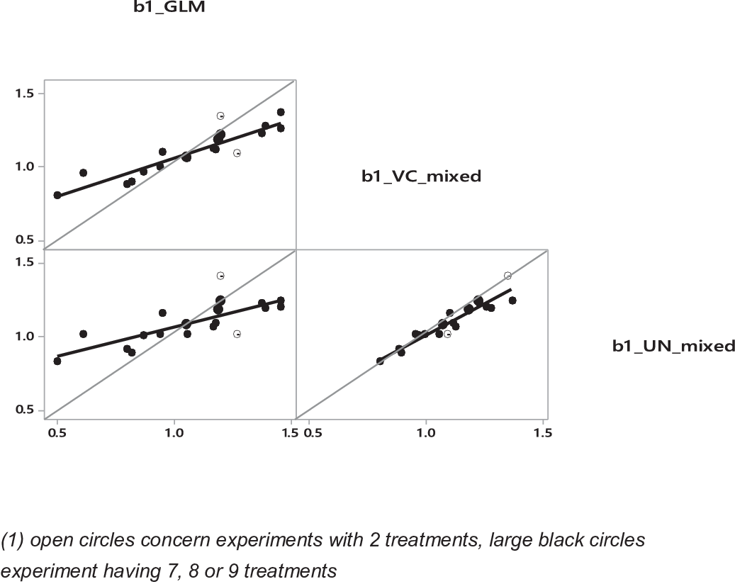

Table 3 Comparison between the major parameters with the fixed and mixed models

1 Means (±SE).
Example 3: experiment effects and post analytical study in a practical situation
As the previous example using data from St-Pierre (Reference St-Pierre2001) was a theoretical one, we did a similar approach with data from Figure 4, in which MY responses to concentrate supply in dairy cows were studied. The comparison between models 1a (fixed) and 1b (random, VC) is presented in Table 1, and major differences and similarities with example 2 are:
– The mean slopes of individual experiments were highly correlated (R 2 = 0.99) between random and fixed, and the relation was not different from Y = X. This result contrasts with comparison made in example 2 (see Figure 6). Potential interaction between experiment and dependent variable X may explain this discrepancy. Further comparative studies are warranted to conclude on this aspect.
– Average residuals between models (1a) and (1b) were equal, and treatment residuals were highly correlated across treatments (R 2 = 0.99 with slope not different from 1). However, the differences between treatment residuals of random and fixed effects were related to MY as illustrated in Figure 8. Between-experiment, this relationship was positive but within-experiment, the relationship was negative. This clearly highlights differences in how experiments heterogeneity is considered between random model and fixed model.
Figure 8 Relationships in lactating cows between milk yield (MY) and difference between residuals of random and fixed models in kg MY/day.
– Average residuals per experiment obtained with the GLM model (Table 1, model 1a) were all 0, whereas with the mixed model (Table 1, model 1b), average residuals per experiment were different from 0 (0.004 ± 0.096). These averages were correlated with average MY of experiments; moreover, this relationship was highly influenced by the number of treatments per experiment (Figure 7b) as observed with the data from St-Pierre (Figure 7a).

As a partial conclusion, it appears that, for examples 2 and 3, part of the inter-experiment variance of Y is left in the residual variance of the random model. It should however be noted that this variance represents only less than 10% of the total residual variance of the model. Consequently, the type of model (random or fixed) would lead to the same conclusion with respect to which experiments may be identified as outlier due to high studentized residual values (Sauvant et al., Reference Sauvant, Schmidely, Daudin and St-Pierre2008).
Example 4: case of a curvilinear response and an unbalanced design
Loncke et al. (Reference Loncke, Nozière, Bahloul, Vernet, Lapierre, Sauvant and Ortigues-Marty2015) has studied the flux of β-hydroxybutyrate from the liver in ruminants as a function of energy balance. The database used included 6 experiments with dairy cows (n = 12), 9 with growing ruminants (n = 22) and 8 with non-productive ruminants fed close to maintenance (n = 20). The intra-experiment response was curvilinear, and the size of the quadratic term was influenced by the choice of treating the experiment effect as fixed or random (Figure 9). The largest difference was found in the adjustment for the dairy cow group, in which predicted values at low or high energy balance were higher in the random model than in the fixed model. One explanation of these differences between fixed and random could be related to the unbalanced number of observations in each physiological status (Figure 9).

Figure 9 Observed and adjusted net hepatic release of β-hydroxybutyrate relative to energy balance for dairy cows (continuous) growing cattle (short dashes) and maintenance (long dashes). The thick lines represent the adjustment with the fixed model, and thin lines represent the adjustment with the random model (from Loncke et al. Reference Loncke, Nozière, Bahloul, Vernet, Lapierre, Sauvant and Ortigues-Marty2015; reproduced with permission).
Interfering factors
The issue of IFs is also sometimes an object of debate (Sauvant et al., Reference Sauvant, Schmidely, Daudin and St-Pierre2008). Originally, the research for IF consisted of investigating whether qualitative factors, or incomplete variables (because of missing values), that are, for this reason, not incorporated into the adjusted statistical model, could explain a significant part of the variation in the data. More precisely, when the best independent X variable(s), considered as primary driver(s), has been found, it is advisable to evaluate if any secondary variables could influence the response equation. The study of the IF can be carried out at various levels: (1) on the Least square means (LSMeans); (2) on slopes of the intra-experiment relationships (within-study slopes) and (3) in the residual variance.
A systematic study of IF allows one to gain more knowledge from the data. Some examples of this approach can be found in the literature (Loncke et al. Reference Loncke, Ortigues-Marty, Vernet, Lapierre, Sauvant and Nozière2009, Reference Loncke, Nozière, Bahloul, Vernet, Lapierre, Sauvant and Ortigues-Marty2015 and Reference Loncke, Nozière, Vernet, Lapierre, Bahloul, Al-Jammas, Sauvant and Ortigues-Marty2020; Agastin et al. Reference Agastin, Sauvant, Naves and Boval2014). In the meta-analysis of Loncke et al. (Reference Loncke, Nozière, Bahloul, Vernet, Lapierre, Sauvant and Ortigues-Marty2015), response equations to predict hepatic uptake/release of ketogenic nutrients in response to their supply to the liver were obtained using published data from the FLORA database (FLuxes of nutrients across Organs and tissues in Ruminant Animals; Vernet and Ortigues-Marty, Reference Vernet and Ortigues-Marty2006). In this meta-analysis, the study of IF revealed that response equations were significantly affected by other nutrients or by diet characteristics. For example, it was shown that the hepatic release of glucose was related to the net portal appearance of nitrogen (Loncke et al., Reference Loncke, Nozière, Vernet, Lapierre, Bahloul, Al-Jammas, Sauvant and Ortigues-Marty2020), but for a same level of nitrogen (LSMeans), the release of glucose increased logically with the dietary starch concentration.
In general, it is necessary to consider all factors and variables as potential IF and to test their influence on the parameters (LSMeans, residuals and within-study slopes); Loncke et al. (Reference Loncke, Ortigues-Marty, Vernet, Lapierre, Sauvant and Nozière2009, Reference Loncke, Nozière, Bahloul, Vernet, Lapierre, Sauvant and Ortigues-Marty2015 and Reference Loncke, Nozière, Vernet, Lapierre, Bahloul, Al-Jammas, Sauvant and Ortigues-Marty2020) tested about 50 IFs for each equation published. The major objective of the analysis of potential IF aims to evaluate if the main independent variables (i.e. the identified primary drivers) have consistent effects across various scenarios (no IF) or if those effects are function of specific conditions (presence of IF). When an IF is identified, it is recommended to try to include it in the model, as a covariable or cofactor, and to evaluate if this inclusion enhances the model adjustment without over-complicating the model interpretation or the use of the model in practical situation. So, in order to be as exhaustive as possible in the study of potential IF, it is important to build a complete data set. Indeed, some variables may seem secondary at first but may be relevant for such test and thus it is therefore highly advisable to enter all reported variables from a selected publication into the database.
Evaluation of models obtained from meta-analysis
A priori the validation of a model obtained from a meta-analysis has to be conducted on an exogenous data set that did not contribute to the model adjustment as it has been performed, for example, by Ellis et al. (2016) to predict hepatic blood flow from intake level. This evaluation has been frequently based on the study of the structure of the residuals, of the Bayesian Information Criterion and on the Concordance Correlation Coefficient. However, this is a difficult approach since such comparison must be done on a data set with very similar characteristics in terms of experimental factors (number of factors, range), of meta-design and of range of data studied (both dependent and independent variables). Alternatively, cross-validation approaches can be performed. This consists of splitting the data set in subgroups which are successively removed to re-run the model. It seems that when the data set is large and the objectives of experiments are homogeneous, such cross-validation is satisfying (Huhtanen and Nousiainen, Reference Huhtanen and Nousiainen2012). Another way to simply proceed a cross-validation with large data sets is to randomly select sub-parts of the database which can be used to assess the robustness of the model on these subparts (this is sometimes called k-fold cross validation). Thus, in the work of Bougouin et al (Reference Bougouin, Appuhamy, Ferlay, Kebreab, Martin, Moate, Benchaar, Lund and Eugène2018), only one sub-data set corresponding to 30% of the collected data was considered for the evaluation procedure. Such approaches are however questionable for data rarely measured for reasons of cost or technical difficulties. In fact, if the recommended principle of exhaustive data collection is applied to strengthen the conclusions, there is a priori no other available data. In this context of completeness, from our experience, it seems that the evaluation of the validity of the model lies rather in the careful study of the representativeness of the factors collected and of the data used for the meta-analysis. In particular to what extent the factors and data used are representative of what is observed in the field in terms of plausible and possible ranges? These aspects are frequently neglected despite they are strong determinants of practical validity of a meta-analytic work.
The necessity of having an evaluation phase and the way of conducting it can be different in meta-analysis according to the assumption of either random or fixed effect and if several levels of organization are considered. For a fixed effect, if specifications are well respected, the model can be considered as auto-evaluated for its field of data and level of organization. However, risks of strong biases exist when several empirical models based on fixed effect and developed at a level n on homogeneous and well-focused groups of experiences are used to model the multiple responses of a system at level n + 1. Thus, in the recent INRA Feed Unit System for Ruminants (INRA, 2018), specific coding of sub-bases of experiments having the same objective allowed to model fairly accurately the digestive influences in cattle of various specific dietary factors such as protein, starch, cell wall, fatty acids etc. (Sauvant and Nozière, Reference Sauvant and Nozière2016). However, such an approach required to carefully check the consistency of these empirical models issued from entirely different nutritional contexts before integrating them into a common model of digestion subsequently included into a Feed Unit System (INRA, 2018). The consistency of these equations and their collective evaluation was checked on a digestive mechanistic model that was calibrated on structural equations of fluxes derived from meta-analysis of the literature (Sauvant and Nozière, Reference Sauvant and Nozière2012 and Reference Sauvant and Nozière2016).
The futures of meta-analysis
The future of meta-analyses in Animal Science will depend on their ability to generate progress. Until now, only few links have been established between meta-analyses and systemic approach, while they could be particularly useful to help understanding emerging properties of complex systems. This complexity relies to the structure of the system and to the relationships between its main elements and between its various levels of organization. Meta-analyses can therefore be applied to understand the role of multiple scales in the spatiotemporal organization of systems. They can help to highlight the key relationships associating the different elements and scale levels as well as the diversity of situations and their main factors of variation.
One of the main challenges of meta-analysis concerns its combination with mechanistic modeling. Proposals remained rare in this area. For large mechanistic models, Sauvant and Martin (Reference Sauvant, Martin and Kebreab2004) have suggested to apply meta-analyses at the two different phases of construction and evaluation of the model. At the underlying level, meta-analysis of a first database allows one to obtain realistic values for the key basic parameters and relationships used to build the mechanistic model. At the most integrated level, meta-analysis of a second database, obtained at a level where the considered system is only a subsystem, allows one to assess the global validity of the model. Other synergies have been proposed between mechanistic modeling and meta-analytic approaches. Thus, it is possible to build mechanistic models applying a top-down approach by using intra-experiment regressions issued from meta-analyses as ‘structural equations’ to adjust values of the underlying parameters related to flows and compartments. Such approach has already been used to construct a simple mechanistic model of fiber digestion in the rumen. Another and more sophisticated example of this approach was carried out by Bahloul (Reference Bahloul2014) with a mechanistic model of metabolic fluxes in the liver. The domain of validity of such models is directly related to the representativity of data included in the meta-analysis and thus used for the calibration of the structural equations integrated into the mechanistic model. Recently, two interesting reviews took the opportunity of the ‘big data wave’ to broaden the thinking around modeling applied to Animal Science (Tedeschi, Reference Tedeschi2019; Ellis et al., Reference Ellis, Jacobs, Dijkstra, van Laar, Cant, Tulpan and Ferguson2020). In this perspective, meta-analyses which can be seen as data-driven model have their entire place when basic data are heterogeneous.
Data collected in the domain of Livestock Farming System are rather heterogeneous because they come from many different sources and time frequencies (Gonzalez et al., Reference Gonzalez, Kyriazakis and Tedeschi2018). In this context, empirical models obtained from meta-analyses could offer a possibility for real-time diagnosis. In addition, it is likely that meta-analysis will highlight some key features that could help progress in technology to evolve in the right direction. Genomics is another fast growing field of research which may benefit from meta-analytic approaches. So far, the information is generally sufficiently homogeneous and standardized to be processed by multivariate statistical analysis methods. It is possible that the search for ever greater integration of data will require specific processes of heterogeneous data fusion using methods already applied in the context of meta-analysis (Zhao et al., Reference Zhao, Sauvage, Zhao, Bitton, Bauchet, Liu, Huang, Tieman, Klee and Causse2019).
In a certain way, meta-analysis applied to Animal Science is progressing at a rate equivalent to that of the medical field, but with a lag of several years, which can be explained in large part by a much higher investment in Health Science research. This trends is now continuing, for instance the new paradigm of the Bayesian approach applied to meta-analysis has been developing for several years (Cummings, Reference Cumming2014; Kruschke and Liddell, Reference Kruschke and Liddell2018) with only few examples in Animal Science so far (Moraes et al., Reference Moraes, Kebreab, Firkins, White, Martineau and Lapierre2018). This approach largely renewed the concepts of model interpretation and evaluation, and this era is just now beginning in Animal Science.
Another practical consideration within Animal Science that may increase interest in meta-analyses in the future: some experimental techniques are considered as too invasive for the animals and will most likely not be authorized to be practiced any more (e.g. digestive cannulas). Consequently, published data obtained with these techniques have a priori an increased scientific value and the challenge will be to interpret them with great completeness by meta-analysis.
In the longer term, one of the challenges of meta-analysis will be related to the possibility of automating some of the key steps using artificial intelligence methods. However, hopefully humans will remain masters of the game thanks to their intelligence and their imagination.
Conclusions
The large number of publications using meta-analysis shows that it is a widely accepted and applied method in Animal Science, especially in nutrition. The methods applied have remained largely unchanged, but the required levels of reporting and traceability have evolved, and this has resulted in greater transparency, with hopefully a better repeatability between analysts. These requirements relate to the choice of the selected publications, as this defines the degree of representativeness of the work with respect to the applications, to the construction and the coding of the database, and to the study of the meta-design. It also relates to the systematic analysis of IFs in situations where many candidate independent variables are available.
The debate about the choice between fixed and random effects is evolving, and the selection of fixed/random should flow from the carefully considered objective of the meta-analysis. Our comparisons show that in most situations, the adjusted values are the same and ultimate conclusions are not influenced by this choice. In concrete terms, it is mainly the partition of variance across the effects which seems to be altered by the choice. One promising aspect of the development of meta-analyses is related to their implications in other modern approaches such as systemic and mechanistic modeling approaches. One of the future challenge for meta-analyses will be to demonstrate their usefulness in the development of precision livestock farming as well as in the processing of large, and potentially heterogeneous, data sets. Otherwise, until now, meta-analysis has mainly been applied to treatments that represent averages of several individuals. It seems that, given growing interest in phenotype studies, it would be desirable to evaluate the advantages and limits of meta-analyses to interpret individual laboratory databases by grouping the results of various experiments in which the measured characters are not systematically the same.
Acknowledgements
This review was written following the 9th ‘Workshop on Modeling Nutrient Digestion and Utilization in Farm Animals’. The authors want to thank the organizers, in particular Izabelle Teixeira and Luciano Haushild. They also want to express their gratitude to the colleagues who contributed in the reviewing and scientific editing of this article.
D. Sauvant 0000-0002-2925-5547
Declaration of interest
None.
Ethics statement
This review did not require any ethical approval.
Software and data repository resources
None.


