


1. Introduction
Iceberg calving, the process of ice separating from a glacier’s terminus, is a significant source of mass loss from Antarctica and Greenland (Depoorter and others, Reference Depoorter, Bamber, Griggs, Lenaerts, Ligtenberg, van den Broeke and Moholdt2013; Rignot and others, Reference Rignot, Jacobs, Mouginot and Scheuchl2013; Aschwanden and others, Reference Aschwanden2019; Greene and others, Reference Greene, Gardner, Schlegel and Fraser2022). When calving events occur, upstream ice flow can be affected through structural changes at the ice front and increase rates of discharge to the oceans (Rückamp and others, Reference Rückamp, Neckel, Berger, Humbert and Helm2019; Greene and others, Reference Greene, Gardner, Wood and Cuzzone2024). Reliably accounting for mass loss through calving is, therefore, an essential component in the numerical modelling of Antarctic ice sheets and glaciers. However, as there is still no consensus on the best way to do this, the process of calving remains a major source of uncertainty in future sea level rise projections (Bulthuis and others, Reference Bulthuis, Arnst, Sun and Pattyn2019; Alley and others, Reference Alley2023; Seroussi and others, Reference Seroussi2023).
There exists a need to numerically represent calving in a simple, computationally inexpensive manner that can be employed in large-scale modelling of ice sheets and glaciers over long timescales. Despite the complexity of calving processes, correlations between calving rates and simple glacial properties (for example including geometry and buoyancy conditions) have been observed in nature (Benn and others, Reference Benn, Warren and Mottram2007). Calving is, therefore, often parameterised in large-scale models under the assumption that a primary mechanism may control the rate of iceberg calving, though such parameterisations generally rely upon empirical relationships which are often poorly constrained by observational data in both space and time. However, the recent availability of high-resolution satellite derived datasets detailing glacier geometry (Howat and others, Reference Howat2022a) and ice-flow velocity (e.g. ENVEO and others, Reference Wuite, Hetzenecker, Nagler and Scheiblauer2021) offers an invaluable opportunity to add better constraint to such relationships and improve confidence in assessing their applicability in varying regions and over different time periods. Further, as the derivation of calving parameterisations are often based upon data from either a single glacier or a limited number of glaciers, some parameterisations require tuning within a numerical modelling framework in order for the observed evolution of calving front positions to be reasonably reproduced when tested over a wider range of real-world geometries (Choi and others, Reference Choi, Morlighem, Wood and Bondzio2018; Amaral and others, Reference Amaral, Bartholomaus and Enderlin2020; Wilner and others, Reference Wilner, Morlighem and Cheng2023).
Some of the earliest attempts to parameterise calving considered relationships between calving rate and terminus properties including cliff height, ice thickness and water depth. These were derived through theoretical studies (Reeh, Reference Reeh1968; Fastook and Schmidt, Reference Fastook and Schmidt1982) and through the evaluation of observational data (Brown and others, Reference Brown, Meier and Post1982, Reference Brown, Sikonia, Post, Rasmussen and Meier1983; Sikonia, Reference Sikonia1982). Although observations appeared to show that a strong correlation with calving rate existed for both ice thickness and terminus water depth (Brown and others, Reference Brown, Meier and Post1982), the derived correlations may have been incidental due to a lack of assessed datasets (Pelto and Warren, Reference Pelto and Warren1991) or due to the focus being placed on glaciers holding a steady terminus position rather than being in a retreat phase (Van der Veen, Reference Van der Veen1996).
Following further investigation, the proportionality of the correlation between calving rate and water depth was shown to vary greatly between glaciers in different regions (Pelto and Warren, Reference Pelto and Warren1991; Haresign, Reference Haresign2004). This may not be a surprising result, as the physical explanation behind the correlation between water depth and calving rate is not entirely clear; however, links to ice thickness and terminus cliff height are more coherent.
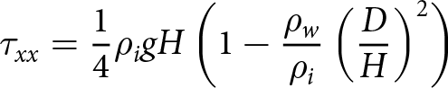
Calving may be considered to be driven by horizontal deviatoric stress τxx, at the ice front, which can be estimated through assessing the balance of vertically integrated stress in the ice column and the ocean pressure acting at the ice front (Van der Veen, Reference Van der Veen1996). This force balance approach yields an expression for horizontal deviatoric stress which is dependent on simple geometric parameters only as
 \begin{equation}
\tau_{xx} = \frac{1}{4} \rho_i g H \left(1-\frac{\rho_w}{\rho_i}\left(\frac{D}{H}\right)^2\right)
\end{equation}
\begin{equation}
\tau_{xx} = \frac{1}{4} \rho_i g H \left(1-\frac{\rho_w}{\rho_i}\left(\frac{D}{H}\right)^2\right)
\end{equation}where ρi and ρw are the densities of ice and seawater respectively, g is the gravitational constant, H is the ice thickness and D is the submerged depth of the ice. This expression assumes that tangential deviatoric stress at the terminus is negligible. In the circumstance of a floating terminus and assuming uniform densities of ice and ocean water, Eqn (1) can be reduced and the deviatoric stress can be written as proportional to the sub-aerial height of the ice front
 \begin{equation}
\tau_{xx} = C H_c
\end{equation}
\begin{equation}
\tau_{xx} = C H_c
\end{equation}where C is a constant and Hc is the sub-aerial cliff height at the terminus.
Driven by extensional stress, a primary mechanism of calving is the formation and propagation of crevasses (Benn and others, Reference Benn, Warren and Mottram2007). The basis of calving parameterisations driven by this mechanism is that full thickness penetration of crevasses may occur once a threshold stress has been met. One approach to implementing this is by estimating the location of crevasse formation and depth of propagation using a zero stress criterion (Nye, Reference Nye1957) which has been investigated in numerous studies (e.g. Benn and others, Reference Benn, Warren and Mottram2007, Reference Benn2023; Nick and others, Reference Nick, Van der Veen, Vieli and Benn2010; Pollard and others, Reference Pollard, DeConto and Alley2015; Todd and others, Reference Todd2018). Alternatively, crevasses which ultimately lead to calving may be initiated at the location of maximum tensile stress in the near-terminus region (Pralong and others, Reference Pralong, Funk and Lüthi2003; Pralong and Funk, Reference Pralong and Funk2005). Mercenier and others (Reference Mercenier, Lüthi and Vieli2018) derived calving rates based on terminus ice thickness considering a predicted time to failure following crevasse formation under this scenario. It follows that the magnitude of maximum tensile stress and consequent time to failure may be reasonably indicated by the horizontal deviatoric stress at the terminus (Eqn (2)).
Links between glacier cliff height and calving rates have also been explored based upon the theorised structural shear failure of ice when a threshold terminus cliff height is reached (Bassis and Walker, Reference Bassis and Walker2012; Ultee and Bassis, Reference Ultee and Bassis2016; Bassis and Ultee, Reference Bassis and Ultee2019; Clerc and others, Reference Clerc, Minchew and Behn2019; Parizek and others, Reference Parizek2019; Bassis and others, Reference Bassis, Berg, Crawford and Benn2021). Piecewise linear (DeConto and Pollard, Reference DeConto and Pollard2016; DeConto and others, Reference DeConto2021) and power law (Schlemm and Levermann, Reference Schlemm and Levermann2019; Crawford and others, Reference Crawford, Benn, Todd, Åström, Bassis and Zwinger2021) relationships between cliff height and calving rates have been proposed, requiring the exceedance of a threshold cliff height before calving is assumed to occur.
Antarctica’s ice mass holds the equivalent of 57.9 m in global mean sea level rise (Morlighem and others, Reference Morlighem2020) and so these relationships are significant as should threshold cliff heights be exposed, the theorised resultant high calving rates could lead to a significant increase in Antarctica’s near-future contribution to rising sea levels. Of particular note is the idea that the exposure of tall ice cliffs could lead to unstable terminus retreat, a process termed Marine Ice Cliff Instability (Bassis and Walker, Reference Bassis and Walker2012; DeConto and Pollard, Reference DeConto and Pollard2016). The findings of DeConto and Pollard (Reference DeConto and Pollard2016) suggested that by the end of the century, Antarctica could contribute in excess of 1 m to global sea level rise should such an unstable retreat process be proven. However, the calving parameterisation that was implemented by the authors was not well constrained by observational data either spatially or temporally. Without sufficient constraint of calving rates against real-world observations, the timescales and magnitudes of future ice discharge from Antarctica remain highly uncertain. Despite this, abundant remote-sensing data from recent decades, in particular the high-resolution digital elevation models from the Reference Elevation Model of Antarctica (REMA) (Howat and others, Reference Howat, Porter, Smith, Noh and Morin2019, Reference Howat2022a), provide a great opportunity for this to be re-assessed.
In reality, calving may occur as a result of the combined effects of both tensile and vertical shear stresses (Bassis and Walker, Reference Bassis and Walker2012) and the overall height of the ice cliff may influence which mode leads to failure (Schlemm and Levermann, Reference Schlemm and Levermann2019). The underlying theme of these stress-based calving parameterisations, regardless of the physics deemed responsible for calving, is that higher stresses are proportional to higher calving rates.
In this study, we make use of high-resolution observational data from 15 tidewater glaciers around the Antarctic Peninsula to assess the relationship between sub-aerial cliff height and calving rate. Due to the coverage and quality of data, we assess a 9 year time period between 2015 and 2023. We consider that the sub-aerial terminus cliff height may be considered a proxy for the magnitude of either horizontal deviatoric stress (Eqn (2)) or vertical shear stress and that higher stresses may result in higher calving rates. We apply suitable spatial and temporal averaging of both sub-aerial cliff height and calving rate to assess this relationship and arrive at a cliff height dependent calving parameterisation which is representative of the long-term calving behaviour of tidewater glaciers in the Antarctic Peninsula.
2. Study area
The Antarctic Peninsula is a mountainous region extending north from the Antarctic continent towards the southern tip of South America (Fig. 1). In the south of the peninsula, glaciers flow primarily into ice shelves whereas more tidewater glaciers are found further north. Significant glacier retreat has been observed around the Antarctic Peninsula since the 1950s (Cook and others, Reference Cook, Fox, Vaughan and Ferrigno2005) and in recent decades, 14% of the Antarctic Ice Sheet’s total contribution to global sea level rise came from the region (Otosaka and others, Reference Otosaka2023).
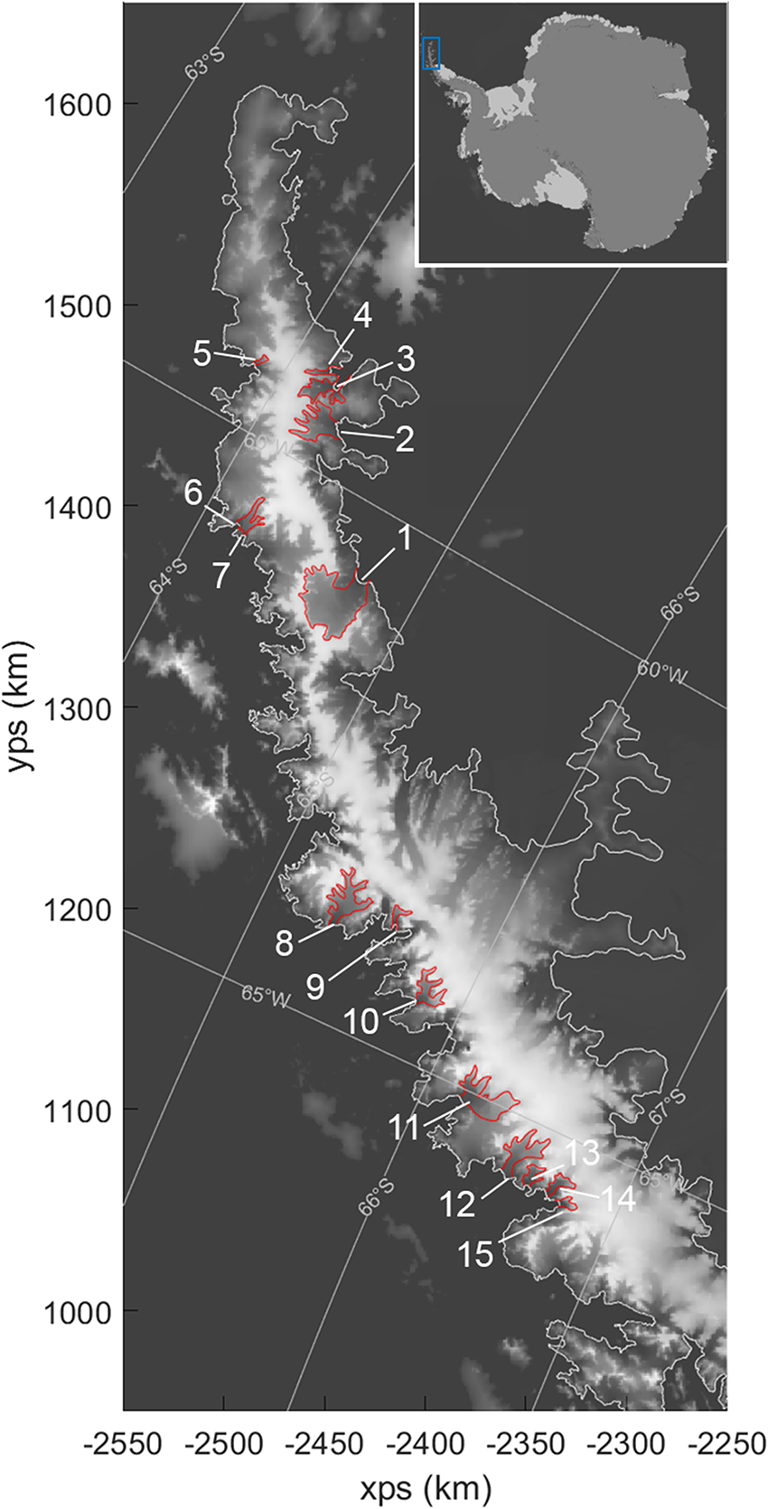
Figure 1. The study area covers the northern region of the Antarctic Peninsula, shown here on the Reference Elevation Model for Antarctica mosaic hill shade (Howat and others, Reference Howat2022b) in polar stereographic projection. Latitude and longitude lines are also plotted for reference. The white line shows the estimated grounding line position (Morlighem, Reference Morlighem2022). The assessed glaciers are outlined in red with the labelled numbers corresponding to the names and details of each glacier given in Table 1.
We focused on the northern region of the Antarctic Peninsula and considered glaciers where buttressing ice shelves and land-fast sea ice, which can influence calving behaviour (e.g. Mitcham and others, Reference Mitcham, Gudmundsson and Bamber2022; Ochwat and others, Reference Ochwat2024; Parsons and others, Reference Parsons, Sun, Gudmundsson, Wuite and Nagler2024), were not present during the time period covered by the datasets that are fundamental to the study (Howat and others, Reference Howat, Porter, Smith, Noh and Morin2019, Reference Howat2022a). The quality and availability of data (see Table 1) led to the selection of 15 tidewater glaciers for analysis (Fig. 1), the characteristics of which are given in Table 1. As the assessed glaciers cover a range of properties, this selection is anticipated to be representative of other tidewater glaciers in the region.
3. Datasets
We make use of a wealth of high-resolution data products timestamped between October 2014 and September 2023 (Figure 2) to capture spatial and temporal variation in sub-aerial cliff height and calving rate at multiple tidewater glaciers. The datasets fundamental to this study are digital elevation models, used to determine the glacier terminus positions and cliff heights, and velocity maps which are required in the calculation of calving rates.
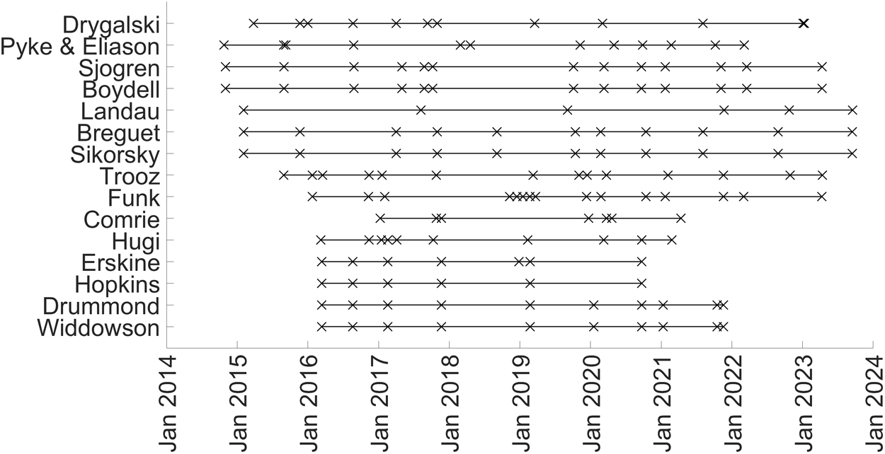
Figure 2. The dates that digital elevation models were available for each of the studied glaciers are represented by the black crosses. The lines show the overall extent of the assessed time period for each glacier, which was bound by the first and last available digital elevation models.
Digital elevation models were obtained from timestamped strips from the Reference Elevation Model for Antarctica (Howat and others, Reference Howat, Porter, Smith, Noh and Morin2019, Reference Howat2022a). These models are extracted from pairs of sub-metre resolution Maxar satellite imagery and are defined at 2 m spatial resolution. In the processing phase, each strip was vertically registered to satellite altimetry measurements from Cryosat-2 and ICESat, resulting in absolute uncertainties of <1 m. The digital elevation models are referenced to the WGS64 ellipsoid and were corrected for the geoid using values from BedMachine v3 (Morlighem and others, Reference Morlighem2020; Morlighem, Reference Morlighem2022).
Monthly averaged ice velocity maps at 200 m grid spacing were obtained from ENVEO. The maps were derived from successive Sentinel-1 interferometric wide single look complex image pairs (2014–23) using a combination of coherent and incoherent offset tracking techniques (Nagler and others, Reference Nagler, Rott, Hetzenecker, Wuite and Potin2015, Reference Nagler, Wuite, Libert, Hetzenecker, Keuris and Rott2021; ENVEO and others, Reference Wuite, Hetzenecker, Nagler and Scheiblauer2021).
4. Methodology
The difference between the ice-flow speed and the change in terminus position over time is the rate of frontal ablation, which collectively describes the processes of iceberg calving and subaqueous melt (Truffer and Motyka, Reference Truffer and Motyka2016). From the observational datasets, we could make no distinction between these two processes, however, we considered that melt rates in the Antarctic Peninsula are expected to be orders of magnitude lower than the total frontal ablation rates (Dryak and Enderlin, Reference Dryak and Enderlin2020) and, therefore, assumed that calving is the dominant process in frontal ablation. The calving rate c can, therefore, be written as
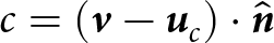 \begin{equation}
c = (\boldsymbol{v}-\boldsymbol{u}_c) \cdot \hat{\boldsymbol{n}} \\
\end{equation}
\begin{equation}
c = (\boldsymbol{v}-\boldsymbol{u}_c) \cdot \hat{\boldsymbol{n}} \\
\end{equation} where v is the material velocity of the ice, uc is the velocity of the calving front, i.e. the rate by which the position of the calving front changes over time, and  $\hat{\boldsymbol{n}}$ is a (horizontal) unit normal vector to the calving front.
For the purpose of incorporating calving in continuous ice-flow models for long-term modelling of glaciers, we were interested in the time-averaged pattern of calving rather than in capturing individual calving events. To remove the abrupt advance-retreat oscillation due to individual calving events, we applied a multiple-year window to derive the long-term trend of the ice front calving rate. As such, seasonal variation in calving rates, for example due to the impacts of melange buttressing (e.g. Greene and others, Reference Greene, Young, Gwyther, Galton-Fenzi and Blankenship2018; Kneib-Walter and others, Reference Kneib-Walter, Lüthi, Moreau and Vieli2021; Gomez-Fell and others, Reference Gomez-Fell, Rack, Purdie and Marsh2022) or enhanced subaqueous melt rates (e.g. Sciascia and others, Reference Sciascia, Straneo, Cenedese and Heimbach2013; Wood and others, Reference Wood2018), is also neglected. The results of cliff heights and calving rates presented in this study are, therefore, assessed over a 3 year average moving window.
Similarly, it was necessary to incorporate spatial averaging in order to capture the variability in terminus position change, cliff height and flow speed over a glacier’s width. We, therefore, drew a rectilinear box over the outlet region of each glacier, sub-dividing this into ten equally spaced segments and aligning with the fjord geometry and direction of ice flow (Fig. 3). The box segments were defined at a length that covered the maximum change in terminus positions over the assessed time period, with the terminus positions digitised from each digital elevation model.
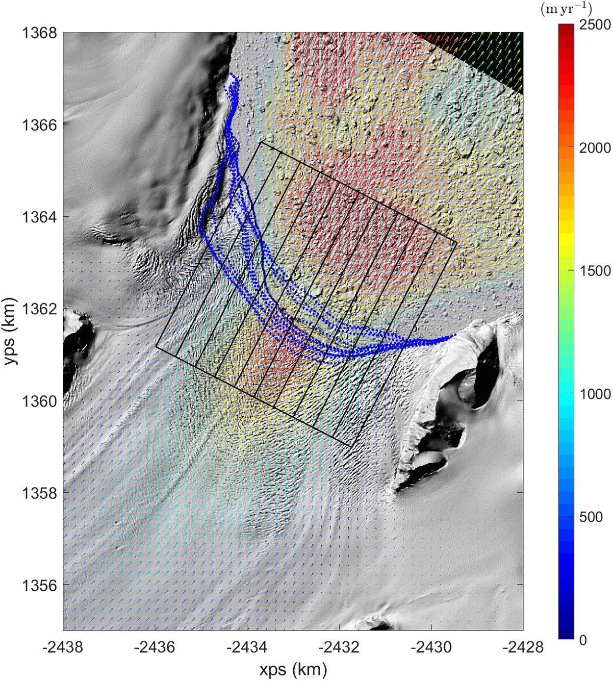
Figure 3. An example of the spatial averaging method, shown at Drygalski Glacier. The base image is a hill shade obtained from the Reference Elevation Model for Antarctica digital elevation model strips (Howat and others, Reference Howat2022a), dated 27 March 2015. A rectilinear box was drawn over the width of the glacier where velocity data spanned the terminus and was aligned with the direction of ice flow. The box was then split into equally spaced segments (solid black lines). The length of each box segment covered the maximum variation in terminus coordinates digitised from each of the digital elevation models (dashed blue lines). Velocity vectors corresponding to the mean velocities over 2015 are plotted for reference (ENVEO and others, Reference Wuite, Hetzenecker, Nagler and Scheiblauer2021).
To calculate the change in terminus position over time, we first calculated the area covered by the glacier in each box segment, i.e. the area in the box covered by the upstream segment boundary to the terminus. The width-averaged change in position between sequential digital elevation models was calculated by dividing the change in area of glacier coverage by the width of the box segment. Similar approaches to assessing spatially averaged terminus position changes have been used in numerous studies (e.g. Moon and Joughin, Reference Moon and Joughin2008; Howat and Eddy, Reference Howat and Eddy2011).
Coordinates were defined at regularly spaced 10 m intervals along each digitised terminus. Starting from the date of the first digital elevation model, monthly average velocity maps were linearly interpolated onto these coordinates up to the date of the next sequential digital elevation model. The velocity maps were projected to the direction normal to the terminus and the mean velocity at each terminus coordinate between sequential digital elevation models was calculated. In turn, the mean coordinate velocities were averaged over each box segment, resulting in a box-average velocity between the dates of sequential digital elevation models. Comparing this to the width-averaged change in terminus position over time, the calving rate in each box segment was determined using Eqn (3).
The cliff height was also assessed at each terminus coordinate. We took the mean surface elevation over a distance 100 m upstream and in the direction normal to the terminus. This process ensured that the extracted heights were not influenced by crevasses or local damage at the ice front and additionally to negate any positional error associated with the digitisation of the terminus location (e.g. Moon and Joughin, Reference Moon and Joughin2008; Hill and others, Reference Hill, Carr and Stokes2017). As per the approach taken to assessing flow velocities, the cliff heights associated with each terminus coordinate were averaged over the width of each box segment to leave a box-average cliff height. Cliff heights and calving rates corresponding to each box segment were compared considering a moving average over a 3 year period and weighted by the durations between each sequential digital elevation model.
The variables used in the averaging processes described above were chosen pragmatically and we anticipated that these may influence the results to some degree. Considering a reference case as described by the variables above, to ensure the employed methodology was robust, we tested the sensitivity of the results to the number of equally spaced box segments (5, 10, 15, 20), resolution of coordinate spacing along the terminus (5 m, 10 m, 20 m, 50 m, 100 m) and time period of the moving window (1 year, 3 years).
5. Results
A correlation between sub-aerial cliff height and calving rate exists, with calving rates seen to increase with greater elevations at the ice front (Fig. 4). A maximum box-average terminus cliff height of 73.1 m was seen at Comrie glacier and corresponded to a box-average calving rate of 2154 m a−1 over the same 3 year window. The maximum observed calving rate was 2456 m a−1 which was seen at Drygalski glacier alongside an average cliff height of 51.4 m.
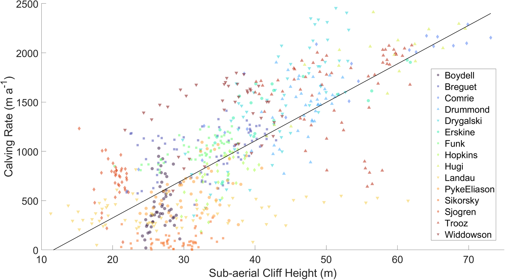
Figure 4. Calving rate is plotted against sub-aerial cliff height for 15 tidewater glaciers around the Antarctic Peninsula. Each data point corresponds to the 3 year moving average values for each single box segment across all glaciers. The solid black line shows the best linear fit (Eqn (4)) with r 2 = 0.529 and root-mean-square error = 419 m a−1.
We derived a calving parameterisation based on the terminus sub-aerial cliff height Hc, considering a linear fit to the collated data (Fig. 4). Using this parameterisation, calving rate c is predicted for all cliff heights as
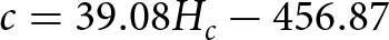 \begin{equation}
c = 39.08H_c - 456.87 \\
\end{equation}
\begin{equation}
c = 39.08H_c - 456.87 \\
\end{equation} for  $H_c \gt 456.87/39.08=11.69\,\mathrm{m}$ and $H_c=0$ otherwise, where Hc is measured in metres and the calving rate, c, in metres per annum.
When glaciers are assessed individually, the relationship between calving rate and sub-aerial cliff height generally holds; however, a number of glaciers do not follow this trend line (Fig. 4). Landau glacier displayed relatively low average calving rates throughout the assessed time period with no increase corresponding to cliff height. Calving rates were observed at close to 500 m a−1 over the entire range of observed box-averaged cliff heights at Landau, which ranged from 11.3 m to 61.5 m. Sikorsky also showed little variation in calving rate ( $ \lt 350\,\mathrm{m\, a^{-1}}$) though the corresponding observed box-averaged cliff heights also covered a small range (21.2–35.5 m). Conversely, Sjögren and Boydell differed from the trendline by displaying a wide variation in calving rates despite cliff heights remaining within a small range (Fig. 4).
As the spatial and temporal averaging processes may impact the observed correlation between cliff height and calving rate, we tested the sensitivity of the results to changing (1) the number of box segments that the glaciers are divided into; (2) the resolution at which the terminus is sampled; and (3) the time period over which the results are averaged.
We found that the correlation between increasing sub-aerial cliff height and calving rate is robust and not sensitive to methods applied in processing the datasets (Fig. 5). The number of segments that the glacier width was divided into had little impact upon the results. Small changes to the gradient of the linear best fit line were observed and r 2 and root-mean-square error (RMSE) values ranged between 0.499–0.594 and 386.2–419 m a−1, respectively (Fig. 5a). Considering the terminus sample resolution, the sensitivities again showed little impact upon the derived best fit line; however, increased scatter was observed at 50 m and 100 m resolutions. At 50 m and 100 m resolution, r 2 values reduced to 0.351 and 0.242, and RMSE values increased to 530 and 673 m a−1, respectively (Fig. 5b). A shallower gradient in the best fit line was derived from the yearly averaged results (Fig. 5c) with higher scatter compared to the reference case (r 2 = 0.392, RMSE = 523 m a−1).
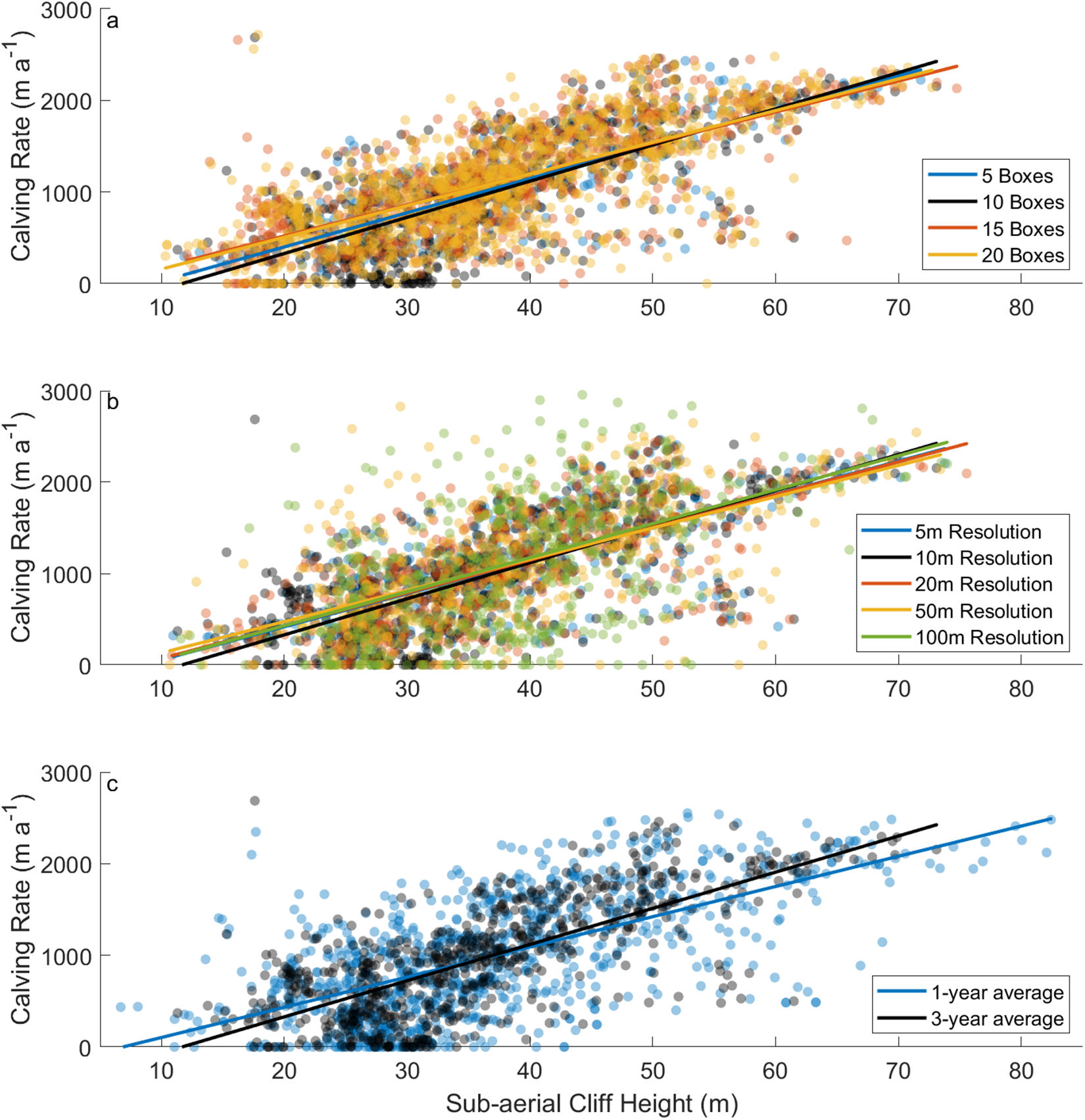
Figure 5. Sensitivity of results to the parameters considered in spatial and temporal averaging. Each colour corresponds to a single sensitivity case encompassing all 15 glaciers. The reference case is given in black and the solid lines represent lines of best fit. (a) Spatial averaging—sensitivity to the number of boxes that the width of each glacier was divided into. (b) Spatial averaging—sensitivity to the resolution at which the terminus was sampled. (c) Temporal averaging–sub-aerial cliff heights and calving rates were assessed considering a yearly average and a 3 year moving window.
6. Discussion
The comparison between observed sub-aerial cliff height and calving rate (Fig. 4) considers (1) spatial differences at each glacier by separating the width of the termini into different boxes and (2) temporal changes by considering the same regions of the termini at different points in time. This results in an overall time-averaged correlation which accounts for geometric and dynamic variation across a glacier’s terminus. Despite this, outliers are seen at Landau, Sjögren, Boydell and Sikorsky, which each display slow flow speeds and thin ice at their fronts (Table 1). In addition, Sikorsky may be considered an exception in terms of terminus width (Table 1) and Landau has relatively few digital elevation models to constrain the relationship between calving rate and cliff height despite a significant difference seen between the maximum and mean cliff heights over the time period assessed.
In contrast to the terminus properties (Table 1), direct measurements are lacking for other factors which may contribute to these outliers. Local geometric features in the bed topography may cause pinning points, modulating the magnitude of terminus stresses and suppressing calving. However, we are unable to confirm whether such locations exist due to uncertainty in present bedrock datasets for the Antarctic Peninsula (Shahateet and others, Reference Shahateet, Navarro, Seehaus, Fürst and Braun2023). Due to these uncertainties, we also assume that the glacier termini are at or close to flotation, which allows us to simplify Eqn (1) leaving an expression showing deviatoric stress being proportional to the sub-aerial cliff height at the terminus (Eqn (2)). Again, without reliable knowledge of the bed topography, it is unclear whether some glaciers are grounded and how the ratio between ice thickness and submerged depth ( $D/H$) may vary between glaciers. Different values of the ratio $D/H$ will impact the calculated deviatoric stress at the terminus compared to when flotation is assumed and, therefore, the same linear relationship between sub-aerial cliff height and calving rate may no longer hold.
Table 1. Details of the studied glaciers, including names, number of high quality digital elevation models (DEMs) available and characteristics of the glacier termini. The reference number corresponds to the numbers labelled in Figure 1 and the dates and time periods covered by the available DEMs are demonstrated in Figure 2
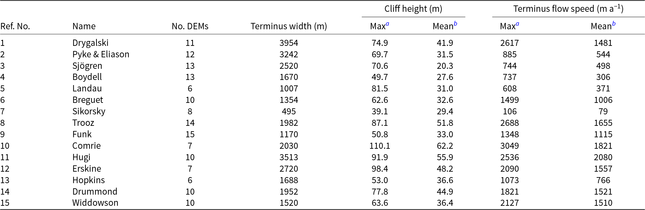
a Maximum single value across all terminus coordinates at any time.
b Mean value across all terminus coordinates and over all time periods.
Given these limitations in knowledge of the terminus geometries, it was important to avoid further reliance upon the understanding of other unknowns. We, therefore, avoided distinguishing between the specific mechanisms driving the observed rates of calving, which is in contrast to the assumptions behind existing calving parameterisations which are based upon the terminus geometry (Mercenier and others, Reference Mercenier, Lüthi and Vieli2018; Schlemm and Levermann, Reference Schlemm and Levermann2019). As we constrain the proportionality between cliff height and calving rate based upon observational data alone, we consider that the long-term calving behaviour of a glacier may be a result of either a single mechanism or a combination of several.
We see similarities to the calving parameterisation presented by Mercenier and others (Reference Mercenier, Lüthi and Vieli2018), in that calving rates are obtained at low cliff heights and increase approximately linearly (Fig. 6). This parameterisation is the only one which we compare to that is derived based upon a tensile failure process, suggesting that the calving behaviours observed in this study may be primarily driven by the same process. The Mercenier and others (Reference Mercenier, Lüthi and Vieli2018) parameterisation overestimates the calving rates which we observed for all cliff heights above 23 m and the derived calving rates diverge with increasing cliff height (Fig. 6). This fundamental difference may be due to the choice of some parameters (such as the fluidity parameter and flow law exponent) in the authors’ idealised case study, which considered a laterally unconfined ice slab lying on a flat bed. As our study is based on observational datasets only, there is no reliance upon assumptions of modelling parameters and our results could, therefore, provide further constraint to any modelling work in this region.
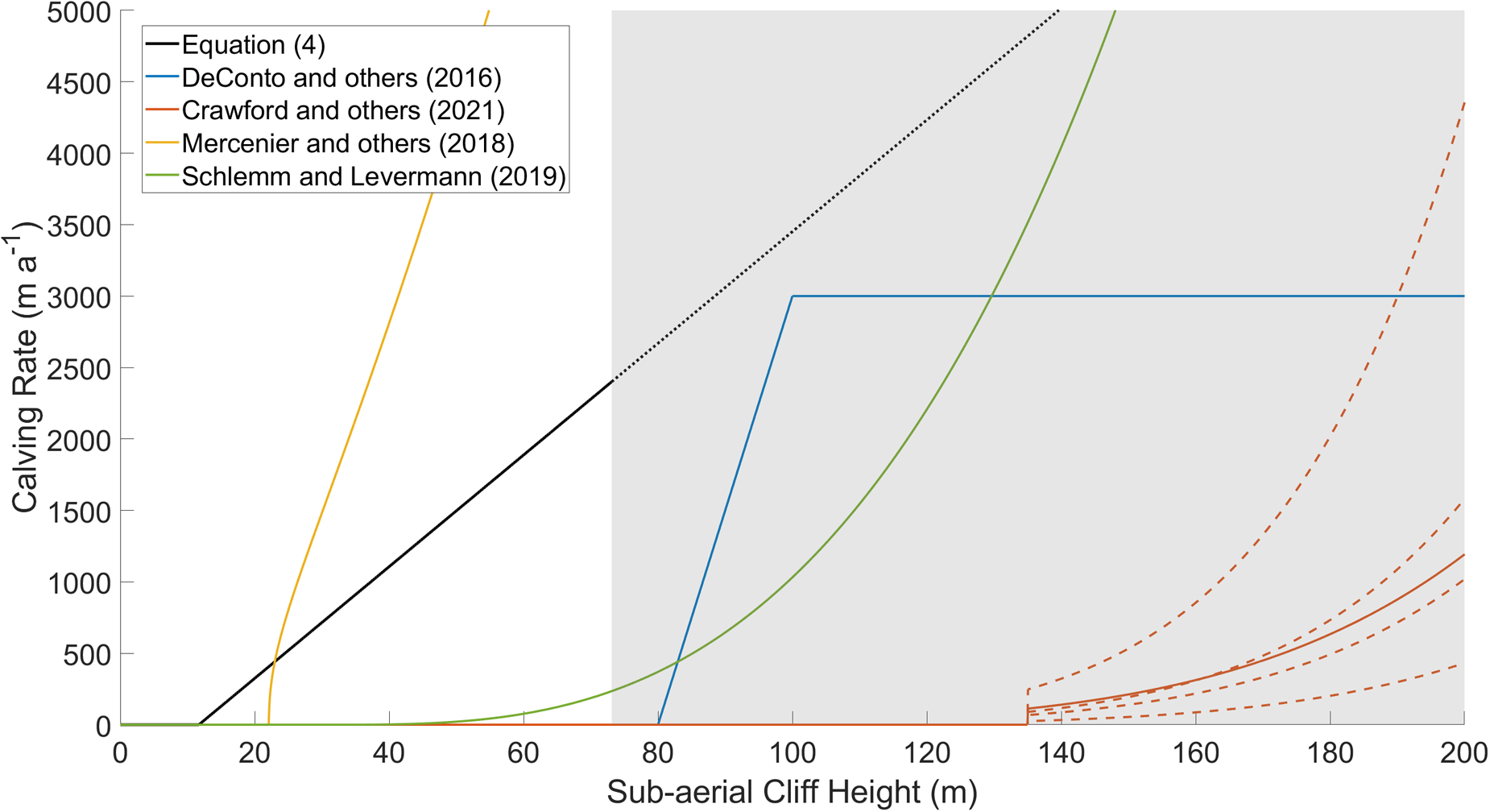
Figure 6. Comparison of parameterisations in which calving rates are dependent upon terminus sub-aerial cliff height. Where submerged depths are required in the parameterisation (Mercenier and others, Reference Mercenier, Lüthi and Vieli2018; Schlemm and Levermann, Reference Schlemm and Levermann2019), the terminus is assumed to be at flotation ( $\frac{D}{H} = 0.89$). The grey box encompasses the area where sub-aerial cliff heights exceed the maximum box-averaged cliff height found in the data analysed in this study and the black dashed line represents where Eqn (4) has been extrapolated over this region. The dashed orange lines show alternative parameterisations due to varying ice temperature and basal slipperiness as described by Crawford and others (Reference Crawford, Benn, Todd, Åström, Bassis and Zwinger2021).
DeConto and Pollard (Reference DeConto and Pollard2016); Crawford and others (Reference Crawford, Benn, Todd, Åström, Bassis and Zwinger2021) and Schlemm and Levermann (Reference Schlemm and Levermann2019) all considered shear failure to be dominant in the derivation of their calving parameterisation. Each of these share the need for a critical cliff height to be reached before calving is predicted. Assuming the terminus is at flotation, Schlemm and Levermann (Reference Schlemm and Levermann2019) required a cliff height of 31 m before the onset of calving. Threshold cliff heights for DeConto and Pollard (Reference DeConto and Pollard2016) and Crawford and others (Reference Crawford, Benn, Todd, Åström, Bassis and Zwinger2021) were 80 m and 136 m, respectively, which both exceed the maximum box-average cliff heights observed in our datasets (Fig. 6). If implemented in an ice-flow model, these parameterisations would all yield calving rates lower than those seen in the observations across large regions of the Antarctic Peninsula leading to unrealistically advancing ice fronts. The accuracy of modelling projections using these parameterisations would, therefore, significantly underestimate mass loss from this region.
Indeed, a notable difference exists between the observed calving rates presented in this study and the rates predicted by all of the existing calving parameterisations (Fig. 6). While Mercenier and others (Reference Mercenier, Lüthi and Vieli2018) calibrated their parameterisation against observational data from a number of tidewater glaciers in the Arctic, the geometric and velocity data that the authors assessed were limited to point data along the calving fronts and at a few snapshots in time. Wider spatial and temporal analysis of the terminus properties may have impacted the observed relationship and altered the calibration. Despite this, the expectation was that their calving parameterisation would be valid globally for any tidewater glacier (Mercenier and others, Reference Mercenier, Lüthi and Vieli2018), though this does not hold for the data assessed around the Antarctic Peninsula.
For the other parameterisations presented in Figure 6, no direct comparison of ice geometry, flow velocity or retreat rate is made against observations. Accurately representing calving in ice-flow models is essential in order to allow for reproduction of realistic glacier dynamics and reliable estimates of ice mass loss, in particular as calving has the potential to induce regimes of unstable retreat that could rise global mean sea level by >1 m within the century (DeConto and Pollard, Reference DeConto and Pollard2016; Lee and others, Reference Lee2023). With the necessary data for assessing observed calving rates now available in high resolution (Howat and others, Reference Howat, Porter, Smith, Noh and Morin2019, Reference Howat2022a), the methodology presented in this study can be used to assess the accuracy with which calving parameterisations proposed through theoretical bases may fit observed data, either locally, regionally or on a global scale. The deviation between Eqn (4) and the parameterisations shown in Figure 6 suggest that these parameterisations may not be indicative of the behaviours seen at tidewater glaciers around the Antarctic Peninsula and validation against data from other regions would be important to demonstrate how suitable they may be more generally.
Theoretical bounds on the stability of ice cliffs have been discussed in numerous studies with the onset of shear failure being controlled by the exceedance of either a prescribed yield strength (Bassis and Walker, Reference Bassis and Walker2012; Ultee and Bassis, Reference Ultee and Bassis2016; Bassis and Ultee, Reference Bassis and Ultee2019; Bassis and others, Reference Bassis, Berg, Crawford and Benn2021) or fracture toughness of ice (Clerc and others, Reference Clerc, Minchew and Behn2019; Parizek and others, Reference Parizek2019). The prescribed material properties ultimately determine the rate at which cliffs fail, however, in practice, high uncertainty exists in real-world material properties due to initiation and transport of damaged ice (Borstad and others, Reference Borstad2012; Mobasher and others, Reference Mobasher, Duddu, Bassis and Waisman2016; Lhermitte and others, Reference Lhermitte2020). For the purposes of large-scale modelling, many difficulties exist in attempting to meaningfully capture the variation in ice rheology and damage both within individual glaciers and between regions. By analysing a wide range of data both spatially and temporally, we arrived at an expression for calving rate which does not directly rely upon knowledge of these varying material properties. However, our study is limited by the maximum sub-aerial cliff heights observed in our analysed datasets. While we observed significant calving rates below the theorised threshold cliff heights required for the onset of shear failure (DeConto and Pollard, Reference DeConto and Pollard2016; Crawford and others, Reference Crawford, Benn, Todd, Åström, Bassis and Zwinger2021), we cannot further constrain the upper bound calving rates under this failure process as these exceed the maximum cliff heights found in the assessed observational datasets (73.1 m box-average). Applying the calving parameterisation derived in this study (Eqn (4)) to cliff heights above this value should, therefore, be done with caution.
Within the analysis of observational data, uncertainty exists from several sources. Firstly, the glacier cliff height may be influenced by uncertainty in the digital elevation model, although errors in the vertical plane are expected to be <1 m (Howat and others, Reference Howat, Porter, Smith, Noh and Morin2019). Further, we make the assumption that the assessed calving fronts are fully vertical. An incline at the terminus may affect the stress regime at the calving front (Mercenier and others, Reference Mercenier, Lüthi and Vieli2018); however, it is difficult to assess such slopes from the analysed datasets. As a variety of real-world glaciers have been assessed, it is anticipated that a range of inclines at the calving fronts are inherently accounted for in the data. However, due to the affect that this variation may have on the terminus deviatoric stresses, the terminus slope is a potential source of scatter in the results. Errors also exist within each monthly averaged velocity dataset, as well as the fact that the dates of the digital elevation models from which the terminus locations are extracted do not fully align with the dates of the velocity products. These uncertainties were negated to a certain extent by deriving the calving parameterisation using a 3 year moving average of both cliff height and calving rate, which allowed for a degree of smoothing in the data compared to averaging over a shorter timescale (Fig. 5c). Validation of the calving parameterisation (Eqn (4)) in a numerical ice-sheet model is required in order to determine its suitability in a modelling application, and whether an adjustment to the parameterisation is needed to make up for data uncertainties.
In addition to uncertainties within datasets, it is noted that the relationship between cliff height and calving rate presented here is derived over a relatively short time period (2015–23). These temporal constraints are due to the first availability of the high-resolution digital elevation models used to constrain the height of the terminus ice cliffs. Variability of ice dynamics over longer timescales (Hanna and others, Reference Hanna2024) may, therefore, not be captured by this calving parameterisation and its applicability to past and future climates is uncertain.
Finally, the calving parameterisation derived in this study (Eqn (4)) is based upon a dataset limited to tidewater glaciers around the Antarctic Peninsula. Further work is required in order to determine the applicability of this parameterisation to tidewater glaciers in different regions, as well as to varying geometries of ice shelves around Antarctica.
7. Conclusion
Through analysis of high-resolution data at 15 tidewater glaciers around the Antarctic Peninsula, a linear relationship between terminus sub-aerial cliff height and calving rate was found. The sub-aerial cliff height is considered a proxy for the near terminus stress regime, with higher stress attributed to increasing calving rates due to multiple driving mechanisms including crevasse propagation and vertical shear.
We showed that existing calving parameterisations which are based upon terminus sub-aerial cliff height offer a poor fit to the observed patterns at these glaciers in the Antarctic Peninsula. With the recent availability of data necessary for high-resolution analysis of both ice geometry and calving rate, better validation and constraint of such calving parameterisations are now possible. An understanding of how well a calving parameterisation fits observational data vastly improves the confidence with which calving can be implemented in modelling applications, in particular if modelling is focussed on a specific region.
The calving parameterisation presented in this study is intended to describe the time-averaged calving response of the tidewater glaciers in the assessed region over long periods, as opposed to capturing individual and specific calving events. Further work is required to validate this parameterisation within a numerical modelling framework and to assess whether such a relationship between calving rate and sub-aerial cliff height exists in other regions.
Acknowledgements
Richard Parsons is supported by the Natural Environment Research Council (NERC) funded ONE Planet Doctoral Training Partnership, NE/S007512/1, hosted by Northumbria and Newcastle Universities. Sainan Sun is funded by grant ISOTIPIC: NERC highlight topics 2023, NE/Z503344/1. G. Hilmar Gudmundsson was partially funded by the Novo Nordisk Foundation, through grant PRECISE, Grant Number NNF23OC0081251 in the call Challenge Programme 2023—Prediction of Climate Change and Effect of Mitigating Solutions.
We acknowledge the use of datasets produced through the ESA project Antarctic Ice Sheet Climate Change Initiative (AIS CCI).
Competing interests
The authors declare that they have no conflict of interest.


 Open access