

Introduction
The presence and properties of organic matter (OM) influence nutrient availability, metal solubilization and carbon biogeochemistry in aquatic ecosystems (Reference Findlay and SinsabaughFindlay and Sinsabaugh, 2003; Reference Mulholland, Findlay and SinsabaughMulholland, 2003; Reference BanaitisBanaitis and others, 2006). The distinction has been made between two important forms of OM: particulate organic matter (POM) and dissolved organic matter (DOM). DOM is defined operationally as OM that passes through filters 0.2–0.8 μm in size (Reference CobleCoble, 2007). DOM typically comprises the largest OM fraction in aquatic systems and is generally considered to be more ecologically significant than POM (Reference Findlay and SinsabaughFindlay and Sinsabaugh, 2003).
The characteristics and ecological functions of DOM in temperate aquatic environments have been studied extensively (e.g. Reference CobleCoble, 1996; Reference Stedmon, Markager and BroStedmon and others, 2003; Reference Holbrook, Yen and GrizzardHolbrook and others, 2006; Reference Yamashita, Jaffé, Maie and TanoueYamashita and others, 2008). However, the role of DOM in glacial environments remains largely unknown, despite evidence that glaciers export DOM and a significant component of this DOM is potentially labile (Reference Lafreniére and SharpLafrenie`re and Sharp, 2004; Reference Barker, Sharp, Fitzsimons and TurnerBarker and others, 2006, Reference Barker, Sharp and Turner2009; Reference HoodHood and others, 2009). As glacier melt rates increase in response to climate warming, so too will the export of glacially derived DOM, and the effects of this DOM on downstream environments may become increasingly important ecologically. Therefore, there is a need to understand the forms and transformations of DOM in glacier systems as these will exert a first-order effect on DOM function in downstream ecosystems.
Organic matter and glacier systems
Glaciers incorporate OM from both allochthonous and autochthonous sources. As glaciers advance over OM in proglacial vegetation and soils (Reference Wadham, Tranter, Tulaczyk and SharpWadham and others, 2008; Reference Barker, Sharp and TurnerBarker and others, 2009), allochthonous OM can be incorporated into basal ice and/or sequestered in the subglacial environment. Allochthonous OM may also be supplied by precipitation, supraglacial streamflow or aeolian transport. Supraglacially deposited OM can be incorporated into glacier ice during the firnification of snow or by transport along englacial hydrological pathways. OM may be incorporated into basal ice from freezing of subglacial meltwaters that are produced by melting at the glacier bed, from waters that are routed from the glacier surface, or through the incorporation of extraglacial sediments and waters during basal ice formation. Autochthonous OM is produced by heterotrophic and/or autotrophic microbial activity. Viable microbial communities have been found in subglacial (e.g. Reference Sharp, Parkes, Cragg, Fairchild, Lamb and TranterSharp and others, 1999; Reference Skidmore, Foght and SharpSkidmore and others, 2000, Reference Skidmore, Anderson, Sharp, Foght and Lanoil2005; Reference FoghtFoght and others, 2004; Reference Bhatia, Sharp and FoghtBhatia and others, 2006), englacial (Reference PricePrice, 2000; Reference Priscu, Christner, Foreman, Royston-Bishop and EliasPriscu and others, 2006) and supraglacial (e.g. Reference Bhatia, Sharp and FoghtBhatia and others, 2006; Reference Stibal, Šabacká and KaštovskáStibal and others, 2006) environments. Evidence indicating that glacial microbial communities are active (Reference Wadham, Bottrell, Tranter and RaiswellWadham and others, 2004; Reference Skidmore, Anderson, Sharp, Foght and LanoilSkidmore and others, 2005) suggests that they may play an important role in DOM cycling through the production and consumption of DOM in glacial systems.
Characterizing DOM using spectrofluorescence
Glacier ice and meltwaters contain relatively low concentrations of DOM, typically less than 2 ppm as organic carbon (Reference Lafreniére and SharpLafrenie`re and Sharp, 2004; Reference Barker, Sharp, Fitzsimons and TurnerBarker and others, 2006; Reference Bhatia, Sharp and FoghtBhatia and others, 2006). Thus, large sample volumes are required to isolate sufficient OM for detailed compositional characterization using techniques such as 13C or 1H nuclear magnetic resonance (NMR) spectroscopy, high-performance liquid chromatography (HPLC) and electrospray ionization Fourier transform ion cyclotron resonance mass spectrometry (ESI-FTICR-MS) (e.g. Reference Leenheer and CrouéLeenheer and Croué, 2003; Reference Sleighter and HatcherSleighter and Hatcher, 2008; Reference Bhatia, Das, Longnecker, Charette and KujawinskiBhatia and others, 2010). Total fluorescence spectroscopy is a sensitive technique that requires small sample volume and DOM concentration and little sample preparation, making it well suited to characterizing the fluorescing components of DOM in dilute solutions from a large number of samples.
Several DOM fractions are composed of fluorophores, compounds that absorb and re-emit electromagnetic energy (Reference Mopper, Feng, Bentjen and ChenMopper and others, 1996). Studies of DOM fluorescence have shown that specific fluorophores are associated with the presence of particular compounds in the DOM (e.g. Reference CobleCoble, 1996, Reference Coble2007; Reference Coble, del Castillo and AvrilCoble and others, 1998; Reference LakowiczLakowicz, 1999; Reference Marhaba and LippincottMarhaba and Lippincott, 2000; Reference Marhaba, Van and LippincottMarhaba and others, 2000; Reference Parlanti, Wortz, Geoffroy and LamotteParlanti and others, 2000). These fluorescent signatures do not directly identify the presence of specific compounds, but they do provide evidence for the presence of DOM fractions that can be characterized as, for example, humic-like, fulvic-like, tryptophan-like or tyrosine-like (Reference Hudson, Baker and ReynoldsHudson and others, 2007). Here, mixtures of tryptophan-and/or tyrosine-like DOM are referred to as proteinaceous.
The total spectrofluorescence of DOM in a sample is represented by an excitation–emission matrix (EEM). EEMs comprise a series of fluorescence scans that measure light emitted over a range of wavelengths as the result of excitation at series known wavelengths, yielding a ‘map’ of fluorophore intensity (Reference Coble, Green, Blough and GagosianCoble and others, 1990). Fluorophores in DOM can be identified by the location and shape of their peak fluorescence intensity in the EEM and can be compared between samples. Total spectrofluorescence has the advantage of describing fluorescence over a broad range of wavelengths and is thus more suitable than other spectrofluorescent techniques for analyzing DOM that contains multiple fluorophores.
Parallel factor analysis (PARAFAC)
EEMs have often been interpreted visually by noting the emission and excitation coordinates of fluorophore peak intensities (e.g. Reference CobleCoble, 1996). For example, tyrosine-like fluorescence has a peak at wavelengths of 275 nm excitation and 310 nm emission (Reference CobleCoble, 1996). However, fluorophores cannot always be distinguished satisfactorily using visual analysis as individual peaks may overlap or be poorly resolved (Reference BroBro, 1997). Owing to the inherent complexity of spectral signatures arising from a complex mixture of DOM fractions in natural waters, parallel factor analysis (PARAFAC) provides a less subjective way to interpret a complex EEM (Reference Stedmon, Markager and BroStedmon and others, 2003). PARAFAC reduces the dimensions of a dataset and allows for the identification of a small number of prominent fluorophores.
PARAFAC is designed for the analysis of data arrays with more than two dimensions (Reference Rutledge and BouveresseRutledge and Bouveresse, 2007). When applied to EEMs, PARAFAC decomposes three-dimensional spectral signatures that may involve multiple overlapping fluorophores into loadings associated with individual components that can be related to specific DOM fractions (Reference BroBro, 1997; Reference Andersen and BroAndersen and Bro 2003; Reference Smilde, Bro and GeladiSmilde and others, 2004). PARAFAC yields a model that represents a unique solution obtained by a least-squares fit to observations that minimizes residuals (Reference BroBro, 1999; Reference Ohno and BroOhno and Bro, 2006). This model may then be applied to the interpretation of the original array of EEMs. Reference Andersen and BroAndersen and Bro (2003) provide comprehensive descriptions of the development of PARAFAC.
Methods
Field sites
Eighty ice and meltwater samples were analyzed for their fluorescence properties. Samples were obtained from: Clark Glacier (CG), Suess Glacier (SG), Victoria Upper Glacier (VUG) and Lower Wright Glacier (LWG), McMurdo Dry Valleys, Antarctica; John Evans Glacier (JEG) and Prince of Wales Icefield (PoW), Ellesmere Island, Canada; and Engabreen (EG) in the Norwegian Arctic (Table 1).
Table 1. Glacier systems and samples

The Antarctic glaciers are cold throughout (cold-based polar glaciers), with ice temperatures below the pressure-melting point. Proglacial lakes, which may be a source of lacustrine OM, are found in front of SG, VUG and LWG. There were several large proglacial lakes in the McMurdo Dry Valleys during the Last Glacial Maximum (LGM) and early Holocene (Reference Hall, Denton and OverturfHall and others, 2001). Any of the glaciers sampled may have advanced over lacustrine sediments and incorporated associated OM into their basal ice layers, either as POM in sediment or DOM in basal ice formed by freezing of lake water and/or sediment pore water to the glacier sole (Reference Souchez and JouzelSouchez and Jouzel, 1984). CG contains a considerable amount of englacial and surficial wind-blown dust, suggesting a possible aeolian OM input derived from exposed proglacial lake sediments, embryonic soils and/or the nearby marine system of McMurdo Sound. Aeolian transport of marine-derived OM may also be an important OM source to LWG, which, of the Dry Valley glaciers sampled, is the closest to McMurdo Sound.
JEG and PoW are located on eastern Ellesmere Island, Canada, in tundra characterized by sparse High Arctic vegetation. JEG is a polythermal glacier that has overrun OM in vegetation and soils and has incorporated OM into its basal ice (Reference WillerslevWilleslev and others, 2007). PoW is located near Nares Strait and the North Open Water polynya, and wind-deposited marine-derived OM may be a locally important OM source.
EG, in the Norwegian Arctic, is located within 3 km of a fjord and 30 km of the open Atlantic Ocean, suggesting that marine aerosols may be a potentially important source of OM. Furthermore, EG is situated near a birch forest, and terrestrially derived OM is deposited onto the glacier surface, transported through the glacier along hydrological pathways to the subglacial environment and likely incorporated into basal ice by refreezing of subglacial water.
Sampling methods and sample descriptions
Table 2 describes the samples analyzed in this study. We collected all ice samples (except JEG ice-core samples and EG basal ice samples) using an ethanol-bathed flame-sterilized chisel and aluminium collection tray. JEG ice-core samples were collected using a Kovacs ice-coring drill. EG basal ice samples were collected by inserting a pre-combusted (450°C for 8hours) ice screw into the basal ice exposed in the walls of an ice cave created with a hot-water drill from within the Svartisen Subglacial Laboratory. All ice samples were stored frozen in either sterile Whirlpak bags or sterile McCartney vials.
Table 2. Sample descriptions
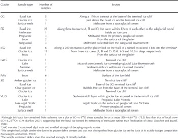
Meltwater samples were collected in acid-washed (HCl) and pre-combusted (450°C for 8hours) 250mL amber or universal glass bottles. Each bottle was rinsed three times with filtered sample before the analytical sample was collected and frozen for storage. EG meltwater samples were filtered in the field using a manual vacuum pump and 0.7 μm glass-fibre (GF/F) filter papers and were stored frozen in McCartney vials.
Spectrofluorescence analysis
The 80 samples were kept frozen from the time of collection (Table 1) until sample preparation in March–June 2008. Subsamples from the JEG ice cores were cut using a bandsaw and the ice surfaces were subsequently scraped with an ethanol-cleaned microtome blade to remove possible contamination. All samples were handled with sterile gloves and stored and melted in the dark at room temperature in sterile Whirlpak sample bags. All melted samples were filtered and stored as described above.
Each sample was filtered through pre-combusted (450°C for 8 hours) 0.7 μm glass-fibre (GF/F) filter papers using an acid-washed and pre-combusted (450°C for 8 hours) glass filtration system. The upper chamber of the filtration system was rinsed three times with sample. An aliquot was then filtered to rinse the lower chamber of the system three times before the remaining volume was filtered as sample for analysis. The sample was transferred to a 40 mL acid-washed and pre-combusted (450°C for 8 hours) amber glass vial. Vials were stored in the dark at ∼4°C for up to 3 weeks prior to analysis, except for the EG samples which were frozen immediately after sampling and then melted and filtered directly prior to analysis. Although the effects of freeze/thaw processes on fluorescent characteristics are not well understood, large and variable responses have been observed due to freeze/thaw cycles (Reference Spencer, Bolton and BakerSpencer and others, 2007).
Replicates of a melted JEG ice-core sample were analyzed four times at 2 week intervals to determine the effect of storage on sample spectrofluorescence. Results indicate that although the peak locations did not change, the maximum fluorescent intensities of the humic- and proteinlike components differed by up to 20% between the replicates. However, the relative proportions of proteinaceous and humic DOM fluorescence remained constant; humic and proteinaceous fractions deviated <2% between the replicate samples, whereas the standard deviation in humicprotein fluorescence ratio was 10% for the remainder of the dataset. This suggests that comparisons between total proteinaceous and humic-like DOM fluorescence remain valid. No additional replicates were taken due to the limited sample sizes available.
Filtered samples were warmed to 21°C in a water bath for 1–2 hours prior to analysis with a Fluorolog-3 spectro-fluorometer equipped with a xenon lamp as excitation source. For analysis, samples were placed in a quartz glass cuvette, with a 10 mm path length, that had been rinsed three times with deionized (DI) water and three times with sample. Fluorescence scanning was performed with internal and dark correction applied. The Raman intensity of the instrument was measured using DI water at the beginning of each analysis day, with excitation set to 350 nm, and emission intensities were measured at 2 nm increments from 365 to 450 nm. The lamp intensity did not fluctuate more than 10% over the course of the analyses. EEMs were created for all samples by scanning at 2 nm emission wavelength increments from 300 to 550 nm and 5 nm excitation wavelength increments from 250 to 450 nm using an integration time of 0.5 s and 10nm slits. DI water was also scanned each day.
PARAFAC
EEMs were Raman-corrected by subtracting the daily EEM for DI water. Data from the high-intensity area of each EEM attributable to the Rayleigh-Tyndall effect were removed (Reference Andersen and BroAndersen and Bro, 2003; Reference Ohno and BroOhno and Bro, 2006). As fluorescent molecules always emit energy at wavelengths longer than that at which they are excited, fluorescent peaks cannot occur in areas of the spectrum in which emission wavelengths are smaller than corresponding excitation wavelengths. Data from this part of each spectrum were therefore removed (Reference Andersen and BroAndersen and Bro, 2003).
PARAFAC was performed in Matlab 7.6.0 using the DOMFluor toolbox (http://www.models.life.ku.dk) which contains the N-Way toolbox v.3.1 created by Reference Andersson and BroAndersson and Bro (2000). Code and procedures used in this study followed Reference Stedmon and BroStedmon and Bro (2008).
The fluorescent intensity (FI) of a DOM component is proportional to its concentration in a sample (e.g. Reference Parlanti, Wortz, Geoffroy and LamotteParlanti and others, 2000; Reference Christensen, Miquel Becker and FrederiksenChristensen and others, 2005; Reference LucianiLuciani and others, 2008; Reference Airado-Rodrıguez, Galeano-Díaz, Durán-Merás and WoldAirado-Rodríguez and others, 2009). FI varied by up to two orders of magnitude between samples. The samples with highest FI influenced the PARAFAC model dramatically as they accounted for a considerable proportion of the variance in the dataset. To minimize variation due to FI and to maximize the number of samples remaining in the modeled data, all EEMs were standardized to their maximum FI. This effectively reduces the inter-sample variability in FI and allows the analysis to focus on EEM composition. Each sample can be interpreted according to the percentage contribution of each fluorescent component to the total fluorescence of its spectrum. PARAFAC models with up to 15 components were created. Outliers with leverages >0.5 were removed from the dataset (Reference Stedmon and BroStedmon and Bro, 2008).
Model validation
Of the 15 PARAFAC models, the model with the most appropriate number of components was determined using the following criteria:
Sum of squared error: Relatively large reductions in the sum of squared error between two models favoured the model with the greater number of components, whereas relatively small reductions in the sum of squared error favoured the model with fewer components (Reference Stedmon and BroStedmon and Bro, 2008). In all cases, models with relatively low sum of squared error were selected.
EEM residuals: After an appropriate model has been fitted to all EEMs, only random noise should remain in the residual spectra. However, this noise may also include weakly fluorescing components that are difficult to distinguish from instrument noise, quenching effects, remnant inner filter effects and scattering effects (Reference Stedmon and BroStedmon and others, 2003). Residuals were inspected to ensure that the maximum possible number of discernible fluorophores was modeled correctly.
Visual inspection of the modeled components: (1) Modeled fluorescent emission peaks should have a near-Gaussian distribution (Reference Stedmon, Markager and BroStedmon and others, 2003; Reference Kowalczuk, Stoé-Egiert, Cooper, Whitehead and DurakoKowalczuk and others, 2005), although broad or multiple excitation peaks may exist due to electrons being excited to various vibrational sublevels (Reference Stedmon, Markager and BroStedmon and others, 2003). (2) Since 10 nm slits were used for spectrofluorescence scanning, components with peaks <10nm apart were considered not to be significantly different. (3) It was assumed that each component modeled only one group of fluorophores and that components with multiple emission peaks were poorly modeled (Reference Stedmon, Markager and BroStedmon and others, 2003). (4) Since data in the area of Rayleigh scatter were removed, component peaks in this region of an EEM were considered to be erroneous.
The validity of a PARAFAC model to describe variance in a dataset accurately is often evaluated using split-half analysis (Reference Harshman, Lundy, Law, Snyder and McDonaldHarshman and Lundy, 1984). However, split-half analysis is unlikely to validate a model if the dataset is too small relative to the intra-sample variance (Reference Stedmon and BroStedmon and Bro, 2008). Because the samples in this dataset are from geographically diverse locations and different sub-environments which are unlikely to be well mixed, fluorescence is expected to be highly variable. None of the models explored in this study satisfied the split-half analysis and thus it could not be used as a validation tool.
Model interpretation
The maximum relative FI (RFI) value was extracted for each component in each EEM. Although RFI values are a function of fluorophore concentration, two other factors also contribute. First, the Beer–Lambert law indicates that the intensity of light emitted upon excitation of a fluorophore is dependent on its absorption coefficient. Absorption coefficients vary with molecular characteristics and will thus differ between fluorophores. Secondly, each sample was standardized to its maximum FI, so component concentrations in different samples are not equally proportional to RFI. These two factors do not influence the relative contributions of each component to the overall fluorescence in an EEM. Thus, cluster analysis was performed on the relative intensities of protein-like (components 1 , 2, 4 and 5) and humic-like (component 3) fluorophores in each EEM. Cluster analysis arranges a dataset into like-groups while minimizing within-group variability. The analysis was preformed in Statistica Version 8 using Euclidean distances and complete linkages. An agglomeration dendrogram plot was used to identify similarities and differences between samples, glacier systems and glacier environments.
Results and Discussion
Five-component PARAFAC model
A five-component PARAFAC model (Fig. 1 ; Table 2) optimized the evaluation criteria outlined above and explained 98.2% of the variance in the dataset. We stress that a five-component model does not necessarily mean that the EEMs produced in this study contained only five fluorophores. The extraction of five components simply indicates that these components accounted for significant fractions of the variance in the dataset. Other fluorophores may not have been modeled because they had weak fluorescence, because their spectra were similar to those of other fluorophores or because they occurred in relatively few samples (Reference Stedmon, Markager and BroStedmon and others, 2003). Visual inspection of the residuals from the model EEM can be used to identify the presence of additional fluorophores. If a model describes all discernible fluorophores in an EEM correctly, only noise will remain as residual. In this study, 31 of the 69 modeled EEMs had fluorescence residual patterns containing identifiable peaks. This suggests the presence of additional fluorophore groups at wavelengths shown in Figure 2. Most of these lie in the region of ‘soluble microbial by-productlike fluorophores’ (Reference Chen, Westerhoff, Leenheer and BookshChen and others, 2003).

Fig. 1. EEMs for the five-component PARAFAC model.

Fig. 2. Bubble plot of residual component. Bubbles are centered over visually identified residual peaks. The size of the bubbles represents the frequency at which the particular peak was observed to occur in the residuals. The peak represented by the smallest bubble has a frequency of 1, while the peak represented by the largest bubble has a frequency of 11. Regions of humic acid-like and soluble microbial by-product-like (Reference Chen, Westerhoff, Leenheer and BookshChen and others, 2003) are included.
Although the five-component model was not validated by split-half analysis and contained residuals that suggest the presence of additional fluorophores, these represented <1.8% of the variance in the dataset. The concern with interpreting data from an unvalidated PARAFAC model lies in the possibility that one or more of the components reflect noise rather than true fluorophore signals. This is unlikely to be the case with the five-component model presented here because it excluded recurring peaks in the residual EEMs (Fig. 2), suggesting the presence of additional fluorophores of considerably higher intensity than background noise.
Component descriptions
The fluorescent loading patterns of the five modeled components (Table 3; Fig. 1) can be matched to fluorophores described in the literature (Table 4). Component 3 has been identified previously as humic-like, while the others have been identified as protein-like.
Table 3. Description of the five-component PARAFAC model. Wavelengths in parentheses represent a secondary peak

Table 4. Relevant common fluorophores identified in previous studies

Component 3 is similar to a humic-like peak A fluorophore (Reference CobleCoble, 1996) described from marine and terrestrial environments (Reference Coble, Green, Blough and GagosianCoble and others, 1990, Reference Coble, del Castillo and Avril1998; Reference De Souza Sierra, Donard, Lamotte, Belin and EwaldDe Souza Sierra and others, 1994; Reference CobleCoble, 1996), including forests and wetlands (Reference Stedmon, Markager and BroStedmon and others, 2003). The relatively long emission wavelengths of this peak suggest more conjugated fluorescent molecules than are found in the other components (Reference Sharma and SchulmanSharma and Schulman, 1999). This component may therefore represent terrestrially derived humic matter of high molecular weight (Reference Stedmon, Markager and BroStedmon and others, 2003) that is less labile than proteinaceous OM.
Component 1 closely resembles the tryrosine-like peak B fluorophore (Reference CobleCoble, 1996) and indicates autochthonous production of DOM (Reference Stedmon and MarkagerStedmon and Markager, 2005b). Component 2 matches the tryptophan-like fluorescent characteristics described by Reference LakowiczLakowicz (1999) and peak T described by Reference CobleCoble (1996). Typically, tryptophan is associated with the autochthonous production of DOM through biological degradation (Reference Mopper and SchultzMopper and Schultz, 1993; Reference Coble, del Castillo and AvrilCoble and others, 1998; Reference Stedmon and MarkagerStedmon and Markager, 2005b; Reference Murphy, Stedmon, Waite and RuizMurphy and others, 2008) and its production has been observed during algal blooms (Reference Stedmon and MarkagerStedmon and Markager, 2005a).
The fluorescent characteristics of component 4 cannot be interpreted directly on the basis of previous studies. The emission maximum at 330 nm lies between those of tryptophan-like and tyrosine-like fluorescence. The excitation maximum at 250nm is at a shorter wavelength than those reported for tyrosine and tryptophan fluorescence by some authors (e.g. Reference CobleCoble, 1996; Reference Stedmon, Markager and BroStedmon and others, 2003; Reference Stedmon and MarkagerStedmon and Markager, 2005a; Reference Yamashita, Jaffé, Maie and TanoueYamashita and others, 2008), but at a longer wavelength than reported by other authors (e.g. Reference Marhaba and LippincottMarhaba and Lipincott, 2000; Reference Marhaba, Van and LippincottMarhaba and others, 2000; Reference Parlanti, Wortz, Geoffroy and LamotteParlanti and others, 2000). The emission maximum lies between those of tyrosine and tryptophan. This may be a consequence of a shifted peak, which could be attributable to: (1) formation in a different microenvironment resulting in difference in amino acid composition (Reference Determann, Lobbes, Reuter and RullkötterDetermann and others, 1998); (2) differences in concentration that influence inner filtering effects and excitation/ emission wavelengths (e.g. Reference Mobed, Hemmingsen, Autry and McGownMobed and others, 1996; Reference Hautala, Peuravuori and PihlajaHautala and others, 2000); or (3) different solution properties such as pH and salinity (Reference Stedmon, Markager and BroStedmon and others, 2003). Several other studies have also reported red or blue shifted protein peaks (e.g. Reference Maie, Scully, Pisani and JafféMaie and others, 2007; Reference Yamashita, Jaffé, Maie and TanoueYamashita and others, 2008).
The primary peak in component 5 is located between peaks T and B of Reference CobleCoble (1996). As both tryptophan and tyrosine are associated with amino acids in proteins, this component can be interpreted more broadly as protein-like. Component 5 has a secondary emission peak at 400 nm that is similar to the humic-like fluorescence of peaks A and C (Reference CobleCoble, 1996). As the intensity of this peak is considerably smaller than the protein-like peak, component 5 is considered to be primarily protein-like.
Microbial source of DOM in glacier systems
The four protein-like components accounted for 89% of the modeled fluorescence while the humic-like component (3) accounted for the remaining 11%. Over 70% of the total modeled fluorescence in all samples is proteinaceous. This does not mean, for example, that 89% of the DOM in the dataset is proteinaceous, since each fluorophore group emits energy at different intensities according to the Beer–Lambert law. However, the proteinaceous nature of four of the five modeled components and its potentially microbial origin (e.g. Reference Mopper and SchultzMopper and Schultz, 1993; Reference Coble, del Castillo and AvrilCoble and others, 1998; Reference Stedmon and MarkagerStedmon and Markager, 2005a,Reference Stedmon and Markagerb) suggests a significant microbial source of DOM in these cold environments. Likewise, Reference Barker, Sharp, Fitzsimons and TurnerBarker and others (2006) concluded that DOM in glacier ice is predominantly ‘microbial’ in character and Reference Lafreniére and SharpLafreniére and Sharp (2004) found that DOM in glacier runoff was more ‘microbial’ than the more ‘terrestrial’ DOM in nearby snowmelt-fed streams. From a study of 11 Alaskan watersheds, Reference HoodHood and others (2009) found that watersheds with high glacier cover have a higher proportion of proteinlike fluorescence than those with little or no glacier cover. This contrasts with DOM from marine, estuarine and fluvial environments, in which humic-like fluorescence makes up a more significant fraction (at least half) of the total modeled fluorescence and the predominant component(s) are humic-like (e.g. Reference CobleCoble, 1996; Reference Stedmon, Markager and BroStedmon and others, 2003; Reference Holbrook, Yen and GrizzardHolbrook and others, 2006; Reference Yamashita, Jaffé, Maie and TanoueYamashita and others, 2008).
Transformations of OM are expected to occur throughout the glacial system as environmental conditions (e.g. solar radiation, temperature, and oxygen and water availability) change. For example, in the supraglacial environment, where liquid water, solar radiation and temperatures above 0°C can be present, photoautotrophic microbial processes can occur (Reference Stibal, Tranter, Benning and RehákStibal and others, 2008). Conversely, the englacial environment is characterized by cold temperatures, little to no light and limited water availability. Although viable microorganisms with different physiological characteristics have been identified englacially, it is still unknown whether they are active in situ. OM can be transformed in subglacial environments where liquid water often exists. Owing to the complete darkness and anaerobic conditions at glacier beds, these processes can involve heterotrophic and autotrophic pathways (Reference Skidmore, Foght and SharpSkidmore and others, 2000). Proglacially, where solar radiation, warm air temperatures and water are more abundant, heterotrophic, autotrophic, abiotic humification and photolysis may transform DOM more readily.
Samples did not cluster according to either the glacier system or the geographical region from which they originated, suggesting that there are no significant differences in DOM characteristics between the seven glacier systems studied (Fig. 3). For example, cluster 1 contains samples from all the glacier systems included in this study and from snow, glacier ice and basal ice. The similarities in the properties of DOM from different glaciers and glacial sub-environments and the generally proteinaceous character of DOM suggest the ubiquitous occurrence of a few relatively unique DOM fractions. This may indicate the potentially widespread presence of microbially derived DOM in glaciers. Previous work has shown the subglacial environment to be a viable microbial habitat containing diverse microbial assemblages (Reference Sharp, Parkes, Cragg, Fairchild, Lamb and TranterSharp and others, 1999; Reference Skidmore, Foght and SharpSkidmore and others, 2000; Reference Bhatia, Sharp and FoghtBhatia and others, 2006; Reference LanoilLanoil and others, 2009) that appear to be active (Reference Wadham, Bottrell, Tranter and RaiswellWadham and others, 2004; Reference Skidmore, Anderson, Sharp, Foght and LanoilSkidmore and others, 2005). Microbes have also been identified in englacial environments (Reference PriscuPriscu and others, 1999), and surficial glacier ice and snow contain active and diverse assemblages of bacteria, cyanobacteria and algae (Reference Stibal, Šabacká and KaštovskáStibal and others, 2006; Reference Foreman, Sattler, Mikucki, Porazinska and PriscuForeman and others, 2007; Reference Anesio, Hodson, Fritz, Psenner and SattlerAnesio and others, 2009). Bacteria have also been identified as important snow nucleators (Reference Carpenter, Lin and CaponeCarpenter and others, 2000). A number of heterotrophic and autotrophic processes may occur within the glacial system, such as methanogenesis, sulphate reduction, nitrate reduction, aerobic chemoheterotrophy (Reference Skidmore, Foght and SharpSkidmore and others, 2000) and photosynthesis (Reference Stibal, Šabacká and KaštovskáStibal and others, 2006).

Fig. 3. Cluster analysis using the total protein-like and humic-like RFIs for the modeled EEMs. Euclidean distances and complete linkages were applied.
Environmental occurrences of protein-like and humic-like fluorescence
The dendrogram generated by cluster analysis performed on the RFIs for the humic- and protein-like components of each sample identified four main sample clusters defined at a linkage distance of 3 (Fig. 3). These clusters reflect differences in the relative proportions of protein- and humic-like fluorescence (Fig. 4). Clusters 1 and 2 contain samples with greater protein-like fluorescence (mean: 92.9±2.8%), whereas clusters 3 and 4 contain samples with relatively more humic-like fluorescence (mean: 19.1 ±4.6%; Fig. 4).

Fig. 4. Average percent of total modeled fluorescence for each cluster. Error bars indicate one standard deviation.
Samples from all glacier systems (except CG) are found in all clusters. CG samples have consistently high protein-like fluorescence and are found only in clusters 1 and 2. Samples of snow and glacier ice are found throughout the dendrogram and have similar DOM characteristics, likely because glacier ice is formed from snow. This suggests that both snow and glacier ice acquire OM from atmospheric sources (e.g. snow-nucleating bacteria, wind-blown material) or from microbial production on the glacier surface.
Basal ice samples are also found in all clusters. Basal ice forms by the accretion of ice and debris onto the base of the glacier through processes of regelation and congelation (Reference KnightKnight, 1997). Regelation involves the refreezing of water that originates from localized pressure-induced melting at the glacier bed, while congelation involves the formation of ice at the base of the glacier from water derived primarily from melting at the glacier surface. Although it is possible that basal ice has acquired much of its OM through the recycling of glacier ice, these sub-environments contain very different microbial habitats, chemical environments and OM sources (e.g. Reference Skidmore, Foght and SharpSkidmore and others, 2000; Reference Bhatia, Sharp and FoghtBhatia and others, 2006). The spectrofluorescence analysis has not captured these differences. However, four basal ice samples, from JEG, CG and SG, were identified as outliers from the model and were removed from the dataset (Fig. 5b–e). The unique spectra of these samples were not effectively described by the five-component PARAFAC model, suggesting the presence of unique DOM in the subglacial environment at these glaciers.

Fig. 5. Unmodeled EEMs for the 16 outliers removed during PARAFAC modeling. (a–g) Ice samples; (h–p) water samples.
The modeled meltwater samples are clustered alongside samples from other subglacial, englacial and supraglacial environments (Figs 3 and 4), suggesting that glacier meltwater either inherits DOM characteristics from its source ice and/or has similar OM sources. For example, the three meltwater samples from EG are similar to the majority of basal ice samples from EG and contain a relatively high proportion of humic-like fluorescence (Figs 3 and 4). This confirms the routing of runoff at EG through the subglacial environment (Reference Lappegard, Kohler, Jackson and HagenLappegard and others, 2006). This is especially true of the winter months when the sampling was conducted. At this time, subglacial meltwater is the primary water source to the proglacial stream since there is almost no surface melting. The OM source in this case is likely to be glacially overridden or inwashed soils from the local birch forest.
Although meltwater samples are broadly similar to glacier ice samples, they are significantly over-represented in clusters 3 and 4, while glacier ice samples are significantly over-represented in clusters 1 and 2 (x2 = 14.2, df=7, p<0.05) (Fig. 3). Clusters 3 and 4 have notably higher humic-like:protein-like fluorescence ratios than clusters 1 and 2 (Fig. 4). Furthermore, 9 of the 16 samples removed as outliers with leverages >0.5 during PARAFAC runs were proglacial and supraglacial water samples from CG, LWG, VUG and EG (Fig. 5h–p). These samples also contained primarily humic-like fluorophores (Figs 2 and 5h–p). Possible explanations for the high humic-like:protein-like fluorescence ratios in meltwater samples include the following: (1) meltwater may access humic OM sources as it is routed through the glacier and proglacial environment; (2) labile proteinaceous DOM may be removed from samples by microbial consumption of tryptophan or tyrosine (Reference Parlanti, Wortz, Geoffroy and LamotteParlanti and others, 2000), by abiotic humification or by photolysis of DOM into non-fluorescent forms (Reference Bertilsson, Jones, Findlay and SinsabaughBertilsson and Jones, 2003), which may not occur to the same extent in ice and snow; and (3) aquatic environments may be more favourable than ice environments for the production of humic-like fluorophores, especially if waters have access to supplies of terrestrial nutrients.
Conclusions
PARAFAC was performed on spectrofluorescence data from the subglacial, englacial, supraglacial and proglacial environments of seven glacier systems in the McMurdo Dry Valleys, Antarctica; Ellesmere Island, Canada; and the Norwegian Arctic. DOM from the different glacier systems can be described by five fluorescent components: one humic-like and four protein-like (one tyrosine-like, one tryptophan-like and two undefined).
In contrast to DOM from marine, estuarine and fluvial environments, which is dominated by humic-like material, DOM from glacier systems is dominated by protein-like DOM that may be derived microbially. Other studies have reported similar protein-like DOM from glacial runoff in Alaska (Reference HoodHood and others, 2009), Canada (Reference Lafreniére and SharpLafreniére and Sharp, 2004; Reference Barker, Sharp, Fitzsimons and TurnerBarker and others, 2006, Reference Barker, Sharp and Turner2009) and in ice from an Antarctic glacier (Reference Barker, Sharp, Fitzsimons and TurnerBarker and others, 2006). There were no significant differences in the fluorophores present in DOM from the range of glacier systems studied here, despite differences in geographic location, glacier thermal regime and potential OM sources. Although DOM from ice (basal, englacial and surficial), snow and meltwater samples has remarkably similar characteristics, meltwater samples do have consistently higher humic-like:protein-like fluorescence ratios than snow and ice samples. This suggests that either additional humic DOM is introduced to the meltwater as it is routed through the glacier system or protein-like DOM is removed from meltwater by organic processes, such as heterotrophy (e.g. Reference Fellman, D’Amore, Hood and BooneFellman and others, 2008), or through inorganic process such as abiotic humification (e.g. Reference Parlanti, Wortz, Geoffroy and LamotteParlanti and others, 2000) occurring along the flow route or photolysis (e.g. Reference Miller, McKnight and ChapraMiller and others, 2009).
Acknowledgements
This research was funded by the Natural Sciences and Engineering Research Council of Canada (Discovery and Research Tools and Instruments grants, Undergraduate Summer Research Assistantship), the Canada Foundation for Innovation, Polar Continental Shelf Project, Canadian Circumpolar Institute, Northern Scientific Training Program, Antarctica New Zealand, Environment Canada and the UK Natural Environment Research Council. We thank the Nunavut Research Institute and the communities of Grise Fjord and Resolute Bay for permission to conduct research on Ellesmere Island, the Norwegian Water Resources and Energy Directorate for allowing access to the Svartisen Subglacial Laboratory, and the anonymous reviewers of this paper.


