

Introduction
During the past decade, Arctic sea ice has undergone a significant change, resulting in rapid retreat in ice extent (Reference Comiso, Parkinson, Gersten and StockComiso and others, 2008), rapid decrease in ice thickness (Reference Haas, Pfaffling, Hendricks, Rabenstein, Etienne and RigorHaas and others, 2008; Reference Kwok and RothrockKwok and Rothrock, 2009) and rapid reduction in multi-year ice fraction (Reference NghiemNghiem and others, 2006, Reference Nghiem, Rigor, Perovich, Clemente-Colón, Weatherly and Neumann2007; Reference Maslanik, Fowler, Stroeve, Drobot and ZwallyMaslanik and others, 2007). Such change is expected to lead to rapid increase in marine transportation and natural resource development in the Arctic. Accurate and timely sea-ice information is therefore becoming more and more important.
The Norwegian Meteorological Institute (met.no) delivers daily forecasts of ocean and sea-ice conditions for the Arctic Ocean and Nordic Seas. The model, based on the Regional Ocean Modeling System (ROMS), is currently run operationally for three model domains: the largest domain covers the whole Arctic with a grid resolution of 20 km (Arctic-20km); the intermediate-scale domain covers the Nordic and Barents Seas with a grid resolution of 4km (Nordic-4km); and the finest model domain covers the Norwegian coast with a grid resolution of 800 m (Norkyst-800m).
The Arctic-20km model is met.no’s primary model for forecast of ice conditions. In the original prediction system, Arctic Ocean sea-ice extent (SIE) is often overestimated whereas sea surface temperature (SST) in ice-covered regions is often underestimated. Although these likely point to systematic deficiencies or bias in the model set-up or forcing fields, we also conclude that assimilation of sea-ice observations is necessary to improve the forecast of Arctic sea-ice cover.
There exist several studies of data assimilation of sea-ice concentration (SIC) into coupled ice–ocean models. Reference Lisæter, Rosanova and EvensenLisæter and others (2003) used an ensemble Kalman filter (EnKF) to assimilate SIC retrieved from the Special Sensor Microwave/Imager (SSM/I), with the focus on the ensemble statistics. Reference Lindsay and ZhangLindsay and Zhang (2006) employed a nudging scheme to assimilate monthly averaged SIC obtained from the British Atmospheric Data Centre. Reference Stark, Ridley, Martin and HinesStark and others (2008) used an optimal interpolation method to assimilate SIC using raw SSM/I radiance swath data. Reference Caya, Buehner and CarrieresCaya and others (2010) used a three-dimensional variational method to assimilate the ice charts analyzed by the Canadian Ice Service.
ROMS has a comprehensive four-dimensional variational (4D-Var) data assimilation algorithm for the ocean component (Reference MooreMoore and others, 2011). However, so far there exists no data assimilation algorithm for sea-ice variables. We have found that the improvement in forecasted SIE in the ROMS Arctic-20km model is very limited with solely oceanic data assimilation. Therefore, in this paper we introduce the recent development of the combined optimal interpolation and nudging (COIN) scheme to assimilate Ocean and Sea Ice Satellite Application Facility (OSISAF) SIC into ROMS.
The Roms Model and Osisaf Sea-Ice Concentration
ROMS is a state-of-the-art free-surface, terrain-following, primitive-equations ocean model (Reference Song Yand HaidvogelSong and Haidvogel, 1994; Reference Shchepetkin and McWilliamsShchepetkin and McWilliams, 2005; Reference HaidvogelHaidvogel and others, 2008). It has been applied for a diverse range of applications (see https://www.myroms.org for details). The hydrostatic primitive equations for momentum are solved using a split-explicit time-stepping for barotropic (fast) and baroclinic (slow) modes. In the vertical, the primitive equations are discretized over variable topography using stretched terrain-following coordinates. In the horizontal, the primitive equations are evaluated using boundary-fitted, orthogonal curvilinear coordinates on a staggered Arakawa C-Grid. The model also includes a variety of options for different physical and numerical processes.
ROMS also includes an embedded sea-ice model (Reference BudgellBudgell, 2005). The sea-ice dynamics is described by the elastic–viscous–plastic rheology (Reference Hunke and DukowiczHunke and Dukowicz, 1997; Reference HunkeHunke, 2001), and the sea-ice thermodynamics is described by a three-layer snow/ice model (Reference SemtnerSemtner, 1976; Reference Mellor and KanthaMellor and Kantha, 1989). The ocean and sea-ice models are coupled through exchange of heat, momentum and salt. When the modeled ocean water is supercooled, frazil ice is assumed to be formed following Reference Steele, Mellor and McPheeSteele and others (1989).
OSISAF is a European Organisation for the Exploitation of Meteorological Satellites (EUMETSAT) project started in 1997, distributing operational near-real-time satellite products. It delivers a range of air–sea interface products, namely sea-ice characteristics, SST, radiative fluxes and wind. The sea-ice products include SIC, sea-ice edge, sea-ice type and sea-ice drift.
The SIC data used for this study are reprocessed data (Reference Eastwood, Larsen, Lavergne, Neilsen and TonboeEastwood and others, 2011), based on the SSM/I on board the US Defense Meteorological Satellite Program (DMSP). The original SSM/I data were received as antenna temperatures. They were then converted into brightness temperatures (Tb) after a series of procedures for geolocation correction, sensor calibration and quality control (Reference WentzWentz, 2006). To calculate the SIC, an explicit correction of the Tb was performed for wind roughening over open water and atmospheric water vapor using European Centre for Medium-Range Weather Forecasts (ECMWF) numerical weather predictions (Reference WentzWentz, 1983; Reference Andersen, Tonboe, Kern and SchybergAndersen and others, 2006). This corrected Tb is then converted into SIC by a hybrid between the Bootstrap algorithm (Reference ComisoComiso, 1986) and the Bristol algorithm (Reference SmithSmith, 1996).
OSISAF SIC data are presented with confidence levels that reflect both gross observation conditions (land versus sea points) and overall measurement uncertainties. The uncertainties include random instrument noise, algorithm and tie-point uncertainties due to the water/ice surface emissivity variability, representativeness error (smearing) and geolocation error (Reference Eastwood, Larsen, Lavergne, Neilsen and TonboeEastwood and others, 2011). In these reprocessed data, the dynamic tie-points method is used to alleviate problems with sensor drift and climatic trends in ice surface emissivity and atmospheric emission.
Assimilation Scheme
The assimilation method used in the present study is based on optimal interpolation and nudging and is in some ways similar to that of Reference Lindsay and ZhangLindsay and Zhang (2006). The main difference is in the formulation of the nudging weight. The weight is a nonlinear function of the difference between modeled and observed SIC in Reference Lindsay and ZhangLindsay and Zhang (2006). In the present study, it is estimated with analyzed observation error and approximated model error together with a parameterized timescale.
For assimilating the OSISAF SIC into ROMS, a nudging term is added to the evolution equation for SIC,
where A and A o are the model and OSISAF SIC, u is sea-ice velocity, DA is a diffusion term added for numerical stability, SA is the thermodynamic growth rate and G is the nudging weight. In order to be nudged at every time-step, A o is linearly interpolated between the two latest observations. The nudging weight is expressed as
where K is the weighting coefficient of optimal interpolation for combining two estimates of the same quantity (Reference DeutschDeutsch, 1965)
where σm and σo are model and observation standard deviation. Here äm is approximated as σ m = |A − A 0| and ä o is analyzed from the reprocessing process, expressed by six OSISAF confidence levels (see above): 0. unprocessed; 1. erroneous; 2. unreliable; 3. acceptable; 4. good; and 5. excellent. The unprocessed and erroneous data are not used in the data assimilation, whereas the remaining confidence levels are converted into relative errors of 100%, 50%, 20% and 5%, respectively. Finally, the nudging timescale r is chosen to be
where τ0 is a base timescale and the exponential part denotes the temporal and spatial variation of this timescale. Equation (4) indicates that τ changes temporally and spatially during the whole assimilation period. The exponential part can be regarded as a parameterization of the temporal and spatial variation in the nudging timescale. Numerical experiments show that this timescale formulation behaves much better than a constant.
The modeled mean sea-ice thickness (SIT) and snow thickness are then adjusted to be consistent with the SIC. For areas of nonzero modeled mean SIT, the real SIT (mean SIT/SIC) and snow thickness (mean snow thickness/SIC) are assumed to be unchanged. When a model open-water area is found to be covered by ice in OSISAF (e.g. in Baffin Bay in Fig. 1), it is prescribed to have sea ice of 0.5 m thickness but with no snow. The focus of this study is on SIC, so changes to SIT may not be entirely realistic.
Fig. 1. Comparison of SIC for 1 January 2009 between (a) model initial field and (b) OSISAF observation.
Results
We used the COIN scheme to assimilate the OSISAF SIC to a ROMS hindcast simulation covering the whole of 2009. For simplicity, we denote this model system ROMS Arctic-20km-DA. For comparison, the model running without assimilation is named ROMS Arctic-20km. Both models were forced with the same ECMWF atmospheric forcing, including wind, air temperature, humidity, precipitation and cloudiness. These 6 hourly data were linearly interpolated to each time-step of the model. The initial field was obtained from the operational forecast of ROMS Arctic-20km on 1 January 2009. Figure 1 compares the initial with the OSISAF SIC for the model domain. We see that the initial SIE agrees fairly well with the OSISAF SIE, in particular in the Arctic Ocean. However, it is notably underestimated in Baffin Bay and overestimated in the Greenland Sea. In much of the Canadian Archipelago, OSISAF SIC is unreliable due to the low resolution of the SSM/I sensor. Around the North Pole higher than 86° N OSISAF SIC is also missing.
To assess the impact of the data assimilation, we used the data from the Advanced Microwave Scanning Radiometer for Earth Observing System (AMSR-E) Aqua platform provided by the Institute of Environmental Physics, University of Bremen, Germany (Reference Spreen, Kaleschke and HeygsterSpreen and others, 2008), which has a finer resolution than the OSISAF SIC. It is noted that AMSR-E is also a passive microwave sensor, so it is not a completely independent measure.
Figure 2 compares the SIC from OSISAF, ROMS Arctic-20km, ROMS Arctic-20km-DA and AMSR-E on 15 March 2009. This shows a typical situation for maximum SIE in the Arctic. It is seen that SIE in OSISAF and AMSR-E are very consistent, although there are slight differences in SIC between these two products (cf. Fig. 2a and d). In general, SIE in ROMS Arctic-20km agrees fairly well with the observations (cf. Fig. 2b with a and d). In much of the Arctic basin, the modeled SIC is over 0.95, close to the AMSR-E SIC but noticeably higher than that of OSISAF. However, the modeled SIE is notably overestimated in the Greenland Sea, slightly overestimated in the Barents Sea and slightly underestimated in the Davis Strait and Labrador Sea. These biases are well corrected in the ROMS Arctic-20km-DA (cf. Fig. 2c with a and d). In particular, the modeled SIE agrees very well with the observations. Also, the modeled SIC is very close to AMSR-E observations, except in the Davis Strait and Labrador Sea where SIC is noticeably underestimated due to the too warm SST there (not shown).

Fig. 2. Comparison of SIC for 15 March 2009 from (a) OSISAF, (b) ROMS Arctic-20km, (c) ROMS Arctic-20km-DA and (d) AMSR-E.
Figure 3 compares the SIC from OSISAF, ROMS Arctic-20km, ROMS Arctic-20km-DA and AMSR-E for typical summer conditions (here 15 July 2009). We see that SIE is generally similar between OSISAF and AMSR-E (Fig. 3a and d). However, OSISAF SIC is mostly between 0.5 and 0.9 in the Arctic (Fig. 3a), levels that are believed to be systematically too low, as seen for example when compared with Moderate Resolution Imaging Spectroradiometer (MODIS) images (not shown). AMSR-E SIC in the central Arctic is generally >0.8 (Fig. 3d), which is more reasonable.
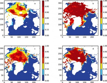
Fig. 3. Comparison of SIC for 15 July 2009 from (a) OSISAF, (b) ROMS Arctic-20km, (c) ROMS Arctic-20km-DA and (d) AMSR-E.
The modeled summertime SIE in the ROMS Arctic-20km is significantly overestimated (cf. Fig. 3b with a and d). Sea ice remains in much of the Arctic shelf seas (Kara, Laptev and Chukchi seas), Greenland Sea and Hudson Bay. The possible causes for such overestimation are numerous: bias in the atmospheric forcing, overestimation of the initial SIT, underestimation of the oceanic heat flux and underestimation of the sea-ice melting process. A check indicated that the initial SIT was generally below 1.5 m in the Arctic shelf seas and Hudson Bay and this seems to be a reasonable estimate. Thus the main problems are most probably in the atmospheric forcing, oceanic heat flux formulation and sea-ice thermodynamics. These will be investigated in a later study.
The modeled SIE in the simulation with assimilation, ROMS Arctic-20km-DA, is much improved, generally agreeing very well with the observations (cf. Fig. 3c with a and d). Interestingly, the modeled SIC is notably higher than the original OSISAF observations (which were used for data assimilation) and in very close agreement with the AMSR-E SIC. This is a significant improvement compared with the original OSISAF observations and also compared with the unchecked ROMS Arctic-20km during these summer conditions.
Discussion and Conclusions
We have introduced a simple and cost-effective assimilation scheme for SIC in the ROMS coupled sea-ice-ocean model. It is noted that the nudging weight G is a central parameter directly affecting the overall assimilation skill. In general, it should vary spatially and temporally and, more specifically, depend on both model and observation qualities. For more homogeneous fields such as atmospheric and oceanic variables, a constant value may work well. But for highly heterogeneous fields, such as sea-ice variables, the spatial and temporal variabilities generally cannot be ignored. We have provided an empirical method to account for such variability: G is split into two parts (Eqn (2)); one part is described by the optimal weighting K between model and observation error variances (Eqn (3)) and the other is described by a spatially and temporally varying timescale r (Eqn (4)).
The numerical experiments performed show that the COIN scheme provides a substantial and significant improvement on modeled SIC. Indeed the analyzed summer SIC is more in line with the AMSR-E observation than the OSISAF observation and significantly better than a free run with no assimilation. A similar method is presently being tested for assimilation of SST into ROMS.
The current ROMS system tends to overestimate SIE and SIC for the Arctic, as can be seen in both winter and summer simulations (Figs 2 and 3). Such overestimation would apparently affect the forecast of the sea-ice cover. As has been pointed out, it is most likely due to the bias in the atmospheric forcing, underestimation of the oceanic heat flux and overestimation/underestimation of the sea-ice growth/melting processes. Further study is required to clarify the source of this bias.
Acknowledgements
We thank the OSISAF High Latitude Processing Centre for providing the OSISAF sea-ice concentration data, and the Institute of Environmental Physics, University of Bremen, for providing the AMSR-E sea-ice concentration data. We thank Lars Petter Røed for helpful discussions, and anonymous reviewers for comments that helped improve the manuscript.


