

Introduction
Arctic Sea ice reaches an equilibrium thickness of 2–2.5m due to thermodynamic growth that depends on the energy fluxes between ice and both the ocean and the atmosphere (Reference Maykut and UntersteinerMaykut and untersteiner, 1971). further ice growth results from the ice motion as the ice cover deforms under convergent and Shear drift, causing rafting and ridging to take place. during rafting, when ice plates often thinner than 15cm Shift on top of each other, the floe Surface remains flat. when ridging occurs, the ice floes are crushed into blocks, which pile up. in the arctic Sea ice, ridging is of Scientific interest for two reasons. on the one hand, about two-thirds of the arctic Sea-ice volume reaches its thickness by dynamic deformation, which has an important impact on the fluxes of heat and momentum between atmosphere, ice and ocean. on the other hand, there is a growing interest in Shipping operations in the arctic ocean as the Sea-ice cover retreats, which demand improved forecast models including ridging.
In reality, ridges have a very complex Structure. they consist of a Sail above the water level and a keel below. however, a Sail is not always attached to a keel. ridges are very inhomogeneous. they consist of Single ice blocks that are fragments of the parent ice floes. during measurement campaigns on the ice that focus on Single ridges, the height and width of Sails and keels, Slope angles, block thicknesses and the volume of voids are Subjects of interest. apart from block thickness, which is related to the thickness of the parent ice floe (Reference LensuLensu, 2003), these parameters Serve to estimate the ice volume Stored in ridges. if investigations rely on profiles from airborne laser altimetry or underwater upward-looking Sonar profiling, ridge density (number of ridges per km) is the most important parameter along with Sail height or keel draft. thus, this Study focuses on these latter parameters.
In this investigation, a dynamic–thermodynamic continuum Sea-ice model, Similar to those routinely used in coupled climate Simulations, is applied. common arctic-wide models are based on the assumption that the Sea-ice cover is a two-dimensional medium. in Such models, ‘ridging Scheme’ most often denotes a numerical Solution to the problem that the ice concentration, which is ice area per gridcell area, might exceed unity (e.g. Reference SchulkesSchulkes, 1995). this happens because the contribution of vertical motion during ridging is neglected in the continuity equations. Reference HiblerHibler (1979) Solved this by including an artificial Sink term, in the continuity equation of the ice concentration, which is interpreted as ice area consumption due to ridging and Simply resets ice concentration A to unity if A > 1. because the mean ice thickness h, also referred to as ice volume, is conserved, the actual ice thickness h/A consequently increases.
Reference Gray and MorlandGray and morland (1994) proposed a Solution that incorporates the contribution of the vertical velocity component to the continuity equations of ice concentration and thickness. this term includes a So-called ‘ridging function’ r that adheres to the limits 0 < r < 1 and requires r→0 for A→0 and r→1 for A→1. no further constraints are explicitly identified and r might depend on A, h or principal invariants of the Strain rate (Reference SchulkesSchulkes, 1995). however, the ridging function prevents A from exceeding unity and regards ridging as having occurred when A < 1. in an equivalent approach, Reference ShinoharaShinohara (1990) also considers ridging during Shear ice motion. a different approach by Reference Thorndike, Rothrock, Maykut and ColonyThorndike and others (1975) introduced a model based on an ice-thickness distribution function to handle its dynamic growth. here, Sea ice is redistributed between discrete categories of ice thickness. the function conserves A and h and considers the different States of Sea-ice motion: divergence, convergence and Shear. Reference Flato and HiblerFlato and hibler (1995) extended this distribution model by Splitting the distribution function into two contributions: from level and ridged ice.
However, none of these models explicitly derives ridge parameters like those Specified above. if at all, ridged ice is characterized by ridged ice area fraction, volume or growth of volume (Reference Flato and HiblerFlato and hibler, 1991, Reference Flato and Hibler1995). three different, partly new, pressure-ridge algorithms are compared in this Study in an effort to find a realistic parameterization for the development of ridges in these comparatively coarse grid models. these are based on works of Reference Harder, Lemke, Johannessen, Muench and OverlandHarder and lemke (1994), Reference Steiner, Harder and LemkeSteiner and others (1999) and Reference LensuLensu (2003). first, the different algorithms and their historical background are briefly described. then they are tested under idealized conditions, using a dynamic Sea-ice model with Simplified geometry and forcing. finally, all algorithms are applied to the full arctic Sea-ice model, including thermodynamics, and compared to observational data from laser profiles of the Sea-ice Surface around Svalbard.
Data and Methods
Ridging models
In this Study, a dynamic–thermodynamic Sea-ice model with viscous-plastic rheology is used, which has previously been described in Reference HarderHarder (1996) and Reference Kreyscher, Harder, Lemke and FlatoKreyscher and others (2000). the dynamics of the model are based on the work of Reference HiblerHibler (1979), and the thermodynamics follow the model of Reference Parkinson and WashingtonParkinson and washington (1979). the model’s dynamics and rheology have been intensely evaluated (Reference Kreyscher, Harder, Lemke and FlatoKreyscher and others, 2000). the model has been used Successfully in arctic climate Studies over the last 50 years (e.g. Reference Hilmer and LemkeHilmer and lemke, 2000) and Sea-ice coverage forecasting (Reference Lieser, Lemke, Squire and LanghomeLieser and lemke, 2002). here, an ice class for deformed ice is introduced, which enables the model to differentiate between level and ridged ice. consequently three different algorithms describing pressure-ridge formation are implemented.
The first ridge algorithm (RA1) of Reference Steiner, Harder and LemkeSteiner and others (1999) introduces deformation energy R as a prognostic variable. its Source is the work done by the internal forces of the ice, and its Sink is a Simple melting term proportional to the thermodynamic change of mean ice thickness h. the ridge density D is proportional to the Square root of R/h. for the mean Sail height H, a cubic equation results from the only realistic Solution of the integral of the total potential energy of all ridges within a gridcell, assuming a constant ratio between Sail height and keel depth.
The Second ridge algorithm (RA2) is an extension of the redistribution model of Reference Flato and HiblerFlato and hibler (1991) and Reference Harder, Lemke, Johannessen, Muench and OverlandHarder and lemke (1994). here, convergent and Shear ice drift result in a transfer of undeformed ice to the deformed-ice category via a redistribution function in the continuity equations for level and ridged ice concentrations A l,r and mean thicknesses h l,r. this function is proportional to the invariants of the Strain-rate tensor and increases exponentially with the ice concentration. based on the redistribution results, ridge parameters are calculated by an embedded monte carlo model. Sail-height and ridge-length probability density functions of exponential Shape, which are derived from measurement data, are used in the Simulation of Single ridges. furthermore, ratios of Sail height to keel draft (1 : 4.5) and draft to width (1 : 4.0) for first-year ice (see Reference Timco and BurdenTimco and burden, 1997) are applied to derive Single ridge volumes. a triangular cross-sectional Shape is assumed for Sail and keel. Such Single ridges are formed until their geometric volume equals the redistributed ice volume per time-step and gridcell. average ridge density is derived proportional to the total ridge length per ice-covered area (Reference Mock, Hartwell and HiblerMock and others, 1972). initially in the idealized test Set-up, the mean Sail height H was derived from an arithmetic average of the mean height of already existing and newly formed ridges. it is then changed to be proportional to the Square root of level-ice thickness h l (Reference LensuLensu, 2003) because of the resulting large inconsistency of the field of Sail heights.
Based on the work of Reference LensuLensu (2003), in the third ridge algorithm (RA3) a ridging function as in Reference Gray and MorlandGray and morland (1994) is applied. this function reduces the (level) ice area and acts as a Source to ridge formation. its effect monotonically increases with ice volume because ridging takes place when the ice cover is compact and thick enough that rafting alone will not take place. furthermore, two prognostic equations for ridge density D and Sail height H are introduced. here, D represents the number of ridges per km without Spaces of open water. actually (AD) and (ADH) are treated in the two continuity equations. hence, D intensifies with a decrease in ice concentration A. new ridges are formed in response to the State of Sea-ice motion and a parameterization of the ice area consumption of a Single ridging event. the Sail height H depends on the formation rate of ridges used for D and the parent ice thickness, where the Same proportionality of h I, later applied to RA2, is used. the clustering effect, which reduces the cross-sectional volume of the Single ridges, is also taken into account. using another monte carlo model (M. lensu, unpublished information), a functional relationship between the equivalent ice volume Stored in the ridges and D and H is found. thus, through the evolution of ridge parameters, a redistribution of ice from the level to the ridged category is achieved. Reference LensuLensu (2003) designed basic parameterizations contained in this algorithm mainly for the relatively thinner ice of the baltic Sea.
In Summary, all of the three ridge algorithms presented here rely on the Strain rate as a result of differential ice motion, but differ in their implementation. RA1 is based on only one ice class, whereas RA2 and RA3 both use two ice classes. in RA2 the ice is first redistributed and ridge parameters are computed from the proportionate volume, whereas in RA3 the ridge parameters are treated as prognostic variables and thus control the formation of the ridged ice volume.
Observations
Observations from Several expeditions to the arctic from 1995 to 2004 are used (personal communication from c. haas, 2006). these data are airborne laser profiles mainly in the area of the transpolar drift Stream from the laptev Sea to fram Strait. to a lesser extent they were also obtained in the kara, lincoln and beaufort Seas. from the laser profiles, ridge parameters are derived using the So-called rayleigh criterion (Reference DierkingDierking, 1995). for consistency with the model results, the data are averaged into 25 km bins. in particular, data from rv Polarstern cruise ark xix to the barents Sea and the fram Strait region in march and april 2003 provide a unique Set of ridge parameters before Summer melt Starts, So the final comparison focuses on these.
Experiments
1. in order to test the behaviour of the three ridge algorithms in a controlled environment, a Simplified model configuration is chosen. ridge formation is an entirely dynamic process. hence, thermodynamics are turned off in these tests. the model is applied to an idealized rectangular domain with a horizontal grid resolution of 40 km to be consistent with Reference Haapala, Lönnroth and StösselHaapala and others (2005). a time-step of 2 hours is chosen. the Sea-ice model is forced with a wind field typical of a northern hemisphere cyclone. a depression of 970 hpa with a cosine gradient towards 1000 hpa normal pressure is used to calculate the geostrophic wind. the cyclone is centred on y coordinate 15 with a diameter of 640 km and moves with a constant velocity of 480 km d–1 to the east (see fig. 1a). two runs with different geometries are performed. in the first run, the model grid is free from any topographic obstacles, while in the Second run a peninsula, which is centred on x-grid point 33 with a foot width of 18 gridcells at the boundary, is protruding from the north into the course of the cyclone (illustrated in fig. 1). both runs Start with an initial level-ice cover of 0.5 m thickness and 95% concentration and without any ridged ice.

Fig. 1. (a) Sea-ice drift field of the idealized cyclone experiment. The large arrow indicates the direction of motion of the cyclone. (b) Sea-ice concentration decreases on the track of the cyclone. The black area marks the topographic obstacle (peninsula). Axis labels represent gridcell numbers; x is taken as west–east and y as South–north direction. Gridcell width is 40 km.
2. next the three ridging algorithms are tested under realistic arctic conditions. for this purpose, the uncoupled Sea-ice model is integrated on an arctic-wide rotated grid with a Spatial resolution of 1/4˚ (27.8 km) and a time-step of 6 hours. at every time-step the air temperature (at 2m height) and winds (10 m) from european centre for medium-range weather forecasts (ECMWF) 6 hourly re-analysis data are prescribed. all oceanic and further atmospheric forcing fields are monthly mean climatologies. in contrast to the idealized cyclone experiments, the model uses the full thermodynamics.
3. the comparison to observations Starts by contrasting the laser profiling data from march–april 2003 with the ridge parameters derived from one of the ridge algorithms (RA2) on a map. in order to extend this comparison to RA1 and RA3, results of all three ridge models are plotted as a function of laser data from march and april 2003. a nearest-neighbour algorithm is used to derive the corresponding values from the gridded model data. in addition to the median values, Squared errors (Dmod–Dobs)2 are used as an objective measure for the discrepancy between each of the modelled estimates and the corresponding observed value. hence, at each geographical location one of the three ridge algorithm results matches best, i.e. has the Smallest Squared error. this gives a ‘hit rate’ for each algorithm, denoting its quality.
Results
Idealized test
In the first run of this experiment (not Shown), all three ridge algorithms lead to the Same pattern in ridge density. along the track of the cyclone, there is no variation. across the track, maxima occur towards northern and Southern track edges, with the Southern maximum more pronounced, and lower density in between. these findings can also be Seen in the results of the Second run (fig. 2a–c), because the results of the two runs differ only at gridcells with x coordinates 15–45. the maximum ridge density coincides with the lowest ice concentration (fig. 1b Shows ice concentration of RA2). more interesting is the Second run with the presence of a topographic obstacle (figs 1 and 2; x gridcells 33±9). the along-track homogeneity is lost in all three cases. the Spatial distribution is perturbed before and behind the obstacle. on the western Side of the peninsula the ice is driven off the coast and a reduced ice concentration is left behind. on the other Side of the peninsula, where the wind blows onshore, intense ridging occurs in all three models. however, the Strongest ridge formation is computed with RA1, where values above 0.06 km–1 are reached across the track.
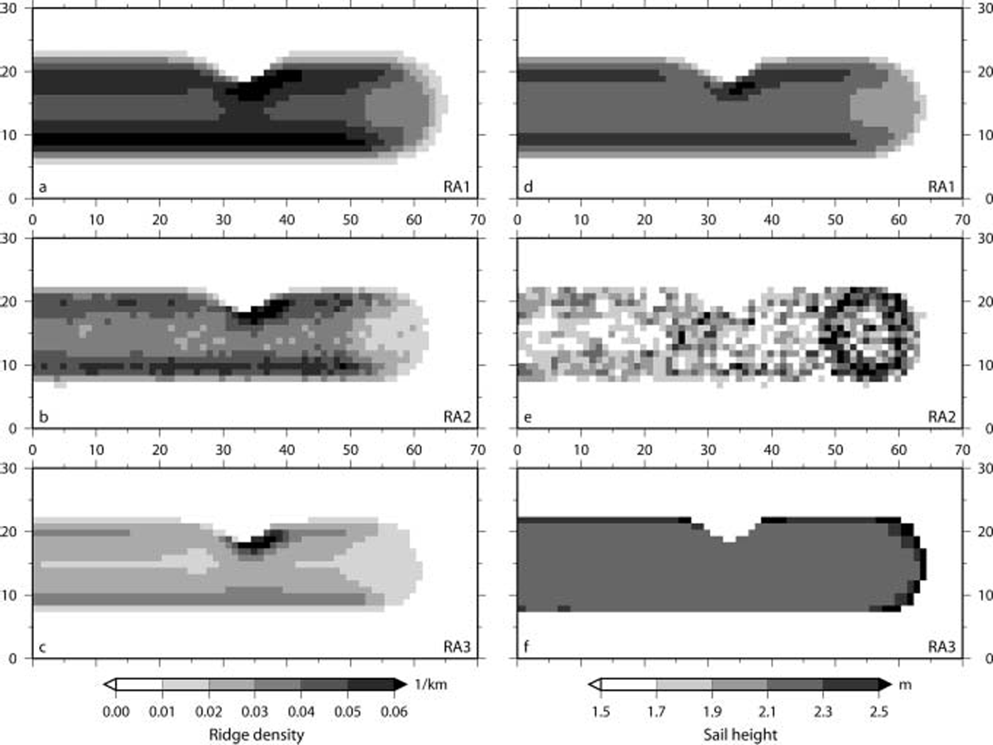
The mean Sail heights computed by the three ridge algorithms are close in the range (within ∽0.5 m), but there are pronounced differences in their Spatial distribution (see fig. 2d–f). for RA1 the mean Sail height closely follows the ridge density, with largest heights where most ridges form. the results of RA2 contain a lot of noise and are therefore difficult to interpret. the most remarkable feature of the results of RA2 is the presence of the largest Sail heights at the position of the cyclone. the distribution in the wake of the cyclone follows the unperturbed ridge density. RA3 leads to a very homogeneous distribution, with an increase in mean Sail height of up to 40 cm towards the rims of the ridging zone, especially in front of the cyclone.
Model comparison over the Arctic Ocean
Here the three ridging algorithms are compared with each other with respect to realistic arctic conditions. figure 3 presents the model results in mid-winter, averaged over march 2003, when most of the winter ridge formation has happened. all ridge algorithms produce realistic ridge densities (0–30km–1) and Sail heights (up to 3 m). the ridge density distributions closely follow the topography, because the most intense convergence and Shear occurs along the coastlines, especially north of the canadian arctic archipelago and greenland. areas of <5 ridges per km in the laptev and east Siberian Seas are partly attributed to fast ice, which is implemented in the applied Sea-ice model via the grounding of ice in these Shallow Shelf Seas. far from the coast, the ridging models RA1 and RA2 feature ridge densities of more than 10 or 15 km–1 whereas RA3 Stays below 10km–1. these differences are also evident in the medians of the distributions (see table 1). the fact that RA2 has the largest Standard deviation in D (10.1km–1) is linked to the presence of the most pronounced gradient of D across the arctic basin in this model. however, all model Sail heights have nearly the Same Standard deviations (see table 1) and the patterns are less pronounced. again RA1 and RA2 have larger values (+0.5 m) than RA3 in most areas.

Fig. 3. Ridge density D (km–1) (a–c) and mean Sail height H (m) (d–f) computed with ridge algorithms RA1–RA3 applied to realistic Arctic conditions. Average values of March 2003 are Shown.
Table 1. Median and Standard deviation (stdev) of the modelled ridge densities D and the mean Sail heights H computed from the mean of March 2003. The corresponding model results are presented in Figure 3

Comparison to observations
In general, the observational data Show a very consistent ridge distribution in the area of the transpolar drift Stream, with a moderate Sail height of 1.3 m on average. extensive ridging occurs towards the coasts of greenland and the canadian islands (1.6 m), whereas the ridges are Smallest in the beaufort and laptev Seas (1.1 m). all of the three ridge models Simulate this gradient in ridge intensity across the arctic basin. however, at first Sight the results of RA2 Seem to resolve various patterns best. hence, these model results are presented together with the observations around Svalbard in figure 4. as expected, ridge density is reproduced well by RA2. the flat Surface of the newly formed ice of refrozen coastal polynyas inside the Storfjord and the tongue of highly deformed multi-year ice (20–40 ridges per km) Stretching out from the central arctic, blocking the outlet of the Storfjord, are completely reproduced by the Simulations. further, in the barents Sea the model results are very Similar to the uniform distribution of measured Sail heights (±0.1 m). results in fram Strait match less well.

Fig. 4. Ridge density D (km–1) (a) and mean Sail height H (m) (b) derived from ridging algorithm RA2 and laser profiling. Contours Show RA2 results from 31 March 2003, and filled circles represent observations from March (Barents Sea) and April (Fram Strait) 2003 averaged over 25 km bins.
Presenting a comparison of all model results to the observations, figure 5a–c Show that the models tend to overestimate the ridge density. this is underlined by the medians of the differences between modelled and observed values (see table 2). the Squared errors reveal that the ridge densities of RA3 are closest to observations in 59% of all locations. the Sail-height estimates agree reasonably well with the observations. RA1 (fig. 5d) tends to have larger Sails, underlined by a comparatively large positive median of Sail height difference (0.25 m; See table 2). furthermore, this algorithm leads to the most evenly distributed Sail heights (not Shown), which becomes obvious in the Smallest variance of all, 0.02 m2. in contrast, RA3 (fig. 5f) underestimates larger Sail heights attributed to fram Strait by up to 50 cm. the results of RA2 match the observed Sail heights best (fig. 5e). this is Supported by the highest hit rate of Squared errors, 69%.

Fig. 5. Comparison of Simulated and observed ridge density D (a–c) and mean Sail height H (d–f) in March–April 2003 at coincident model gridcells and laser flight leg locations. Samples from Fram Strait are marked as diamonds. The grey lines are 1/1 lines.
Table 2. Results of the Statistical analysis of the differences in ridge density D and mean Sail height H between modelled and observed values, which are presented in Figure 5

Discussion
Idealized test
The tests Show that the initial ice concentration of 95% is reduced by up to 1% (see fig. 1b) due to the Strong winds in the cyclone. this is in good agreement with the findings of Reference Haapala, Lönnroth and StösselHaapala and others (2005). as a consequence of the Stronger ridge formation (+0.02 km–1), the deformation process consumes more level-ice area in RA2 than in RA3. thus the cyclone leaves more open water with RA2 (+0.3%).
In general, the algorithms are made for reproducing the ridge density formation in the arctic for a whole winter Season. therefore it is not astonishing that the total number of ridges arising from a Single cyclone event is less than 1 ridge per 10 km. while ridge densities of all three algorithms are reliable, only Sail heights of RA1 and RA3 Seem to be equally appropriate for further experiments. the noise in the RA2 data is due to the monte carlo Simulation that is part of this algorithm. therefore, a different approach, that regards Sail height proportional to the Square root of the parent level-ice thickness (Reference LensuLensu, 2003), is used to improve the Sail heights. although this approach results in a uniform Sail height distribution in the idealized tests, its practicability is Shown in the application to the realistic arctic Sea-ice cover in experiment (2).
Model comparison over the Arctic Ocean
Summarizing, the ridge density depends Strongly on the topography and the State of ice motion, while ridge Sail height depends less on the topography but more on the mean (level) ice thickness. of course, the Sail heights of RA2 (fig. 3e) almost resemble the typical ice-thickness distribution, known from observations and many Simulations, because of the direct functional relationship. although Sail-height derivations in RA1 and RA3 are equally unrelated to ice thickness, the Spatial distribution of the RA1 results is close to that of RA2. in contrast, Sail-height distribution from RA3 is Strongly related to the ridge density. this gives RA3 the capability of generating distinct Sail heights along the coastlines and the fast-ice edge, that are properly distinguished from the deformation of the fast ice itself (see fig. 3f, near the new Siberian islands). this algorithm also features large ridge densities of >30km–1 in the marginal ice zone, especially in the greenland and barents Seas (fig. 3c). these result from the treatment of D as density along a profile excepting leads. in this case, D represents the highly deformed (multi-year) ice floes, which drift in a region of common Storm tracks.
From all results of modelled ridge density, those of RA2 exhibit the most pronounced pattern, featuring for example the beaufort gyre (fig. 3b). this has to be Seen as a result of the well-proven redistribution function included in RA2, and less attributed to the ridge formation itself. with the adjusted formulation for Sail height, a relatively homogeneous field is achieved. concluding, this algorithm is Suggested for climate Studies. in contrast, RA3 is Suggested for regional, Short-term forecast models (e.g. for Ship routing) because the ridging processes Seem to be most limited in their extent and best resolved near the coasts.
However, the homogeneous distribution of the mean Sail height does not represent the Small-scale variability of a ridged area. incorporating experience from observations, large variations of Sail height occur mostly on a Scale which cannot be resolved by the model grid used here.
Comparison to observations
The behaviour of the models in fram Strait needs to be discussed here, as this region is obviously difficult to Simulate. ridge density is Slightly overestimated and unrealistically constant. in addition, the heterogeneity of measured Sail heights is missing. in RA3, fram Strait Sail heights are underestimated due to the less intense ridging activity offshore. outliers in figure 5f (H RA3 values <0.5 m) are located inside the Storfjord, where RA3 almost completely overlooks the observed ridge formation. the models do not reproduce the diversity exhibited by observations for two reasons: (1) the Simulated ice drift has less variability than observed, because the ice is funnelled into fram Strait, and (2) the deformation features observed in fram Strait originate from the entire arctic basin, and floes might have undergone Several deformation processes depending on their age. to date, these multi-year features are not adequately treated in the ridging algorithms.
However, the conclusions drawn from the comparison of the different model results with observations have to be discussed carefully, because the Selected observational data cover only a Small part of the arctic at the end of one winter Season.
Conclusions
For the first time, different pressure-ridge formation Schemes are compared with each other and to observations. the basis for this investigation is an uncoupled continuum dynamic–thermodynamic Sea-ice model. many of the numerical models of this type use a Simplified deformation Scheme, especially in coupled mode. this needs to be improved. for climate Studies, ridge algorithm RA2 Seems to be most appropriate, as it generates inner arctic patterns most accurately, including gradients already known from former Studies. in addition, this model applies a redistribution Scheme between ice classes as already used in multi-category Sea-ice models. for Sea-ice forecasting and decision-making in Shipping operations, RA3 is preferable as nearshore features and fast-ice related characteristics are resolved best. these are of Special interest along the northern Sea route. in addition, deficiencies of this algorithm, Such as the redistribution of ice volume and area and the conservation of ice mass, are less important, because forecast periods would not extend further than 1 week and would be combined with assimilation of observations. these recommendations are restricted for the following reasons: (1) the Set of observational data is limited, (2) an uncoupled Sea-ice model is used, i.e. the driving ocean currents are limited to the climatological monthly means, and (3) the ridges that are created have no feedback within the System, for example on the atmospheric or oceanic form drag.
The calculation of ridging parameters in numerical Sea-ice models offers new opportunities for model validation (e.g. the comparison with ridge parameters derived from remote Sensing). a next Step in modelling will be the development of an advanced fast-ice Scheme, which uses the newly implemented ridging values for a more exact grounding Scheme. also the possibility of calculating atmospheric and oceanic drag coefficients that are dependent on the ridge density and height will be investigated. multi-category Sea-ice models, which have been developed and improved in the past decade, are used to an increasing extent. the advantages and disadvantages of these redistribution models need to be investigated more closely. yet before this can be done, it is necessary to focus on the changes in the Structure of ridges during the Summer Season, and the decay of the ridge density and height due to melting processes and fragmentation of floes. however, the formulation of pressure-ridge formation, which is most Significant in the winter Season, can Successfully be included in numerical (un)coupled Sea-ice models.
Acknowledgements
This Study is part of the european union project iris (ice ridging information for decision making in Shipping operations), contract no. EVK3-ct-2002-00083. most laser profile data are kindly provided by c. haas. thanks to c. haas, j. haapala, m. lensu, r. timmermann and l. axell for many fruitful discussions. the comments of the two anonymous reviewers and the remarks of the Scientific editor p. langhorne helped to improve the manuscript.


