Satellite-derived data

Satellite-derived Polar Pathfinder sea-ice motion vectors, a merged product of drift vectors from SMMR (1978–87), SSM/I (1987–2006) and AVHRR (1981–2000) images (http://nsidc.org/data/nsidc-0116.html), are provided by the US National Snow and Ice Data Center (NSIDC). Drift velocities are obtained by a maximum cross-correlation method, using daily composites of brightness temperature fields from the vertical and horizontal polarization of the 37GHz (SMMR and SSM/I) and the 85.5 GHz channels (SSM/I), as well as signals of the visible and thermal channels of AVHRR data, to calculate displacement vectors for special patterns, which have high correlation between sequential days (e.g. Reference Ninnis, Emery and CollinsNinnis and others, 1986; Reference Emery, Fowler, Hawkins and PrellerEmery and others, 1991).

The derived drift vectors of each sensor are merged by an optimal interpolation method for all areas where ice concentration exceeds 50% (Reference Fowler, Emery and MaslanikFowler and others, 2001). This method results in ice-drift fields without gaps. Data are provided with a daily resolution and have a spatial resolution of 25 km, showing the mean large-scale displacement vectors on a regularly spaced grid from November 1978 until December 2006. the drift vectors are georeferenced to an azimuthal equal area projection and positions are given in grid coordinates. In contrast to the Arctic sea-ice motion product, these Antarctic sea-ice motion fields do not include buoy data, so this product is independent of those used for the comparisons made in this study.

The advantage of the Eulerian drift fields is the large-scale coverage. However, temporal and spatial resolutions are limited to a resolution of 25 km for the 37 GHz channel and about 12.5 km for the 85.5 GHz channel. In addition, composed brightness temperatures for 1 day are obtained from overpasses of different times and also different locations per day, which could smear or blur the brightness temperature fields (Reference Kwok, Schweiger, Rothrock, Pang and KottmeierKwok and others, 1998). A further problem is the sensitivity to high water content in the atmosphere of the 85.5 GHz channel. Under unfavorable conditions, this could lead to an interpolation of only a few drift vectors onto large areas of the grid and therefore to an over-representation of the interpolated drift regime.

The AVHRR has a higher temporal and spatial resolution. Up to four passes are used for daily composites, when available. In addition, AVHRR has a wide swath (>1000 km) and a high resolution of about 1 km. Unfortunately, this sensor is highly sensitive to clouds and atmospheric water vapor (http://nsidc.org/data/nsidc-0116.html; Reference Heil, Fowler, Maslanik, Emery and AllisonHeil and others 2001); therefore, data are only available for days with clear-sky conditions, resulting in many data gaps and probably in an under-representation of ice-drift regimes under any less favorable weather conditions. For more information on the merged sea-ice drift dataset see http://nsidc.org/data/nsidc-0116.html.

Drifting-buoy data

Polar Pathfinder sea-ice motion vectors were compared with vectors obtained from drifting buoys deployed on ice floes. the positions of those buoys were usually observed several times per day and were transmitted to the Argos satellite communication system. Two different types of position data are available. Earlier buoys were located by the Argos system using Doppler range finding (Reference Heil, Fowler, Maslanik, Emery and AllisonHeil and others, 2001). the accuracy of these positions is approximately 0.5 km (Reference Emery, Fowler and MaslanikEmery and others, 1997; Reference Harder and FischerHarder and Fischer, 1999). Since 1997, newer buoys have included GPS receivers, resulting in position accuracies of better than 50m (Reference Heil, Fowler, Maslanik, Emery and AllisonHeil and others, 2001). Using the position data, drift vectors were derived and have been projected onto a regular hourly time grid, with the exception of the data since 2001, which were provided as 3 hourly position records. To allow for a comparison with the satellite-derived ice motions, which were derived from changes in daily composites of image patterns of sequential days, the hourly spaced buoy drift vector components were averaged into daily mean values using the data from 0000 h to 2400 h every day, centered on 1200 h.

The buoy ice-drift dataset provides Lagrangian drift trajectories with high spatial and temporal resolution as well as high accuracy but with limited spatial and temporal coverage. the spatial distribution of the buoy data, available for 1989–1999 and 2001, 2002, 2004 and 2005, is shown in Figure 1 , with initial positions of all buoys used for this study. the number of buoys deployed varied from maximum values of 15 in 1989, 13 in 1992 and 11 in 1996/97 to a minimum of three buoys in 2004/05 and only one buoy in December 2001. Data are obtained from various sources. Most data are provided by the Alfred Wegener Institute; these are available on the Pangaea website (http://www.pangaea.de/search?count=108Jq=Buoy+Weddell+sea++) Some other buoy data were provided by the International Programme for Antarctic Buoys.

Fig. 1. Distribution of buoy start positions between 1989 and 2005 (symbols) and their drift tracks (gray lines). See Table 1 for region abbreviations.

Data processing

To compare ythe two datasets, a bilinear interpolation of the daily mean satellite-derived zonal and meridional ice-drift components onto the daily mean buoy positions has been performed. Interpolation was done only when all velocities from surrounding gridpoints were available. Consequently, some data near the ice edge had to be excluded and quality analysis is not included for this region.

Because the satellite-derived drift vectors are given in grid coordinates, they had to be rotated based upon their longitude to obtain the zonal (east–west) and meridional (north–south) drift components at the daily mean buoy positions. Afterwards, differences for both drift components were calculated by subtracting the satellite-derived from the daily mean buoy-derived ice drift. the statistical significance of differences and correlation coefficients was proved using a t test (e.g. Reference Press, Teukolsky, Vetterling and FlanneryPress and others, 2007).

In total, there are 11 928 coincident drift vector pairs for the study period. the number of data points used to calculate yearly means varies strongly, depending on the number of buoys deployed in one particular year and the number of available satellite-derived ice-drift vectors for the buoy positions. For example, in 1990, 12 buoys were operated, but the number of corresponding drift vectors from the two datasets is only n = 58. the reason for this difference is most likely the operating region (northern part, near ice edge) in conjunction with the season (beginning in January) of the respective buoys. the connections between regions, season and number of data points with the agreement between buoy- and satellite-derived ice drift is reviewed in the discussion. the maximum number of corresponding drift vectors in one particular year is 2010, obtained in 1996, when 11 buoys were deployed. Contrary to the yearly distribution, the number of monthly data points is relatively high and varies between a minimum of 440 in January and a maximum of 1425 in October. In late spring, summer and early fall a higher number of buoy data are available than the number of coincident buoy- and satellite-derived vectors would suggest. This often occurred when buoys were located near the ice edge, especially when records were started in summer. A reasonable explanation is that satellite-derived ice drift was only calculated when ice concentration was >50%. In addition, satellite-derived data close to the ice edge have been excluded from this study by the interpolation method. Therefore, some gaps can arise from the satellite-derived product for regions with lower ice concentrations where buoy-derived ice drift was still present. This would result in an earlier record of buoy-derived ice drift in fall and a longer record in spring compared with satellite-derived ice drift. an example is shown in Figure 2 . This means that the number of coincident drift vectors is not only dependent on the number of deployed buoys but also on the ice concentration for which ice-drift vectors are calculated from satellites.

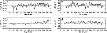
Fig. 2. 5 day running mean of buoy- (black) and satellite-derived (gray) zonal (a, c) and meridional (b, d) ice drift. Examples for a buoy in 1996 (a, b) and one in 1999 (c, d) are shown.

For an analysis of the different regions described in Table 1, n varies strongly, with minimum values of 0–29 and a maximum of 688 in the north-centralWeddell Sea. Hence, the number of corresponding data points contributing to mean values is highly dependent on the number of deployed buoys, the region and season of deployment and the ice concentration range used for satellite-derived ice-drift calculations.

Table 1. Definition of different regions for local comparisons

Overall comparison

The daily mean buoy drift speed of all 11 928 data points was 0.135 ms^–1, comparable with studies by Reference FischerFischer (1995), Reference Harder and FischerHarder and Fischer (1999) and Reference Kottmeier and HartigKottmeier and Hartig (1990) who observed typical drift velocities of 0.10–0.15ms^–1. the mean error of the buoy-derived daily ice drift is about 0.006 ms^–1 for older buoys with location accuracy of approximately 0.5 km and 5.9×10^–4ms^–1 for GPS drifters. the mean daily satellite-derived ice-drift velocity was 0.088ms^–1 for the same data points. This is 34.5% less than the mean buoy drift. the difference between the two datasets is significantly different from zero at the 95% confidence interval. of the satellite-derived ice-drift velocities, 71.1% are below those observed by buoys (not shown). This finding is similar to results from Reference Heil, Fowler, Maslanik, Emery and AllisonHeil and others (2001) who found that satellite-derived ice-drift speeds are generally lower than those derived from buoys for the East Antarctic sea-ice zone. Only 10.85% of the satellite-derived drift velocities are within a range of ±10% of the buoy-derived drift velocities. Nevertheless, it also occurs that the velocities exceed those observed by buoys.

Figure 3 shows the distribution of differences between buoy- and satellite-derived ice drift for all data from 1989 to 2005 for the zonal (u; east–west, positive in eastward direction) and meridional (v; north–south, positive in northward direction) drift components. Mean buoy-derived drift components are u = 0.012 ±0.112 ms^–1 and v = 0.038 ±0.115ms^–1. the mean satellite-derived drift is u = 0.000 ±0.072ms^–1 and v = 0.027 ±0.079 ms^–1. the mean differences between the two datasets, calculated by subtracting the satellite- from the buoy-derived drift, are significant at the 95% confidence interval with Δu = 0.012±0.091ms^–1 and Δv = 0.010±0.091ms^–1. Generally, differences of the meridional drift have a wider range than those of the zonal drift and the modal value for differences between buoy- and satellite-derived drift is 0.020ms^–1 (Fig. 3). For the zonal drift, the range of differences is lower and the modal value is –0.010ms^–1. the absolute differences (buoy – satellite) are 0.062 ±0.067 ms^–1 for the zonal and 0.065 ±0.064 ms^–1 for the meridional drift. Correlation coefficients, r, between daily buoy- and satellite-derived data are 0.59 for the zonal and 0.61 for the meridional drift (Fig. 4).

Fig. 3. Differences between buoy- and satellite-derived drift for (a) the zonal (u) and (b) the meridional (v) drift component. Bin size is 0.005 ms^–1. Pairs of buoy and satellite drift vectors: 11 928. Time period: 1989–2005. the two datasets and the number of data points, n, that contribute to the mean values. Furthermore, the 95% confidence interval for the differences is added and indicates where mean differences are not significantly different from zero. the magnitude of both drift components shown in Figure 5 is generally too low for the satellite-derived sea-ice drift.

Fig. 4. Correlation between buoy data and satellite-derived drift for (a) the zonal (u) and (b) the meridional (v) component. Pairs of buoy and satellite drift vectors: 11 928. Time period: 1989–2005.

Temporal and regional variability of differences between datasets

As buoys are unevenly distributed in time and space, data have been analyzed separately according to their temporal and regional distribution. In the beginning, all the data from one year are averaged into a yearly mean. In addition, data are averaged monthly for all years to study seasonal variations.

Figure 5 displays the yearly (Fig. 5a and b) and monthly (Fig. 5c and d) mean zonal (Fig. 5a and c) and meridional (Fig. 5b and d) drift speed, the averaged differences between

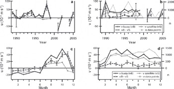
Fig. 5. Mean values for (a, c) zonal and (b, d) meridional components of buoy- (black) and satellite-derived (gray dotted line) drift, mean differences (gray, dashed line) with attached 95% confidence interval and number of corresponding drift vector pairs (n, light gray, only in (b) and (d)). (a, b) Yearly and (c, d) monthly distribution.

For the meridional drift component, the characteristics of the satellite-derived ice drift are comparable with those of the buoy-derived ice drift and deviations are <50% in most years (not shown). In contrast, deviations between the two datasets of the zonal drift component are often >50% of the buoy-derived ice drift, and in some years (e.g. 1996, 1998) the satellite-derived component has the opposite direction of the buoy drift.

Correlation coefficients between daily drift velocity components derived from satellite data and from drifting buoys for single years (Fig. 6) vary between about 0.4 and 0.7 for both drift components. an exception was 1998, when correlation between buoy- and satellite-derived zonal drift was low and negative, with a value of only –0.1, and low but positive at 0.34 for meridional drift. Furthermore, in 1990 and 2001, correlation coefficients between buoy- and satellite-derived meridional drift were only 0.24 and –0.25. the year 2001 even had a strong negative correlation for the meridional drift component. In those years, correlation coefficients are not significant at the 95% confidence interval. Possible reasons for this are given in the discussion.

Fig. 6. Correlation, r, between zonal (black) and meridional (dark gray, dashed) components of buoy- and satellite-derived ice drift. (a) Yearly and (b) monthly distribution. Gray bars show the region of <95% confidence for the correlation coefficients being nonzero.

Towards the end of the study period, absolute differences between buoy- and satellite-derived data decrease (not shown). For the zonal component, absolute deviations decrease by about 0.034ms^–1 (47%) and by about 0.030ms^–1 (41%) for the meridional drift during the study period. Additionally, the standard deviations of differences decrease, suggesting that the more recent satellite-derived ice-drift data are of higher quality.

As yearly discrepancies and correlation coefficients of buoy- and satellite-derived drift show high variation from year to year and the buoys are not distributed regularly in time and space, an analysis of accuracies on a yearly basis cannot sufficiently explain which factor, the temporal or the regional distribution, affects the accuracy of this particular satellite-derived dataset. Therefore, a seasonal as well as a regional study has been performed.

For the seasonal analysis, monthly averages were derived over the study period. Figure 5c shows that the mean prevailing zonal drift direction changes in July from westward (negative) to eastward (positive). the highest mean zonal drift speed of 0.057ms^–1 (buoy) and 0.017ms^–1 (satellite) was observed in October, while the highest mean meridional drift speed of 0.057 ms^–1 (buoy) and 0.044 ms^–1 (satellite) occurs in April. Between July and November and also in January, differences between zonal buoy- and satellite-derived ice drift exceed 50% of the respective buoy-derived zonal ice drift (Fig. 7). the differences of the meridional drift component (Fig. 7) vary between 10% and 50% of the respective buoy-derived ice drift for all months, except in January. the lowest discrepancies, <33%, occur from March through October. This means that the meridional drift component is somewhat more accurate from fall until mid-spring, while zonal drift discrepancies between buoy- and satellite-derived data start to increase in mid-winter (July; Fig. 5 and 7) and are highest in November (end of spring).

Fig. 7. Percentages of mean differences between buoy- and satellite-derived drift components (zonal: black, meridional: gray, dashed) for monthly distribution. Circles indicate that the confidence for differences being nonzero is <95% for each drift component.

Correlation coefficients for the monthly separated daily mean drift velocities (Fig. 6b) vary little between 0.4 and 0.8, except in January when the correlation is about 0.2 for both the meridional and the zonal ice drift. All of them are statistically significant at the 95% confidence level. In most cases, the differences in correlation between buoy- and satellite-derived drift for zonal and meridional drift are <0.1. Mean summer correlations (October–February, without the January correlation) are about 26% (u) and 16% (v) lower than winter mean correlations (March–September). the correlation coefficient in January is only about 0.24 (u) and 0.22 (v) for the ice-drift components, and therefore 63.0% (for zonal drift) and 66.5% (for meridional drift) lower than winter mean correlations. the fact that the October– February correlations are somewhat lower than those for March–September and that differences between the two datasets for both drift components are generally high from October to February may be due to sudden emissivity changes resulting from snow wetting, as described by Reference Willmes, Bareiss, Haas and NicolausWillmes and others (2006, Reference Willmes, Haas, Nicolaus and Bareiss2009), which can result in a loss of tracking features between sequential days. Furthermore, flooding events may change observed patterns from one day to another. These interactions may result in a reduction of satellite-derived ice-drift vectors and therefore in a wider interpolation of drift velocities.

Data have been separated into the six regions listed in Table 1 to study deviations between different regions. Monthly variations of correlation coefficients for each region are shown in Figure 8 . All regions have low correlation coefficients in January, which are mostly insignificant. This can be seen from the gray bars in Figure 8 , which show the region of <95% confidence for the correlation coefficients. Where the data points lie between these gray bars, results are not significant. In all other months, correlation coefficients show higher variations between about 0.4 and 0.8, which are comparable with the correlation coefficients obtained for the entire Weddell Sea shown in Figure 6 . It is remarkable that the same declining behavior is seen for the north-central and northeast parts, where correlation coefficients start to decrease slightly in early spring, which could be a result of surface melt. For the eastern part of the Weddell Sea, mean correlation is <0.5 for both drift components in the southern part, while other regions have a mean correlation coefficient higher than 0.5. the September correlation of the meridional component is even negative in the southeastern Weddell Sea, but is statistically insignificant at the 95% confidence level. Again, there seems to be a relation with the number of corresponding data points contributing to the correlation calculation, which was only 16 for September in the southeast region. However, the low mean correlation for the southeastern Weddell Sea is a result of the low September correlation of 0.04 (u) and –0.1 (v). Excluding these values, the mean correlation from January through August is >0.5. Furthermore, the averaged September vectors are all obtained in just one year, namely 2004. Therefore, this value represents only one month and not a long-term monthly mean and cannot be compared with other correlation coefficients in the same way that the long-term means are compared. Finally it seems that the correlation coefficients do not significantly vary between different regions in the Weddell Sea.

Fig. 8. Correlation between zonal (black) and meridional (dark gray, dashed) components of buoy- and satellite-derived ice drift for monthly separated data and number of corresponding drift vector pairs, n (light gray), for different regions. Gray bars show the region of <95% confidence for the correlation coefficients being nonzero.