


1. Introduction
Airborne radar remote sensing is an effective tool in geoscience fields for conducting Earth observations. As compared to ground base and satellite-based methods, airborne remote sensing offers significantly larger spatial coverage than ground-based methods and the ability to conduct finer-grid measurements than satellite-based methods. In radioglaciology, airborne measurements also offer a potentially safer option than in situ field measurements. Over the last 30 years, researchers at the University of Kansas (KU) have developed a series of airborne radars for ice and snow measurements; over the last 15 years, technology developments have included several unmanned aerial systems (UAS) for polar remote sensing. In 2005, KU led the effort to join with researchers from other universities and organizations to form the Center for Remote Sensing of Ice Sheets (CReSIS), whose goals included developing new technologies to meet the needs of the polar science community.
The radar systems developed by CReSIS can be organized into four major categories: radar depth sounders (RDS), accumulation radars, snow radars and radar altimeters. These radars cover a wide frequency range (14 MHz to 38 GHz); together, they provide a vertical profile of the entire ice column with various degrees of resolution. The radars are capable of detecting air/ice, ice/snow and ice/bedrock interfaces due to the difference in dielectric constants of the various media. Internal layers that are apparent in radio echograms are a result of electromagnetic wave reflections attributed to density changes for depths <200 m (Paren and Robin, Reference Paren and Robin1975; Arcone and others, Reference Arcone, Spikes, Hamilton and Mayewski2004) and conductivity changes at depths >200 m (Millar, Reference Millar1982; Hempel and others, Reference Hempel, Thyssen, Gundestrup, Clausen and Miller2000). Changes in the crystal orientation fabric throughout the ice column also influence the dielectric constant of ice (Fujita and others, Reference Fujita, Matsuoka, Ishida, Matsuoka, Mae and Hondoh2000). The frequency of operation for each of the radar systems is determined by the ice/snow properties to be measured, and specific frequency bands are driven by radar system limitations and frequency allocation. Systems operating in the very high frequency (VHF) spectrum or lower are used when the depth of penetration is a driving requirement (such as for bedrock imaging) due to their reduced sensitivity to ice attenuation and scattering (Paden and others, Reference Paden2005). When a finer resolution is required (e.g. measurement of centimeter-thick snow on ice), it is advantageous to operate with a much higher center frequency where high bandwidths, and thus improved resolution, can be achieved. CReSIS RDS – designed to measure bed topography and ice thickness – operate over 14–600 MHz. The accumulation radar, used to measure shallower bed topography and internal layering, operates over the 600–900 MHz frequency range. The snow radar, which operates over 2–8 and 2–18 GHz, measures snow cover and near-surface internal ice layering. Finally, the radar altimeters operate over 12–18 GHz (Ku band radar) and 32–38 GHz (Ka band radar); they are used to measure surface topography and near-surface layering. Table 1 provides an overview of the aforementioned radar systems.
Table 1. Overview of CReSIS radar systems

Over the last decade, we have flown these systems on a variety of both manned and unmanned aircraft as well as operated on multiple surface-based platforms. Figure 1 provides an overview of most of the aircraft on which the radars have been integrated (there are a few configurations that have not been included in the graphic due to space). The vehicles on the left (highlighted in blue) are manned aircraft, whereas the vehicles highlighted in red on the right side are unmanned (N.B. vehicle images are not to scale). Considering each vehicle requires a custom installation, particularly for the radar antennas, over the last decade, CReSIS has developed and integrated over 30 unique radar configurations.

Fig. 1. Overview of aircraft that have been used to fly CReSIS radars. Each platform's radar configuration is listed below the vehicle and the number of antenna elements in the RDS array is indicated in the parentheses. 1The RDS and Ku and Ka are two separate configurations; 2Radar system has been developed, but has not yet been flown for a mission. 3Radar system integrated on the vehicle, but never flown due to loss of the vehicle.
This paper provides a summary of updates to the CReSIS multi-frequency radar suite as well as highlighting UAS platforms developed and utilized for airborne remote sensing. The upgrades to the previous iterations of the CReSIS systems include increased operational bandwidth and the miniaturization of the radar systems. These improvements were motivated by the science community's need for improved measurement resolution and made possible by recent miniaturization of electronic hardware (both off-the-shelf and custom components developed by CReSIS). The various iterations of the CReSIS radar systems are identified by their bandwidth capabilities and size. Systems with significantly improved bandwidth are referred to as ultra-wideband (UWB) systems. As for size, systems weighing between 1.15 and 4.55 kg (2.5–10 lbs) are referred to as ‘mini’ systems, and systems between 4.55 and 31.80 kg (10–70 lbs) are referred to as ‘compact’ systems. The following four sections provide an overview of the RDS, accumulation radar, snow radar and, finally, the radar altimeters. All of the RDS and accumulation radar echograms presented in this paper were generated using focused synthetic aperture radar (SAR) processing, while the snow radar and radar altimeter echograms use unfocused SAR processing. Both of these are standard CReSIS data products referred to as ‘CSARP_standard’ and ‘CSARP_qlook,’ respectively. The details of the processing are on the CReSIS data processing website (Paden, Reference Paden2019). The radar overview sections are followed by a section that discusses CReSIS's development work on next-generation remote-sensing platforms.
2. Radar depth sounders
Table 2 provides a summary of the CReSIS RDS systems, which typically operate in the VHF spectrum. The Multi-channel Coherent Radar Depth Sounder/Imager (MCoRDS/I) is the most utilized CReSIS RDS to date. This system has been flown as part of NASA's Operation IceBridge (OIB) since 2008 (Rodriguez-Morales and others, Reference Rodriguez-Morales2014). The various configurations of the MCoRDS/I systems have operated over the 140–230 MHz range – with the exception of the OIB missions in 2015 (NASA C-130) and 2016 (NOAA P-3), where the operating frequency was extended to 450 MHz due to the wideband antennas that were used. While the data collected by MCoRDS/I via the OIB mission and other large-scale airborne radar campaigns have substantially improved bedrock mapping and ice thickness measurements in both Antarctica (Bedmap2 from Fretwell and others, Reference Fretwell2013) and Greenland (BedMachine v3 from Morlighem and others, Reference Morlighem2017), many regions of the great ice sheets remained inadequately imaged. To address the need for these data, CReSIS developed the UWB RDS/I for improved measurement resolution and the High Frequency (HF) Sounder for better detection capabilities in temperate ice and fast-flowing outlet glaciers. The following sub-sections describe these systems in more detail and provide sample results.
Table 2. Summary of radar depth sounder configurations

2.1 UWB RDS/I
The UWB RDS/I system was developed as part of the National Science Foundation (NSF) Major Research Instrument (MRI) grant in collaboration with the Alfred Wegener Institute (AWI) (Hale and others, Reference Hale2016). The improved 150–600 MHz bandwidth offers a theoretical vertical resolution of ~20 cm in ice, which represents the best range resolution of all the RDS systems. This system was designed to fly on a Basler BT-67 aircraft and supports up to eight transmit channels and 24 receive channels. The large number of channels results in the highest transmit power as well as the best cross-track resolution out of all the RDS systems. Figure 2 shows an echogram of the ice bottom produced from the data collected during an OIB flight over the ice tongue of Davis Glacier in Antarctica in 2017. This image was SAR processed to 2.5 m with 11 multilooks and decimation by 6 for 15 m along-track posting. In the echogram, darker pixels represent higher reflected power and lighter pixels represent lower reflected power. As the figure shows, small stair-step melt channels are resolved by using the wideband mode of the UWB RDS/I.

Fig. 2. Echogram from the UWB RDS/I system on the Airtec Basler showing the ice bottom from the Davis Glacier ice tongue in Antarctica.
Figure 3 compares two echograms generated from the data gathered over the Ross Ice Shelf during the 2017 Antarctic field campaign with the Airtec Basler. These echograms show the top 100 m of the ice shelf. The image on the left was collected using the narrowband mode (180–210 MHz) of the UWB RDS/I, while the image on the right was collected using a bandwidth of 150–450 MHz. The ability to detect and track internal layers due to the improved range resolution is apparent in the wideband echogram.

Fig. 3. Echogram from the UWB RDS/I system on the Airtec Basler. Narrowband data (left) and wideband data from two cross-over lines over Ross Ice Shelf Antarctica. These echograms show the first 100 m below the surface, and the improvement in internal layer detection of the wideband operation is apparent.
In the wideband echogram, three distinct bands representing different firn densifications are present. Lewis and others (Reference Lewis2015) demonstrated that the radar reflection coefficient in the top 100 m follows the same trend as the standard deviation of the ice core permittivity profile (Lewis and others, Reference Lewis2015). The first band extends from the surface to an approximate depth of 20 m, and it is apparent in the echogram due to the overall reduction in return power. Herron and Langway (Reference Herron and Langway1980) and Hörhold and others (Reference Hörhold, Kipfstuhl, Wilhelms, Freitag and Frenzel2011) attribute the rapid densification in this region to grain settling and packing. The second band extends from ~20 to ~50 m and is represented in the echogram by a slight increase and plateau of the return power. In this region, firn density increases more slowly as interconnected air passages begin to close off into individual bubbles (Herron and Langway, Reference Herron and Langway1980; Hörhold and others, Reference Hörhold, Kipfstuhl, Wilhelms, Freitag and Frenzel2011). In the third and final region (below 50 m), further densification takes place due to the compression of the bubbles (Herron and Langway, Reference Herron and Langway1980; Hörhold and others, Reference Hörhold, Kipfstuhl, Wilhelms, Freitag and Frenzel2011). Figure 4 shows the along-track average reflected power. The trends in the reflected power previously described are more readily apparent in the plot.

Fig. 4. Along-track average return power of the echograms in Figure 3. The first density band reaches a depth of ~20 m, the second density band extends from ~20 to ~50 m, and final density band extends below 50 m.
2.2 HF Sounder
Outlet glaciers and ice-sheet margins are extremely difficult to sound and image because of increased surface and volumetric clutter and weak bed echoes. Clutter is much more significant in these regions due to the rough and heavily crevassed surfaces and increased volumetric scattering caused by inclusions (e.g. debris and water pockets) within the ice. Bed returns are also significantly attenuated due to the high water content of the temperate ice. While there has been some success sounding these critical areas with VHF radars, the performance of radars operating above 50 MHz degrades over the temperate ice within fast-flowing glaciers (Watts and Wright, Reference Watts and Wright1976; Smith and Evans, Reference Smith and Evans1972). Thus, these regions remain poorly represented and constrained in models (Bamber and others, Reference Bamber, Gomez-Dans and Griggs2009; Griggs and Bamber, Reference Griggs and Bamber2011). In an effort to improve bed detection over temperate ice and fast-flowing ice streams, CReSIS developed a dual-frequency HF/VHF radar (14/30–35 MHz), referred to as the HF Sounder. A compact version of this radar flew on a small UAS (HF Sounder Mini), while a higher power version was flown from a Twin Otter (HF Sounder).
Figure 5 compares an echogram produced from the data collected by the HF Sounder Mini over Russell Glacier Greenland to those produced from the MCoRDS/I. These results are from Arnold and others (Reference Arnold2018) and are presented here to illustrate the capabilities of the instrument. The data in Figure 5 are from repeat flights within tens of meter from each other and were flown for the purpose of providing a direct comparison of the two systems. Despite the HF Sounder Mini having significantly lower transmit power (100 vs 3500 W) and antenna gain (single element vs 7–15 elements) than the VHF system, the HF Sounder was able to detect the bed consistently because of its reduced sensitivity to scattering and reduced signal extinction. The HF Sounder's performance over Russell Glacier represents a significant improvement over the MCoRDS/I inconsistency in detecting the ice bottom. The HF Sounder Mini data was also compared to the Jet Propulsion Laboratory's Warm Ice Sounding Explorer (WISE) radar in this region. The WISE radar operates with a center frequency between 2 and 2.5 MHz (Rignot and others, Reference Rignot, Mouginot, Larsen, Gim and Kirchner2013; Mouginot and others, Reference Mouginot, Rignot, Gim, Kirchner and Le Meur2014); despite this lower frequency of operation, the HF Sounder demonstrated improved performance (Arnold and others, Reference Arnold2018).

Fig. 5. Comparison of echograms generated from the HF Sounder Mini (left) to the MCoRDS VHF Sounder on the P-3 (right). As can be seen from the HF Sounder echogram, the ice bottom is detected nearly 100% of the time along the flight line including in locations where MCoRDS did not detect the bottom (Arnold and others, Reference Arnold2018).
Figure 6 again compares the HF Sounder (high-power version) to the MCoRDS/I (2008 version). These echograms are of Jakobshavn Isbræ in Greenland. The two systems largely demonstrated similar detection capabilities in spite of the HF Sounder being a single antenna system. The MCoRDS/I system has improved surface clutter rejection due to the electrically larger antenna aperture, while the HF Sounder has improved penetration through temperate ice. When an echogram from a single channel of the MCoRDS/I is generated, the bed in this region is completely undetectable (Arnold and others, Reference Arnold2018), again illustrating the MCoRDS/I's improved clutter rejection. This has motivated CReSIS researchers to explore multi-pass processing (flying the same flightline, offset by a few meters, multiple times to create a large synthetic aperture in the cross-track). Multi-pass processing progress is discussed in the ‘Future work’ section.

Fig. 6. Comparison of the HF Sounder operating at 35 MHz (left) to the 2008 MCoRDS/I system (right). These data are from repeat flight lines and the bed location agrees well (Arnold and others, Reference Arnold2018).
3. Accumulation radar
Table 3 provides an overview of the accumulation radar and its various configurations. The most significant upgrade to this system over the last 10 years occurred in 2017, when the 5 W power amplifier was replaced with a 400 W transmit/receive module and the 8-bit analog-to-digital converter was replaced with a 12-bit version (Karidi, Reference Karidi2018). Both of these upgrades result in improved loop sensitivity and dynamic range. The upgraded system has detected internal layers to ~900 m (improved from ~100 m) and detected the ice–bed boundary to depths beyond 1200 m.
Table 3. Summary of accumulation radar configurations

In 2018, a compact version of the upgraded radar, Accumulation-C, was developed as part of the NSF funded Thwaites-MELT project. Figure 7 shows an echogram generated from an along-flow flightline toward the grounding line over the Thwaites Glacier MELT site. The grounding line is just a few kilometers beyond the end of this line, and the deepest part of the bed is almost 800 m in this region. Figure 8 shows magnified portions of both the surface and the bed (highlighted by the boxes in Fig. 7). In the magnified surface image in Figure 8, the density contrasts that were apparent in Figure 3 are again apparent. In addition, this image shows good internal layering in this region, indicating that internal layering can be tracked up to the grounding line. In the magnified bed image in Figure 8, a region that includes bed striations caused by the flow of the glacier is highlighted in the inset image.

Fig. 7. Accumulation-C echogram from Thwaites-MELT project. This is an along-flowline heading toward the grounding line, which is just a few kilometers between this line (Paden and others, Reference Paden2019).
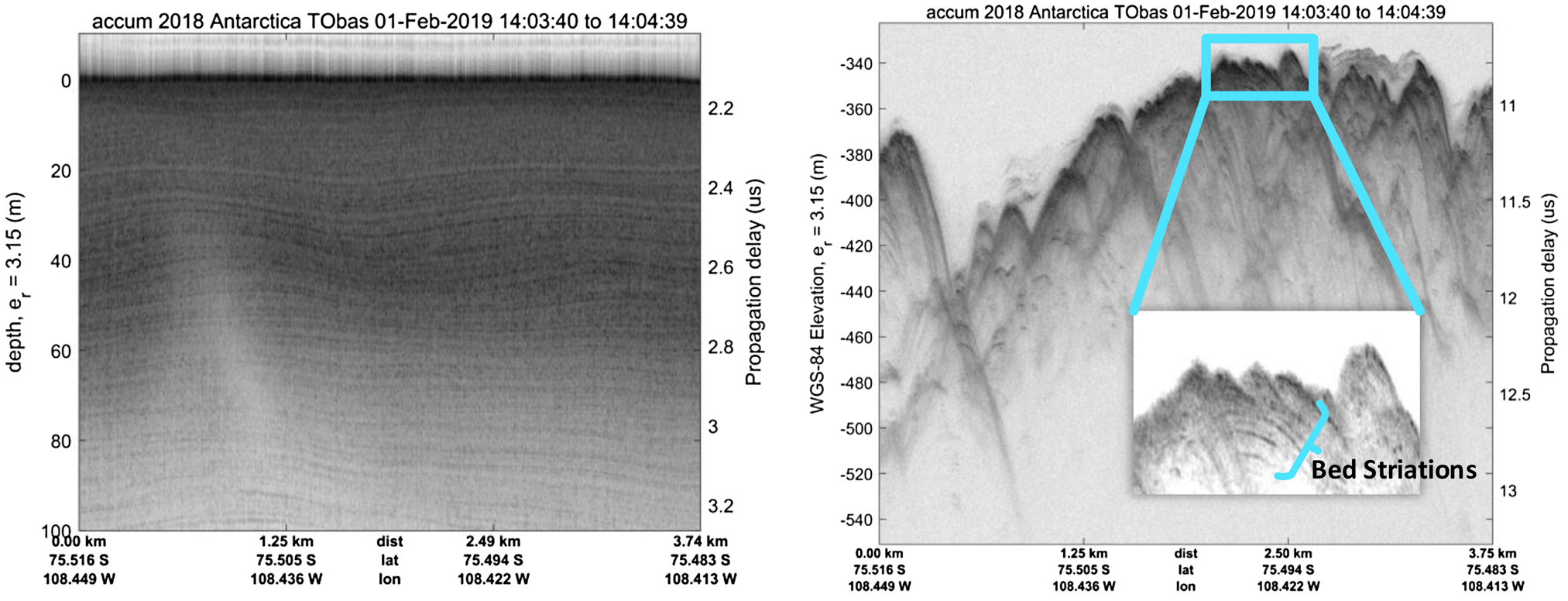
Fig. 8. Magnified surface (left) and bed (right) of the Accumulation-C echogram in Figure 7. The surface image shows good layering as well as return power contrasts that correlate to density variations. The bed image includes a region of striations in the bed. Note that the contrast and brightness of the inset image have been modified to help make the striations visible (Paden and others, Reference Paden2019).
4. Snow radar
Table 4 provides an overview of the snow radar. The original snow radar was designed for the measurements of snow cover on sea ice and operated over the 2–8 GHz band (Panzer and others, Reference Panzer2013). The upgraded 2–8 GHz snow radar now operates over 2–18 GHz (Rodriguez-Morales and others, Reference Rodriguez-Morales, Leuschen, Carabajal, Wolf and Garrison2018; Rodriguez-Morales and others, Reference Rodriguez-Morales2019) and has been used to collect terrestrial snow cover over land (Li and others, Reference Li2019b).
Table 4. Summary of snow radar configurations

a System was integrated; however, vehicle was lost prior to mission.
b System developed and integrated, but has not deployed yet.
4.1 UWB snow
The UWB snow radar has flown on NASA's P-3 and NASA's DC-8 as part of OIB since 2017 (Rodriguez-Morales and others, Reference Rodriguez-Morales, Leuschen, Carabajal, Wolf and Garrison2018). It combines and extends the capabilities of 2–8 and 12–18 GHz (Ku radar discussed in the next section) radars previously flown for OIB. Figure 9 shows an echogram from this deployment (Rodriguez-Morales and others, Reference Rodriguez-Morales2019). The inset image shows that the radar is capable of detecting snow depths as small as 3 cm. We also performed a high-altitude operation feasibility study for integrating the UWB onto the NASA Global Hawk (Talasila, Reference Talasila2014). As part of this work, a snow radar SAR image processor was developed, as well as deconvolution methods to further reduce range sidelobes. Finally, a miniaturized version of this radar was developed (UWB Snow Mini) for integration onto the Vapor 55 helicopter UAS (Kaundinya and others, Reference Kaundinya, Rodriguez-Morales, Arnold and Patil2018).

Fig. 9. Example of UWB snow radar echogram from the 2017 deployment. As the image shows, the instrument has a centimeter-scale vertical resolution (Rodriguez-Morales and others, Reference Rodriguez-Morales2019).
4.2 Snow-C
A compact version of the snow radar was originally developed in 2013 for operation from NASA's SIERRA UAS. The system was integrated and ground tested, but never flown as the vehicle was lost prior to the mission beginning (Maslanik, Reference Maslanik2013). In 2018, the Snow-C flew for the first time on a Single Otter (SO) aircraft in Alaska as part of OIB (Li and others, Reference Li2019a). During these flights, snow radar data were collected over snow-covered mountain summits, icefields and glaciers including the summits of the Wrangell and Bona mountains, the Bagley icefields and multiple glaciers. The echogram on the left side of Figure 10 was collected over Walsh Glacier and shows seasonal snow thickness and crevasses at the snow–ice interface. The echogram on the right of Figure 10 was collected over Chisana glacier and shows multi-year snow layers.

Fig. 10. Measured seasonal snow depth over Walsh Glacier (left), and radar echogram showing multiple snow layers over Chisana Glacier (right) (Li and others, Reference Li2019a). These data were collected using the Snow-C installed on the Single Otter.
5. Radar altimeters
Table 5 is an overview of the CReSIS radar altimeters, which includes the Ku band radar and the Ka band radar. As mentioned in the previous section, the Ku band operation is covered by the UWB snow radar.
Table 5. Summary of radar altimeter configurations

The Ka radar was developed for improved surface topography measurements. This system operates with an add-on ‘mini-module’ consisting of the radio frequency subsection electronics, while the snow radar digital system drives the Ka radar. A similar system has also recently been developed for the Ku radar. The Ka-Mini Module was first flown on the NASA C-130 in 2015 as part of OIB. Figure 11 shows an echogram from a region with dry snow. Despite the high frequency of operation, the snow–firn interface is visible at a depth of ~2 m (Li and others, Reference Li2019b).

Fig. 11. Echogram over dry snow from the Ka Radar installed on the C-130. The snow–firn layer is apparent at ~2 m below the surface.
6. Next-generation polar remote-sensing platforms
With the miniaturization of many of the radar systems, polar remote sensing using small UAS is now realizable. The CReSIS G1X is a 38.5 kg fixed-wing UAS used for the first successful sounding of ice with a radar from a UAS (Leuschen and others, Reference Leuschen2014). This vehicle represents the first-generation of small UAS that CReSIS has developed for remote-sensing applications.
Our experience in developing autonomous platforms and sensors suggests that the most viable path for widespread UAS operation by non-engineers and/or novice pilots is to enable low-speed, low-altitude, lightweight air vehicles with increased autonomy – particularly multi-rotor platforms with the ability to hover. With this in mind, the next-generation remote-sensing platforms we are developing include vehicles with vertical takeoff and landing (VTOL) capabilities (Fig. 12). This vehicle configuration offers the ideal compromise between payload capacity, range capability and vehicle complexity. The VTOL capability of the vehicle will significantly reduce the complexity and logistics of operating the vehicle at remote field locations by eliminating the need for a runway, as well as the highly specialized operator skills to conduct fixed-wing takeoff and landing. The fixed-wing mission operations will result in advantageous performance (>4 h endurance) compared to standard VTOL rotorcraft. We are currently modifying and flight testing several fixed-wing UAS with electric motors, so they can perform VTOL, and expect the first deployment of these vehicles in 2020.

Fig. 12. Fixed-wing VTOL platform with integrated antennas.
7. Future work
In addition to developing our own small customizable UAS, we have also integrated our radar systems onto a small UAS helicopter. Figure 13 shows the UWB Snow Mini radar integrated onto AeroVironment's Vapor 55 UAS. While the fixed-wing VTOL UAS in Figure 12 can takeoff vertically, it still has very limited hovering capabilities. The low-flying and hovering capabilities of the helicopter can increase the signal-to-noise ratio in particularly difficult spots by pushing clutter angles outside the field of view and increasing integration time.

Fig. 13. UWB Snow Mini integrated on the Vapor 55 UAS helicopter.
We are also working on multi-pass processing for the RDS systems. An initial assessment of multi-pass processing using repeat flight lines over Russell Glacier with the HF Sounder Mini in 2013 showed good phase coherence of the surface and the bed returns with only small variance ~0° (Arnold and others, Reference Arnold2018). This initial feasibility assessment has expanded with the addition of MCoRDS data collected from 2011 to 2014 for multi-pass tomographic processing and cross-track slope estimation of specular internal layers. Using the multi-pass processing approach, two combined sets of 15 channels obtained very accurate estimates of the cross-track slope (within ±0.05°) (Miller and others, Reference Miller2019a). By co-registering these images and applying corrections based on the estimated cross-track slope, multi-pass differential SAR was used to show the downward movement of layers over three consecutive years (Miller and others, Reference Miller2019a). Finally, through array simulations, we have also found that beamforming algorithms used in ice data processing (such as Minimum Variance Distortionless Response) are rather robust to deviations in the ideal multi-pass geometry, but performance does degrade with measurement errors in the vehicle's position and low number of snapshots (<1000) (Miller and others Reference Miller, Randolf, Paden and Arnold2019b). These results suggested advanced beamforming algorithms necessary for clutter rejection could be used in the multi-pass architecture if the data covariance matrix can be estimated with relatively high accuracy.
Additional future work activities include the development of an active radar target to improve system calibration, the development of structurally-integrated antennas to reduce overall system weight on UAS, future miniaturization of radar systems to develop a micro-class of radars weighing <1.15 kg (2.5 lbs) and machine learning for tracking 2-D and 3-D layers.
8. Summary
CReSIS developed a radar suite capable of providing a full vertical profile of the ice column. We recently upgraded these systems with two primary focuses: increasing bandwidth for UWB operations, and miniaturizing systems to improve integration flexibility. These upgrades have led to improved measurement resolution, internal layer tracking, bed detection and the ability to perform radar sounding from a small UAS. The focus for next-generation remote-sensing platform development will be on small UASs with VTOL capability. The motivation for this is to eliminate the need for runways (thus improving field deployment capabilities) and increase access to such technology for small science teams.
Acknowledgements
The National Science Foundation (NSF) Grant ANT-1229716 supported the development and deployment of the UWB RDS and UWB Snow Radar. The Paul G Allen Family Foundation and NSF ANT-0424589 supported the development and deployment of the HF Sounder Mini, while the high-power version of the HF Sounder was supported by the KU Endowment Association. Radar development and processing in support of OIB was supported by the National Aeronautics and Space Administration (NASA) NNX10AT68G and NNX16AH54G. The Accumulation-C development and deployment were supported by NSF ANT-1739003. Finally, the UWB Snow Mini radar development was supported by the Kansas EPSCoR program and NASA grant NNX15AK36A. In addition, we also thank our technical support staff and students for their assistance in designing, fabricating, preparing and operating the instruments. This includes Paulette Place, Aaron Paden, Jim Rood, Matt Tener, Hara Talasila, Betty Shang, Teja Karidi and Shravan Kaundinya. Finally, we thank Rachel James for editing this paper and preparing it for final submission.
Author contributions
All authors contributed to this work. E. Arnold is the primary author of the paper and contributed to the aircraft integration of the various sensors and data collection. C. Leuschen contributed to the design and development of the radar systems as well as data collection. F. Rodriguez-Morales contributed to the design and development of the radar systems, aircraft integration and data collection. J. Li contributed to data collection and processing. J. Paden contributed to data collection and processing. R. Hale contributed to the design and development of the antenna fairings and support structures. S. Keshmiri contributed to the development and operation of the G1X-B and data collection.


 Open access