


Introduction
Firn and ice cores collected for climate studies on the Greenland ice sheet tend to be drilled at inland and high-elevation locations where surface conditions remain cold and dry. Drilling sites are chosen to avoid melting that can distort the climate record by redistributing mass and mixing isotopic signals. However, as surface melting on the ice sheet expands (e.g. Fettweis and others, Reference Fettweis, Tedesco, van den Broeke and Ettema2011) and intensifies (e.g. van den Broeke and others, Reference van den Broeke2016), an increasing number of coring studies have explicitly targeted the firn column in heavy melt regions to document meltwater processes and melt-driven transformation of the firn column (e.g. Braithwaite and others, Reference Braithwaite, Laternser and Pfeffer1994; Harper and others, Reference Harper, Humphrey, Pfeffer, Brown and Fettweis2012; Machguth and others, Reference Machguth2016; Rennermalm and others, Reference Rennermalm2022). The physical characteristics of these firn cores, such as density and refrozen meltwater (ice content), are compared across space and through time (e.g. Braithwaite and others, Reference Braithwaite, Laternser and Pfeffer1994; Harper and others, Reference Harper, Humphrey, Pfeffer, Brown and Fettweis2012; Machguth and others, Reference Machguth2016; Rennermalm and others, Reference Rennermalm2022). The observations of meltwater retention and densification rates are important for studies of surface mass balance and surface elevation change.
Melt-related processes generate strong heterogeneities in the vertical and horizontal structure of the firn column in Greenland's percolation zone. Densification rate has a seasonal signal owing to the annual cycle of accumulation (Mosley-Thompson and others, Reference Mosley-Thompson2001) and large summer/winter temperature differences (Zwally and Li, Reference Zwally and Li2002). Summer surface melt erases a variable fraction of the youngest snow, leading to an age bias in the annual accumulation. Infiltration of meltwater is highly heterogenous, in both vertical and horizontal directions due to unsaturated flow governed by capillary retention with breakthrough and piping processes (Marsh and Woo, Reference Marsh and Woo1984; Pfeffer and Humphrey, Reference Pfeffer and Humphrey1996). The meltwater refreezes to partially fill grain pores or to create discrete ice layers, irregular ice lenses and vertical ice pipes. The refreezing releases latent heat, which can locally impact densification rate of the remaining firn fraction. The ice content may also alter overburden stresses and vapor flow, further impacting local densification rate. Hereafter, we refer to melt processes as being some or all of the above processes leading to heterogenous firn structure.
Interpreting firn cores from regions where surface melting occurs is challenged by the horizontal and vertical inhomogeneity of melt processes. Differing density profiles and ice structure in closely spaced cores hampers characterization of the densification rate or ice content of a particular site (Xiao and others, Reference Xiao2022). Furthermore, the vertical mass redistribution and the variable densification rate potentially distorts time-equivalent horizons in the layered firn column, further complicating interpretation of a single core or making comparisons between cores. Yet, despite the alterations by melt processes, a firn fraction of the core undergoes progressive densification during burial and aging processes and its density profile should maintain an age–depth relationship.
This study addresses the problem of depth/age distortion in melt-altered firn cores through an analysis of a density dataset from firn cores. We utilize dynamic time warping (e.g. Sakoe and Chiba, Reference Sakoe and Chiba1978), an established time series analysis tool, and a unique array of nine firn cores collected within tens of meters of each other in Greenland's percolation zone. In the absence of inhomogeneous melt processes and highly localized accumulation effects, the age/depth relationship should be near identical across the suite of such closely spaced cores. Dynamic time warping analysis preforms a quantitative assessment of deviations from this condition and attempts to reconcile mismatch. By using this correlation algorithm to identify where firn-density records do not match well, we begin to elucidate complex, inhomogeneous melt processes. Our results quantify the overall differences between cores, reveal that discrepancies partition into discrete depth ranges and allow for an assessment of the age/depth relationship.
Methodology
Experimental core collection at Crawford Point
Nine closely spaced, 10 m long firn cores were collected in the summer of 2007 at Crawford Point, a site located at 1997 m elevation ~175 km to the northeast of Ilulissat (Fig. 1). Average annual accumulation here is on the order of 1 m of snow at ~350 kg m−3. During the prior 28 summers, the site experienced an average of 13 d with surface melt, although melt days ranged from 0 to 48 d (Brown and others, Reference Brown, Harper, Pfeffer, Humphrey and Bradford2011). The firn temperature at 10 m depth was not significantly altered from the mean annual air temperature implying latent heat release by refreezing was minimal relative to the lower percolation zone (Humphrey and others, Reference Humphrey, Harper and Pfeffer2012). This dataset is therefore representative of the upper reaches percolation zone where melt processes alter the firn column, but on the relatively low end of the spectrum.

Figure 1. (a) Density profiles of Crawford Point sites G1–G9. The average density profile is shown in red. Black bars indicate solid ice within the core: height of the bar is thickness, and width of the bar indicates the fraction of the ice core occupied by the solid ice (thin horizontal lines extending all the way across the plots indicate ice layers that occupy the whole core cross section). (b) Schematic map indicating the positions of sites G1–G9. (c) Location of Crawford Point in Greenland.
Ice cores were drilled with a Kovacs 9 cm diameter core barrel. Measurements of density and ice content of the cores were conducted in the field (Fig. 1). Many ice layers occupied the entire diameter of the core, but sometimes ice occupied only a portion of the core and the fraction was visually estimated. The weight of core sections was measured to determine density using a calibrated electronic balance with 1 g resolution. Density errors arise from: (a) resolution of weight measurements with the electronic balance (1 g); (b) resolution of length measurements of the core sections (1 cm) and (c) in some cases, irregular core breakage leading to length/volume errors (variable, but in rare cases up to 5 cm broken at 50% volume). Due to the variability of the length of retrieved core, no single number is representative of measurement error. We thus adopt a general uncertainty of density measurements ±5%; errors above this are believed to be rare and errors below this most common.
Firn-density estimation and resolution downscaling
We estimate firn-density and downscale-density measurements to centimeter spacing in three steps (Supplementary Fig. 1). Bulk-density values are determined by weighing intervals of core that include both firn and ice. Because we are interested in the impact of unpredictable and heterogeneous ice formation on ice core records, we sought to remove these ice layers and focus analyses on the firn records. We estimated firn-density values through a weighted average approach, estimating the density of the firn fraction based on the originally reported bulk-density measurements and the reported ice fraction (Harper and others, Reference Harper, Humphrey, Pfeffer, Brown and Fettweis2012). Second, we removed all layers consisting of 90% or more ice. Lastly, we linearly interpolated between the estimated firn-density values to generate a centimeter-resolution firn-density record for each of the nine (G1–G9) sites (e.g. see Supplementary Fig. 1). Note that measurements indicate the density of ice formed by infiltration processes averages to 843 kg m−3 due to bubbles and incomplete pore filling (Harper and others, Reference Harper, Humphrey, Pfeffer, Brown and Fettweis2012).
Dynamic time warping routine for ice core synchronization
Dynamic time warping is a time series alignment technique that has been used across disciplines with early applications in speech recognition (Sakoe and Chiba, Reference Sakoe and Chiba1978). Dynamic time warping has been applied to geologic time series, with a focus on stratigraphic and paleoclimatic investigations (e.g. Haam and Huybers, Reference Haam and Huybers2010; Hay and others, Reference Hay, Creveling, Hagen, Maloof and Huybers2019; Ajayi and others, Reference Ajayi2020; Hagen and others, Reference Hagen, Reilly, Stoner and Creveling2020; Baville and others, Reference Baville2022). However, there have also been previous attempts to apply dynamic time warping to ice core records with varying success (e.g. Bay and others, Reference Bay, Rohde, Price and Bramall2010; Schaller and others, Reference Schaller2016; Travassos and others, Reference Travassos, Martins, Potocki and Simões2021). In this study, we employ a publicly available and flexible dynamic time warping algorithm designed specifically for handling time-uncertain stratigraphic times-series data (Hay and others, Reference Hay, Creveling, Hagen, Maloof and Huybers2019; Hagen, Reference Hagen2023).
All dynamic time warping approaches involve constructing an n × m cost matrix filled with the squared residuals of every possible point pairing between the two time-series datasets (of lengths n and m, respectively; squared difference matrix; see Fig. 2). One of these time series must be designated as the target record, serving as an alignment ‘scaffold’ without modification by the dynamic time warping algorithm, while the y (or time) axis of the other time series (termed the candidate record) is stretched and/or squeezed (thereby ‘warping’ the time axis; depending on the most optimal path through the cost matrix) to best fit the target record. The algorithm variant made available by Hay and others (Reference Hay, Creveling, Hagen, Maloof and Huybers2019) adds two geologically relevant penalty functions, controlled by the g and edge parameters (see Fig. 2), that modify the cost matrix according to accumulation rate and temporal overlap. The algorithm multiplies the outside edges of the squared difference matrix by the edge parameter value. The algorithm then computes the cumulative difference matrix, multiplying any off-diagonal values by some factor of the g parameter value, depending on its relative position. The algorithm determines the alignment path through this cumulative difference matrix by charting the route that accumulates the least cost (or the path of least resistance; see Hay and others (Reference Hay, Creveling, Hagen, Maloof and Huybers2019) for a detailed mathematical description of this dynamic time warping algorithm).

Figure 2. (a) An example dynamic time warping alignment, with the target record (black) plotted along with the aligned candidate record (blue). Vertical lines indicate where the algorithm has inserted a hiatus in the candidate record, while horizontal lines indicate a hiatus insertion in the target record. (b) The cost matrix, filled with the squared residuals of every possible point pairing between the candidate and target records, which are then modified by the edge (edge-modified matrix) and g parameters (cumulative difference matrix). The inset illustrates how the nine upper-right most cost matrix elements are calculated (squared difference in step 1; outside matrix edges multiplied by edge parameter in step 2; eight nearest elements to upper-right most element are multiplied by a factor of the g parameter, according to their relative position). Higher edge parameter values encourage more temporal overlap between the records, while the g parameter value can either encourage or discourage similar accumulation rates between the records (depending on the g parameter value). The algorithm charts the path of least resistance (the accumulation of least ‘cost’; see the blue alignment path in the matrix) through the cost matrix to determine the optimal alignment for the given edge–g value pairing. A perfect 1 : 1 match between the records would instead follow a linear diagonal through the cost matrix (black dashed line). (c) An example of the original candidate record, prior to alignment.
By varying the values of these two parameters (g and edge), a library of potential time-series alignments can be generated, allowing for the exploration of multiple alignments with different stratigraphic implications (see Fig. 2). While this algorithm has been primarily applied to carbon isotope (δ13C) records (Hay and others, Reference Hay, Creveling, Hagen, Maloof and Huybers2019; Ajayi and others, Reference Ajayi2020), it is flexible and can be adapted to other time-series datasets like paleomagnetic secular variation (Hagen and others, Reference Hagen, Reilly, Stoner and Creveling2020) and firn core-density profiles (this study).
In this study, we vary the g and edge parameters across a range of values (0.98–1.01 and 0.01–0.15, respectively, in increments of 0.01). From each library of 60 plausible alignments, we select two solutions to explore: the alignment with the maximum Pearson's correlation coefficient (hereafter the max r alignment), and the alignment that maximizes shared time between the target and candidate datasets (hereafter the max t alignment). In principle, these solutions should be identical if there are little-to-no differences between records, such as the proximal ice core records of Crawford Point. In all site–site alignments, we designate site G9 as the target record because of its representative density profile and its position marginally offset from the other eight sites.
Age–depth modeling for Crawford Point
We constructed baseline depth/age model for Crawford Point using the community firn model (Stevens and others, Reference Stevens2020). The model runs on a daily time step, forced by surface climate data taken from RACMO2.3p2 (Noël and others, Reference Noël2018). We employ the Herron and Langway (Reference Herron and Langway1980) densification scheme, which represents only dry firn compaction processes. The model was initialized with a mean density profile from the ice cores and a measured temperature profile (Humphrey and others, Reference Humphrey, Harper and Pfeffer2012), and then spun-up using the 1961–80 interval repeated over 1000 years. The simulation is simply intended to produce a benchmark case for purposes of offset comparison between different cores, rather than yield the highest fidelity result. As such, no infiltration/refreezing scheme was used so that the age model represents the end member case of no mass redistribution or enhanced densification from meltwater processes.
Results
Assessing density inhomogeneity
Despite their proximity, the Crawford Point-density records do not match particularly well (Fig. 3). Obvious visual differences demonstrate that substantial mass redistribution occurred through melt processes (Fig. 3b). The max r and max t solutions are never identical (Fig. 3b), indicating that the alignment solution that maximizes the amount of shared density values between any two records is not equivalent to the alignment that maximizes the mathematical fit (in terms of the density values). If these sites were virtually identical, the max r and max t solutions would converge and the amount of shared time between the candidate records (G1–G8) and the target record (G9) would approximate 100% (a G9 thickness ratio of 1; see Table 1). While the max t alignments for sites G4–G7 are reasonably close to G9 thickness ratios of 1 (ranging from 0.92 to 1.05; Table 1) sites G1–G3 and G8 differ more substantially (ranging from 0.82 to 1.42; Table 1).

Figure 3. (a) Comparisons between max r (blue) and max t (orange) solutions for density alignments between G1–G8 and G9 (shown in gray). Note the different depth scales for the G2–G9 and G8–G9 alignments, resulting from alignments with lower overlap. (b) The max t composite record (the max t solution for each candidate (G1–G8) alignment with the target record (G9), stacked as a composite record), demonstrating the degree of density heterogeneity across these closely spaced sites. (c) The offset between each max t alignment and the predicted alignment where each firn-density record only reflects compaction and densification processes. The offset between these alignments highlights the impact of melt processes on the depth–depth relationships between these cores.
Table 1. Mean and std dev. of unmatched density value interval thicknesses for each max t alignment (between G1–G8 and G9), as well as the ratio between the max t alignment thickness and G9 total thickness

Ratios <1 indicate that the total max t alignment thickness is less than the G9 thickness.
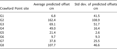
We estimate the offset between the depths assigned by the max t alignments and the predicted depths (assuming that each record is virtually identical with no melt infiltration; Fig. 3b; Table 2). Site G2 has the largest average offset (~162 cm) while site G6 has the smallest (~10 cm), up to ~15% of the ~10 m cores (Table 2). Site G2 also has the most variability in depth offset (std dev. of 108.89 cm) while site G5 is most consistent (std dev. of 2.62 cm).
Table 2. Mean and std dev. of the offsets between the max t alignment (alignments between G1–G8 and G9) the predicted alignment (assuming no melt processes)
Mass redistribution zones
We identify four depth zones across the Crawford Point cores that appear to have a high number of unmatched density values, as determined by the dynamic time warping algorithm: the first is centered at ~100 cm depth, the second occurs between ~200 and 300 cm, the third is centered at ~600 cm and the fourth occurs at ~800–900 cm (Fig. 4a; Supplementary Fig. 2). These are zones where, across multiple sites, the algorithm found it more favorable (in terms of the accumulated cost function) to assign candidate density values to an unconformity (in a stratigraphic sense) than to align them with the target record. Therefore, the algorithm would predict that density values in these zones had been altered (because they cannot be appropriately aligned with the target record) through mass redistribution (mass loss through partial melting and infiltration or mass gain through refreezing in open pore space, which can in turn either enhance or reduce rates of densification within a given length interval). These mass redistribution zones can also be seen in a density variance with depth profile and appear to correspond with ice layer zones identified through our data cleaning (see Fig. 4b; Supplementary Fig. 1). The average size of these intervals of unmatched density values is 24 ± 32.2 cm across all sites (Table 1).
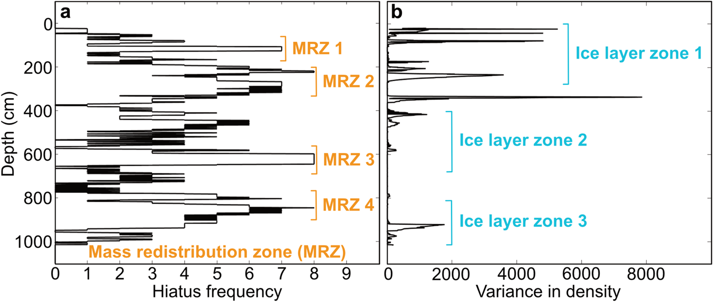
Figure 4. (a) Hiatus frequency over depth, as the dynamic time warping algorithm inserts hiatuses when it is unable to match density values between the candidate (G1–G8) and target (G9) records. A hiatus frequency of 1 means that dynamic time warping algorithm inserted a hiatus in one of the eight candidate records at that depth (while a hiatus frequency of 8 means that hiatuses were inserted in every candidate record at that depth). Higher hiatus frequency may indicate wider spread alteration events (see numbered mass redistribution zones (MRZ) in orange; as opposed to site-specific alteration with lower hiatus frequency). (b) Variance in the max t composite firn-density composite record across depth and all nine sites. Variance is highest in the upper 400 cm, declining with depth. This trend likely reflects both alteration and compaction processes, where firn density near the surface is more likely to be altered by infiltrating meltwater and less impacted by compaction due to less overlying firn. Ice layer zones, identified through data cleaning protocols, are indicated in cyan and appear to be potentially correlative with higher firn-density variance and the interpreted mass redistribution zones in (a), suggesting that melt processes may be responsible.
Impact on percolation zone age–depth relationships
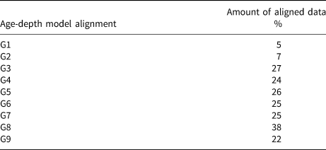
We also used the dynamic time warping algorithm to align each Crawford Point site with an age model to understand the impact of melt processes on core age–depth relationships (using the age model as the alignment target in every case; Figs 5, 6). The age model only takes dry snow densification into account, so any mismatches should be an indication of the impact of melt processes on the age–depth relationships. For the Crawford Point site alignments with the age model, we normalized the density values because alignments with the absolute values were not at all realistic, which is already an indication of the pervasive impact of melt processes on the age–depth relationship. After conducting the normalized alignments (Fig. 5), we tabulated the amount of density values (in %) from each core that are aligned with the age model (Table 3). Most of the sites have roughly a quarter of their density values aligned with the age model, with the exceptions of sites G1 and G2 with <10% alignment each and site G8 with ~38% alignment (Table 3). Note that we do not have independent age control for these sites, so this is not a measure of how accurate the age–depth relationship is, but instead a measure of the proportion of the reported density signal that can be aligned with the predicted density signal (of the age model) that assumes no melt processes.

Figure 5. (a) Max t alignments between each Crawford Point site (G1–G9, shown in blue; the candidate records) and the firn-density age–depth model (shown in gray; the target record). Firn density was normalized prior to alignment to achieve more realistic alignments (alignments using absolute firn-density values found very little overlap). In every case, the max t alignments suggest that a portion of the uppermost Crawford Point site firn-density stratigraphy cannot be aligned with the uppermost portion of the age–depth model. These failures indicate possible alteration to the upper portion of the Crawford Point firn-density records. Note that gray-dashed lines indicate the top and bottom of the firn-density age–depth model, as it is often obscured by the aligned Crawford Point site stratigraphy in the plots. (b) The firn-density age–depth model for Crawford Point. In (a), ~75% of the Crawford Point site firn-density values cannot be matched with the firn-density age–depth model.
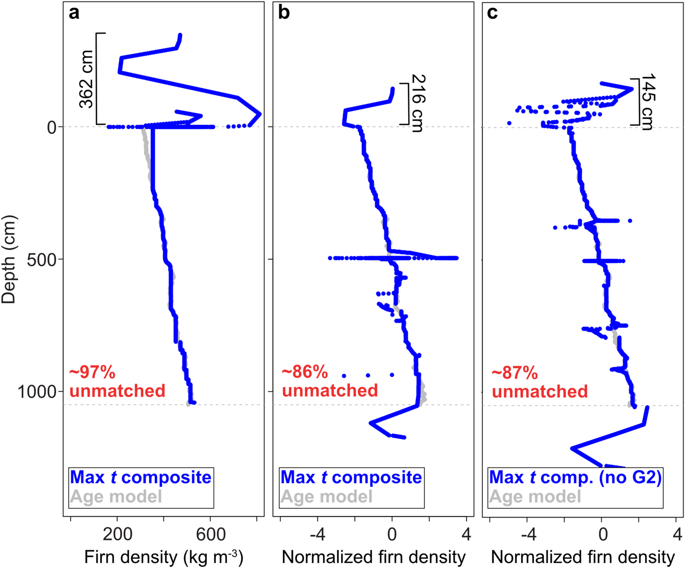
Figure 6. (a) Max t alignment solution between the max t composite record and the firn-density age–depth model, using absolute density values. (b) The max t alignment solution between the max t composite record and the firn-density age–depth model, using normalized density values. (c) The max t alignment solution between an altered max t composite record (excludes the Crawford Point site G2 because it differs so greatly from the other sites) and the firn-density age–depth model, using absolute density values. Like the individual Crawford Point site alignments with the firn-density age–depth model, the max t composite alignments suggest that a portion of the uppermost Crawford Point firn-density stratigraphy cannot be matched with the firn-density age–depth model (the amount of overlying stratigraphy is indicated in black in (a–c)). In (a–c), ~86–97% of the Crawford Point firn-density values cannot be matched with the firn-density age–depth model. Note that gray-dashed lines in (a–c) indicate the top and bottom of the firn-density age–depth model, as it is often obscured by the aligned Crawford Point site stratigraphy in the plots.
Table 3. Amount of firn-density values (in %) successfully aligned with the firn-density age–depth model for each Crawford Point site
Lastly, we aligned the max t composite (Fig. 3b) with the age model (using the age model as the alignment target) to see if greater data density (with respect to the individual cores) improved the alignments. We found similarities between the composite alignment and the individual alignments, where the normalized data resulted in a better alignment and a large proportion of the signal remained unmatched with the age model (Fig. 6). We tried removing site G2 from the composite record, as its alignment differs the most from expectations (see Fig. 3 and Table 2), but this did not have a strong impact on the resulting alignment.
For every alignment with the age model, we found that a portion of the uppermost stratigraphy is aligned above the top of the age model. While the placement of these values is not stratigraphically possible (because the top of the age model represents the surface), this indicates that these density values have been altered beyond alignment (even when normalized) with the age model, likely due to surface and melt processes. The thickness of these overlying values varies by site (Table 4), with the smallest resulting from the alignment of the max t composite (excluding G2) with the age model (145 cm) and the largest from the G4–age model alignment (376 cm) (Table 4).
Table 4. Amount of overlying stratigraphy for each max t alignment with the firn-density age–depth model
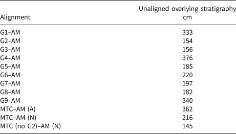
AM, age model; MTC, max t composite; A, absolute density values; N, normalized density values; no G2, data from site G2 excluded.
Discussion
Through dynamic time warping analyses, we demonstrate that melt processes substantially impact firn-density profiles, distorting age–depth relationships at a relatively low-melt region of the percolation zone. There is no obvious spatial reason for the resulting core depth offset trends, as site G6 is the closest site to G2 in the Crawford Point grid (~3 m away) and both are similarly distal from site G9 (~50 m away; the target record). This demonstrates the heterogeneity and localized nature of the impact of melt processes on ice core-density records.
Site G2 differs substantially from sites G1 and G3–G9 (Fig. 1), leading to poor alignments with G9 and the age model (Figs 3, 5). Because the G2-density profile does not monotonically increase with depth (see the large drop in density values below 300 kg m−3 at ~5 m; Fig. 1), it is difficult for the algorithm to accurately align G2 with G9 or the age model, leading to a large portion of G2 assigned above or below the G9 and age model density profiles (see Fig. 5). For this reason, we tried removing G2 from the max t composite when aligning with the age model (Fig. 6). Note that depth assignments for values above and below the target data are estimated based on accumulation rate implied by the aligned values and should not be interpreted as true depth.
Variable accumulation across the small study plot is unlikely to have played a significant role in generating the variability between cores. Detailed studies at the East Greenland Ice Core Project (EastGRIP) site (Zuhr and others, Reference Zuhr, Münch, Steen-Larsen, Hörhold and Laepple2021) show that erosion/deposition processes tend to flatten small surface roughness features over time, a phenomena we have also observed in our study region. These processes may generate small spatial variability in the initial snow density, but this would likely average out quickly during firn densification.
The identified mass redistribution zones are likely driven by melt processes, as the reported density values are higher than expected if driven solely by densification processes (Figs 5, 6). We would predict that some of these zones may align with easily observable ice layers in the cores, resulting from meltwater refreezing and amplifying density values. Indeed, noted ice layers in these sections do fall into three zones: an upper zone between ~0 and 300 cm (ice layer zone 1 in Fig. 4b); a middle zone between ~400 and 750 cm (ice layer zone 2 in Fig. 4b) and a lower zone between ~800 and 1000 cm (ice layer zone 3 in Fig. 4b). Only using the ice layers to identify mass redistribution zones would provide a coarser view of the influence of melt processes, only focusing on obvious ice layers and missing firn mass amplification. However, the presence of these ice layers within the mass redistribution zones that we identify with the dynamic time warping algorithm is a good ground-truth test that the algorithm is indeed identifying the influence of meltwater processes. Because these zones are regional (identified across multiple sites; Fig. 4), at least at the scale of Crawford Point, larger melting events are likely driving the mass redistribution. However, more localized, heterogeneous point-to-point variability between sites (e.g. see Fig. 3b) highlights the heterogeneity in (and difficulty in predicting) melt processes.
Alignments with the age model indicate that the overall shape of the density profiles retain some information about the age–depth relationships (the normalized alignments), while the absolute density values themselves are not reliable for synchronization. The thicknesses of overlying stratigraphy (Table 4) could be used as an estimate of the penetration depth of surface melting in each core, where the density values have been altered beyond alignment with the age model.
Near the lowest elevations of the percolation zone where ice layers are numerous and can be decimeters-to-meters thick, the age/depth relationship should be strongly distorted by melt processes. Crawford Point, however, is located at 2000 m elevation where prior to the collection of these cores, relatively low-intensity melting occurred for just under 2 weeks of the year on average (Brown and others, Reference Brown2012). Our grid of cores demonstrates, however, that large discrepancies exist between cores. Dynamic time warping analysis of the cores demonstrates distortion of the depth/age relationship, with offsets of up to ~15% over ~10 m.
Nevertheless, a ~100 m paleoclimate ice core was collected <1 km away from our G1–G9 cores during the same year as our drilling (Porter and Mosley-Thompson, Reference Porter and Mosley-Thompson2014). Annual boundaries were successfully delineated in the core based on distinct seasonal high/low swings of isotope values (Porter and Mosley-Thompson, Reference Porter and Mosley-Thompson2014). This suggests an inconsistency: our analysis shows that based on density and ice content profiles, closely spaced cores are strongly and variably distorted, but Porter and Mosley-Thompson (Reference Porter and Mosley-Thompson2014) delineated obvious time horizons based on isotope profiles. The implied explanation is that melt processes at this site redistribute mass within and between years such that the thickness of layers can be distorted, but layer boundaries between years remains identifiable based on the very strong seasonal swings in isotope values.
Conclusions
Our study shows that dynamic time warping may be a useful tool for identifying heterogeneous zones of mass redistribution and constraining the impact of melt processes on firn-density profiles. This is particularly relevant to the growing number of studies targeting cores in the Greenland percolation zone. First, we find that melt processes substantially alter the density profiles of the ~10 m cores from Crawford Point, inhibiting confident synchronization of these records and requiring vertical stretching and compression of, on average, <1 to ~16% of the core lengths to achieve optimal alignments. Second, we identify mass redistributions that appear to coincide with ice layers but also represent more heterogeneous melt processes that would be missed if only ice layers were considered (e.g. mass amplification through meltwater refreezing in open underlying pore space). Third, melt-driven density alterations are so severe that they inhibit age model assignments, where ~75% of the density measurements from each core cannot be matched with the example age model-derived density profile (said differently, only ~25% of the firn fraction demonstrates reasonable age–depth relationships; see Fig. 6). Understanding age–depth relationships in firn-density records is key to climate forecasting, as near-surface firn is thought to monitor climate (e.g. Braithwaite and others, Reference Braithwaite, Laternser and Pfeffer1994) and firn pore space buffers sea-level rise from meltwater (e.g. Harper and others, Reference Harper, Humphrey, Pfeffer, Brown and Fettweis2012). Our study seeks to constrain the extent and influence of melt processes on firn-density profiles for the first time, both in terms of core-core synchronization and age model alignment. Future research should extend this analysis scheme beyond the hyper-localized core collection of Crawford Point to assess the influence of melt processes on ice cores across the Greenland percolation zone, particularly at lower elevations where melting is more intense.
Supplementary material
The supplementary material for this article can be found at https://doi.org/10.1017/aog.2023.52.
Acknowledgements
Hagen acknowledges support from the Agouron Institute Geobiology Postdoctoral Fellowship program and Princeton University. Harper acknowledges support from U.S. National Science Foundation Polar Programs (grants Nos. 2113391 and 1717241). We thank editors D. MacAyeal and T. Jóhannesson, as well as two anonymous reviewers for their constructive feedback that greatly improved this manuscript. Invaluable guidance and support were provided by J. Creveling, A. Maloof and E. Trower.


 Open access