1. Introduction

The practical interest in a numerical model of pack ice generally comes about because of its forecasting potential for marine transportation and other offshore activities such as hydrocarbon exploration. The development of such a model also provides a very useful focus for planning an integrated field program in an area such as the seasonal sea-ice zone of the Labrador Sea (NICOS 1981). Initially, these were the reasons for an ice model for the Labrador Sea, but it quickly became apparent that there was a serious lack of data, both for input and for verification of the model simulations. An historical dataset of surface weather analysis and ice charts are available from the Canadian Atmospheric Environment Service, but no comparable set exists for either surface or geostrophic currents, though there are some references to the general current structure in the Labrador Sea (Reference Gustajtis, LeDrew and GustajtisGustajtis 1979). In recent years some data are becoming available from programs carried out by the Bedford Institute of Oceanography (Reference LazierLazier 1979) and the oil companies (Wright and Berenger unpublished), but these are spot measurements and have limited usefulness for estimating currents over ice-covered portions of the Labrador Sea. The end result is that any disagreement between model results and ice characteristics at the end of the simulation period cannot be confidently ascribed to either the model or the input currents.

In discussions of this problem it became apparent that the best approach might be to assume that the model gives valid simulations and that it is deficiencies in the current data which lead to a lack of agreement with the analyzed data. By varying the currents to get a better fit, a better estimate of the surface currents for the simulation periods may then be obtained. Using the model in this way was first proposed by Dr Uwe Radok. The results of pursuing this suggestion in a systematic way are presented here; however, these results are very dependent on the validity of the model. With the lack of a good current dataset it is only possible to conclude that the model simulations and the estimates of current are reasonable. From the work of Tucker and Hibler (1981) it is probable that the specification of the rheology of the ice affects our estimates of current. Because of this, further studies will use both the model described in this work and one similar to that employed by Tucker and Hibler.

The model used for the simulation is an adaption of that developed for ice forecasting in the Bay and Gulf of Bothnia (Udin and Ullerstig 1977). The major changes were the use of a Labrador Sea grid and the inclusion of the effect of non-zero currents.

This work presents the results of a simulation for one week in February 1977 when there was a certain amount of data on ice drift available (LeDrew and Culshaw 1977) as well as the normal sources of data. Previous simulations presented results in the form of a comparison between the model results for thickness, concentration, or mass fields and the analyzed data (Denner and Keliher 1981). The latest simulation added a comparison between model ice drifts and actual drift (Foley and Keliher unpublished). Here, only comparisons of the latter sort will be presented.

Model results are presented for three regimes of currents. These are a long-term averaged or climato-logical set, a slightly modified climatological set, and a set based upon some current meter and ship-drift observations. The best agreement is obtained for the modified set while the poorest comes from the observations. This latter result seemed very surprising until the ship’s log was checked, and it was found that the satellite navigation was not operational for the early part of the period of simulation when the discrepancy with the climatological dataset was the largest. Using the modified current data, two simulations are presented which show the effect of modifying the Theological specifications of the ice.

2. Model Description

The model is an adaptation of that developed by Udin and Ullerstig (1977). Basically, a momentum balance between air and water stresses, Coriolis force, and ice rheology is combined with a mass equation describing changes in ice thickness and concentration to develop a set of equations describing ice motion. The rheology employed is viscous-plastic: linear viscous when the concentration is less than unity and plastic otherwise. The numerical scheme for the momentum balance is an implicit over-relaxation method while a portioning scheme is used for the mass balance. The first method is Eulerian and the second is quasi-Lagrangian, The two-dimensional grid is approximately 20 km on a side, the time step is six hours and the period of study is seven days.

Input data consists of initial thickness and concentration fields as well as six-hour current fields and geostrophic wind fields. It should be noted that thermodynamic effects and sea-surface tilt are considered negligible.

2(a). Momentum equation

The general equation to compute ice velocity can be written as

(1)

where m represents mass, is the ice velocity, is wind stress at the upper ice surface, is water stress at the lower ice surface, is the Coriolis force and is internal ice stress (rheology).

The calculation of the air and water stresses assumes a logarithmic layer adjacent to the ice and an Ekman layer outside the logarithmic layer. The stresses are then calculated from the gradient of the velocity profile evaluated at the ice surface. Because of the two-dimensional nature of the ice momentum equation, it is convenient to use complex notation to represent the vectors. The ice velocity is written as w = u + iv, while is written as τ_a = τ_ax + iτ_ay, and so on forJeach of the vectors. w_w is the velocity of the current and W_ga the geostrophic wind. The stress terms in complex notation are written as

(2)

and

(3)

where

and

and pj is the density of air, water, or ice, f is the Coriolis parameter, is the coefficient for turbulent viscosity of air or water, X_j is the coefficient for molecular viscosity of air or water, and h_j is the depth of logarithmic layer of air or water.

The Coriolis force is formulated as

(4)

where H is the ice thickness. Internal friction is split into two parts

(5)

where R₁ = α Δ (N τ · w) and represents the viscous part, dominant when the ice is free-floating. To retain the complex notation we define

R₂ is meant to represent the plastic behavior of ice and is assumed to be proportional to the driving force but acting in the opposite direction. It is given by

(6)

where k^* is assumed to be a function of ice thickness and concentration, and is formulated to give the necessary reduction of wind stresses that occur when the ice is heavily concentrated and very thick, as in the original application of the model. For instance k^* = 1 for very close pack of sufficient thickness near the shore. On the other hand, thin ice of high concentrations has a low k^* value, allowing movement. Further discussion is continued in the paper by Udin and Ullerstig (1977). Their formulation has not been changed for this application. The original application of the model did not consider T_W a driving force where R₁ was expressed as -k^*T_a only.

2(b). The mass equation

The general equation for the conservation of mass (vector notation) is:

(7)

where m is the mass, is the ice velocity, and μ is the ice added or removed by freezing or melting.

Ice thickness and concentrations are introduced via

(8)

where pi is the ice density, N is the concentration and H is the thickness. Note that m is mass per unit area and H is average thickness in a grid square. Also N lies between 0 and 1.

Using Equation (8), Equation (7) may be separated into two equations:

(9)

and

(10)

Equation (9) is the thickness balance and Equation(10) is the concentration balance, ψ represents the ice deformation and μ1 + μ2 = μ.

For short time intervals the thermodynamics terms may be neglected. There are now four equations describing the evolution of m, N and H; it is not necessary to solve all four. Equation (9) is dropped and the final set of equations is

(11)

(12)

where

(13)

and

(14)

The model yields time histories of the concentration, mass, thickness, and velocity of the ice. The ice-drift tracks are estimated from the velocities at six-hour time steps.

3. Input Data

The period 8 to 15 February 1977 was selected for this simulation because there was a field program, “Ship-in-the-Ice”, in the Labrador pack ice (LeDrew and Culshaw 1977). Measurements of wind, profiles of ocean currents, and observations of ice characteristics were taken, but, because of various logistic and equipment problems, not all of the data were useful.

The model used initial ice data for the Labrador Sea for 8 February 1977, where most of the data were extracted from the weekly ice charts prepared by the Canadian Atmospheric Environment Service. The concentrations were taken directly from the charts, while thicknesses were calculated as concentration-weighted averages of the various ice types in each grid square. Unfortunately, ice data are not available from the maps north of 56°N. Data for the northern portion of the grid was extrapolated by assuming that the ice characteristics at S6°N simply extended northward more or less parallel to the coast. The data from this procedure roughly agreed with the observations from the ship.

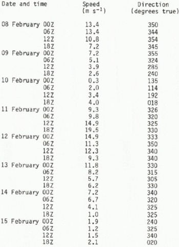
The wind data were taken from both the ship’s observations and the surface weather charts, again produced by the Atmospheric Environment Service. The model uses geostrophic winds so the surface winds, as recorded on the ship, were increased by one-third and turned 30° clockwise. The reverse of this procedure is typically what is used in this area to estimate surface winds from geostrophic values; see Keliher and others (unpublished) for a discussion of this procedure. The map measurements were extracted directly from the maps. These were not considered to be very accurate since there were no meteorological stations within 600 km of the ship and only three or four available for the total model area. The two dataseis were averaged together to provide the final dataset, and Table I shows this data.

Table 1. The Geostrophic Winds Used In The Model

A climatological dataset of currents have been used for previous simulations, and the portion of that dataset in the area of the ship is shown in Figure 1. The data from the field program can also be used for the currents, and this was done in two ways. First of all, drift of the ship can be used if it is assumed that the wind component of the drift is 3% of the wind velocity and is some angle to the rignt of the direction. Based upon the work of Reference LeppärantaLeppäranta (1980) in the Bay of Bothnia, the angle of 20° was used, which is smaller than other workers have used. Once the wind component is subtracted out, the remaining portion is assumed due to current drift. In addition, the current measurements can be used if the motion of the ship is removed; however, it was found that the measurement program was not consistent enough to be of direct use. Instead the first method was used, and, where data were available from the second method, they were averaged with the first. Note that in both cases the accuracy of the data is very dependent on the accuracy of the ship’s navigation. In the early part of the simulation the satellite navigation system was”not operating and navigation by ranging to land targets was used. The drift of the ship was erratic in this early period, and seems to indicate that the ranging was not very accurate. The current dataset as derived from the field program is given in Figure 2,

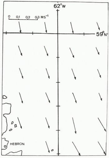
Fig. 1. A vector diagram of the climatological current dataset used in the model in the area of the “Ship-in-the-Ice” program.

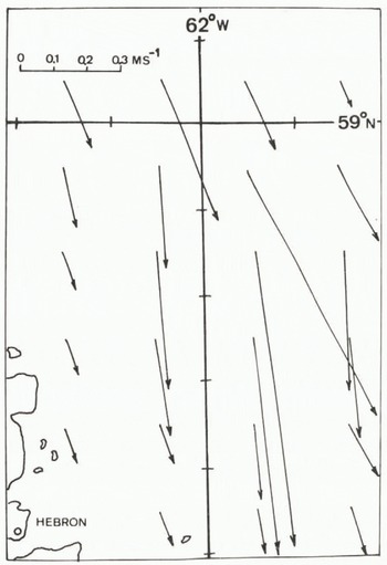
Fig. 2. A vector diagram of the currents estimated from the drift of and observations from the ship.

The most useful data provided by the “Ship-in-the-Ice” program are the ship’s drift. The ship was fast in the ice at this time, and the drift was taken to be representative of the ice in the vicinity.

4. RESULTS

The model produces a time history of mass, concentration, thickness and velocity fields for the ice. Drift tracks are estimated from the ice velocities by noting which grid square contained the drift point. The ice velocity for that grid square is taken as the drift velocity. That velocity multiplied by the time interval gives the drift track for that interval. The sum of interval drift tracks is presented in the figures. Obviously a proper interpolation is preferable and work is underway to make this modification. However, the simpler procedure used here is adequate for present purposes.

Figures 3 to 6 display the ship’s drift, shown as a dashed line, and various modelled drifts, shown as a solid line. Figure 3 has an additional dashed-dotted line which represents the apparent excursions of the track due to navigation problems. The circles represent the position at the start of each day beginning at 00Z on 08 February 1977. Double circles represent locations of no motion between days. The dashes on the latitude and longitude lines are 10’ of latitude by 20’ of longitude which is the dimension of the model grid. The location shown in these figures is on the Saglek Bank just east of northern Labrador. The deserted village of Hebron is indicated.

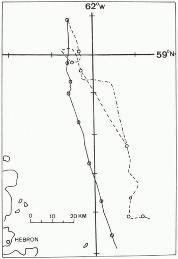
Fig. 3. A comparison of model results (solid line) and ship’s drift (dotted line), the latter being assumed to be characteristic of the local ice drift. The model results are for the climatological currents. The dashed-dotted line is the drift of the ship as indicated by the observations but probably subject to navigational errors. Circles are positions at synoptic hours.

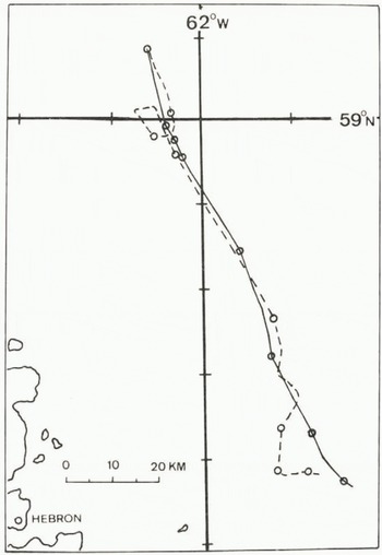
Fig. 4. Similar to Figure 3 except the model results are for the “adjusted” currents.

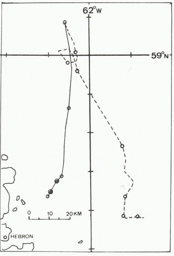
Fig. 5. Similar to Figure 3 except the model results are for the currents of Figure 2.

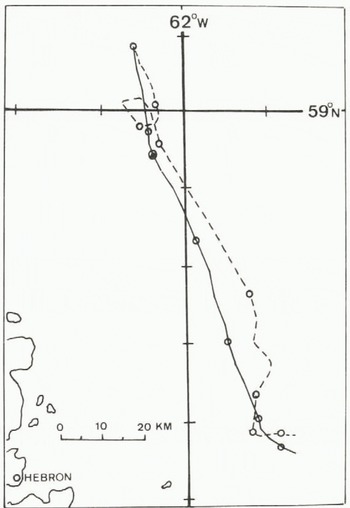
Fig. 6a. Similar to Figure 3 except that the viscous internal friction term has been set to zero (α = 0).

Fig. 6b. Similar to Figure 3 except that k⋆=0.

The results using the climatological current dataset are shown in Figure 3. The loop in the ship’s track is not repeated by the model, but the model drift slows appreciably for this period. The total model drift is to the west of the observed drift, and the final drift points differ by one grid square. This result seems reasonable considering that there has been no adjustment of the data or model parameters.

Figure 4 gives the drift for slightly adjusted currents, which are shown in Figure 7. The modified currents were derived by examining the daily drifts of the ship (that is, the ice drift), noting which grid square the ship was in, and then guessing a new value. The figure shows that this gives quite good agreement with the modelled track being somewhat shorter. As a comparison the drift using the observed currents (Fig.2.) is shown in Figure 5. The modelled drift is quite far to the west, and, during the latter portion of the simulation period, moves into the fast-ice region of the model area. As a result the drift almost ceases. Looking back at Figure 2 it can be seen that the current speeds in the northern part of this figure are quite high compared to either Figures 1 or 7, and, while peak currents as high as this have been observed (Wright and Berenger unpublished), values as large as those indicated in Figure 2 seem unreasonable considering that they are really weekly average values. Thus, the review of the little information that is known about currents in the area, the situation with the field program, and the model simulations indicates that the climatological currents and slightly adjusted current data represent a much better estimate of the actual currents than that displayed in Figure 2.

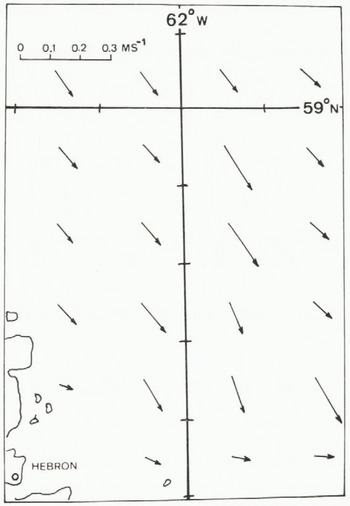
Fig. 7. A vector diagram of the “adjusted” currents which give the results shown in Figure 4.

It would be very tempting to make current estimates on the basis of the simulations alone; however, the assumed rheology of the ice can affect these estimates. Figure 6 displays the results using the adjusted currents for [Equation 33]and α = 0 and k⋆=0 in Equation (5) and Equation (6). Figure 6(a) shows the result for [Equation 36], and there is little change from Figure 4 in this. If we can consider α = 0 to be a “free drift” model, then this could probably be used to estimate currents. Figure 6(b) indicates that k⋆=0 lengthens the drift track significantly and the estimated current values would have been lower if this term had been absent. Figure 6 shows little change in drift direction for the two cases, indicating that the current direction does not depend on a or k^*.

The use of the k^* parameterization was added to the model to reduce the ice velocities in areas of high concentration and fast ice (Udin and Ullerstig 1977). It is not really a proper rheological treatment of any plastic effects, but the results of its inclusion in this model indicates that, while a true free-drift ice model might be useful for a rough estimate of currents, it is necessary to include a proper rheological term. Because of this situation, further model work for the Labrador Sea, and also for the Baffin Bay pack, will use both the model described here and that developed by Hibler (Reference Hibler and ColbeckHibler 1980, Tucker and Hibler 1981).

5. Conclusions

This work has presented some results of numerical modelling of the ice pack in the Labrador Sea. Comparisons were made of drift tracks modelled in a limited area with the only data available for the area which resulted from a field program carried out in February 1977. Thus, the feasibility of using ice-drift data to estimate ocean currents in ice-covered areas was examined. The climatological current used in previous simulations was adjusted to make model drift agree with observed drift and is well within expected currents in the area. However the results depend on assumptions about the rheological or internal friction properties. Hence the study also examined the effects of zero-setting the various terms representing internal friction. The absence of the linear viscous term did not greatly affect the drift tracks, but the absence of the term designed to reduce ice velocities in areas of high concentration changed the drift tracks to a much larger extent. Any “back solved” currents would be affected by the absence of this term.

The “Ship-in-the-Ice” dataset was nearly exhausted with this study so it was not possible to carry out further simulations to study the effect of ice rheology on estimates of current. In order to minimize the uncertainty in the rheological terms, it is planned to apply a numerical model with a better formulation of the rheological terms using the data discussed here.