

INTRODUCTION
It is rather well established that avalanches are a significant contributor to the net accumulation of ice on many glaciers in the high-relief Himalayan mountain range (Benn and Lehmkuhl, Reference Benn and Lehmkuhl2000; Benn and others, Reference Benn, Kirkbride, Owen and Brazier2003; Scherler and others, Reference Scherler, Bookhagen and Strecker2011a; Nagai and others, Reference Nagai, Fujita, Nuimura and Sakai2014). However, the question of quantifying the avalanche accumulation and its long-term variability remains largely unexplored in the literature. If a broader understanding of the mass-balance processes in the Himalaya as well as in other glacierised regions in the world were to be achieved, a technique to address this issue must be developed. Such a development would be of help, on one hand to get a clearer picture of the recent climatic response of the Himalayan glaciers (Cogley, Reference Cogley2011; Scherler and others, Reference Scherler, Bookhagen and Strecker2011b; Kääb and others, Reference Kääb, Berthier, Nuth, Gardelle and Arnaud2012; Gardelle and others, Reference Gardelle, Berthier, Arnaud and Kääb2013) and on the other hand to predict their future evolution reliably (Marzeion and others, Reference Marzeion, Jarosch and Hofer2012; Immerzeel and others, Reference Immerzeel, Pellicciotti and Bierkens2013).
A stochastic and highly localised accumulation of snow and ice on the inaccessible and often hazardous avalanche cones along the valley walls (Fig. 1) makes it difficult to directly measure the avalanche contribution using standard glaciological mass-balance techniques. However, neglecting this contribution would lead to a significant bias in the measurement of the mass balance. Therefore, standard manuals for mass-balance measurement advise against choosing glaciers where a strong avalanche activity is expected (Kaser and others, Reference Kaser, Fountain and Jansson2003). This is a serious limitation as far as Himalayan glaciers are concerned, where avalanche contributions often play a dominant role. For example, Scherler and others (Reference Scherler, Bookhagen and Strecker2011a) have demonstrated that in several regions of the Himalaya the fraction of strongly avalanche-fed glaciers is quite significant. They analyse three characteristic indicators of a strong avalanche activity: (1) high slopes in the ice-catchment area, (2) a high percentage of ice-free catchment above the snowline, and (3) low accumulation area ratio (AAR). Their data from a set of 287 glaciers in the Himalaya and Karakoram show that these characteristics are indeed correlated. In particular, almost all the glaciers with a AAR <0.2 have a very high percentage of ice-free catchment area above the snowline and, thus, are likely to be predominantly avalanche-fed ones. Such glaciers constitute 18% of the all the glaciers studied by them in the Western and South-Central Himalaya. This gives a ball-park estimate that in these regions of the Himalaya: it is likely that a significant percentage of the glaciers (about one in five) are strongly avalanche fed. Several models have been developed to estimate the snow redistribution due to gravitational processes, given the snowfall data and the topography (Gruber, Reference Gruber2007; Bernhardt and Schulz, Reference Bernhardt and Schulz2010). However, a serious lack of reliable snowfall data in the glacierised high Himalaya (Viste and Sorteberg, Reference Viste and Sorteberg2015) limits the applicability of such tools in estimating avalanche contribution to the mass balance of a specific glacier. Moreover the ice-avalanche contribution to the mass balance of reconstituted glaciers (Benn and others, Reference Benn, Kirkbride, Owen and Brazier2003) would not be captured by these methods. This necessitates an alternate indirect method for estimation of avalanche derived accumulation, possibly making use of available glaciological data. We hypothesise that the significant avalanche accumulation exerts dominant control on the observed pattern of shrinkage in these Himalayan glaciers. If so, then this pattern of shrinkage can be utilised to quantify the avalanche contribution.

Fig. 1. (a) The headwall of Hamtah glacier showing large avalanche cones. (b) A massive avalanche rolling down from the Choukhamba massif (7138 m) at the headwall of Satopanth glacier.
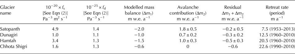
To test this hypothesis, in this paper we first discuss the diagnostic criteria that would allow identification of any strongly avalanche-fed glacier. Then we describe a simple and approximate method to obtain a first-order estimate of the possible avalanche contribution to mass balance using numerical flowline model simulations. The method requires as input the glaciological mass balance and the velocity/thickness profile, long-term retreat and/or thinning-rate data and hypsometric data for the glacier chosen. The flowline model simulations are used to estimate the total accumulation that is consistent with all other available data related to glacier dynamics and glacier geometry. The difference between the modeled and glaciological mass balances, is assumed to be due to avalanche contributions. We cannot rule out various other possible sources of this residual accumulation contribution, e.g. any potential systematic bias in the accumulation measurement due to ill-chosen stake/pit locations or the effect of wind-driven inhomogeneous redistribution of snow and so on. However, we provide other circumstantial evidence drawn from the knowledge of the basin morphology etc. to argue that the estimated missing contribution should be dominantly coming from avalanche feeding. Here, we apply this method for Satopanth (30.73N, 79.32E) and Dunagiri (30.54N, 79.89E; also known as Dronagiri) Glaciers in the Central Himalaya and Hamtah Glacier (32.22N, 77.38E) in the Western Himalaya (Table 1) where strong avalanche activity is suspected, and arrive at first order estimates for the values of the avalanche accumulation. We also perform a control simulation with Chhota Shigri Glacier (32.28 N, 77.58 E), located ~12 km to the west of Hamtah glacier in the western Himalaya, where avalanches are not expected to be an important source of nourishment and thereby check the consistency of our method.
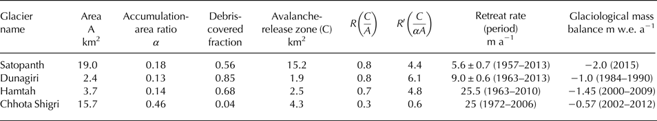
Table 1. Observed glacier properties
IDENTIFYING STRONGLY AVALANCHE-FED GLACIERS
Glaciers with a strong avalanche contribution are usually associated with high and steep head-walls (Benn and others, Reference Benn, Kirkbride, Owen and Brazier2003; Hughes, Reference Hughes2008; Scherler and others, Reference Scherler, Bookhagen and Strecker2011a; Nagai and others, Reference Nagai, Fujita, Nuimura and Sakai2014). Along with the snow and ice, avalanches from the head-wall and the lateral valley-walls bring down debris material to the accumulation zone, eventually leading to the formation of an extensive supraglacial debris mantle at the ablation zone (Benn and others, Reference Benn, Kirkbride, Owen and Brazier2003; Kirkbride and Deline, Reference Kirkbride and Deline2013). The high relief, steep slopes and an abundance of extensively debris-covered glaciers in the Himalaya are thus indicative of a strong avalanche contribution for a significant fraction of them.
Benn and Lehmkuhl (Reference Benn and Lehmkuhl2000) have argued that for any specific glacier, the steady-state AAR value goes down strongly with a relatively high contribution from avalanches to total accumulation as compared to that of the direct snowfall. The large-scale remote sensing data of Scherler and others (Reference Scherler, Bookhagen and Strecker2011a) show that there is indeed a clear correlation of small AAR values with various proxies of strong avalanche activity in the Himalaya-Karakoram, namely, high slopes in the ice-catchment areas, and a high percentage of ice-free catchment above the snowline. Therefore, any glacier that has a very low (<0.2) AAR, but does not show signs of fast retreat or high down-wasting, may be a strongly avalanche-fed one.
Hughes (Reference Hughes2008) has proposed that a high value of the ratio (R) of the total avalanche-release area to the total area of a glacier indicates a strong avalanche contribution on that glacier. He has defined the avalanche-release zone to be the region of the headwall that has slope larger than 30° and is connected to the accumulation zone. However, extensive debris cover that is often associated with strong avalanche activity, suppresses ablation leading to a larger glacier area (Banerjee and Shankar, Reference Banerjee and Shankar2013). This effect reduces the sensitivity of Hughes’ ratio (R) to the presence of avalanche contribution in debris-covered glaciers (Table 1). As an alternative, we use the ratio of the estimated map area of the avalanche-release zone to the map area of the accumulation zone (R′) to identify a significant avalanche activity on any given glacier. This may work better for the debris-covered glaciers since the total accumulation due to the direct solid precipitation (avalanching) is proportional to the area of the accumulation zone (avalanche-release zone) irrespective of the presence of a debris cover. We have estimated R′ to be 4.8, 4.4 and 6.1 on Hamtah, Satopanth and Dunagiri glaciers, respectively (Table 1). These values are, for example, an order of magnitude larger than the corresponding values of 0.6 and 0.9 obtained respectively on Chhota Shigri and Dokriani glaciers – two other Himalayan glaciers with available glaciological mass-balance record from the Western and Central Himalaya. This is a clear pointer towards strong avalanche contributions on Hamtah, Satopanth and Dunagiri glaciers, whereas Dokriani and Chhota Shigri Glaciers may not be receiving any such major avalanche contribution.
Incidentally, out of the set of ~15 glaciers in the Himalaya where glaciological mass-balance data are available, Dunagiri (−1.0 m w.e. a−1) and Hamtah glacier (−1.45 m w.e. a−1) are the ones with the most negative mass-balance values (Vincent and others, Reference Vincent2013). Similarly, as described later, our data from Satopanth glacier for 2015 yields a negative mass balance of −2.0 m w.e. a−1. In Hamtah and Dunagiri Glaciers the details of the accumulation measurement eg, pit locations, total number of pits, etc. are not available. On Satopanth glacier accumulation is not measured directly and is obtained by extrapolation. In spite of possible uncertainty in the accumulation measurements, such large negative values of mass balance, along with above-mentioned morphological characteristics, indicate a strong avalanche activity on these glaciers that may have remained unaccounted for in the glaciological mass-balance estimates.
ESTIMATION OF THE PUTATIVE AVALANCHE CONTRIBUTION
Rationale and method
Our basic postulate is that for any strongly avalanche-fed glacier the glaciological mass balance, which typically does not measure the avalanche contribution, would have a significant negative bias. The glaciological mass balance would then be inconsistent with the observed state and the recent history of the glacier. For example, if the glacier is in a steady state, then the observed steady-state length would be much larger than the length that is consistent with the mass balance. For a retreating glacier, both the long-term retreat rate and the thinning rate may be much smaller than the observed values. It may be noted that since avalanche-fed glaciers are also typically debris covered, they may take a characteristically long time, to show any length retreat even as they lose mass through the thinning of a stagnant tongue after a sharp warming takes place (Banerjee and Shankar, Reference Banerjee and Shankar2013). For such stagnant glaciers, it is important to compare the thinning rates. To observe the discrepancies mentioned above, multi-decadal to century-scale data on thinning and/or retreat are required due to the long response time of such extensively debris-covered glaciers.
Given the above assumption, the avalanche contribution can be estimated by simulating recent evolution of the glacier concerned. Any instantaneous transient state of a glacier in general can be specified by the ice thickness profile for a given bedrock. To arrive at the right transient state, we start with a steady state the length of which is much larger than that of the present transient state and force it with a suitable negative mass balance till a state with reasonable length, velocity and surface profiles are obtained. To make sure that our results are not dependent on the choice of initial steady state, we use more than one initial steady state. Once an approximation of any initial state is constructed, the glacier evolution can subsequently be simulated with the observed mass balance. If this results in a model state that is shrinking much faster than the observed loss rates, it signals the presence of a missing accumulation contribution for the glacier.
In order to estimate the actual magnitude of such a missing term, an arbitrary constant accumulation term is added and is adjusted till the simulated rate of recent thinning and retreat match the observed values. While there may be a complex spatio-temporal pattern of avalanche accumulation on the real glacier, that need not be prescribed in detail for a reasonable fit to the observed glacier-averaged shrinkage rates as long as the net avalanche accumulation is captured correctly. This is due to the strongly diffusive nature of ice flow, which smooths out any observable effects of such variability on the glacier dynamics. This also implies that our method would only allow estimation of long-term mean values of the magnitude of the avalanche contribution, as the diffusive ice-dynamics filters out the details of the short wavelength and high frequency spatio-temporal variability of the contribution.
The flowline model
The method discussed above can be implemented using a simple 1-D flowline model of glacier dynamics. A flowline model describes the time evolution of the thickness profile, h(x, t), of a glacier along the central flowline parametrised by the distance x [e.g., Banerjee and Shankar (Reference Banerjee and Shankar2013)] as,
 $$\displaystyle{{\partial h} \over {\partial t}} = - \displaystyle{1 \over w}\displaystyle{{\partial} \over {\partial x}}(whu) + \dot b,$$
where w(x) is the width of the glacier at the point x, u(x, t) the vertically averaged velocity and $\dot b(x,t)$
the point annual mass-balance rate in ice-equivalent unit. Note that throughout this paper we use ‘mass balance’ to designate mass-balance rates with units m w.e. a
−1. Also, the water-equivalent rates as used otherwise in this paper can easily be recovered from ice-equivalents (Cogley and others, Reference Cogley2011). The ice velocity is related to the ice thickness through a constitutive relation derived under the shallow-ice approximation,
$\dot b(x,t)$
the point annual mass-balance rate in ice-equivalent unit. Note that throughout this paper we use ‘mass balance’ to designate mass-balance rates with units m w.e. a
−1. Also, the water-equivalent rates as used otherwise in this paper can easily be recovered from ice-equivalents (Cogley and others, Reference Cogley2011). The ice velocity is related to the ice thickness through a constitutive relation derived under the shallow-ice approximation,
 $$u = \left( {\rho gh( - s + \displaystyle{{\partial h} \over {\partial x}})} \right)^3\left( {\displaystyle{{\,f_{\rm s}} \over h} + f_{\rm d}h} \right).$$
ρ is the ice density and g is the acceleration due to gravity and s the bedrock slope. f s and f d are parameters controlling the sliding and deformation contributions to the total flow. Oerlemans (Reference Oerlemans2001) has suggested a value of 5.7 × 10⁻²⁰ Pa−3 m2 s−1 and 1.9 × 10⁻²⁴ Pa−3 s−1 for f s and f d, respectively. However, the f s and f d values are typically used as a tuning parameters of the model (Adhikari and Huybrechts, Reference Adhikari and Huybrechts2009). The values used in modelling various glaciers in the Himalaya are in the range 0.19 − 1.75 × 10⁻²⁰ Pa−3 m2 s−1 for f s, and 1.7 − 5.3 × 10⁻²⁵ Pa−3 s−1 for f d (Adhikari and Huybrechts, Reference Adhikari and Huybrechts2009; Venkatesh and others, Reference Venkatesh, Kulkarni and Srinivasan2012; Banerjee and Shankar, Reference Banerjee and Shankar2013; Banerjee and Azam, Reference Banerjee and Azam2016). Starting with an initial thickness distribution, if the mass-balance profile as a function of time are known, then Eqn (2) can be used to find out h(x, t) at all subsequent time t for any given bedrock geometry and width distribution. If the mass balance does not vary with time then the glacier reaches a corresponding unique steady-state profile after a characteristic time, independent of the input initial thickness profile.
Implementation
We start with the surface-elevation profile along the central flowline and the mass-balance profile of the glacier concerned. Depending on the surface-elevation profile, we pick a piece-wise linear bedrock with two to three segments. We assign a width for each grid point on the bedrock, so that the bedrock has the same area-elevation distribution as the present glacier. We then simulate the glacier with a range of values of avalanche contribution added around the top of the glacier, such that corresponding steady-state lengths are longer than present glacier length. Subsequently, we simulate the glacier as the avalanche term reduces at a constant rate and store the intermediate transient states. The experiment is repeated for several values of the above rate of reduction. Then we plot data for all the intermediate states along with the corresponding observed data, and search for the right set of states so that the initial glacier surface-elevation and/or velocity profiles, glacier length, approximately match the observed data that is available for that glacier. The chosen transient state initial state is then evolved with the avalanche term fixed at its initial value. At this stage, we also tune the constant flow parameters f s and f d within reasonable limits, to the surface-velocity and thickness profile, retreat rate and net balance of the simulated state so that a reasonable match with the corresponding observed data is achieved (see Figs 4–6). If a good match is not found at this stage, we change the bedrock profile and repeat the whole procedure. While the actual glacier geometry might be more complex and there could be complications of tributaries etc., in the end our initial configuration has similar length, area-elevation distribution and a similar central-line velocity profile compared to the real glacier. This should ensure a similar dynamical behaviour in both the simulated and the real glaciers. We refer to the above numerical procedure as experiment (1). Subsequently, we perform another experiment, experiment (2). Here, the initial transient profile, as obtained above, is forced only with the glaciological mass-balance profile, with the constant avalanche term turned off, to see if it is consistent with observed recent dynamics of the glacier. Depending on the available data, we run these experiments for up to 50 years or more.
Given the approximate nature of our method and the uncertainty implicit in the input data, we tune the parameters by trial and error to produce a reasonable match with the observed data to the eye. In view of the large uncertainties of the data used, we decided not to apply a systematic fitting procedure here and limited ourselves to explore the sensitivity of our results to various tunable model parameters and the choice of the initial state. These details are described in the Results and Discussions section.
Satopanth glacier
For Satopanth Glacier (Fig. 2a), a front-averaged retreat rate of 5.6 ± 0.7 m a−1 during 1957–2013, and a thinning rate of 0.18 ± 0.22 m a−1 on the lower ablation zone during 1962–2013 has been reported (Nainwal and others, Reference Nainwal, Banerjee, Shankar, Semwal and Sharma2016). The mean velocity profile for the period 2000–07, as obtained from remote-sensing data (Scherler and others, Reference Scherler, Bookhagen and Strecker2011a), and the surface-profile data for the year 2000 from Shuttle Radar Topographic Mission (SRTM1) DEM (Farr and others, Reference Farr2007) are used.
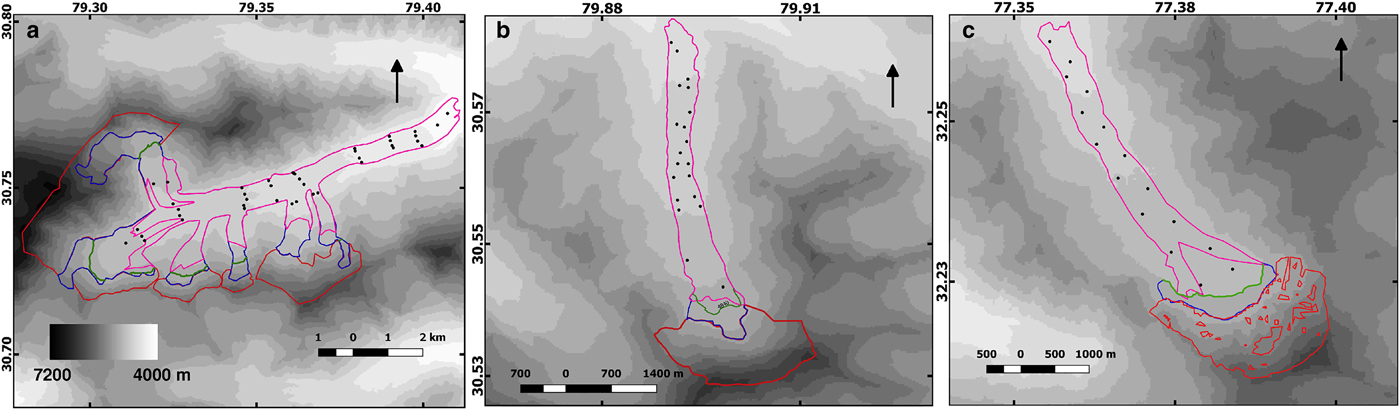
Fig. 2. Maps showing glacier boundary (blue), the extent debris cover (pink), potential avalanche release zone (red) for (a) Satopanth glacier, (b) Dunagiri glacier and (c) Hamtah glacier. The background is the 200 m grey-scale contour map of SRTM1 DEM. The corresponding ELAs are shown as green lines. Approximate stake locations are shown as black dots.
The mass-balance measurement for this glacier has been initiated by our group during 2014 and the results would be reported in detail in a separate publication in the future. Here, we use our preliminary data for the mass-balance year October 2014 to October 2015 that is derived from 40 stakes distributed over an elevation range of 3950–4625 m on the accessible stretches of the glacier (Fig. 2a). From the stake data, two best-fit elevation-dependent linear mass-balance profiles are extracted – one each for the debris-covered and the debris-free ice, respectively. For the inaccessible debris-free part at the higher reaches of the glacier where no stake data is available, the mass-balance values are extrapolated using the above linear profile with an upper cut-off of 1.5 m w.e. a−1 applied to the accumulation values. To compute the mass balance in each elevation band, we use the sum of the two mass-balance values weighted by the corresponding debris-covered and debris-free ice fraction at that elevation band (Fig. 3). The equilibrium line altitude (ELA) of 4910 m obtained from the extrapolation of the linear mass-balance profile for the debris-free ice compares well with the independent estimate of 4840 m from the highest position of the end-of-summer transient snowline elevation as observed in cloud-free Landsat scenes from the year 2013 and 2016. To model the glacier during experiment (1), the added avalanche is spread uniformly over the region within the elevation band 5425–4600 m.
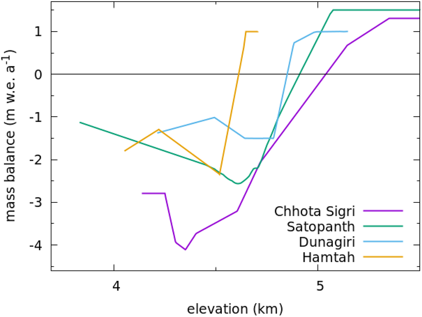
Fig. 3. The mass-balance profiles for the four modeled glaciers.
Dunagiri glacier
For Dunagiri Glacier (Fig. 2b), a long-term retreat rate of 9 ± 0.6 m a−1 has been reported (Kumar and others, Reference Kumar, Mehta, Mishra and Trivedi2016) for the period 1962–2013. Field data on the surface velocities and mass-balance profile are available for the period 1984–90 (Srivastava and Swaroop, Reference Srivastava and Swaroop1992). We use the data of 1986/87 as the corresponding mass balance is similar to the mean mass balance for the whole observation period – a value of −1.0 m w.e. a−1. The mass-balance profile used (Fig. 3) is a piece-wise linear approximation of the data. The surface profile of the glacier along the central flowline is obtained using the 50 m contour map available for the year 1986/87 (Srivastava and Swaroop, Reference Srivastava and Swaroop1992). In this glacier, the added avalanche is spread uniformly over the first kilometer of the glacier during experiment (1).
Hamtah glacier
Hamtah Glacier (Fig. 2c) has previously been studied by two of the authors (AB and RS) to derive an estimate of the avalanche contribution of 1.3 ± 0.1 m w.e. a−1 on that glacier (Banerjee and Shankar, Reference Banerjee and Shankar2014). The method was based on a highly simplified flowline model and depended crucially on a relatively uncertain estimate of the steady-state length of the glacier corresponding to the recent mass balance. We have recomputed the avalanche strength on this glacier using the method described here. We now use a more detailed area-elevation distribution, a piece-wise linear bedrock and the surface profile data from SRTM1 DEM (Farr and others, Reference Farr2007). Also, in the present calculation only an initial transient state is used, without any assumption about a nearby steady state.
The velocity data for the glacier is again from remote-sensing measurements (Scherler and others, Reference Scherler, Bookhagen and Strecker2011b) and the central flowline profile and the glacier hypsometry are extracted from SRTM1 (Farr and others, Reference Farr2007). The long-term front-averaged retreat rate for the glacier is 25.5 m a−1 during 1963–2010 (Pandey and others, Reference Pandey, Venkataraman and Shukla2011) and the recent glaciological net balance is −1.45 m w.e. a−1 during 2000–09 as measured by Geological Survey of India (Shukla and others, Reference Shukla, Mishra and Chitranshi2015). However, during 1989–2010 the front averaged retreat rate has come down to 13 m a−1 (Pandey and others, Reference Pandey, Venkataraman and Shukla2011). The mass-balance profile used in the simulation is a linear approximation of the available data for the mass-balance year 2008/09 (Banerjee and Shankar, Reference Banerjee and Shankar2014), that has similar mass balance as the mean value for the whole period. Avalanche contribution is again uniformly distributed over the grid points within the first kilometer from the top of the glacier.
Chhota Shigri glacier
In Chhota Shigri Glacier, where any significant avalanche contribution is not expected as argued before, a retreat rate of 25 m a−1 for the period of 1972–2006 (Ramanathan, Reference Ramanathan2011), a geodetic mass balance of − 0.17 ± 0.09 m w.e. a−1 during 1988–2010, and a glaciological mass balance of $ - 0.57 \pm 0.40\,{\kern 1pt} {\rm m}\,{\rm w}{\rm. e}{\rm.} \,{\rm a}^{ - 1}$
during 2002–12 (Azam and others, Reference Azam2014) have been reported. The observed mean ELA during the period of 2002–10 is 5075 m (Azam and others, Reference Azam2012). The velocity data for the glacier is obtained from remote-sensing measurements (Scherler and others, Reference Scherler, Bookhagen and Strecker2011b) and the central flowline profile and the glacier hypsometry are from SRTM1 (Farr and others, Reference Farr2007). To make the highest elevation of the selected central flowline consistent with the SRTM1 DEM-derived glacier hypsometry, we shift the elevation and velocity profile by a horizontal distance of 850 m.
$ - 0.57 \pm 0.40\,{\kern 1pt} {\rm m}\,{\rm w}{\rm. e}{\rm.} \,{\rm a}^{ - 1}$
during 2002–12 (Azam and others, Reference Azam2014) have been reported. The observed mean ELA during the period of 2002–10 is 5075 m (Azam and others, Reference Azam2012). The velocity data for the glacier is obtained from remote-sensing measurements (Scherler and others, Reference Scherler, Bookhagen and Strecker2011b) and the central flowline profile and the glacier hypsometry are from SRTM1 (Farr and others, Reference Farr2007). To make the highest elevation of the selected central flowline consistent with the SRTM1 DEM-derived glacier hypsometry, we shift the elevation and velocity profile by a horizontal distance of 850 m.
RESULTS AND DISCUSSIONS
Below, we discuss the results obtained from the above model runs for each of the glaciers modeled. Corresponding observed and modeled surface profile and velocity profiles are shown in Figs 4, 5. The results are also summarised in Table 2.
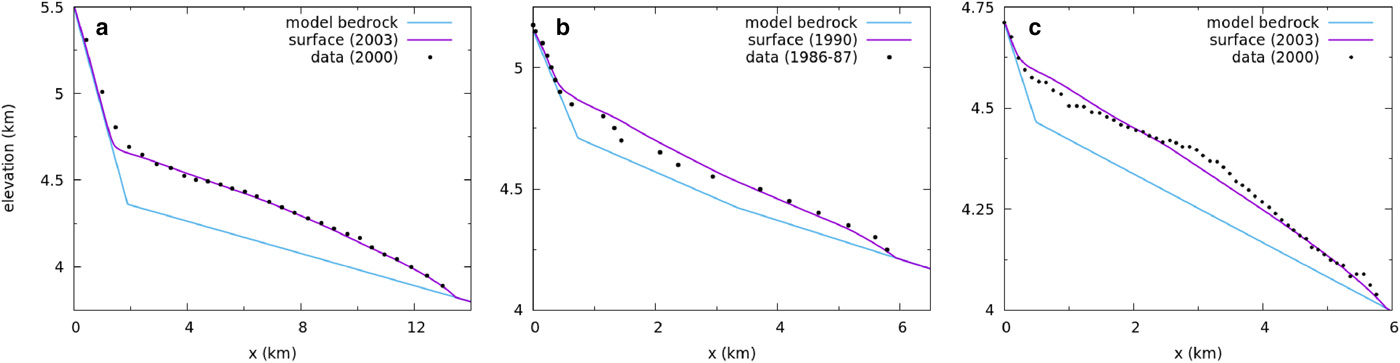
Fig. 4. The comparison of the observed and modeled surface elevation profiles for the recent states of (a) Satopanth, (b) Dunagiri and (c) Hamtah Glaciers. Note different horizontal scale in panel (a).
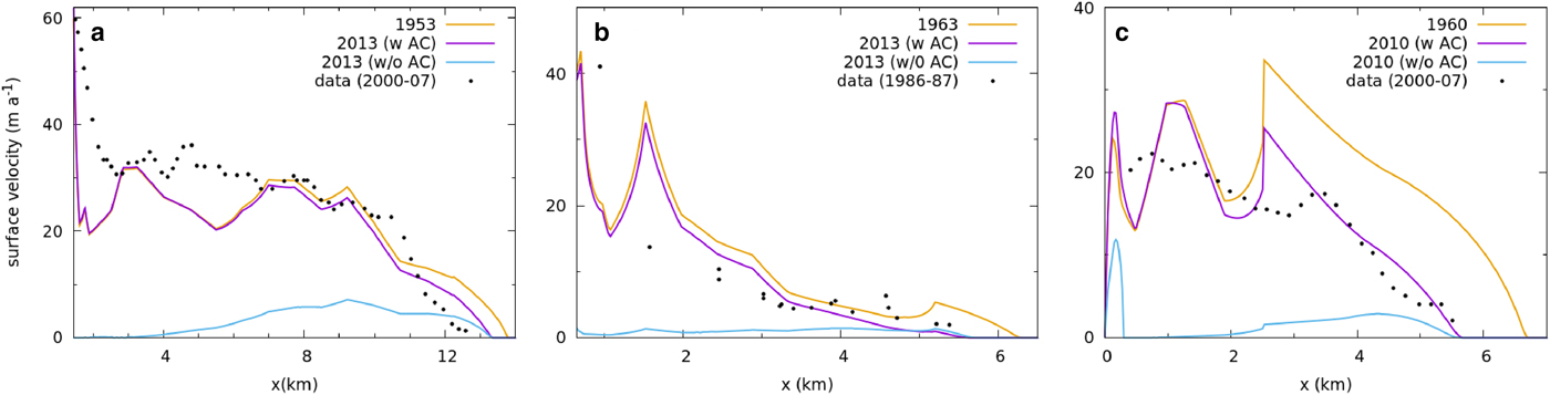
Fig. 5. The modeled velocity profile (solid line) for (a) Satopanth, (b) Dunagiri and (c) Hamtah glacier for the initial and recent states are shown for the runs with and without added avalanche contribution (AC). The dots denote available velocity data.
Table 2. Model parameter and results
Satopanth glacier
The simulated recent state of Satopanth glacier has a mass balance of −2.0 m w.e. a−1 if only the glaciological estimate is considered. However, in experiment (1) a net avalanche contribution of 1.8 m w.e. a−1 is needed to produce a mean retreat rate of 7.5 m a−1 and a net thinning of the lower ablation zone by 0.18 m w.e. a−1 during 1960–2010, which are similar to the corresponding observed values. Without any additional avalanche term (experiment (2)), the glacier thins fast with rates of 2.0 m w.e. a−1 during 1960–2010. Moreover, the ice-flow velocity at the upper ablation zone vanishes quickly, leading to a complete detachment off the lower part (Fig. 5a). Any such detachment or strong slowdown has not been observed in the field. For example, our recent measurements of surface flow velocities during 2014/15 on the upper stakes indicate healthy velocities of more than 50 m a−1. Therefore, the present retreating state of this glacier is not that far away from a steady state and is getting nourished by an avalanche contribution with an estimated magnitude of the order of 1.8 m w.e. a−1. This contribution added to the glaciological mass balance yields a residual of −0.2 m w.e. a−1, which is a revised estimate for recent mass balance of this glacier. A possible geodetic mass-balance measurement can be used to verify this claim. Remarkably, the frontal retreat rate remains the same in both the experiments – this is not unexpected as due to a long response time and low ice flow velocities near the terminus, the retreat rate is chiefly controlled by the local ice-thickness profile in the lowermost part the glacier.
Dunagiri glacier
In Dunagiri glacier, where the recent glaciological mass balance is −1.0 m w.e. a−1, a avalanche contribution of 0.7 m w.e. a−1 is necessary to obtain a realistic retreat rate of 12.5 m a−1 over the past 50 years (Fig. 5b). Without the avalanche term, this glacier displays a thinning rate of −1.0 m w.e. a−1 and flow velocity reduces rapidly all across the ablation zone. The future runs again suggest a complete detachment of the ablation zone from the headwall within 20 years (Fig. 5b). Though velocity data is not available for the current decade to crosscheck, a slowdown by a factor of 5 or more in the upper ablation zone over the past 20 years, and a complete detachment of the ablation zone over the next 20 years seem unlikely. Therefore, it is likely that the mass balance of the glacier over past 50 years is in fact ~−0.3 m w.e. a−1, the residual obtained by adding the avalanche contribution to glaciological mass balance.
Hamtah glacier
In Hamtah glacier, we estimate an avalanche contribution of 1.0 m w.e. a−1, by requiring that the state has right elevation (2000) and velocity profile (~2003), and shows reasonable retreat rates. Our modeled retreat rates for the period 1963–2013 is 22 m a−1 (Fig. 5c), which compares favourably with the observed long-term retreat (Pandey and others, Reference Pandey, Venkataraman and Shukla2011). We do not attempt to fit the recent slowdown of the retreat discussed previously, as we are interested in the long-term mean behaviour of the glacier. This modeled state has a residual mass balance of −0.5 m w.e. a−1 once the avalanche term is included. According to the experiment (2), without such significant avalanche feeding, the initial glacier state form 1963 would have slowed down dramatically, with the ablation area getting completely detached by now (Fig. 5c).
Chhota Shigri glacier
In Chhota Shigri Glacier, where no significant avalanche contribution is expected as discussed before, we have modeled the glacier without any avalanche term and reproduced the observed dynamics of the glacier with just the glaciological mass-balance profile (Fig. 6) (Azam and others, Reference Azam2014). In this case, we start with a longer steady state (ELA ~ 4900 m) and apply a step rise of ELA by 150 m. Then an intermediate state is chosen such that it has the right length, retreat rate, thickness and velocity profile. The modeled glacier has an ELA of 5040 m consistent with the observed mean ELA of 5075 m during the period of 2002–10 (Azam and others, Reference Azam2012). The simulated glacier shows a retreat of 22.6 m a−1 from 1990 to 2010, with a mass balance of −0.6 m w.e. a−1. This modeled retreat rate is comparable with observed retreat rate of 25 m a−1 for the period of 1972–2006 (Ramanathan, Reference Ramanathan2011). On the other hand, the geodetic mass balance of − 0.17 ± 0.09 m w.e. a−1 during 1988–2010 is somewhat smaller than the modeled value. However, the reported glaciological mass balance of − 0.57 ± 0.40 m w.e. a−1 during 2002–12 (Azam and others, Reference Azam2014) and geodetic mass balance of − 0.5 ± 0.3 m w.e. a−1 during 2000–12 (Vijay and Braun, Reference Vijay and Braun2016) match the modeled value. The match of the surface-elevation profile and velocity profile are also reasonable (Fig. 6). The result of this control experiment for a glacier where avalanches are expected to be insignificant, provides strong support for the general validity of our method.
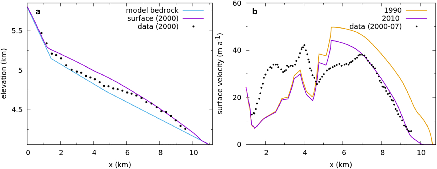
Fig. 6. (a) Comparison of the observed and modeled surface elevation profiles for the recent states Chhota Shigri Glacier. (b) The modeled velocity profile (solid line) for the initial and recent states are shown. The dots denote the observed velocities for the corresponding recent state.
Model sensitivity
For all the three glaciers we repeated the experiments with different values of the tunable parameters like f s, f d, s, and also considered the effect of a 10% uncertainty of the observed retreat rate and a 10% uncertainty of the mass-balance profile. It turns out that in the model glacier the flow is dominated by slip. Therefore, the uncertainty of the values of f d does not affect our result. On the other hand, changing f s by ~10% disturbs the match between observed and modeled velocity and thickness profile. However, the match can be restored by changing s on the lower part of the bedrock by ~2%. These adjustments of f s and s changes the estimated avalanche contribution by ~10%, depending on the glacier and the actual values of the parameter. Allowing an uncertainty of retreat rates of the order of 10%, leads to an uncertainty of the estimated avalanche contribution that is <10%. Other possible sources of uncertainty that are harder to take into account are the effects actual bedrock shape, tributary geometry, the shape of the mass-balance profile used and so on. To check the dependence on the mass-balance profile, we apply constant shifts to the profile by ~10% of the mass balance. This leads to a variation of our avalanche estimate by ~12%. Therefore, we expect an uncertainty of at least ~30% in the estimated avalanche contributions. However, a larger mass-balance uncertainty would lead to a correspondingly higher uncertainty of the avalanche-strength estimate. Thus the long-term avalanche contributions to accumulation on Satopanth, Dunagiri, and Hamtah glacier are estimated to be 1.8 ± 0.5, 0.7 ± 0.2 and 1.0 ± 0.3 m w.e. a−1 respectively.
Consistency with other available data
Mass balance
The glaciological mass balance for the two Central Himalayan glaciers, Satopanth and Dunagiri Glaciers, are −2.0 m w.e. a−1 during 2014/15 and −1.0 m w.e. a−1 during 1984–90, respectively. The other suspected avalanche-fed Western Himalayan glacier modeled here, Hamtah Glacier, has a mass balance of −1.45 m w.e. a−1 during 2000–09 (Shukla and others, Reference Shukla, Mishra and Chitranshi2015). In fact, these are three of the most negative mass-balance values observed in the region (Vincent and others, Reference Vincent2013). These values are considerably more negative than estimated region-wide mean mass balance of −0.5 m w.e. a−1 in the Himalaya (Cogley, Reference Cogley2011). This is consistent with the possibility that significant accumulation contribution due to a putative avalanche activity in these glaciers might have been missed.
Unlike glaciological method, geodetic method captures glacier-wide changes, whether or not avalanche contributions are present. Therefore, if our method of estimating avalanche contribution is correct, then our estimated avalanche contribution for these three glaciers, when added to the glaciological mass balance should lead to residuals that are similar to the corresponding geodetic mass balance. Indeed, the residual mass balance of −0.2, −0.3 and −0.5 m w.e. a−1 on Satopanth, Dunagiri and Hamtah Glacier, respectively, are similar to the existing independent geodetic mass-balance estimates. For example, regional-scale geodetic mass-balance estimates from the Western and Central Himalayan glaciers point to a mass loss of 0.33–0.65 m w.e. a−1 over the past one to four decades (Bolch and others, Reference Bolch, Pieczonka and Benn2011; Kääb and others, Reference Kääb, Berthier, Nuth, Gardelle and Arnaud2012; Gardelle and others, Reference Gardelle, Berthier, Arnaud and Kääb2013; Vincent and others, Reference Vincent2013; Vijay and Braun, Reference Vijay and Braun2016). Also, on Hamtah glacier, the geodetic mass balance during 2000–11 is − 0.45 ± 0.16 m w.e. a−1 (Vincent and others, Reference Vincent2013). This consistency of the residual mass-balance values for the three glaciers computed here, with the known geodetic mass-balance measurements indicates reliability of our method of estimating avalanche contribution. In contrast on Chhota Shigri glacier, where no significant avalanche activity is unlikely, all the three estimates namely, the modeled, geodetic and glaciological mass balances are mutually consistent.
The total avalanche contribution and regional precipitation
A naive expectation regarding the magnitude of the suspected avalanche accumulation is that it should be similar to or less than the total precipitation over the whole avalanche-contributing zone. We compute the ratio of the estimated avalanche accumulation to the product of mean Tropical rainfall measuring mission (TRMM) precipitation and the area of the avalanche-release zone for all the three glaciers. However, the possible uncertainty associated with TRMM precipitation data from the high Himalaya and a potential intensification of precipitation through strong orographic effects due to the high headwalls would mean that theses values are only ball-park estimates. We find that the calculated ratios are ~1.3 ± 0.4, 0.6 ± 0.2 and 1.8 ± 0.5 for Satopanth, Dunagiri and Hamtah Glaciers, respectively. While these values indicate that our estimates are broadly consistent with the potential avalanche accumulation as estimated from local TRMM precipitation rate, they are somewhat larger for Hamtah and Satopanth Glaciers. In spite of the possible uncertainties in the computed ratio, this discrepancy suggests a potential bias in our estimates of the avalanche strength using a simplified flowline model. For example, in Satopanth glacier there are a few tributaries that join the main trunk glacier in the middle ablation zone (Fig. 2a). While modeling the glacier, we have approximated this geometry by that of a simple glacier that shares an identical hypsometry, ignoring the actual tributary configurations. That could be a possible source of the bias for this glacier. However, Hamtah does not have any such complication. We shall investigate these issues further and attempt possible refinements of the flowline model to include the tributaries explicitly in future.
Avalanche control of the glacier dynamics
The results of our simulations for Hamtah, Satopanth and Dunagiri Glaciers indicates that in these glaciers, extensive avalanches from the vast headwalls contribute more than 95% of the total accumulation. Therefore, in the long term such avalanche contributions control both the dynamics and the glacier extent. Despite the large uncertainties in our estimates arising out of the assumptions and simplifications involved in our method and limitations due to a lack detailed data, these results underline the necessity of quantification of the magnitude of the avalanche-derived accumulation on a large class of Himalayan glaciers. This is necessary to explain the present length, thinning and retreat patterns of these glaciers. Further, it is also important to develop a scheme to relate the trends of avalanche accumulation to climate variables at the scale of the whole Himalaya. That problem requires progress both in terms of theoretical tools and direct field observation techniques. In this regard, the existing methods of estimating gravitational redistribution of snow [e.g. Gruber, Reference Gruber2007; Bernhardt and Schulz, (Reference Bernhardt and Schulz2010)], in combination with methods similar to the one presented here could be useful starting points.
CONCLUSIONS
We have discussed the importance of avalanche derived accumulation on a large class of Himalayan glaciers and the diagnostic criteria to identify such glaciers. Using standard glaciological mass-balance techniques, measurement of this avalanche contribution to the mass balance is extremely difficult. Motivated by that, we have described a simplified numerical flowline model-based method that allows a first order estimation of such an avalanche contribution. The method utilises the available long-term data on glacier dynamics and determines a missing mass-balance term necessary to make the recent multi-decadal dynamics consistent with the glaciological mass balance. Our simplified models for three Himalayan glaciers, namely, Satopanth, Dunagiri and Hamtah Glaciers, demonstrate that the above mentioned avalanche-accumulation contribution dominates the accumulation and exerts overwhelming control over the dynamics of a significant number of Himalayan glaciers. This demands further work on more refined theoretical tools and, more importantly, direct field-measurement techniques to quantify the avalanche activity and their long-term trends in the region. Our control experiment with Chhota Shigri Glacier is consistent with no significant avalanche contribution, asserting the robustness of the method in estimating avalanche contribution to mass balance.
ACKNOWLEDGEMENTS
We thank the anonymous reviewer, reviewer D I Benn and scientific editor Charles Fierz for very helpful suggestions that led to a significant improvement of the manuscript in our view. AB acknowledges support from DST-SERB grant no SB.DGH-71.2013 and DST-INSPIRE Faculty award (IFA-12-EAS-04). The field work on Satopanth Glacier was supported by The Institute of Mathematical Sciences.


 Open access