

1 Introduction
Icebergs can disintegrate in a variety of ways; in this paper we explore how swell passing under an ice island causes it to bend and heave, and examine theoretically the wave height required to propagate a crack. This has important implications for the size distribution of icebergs and sea-ice floes.
2 Observations
2.1 Field work
During the course of a field programme to study the marginal sea ice off the east Greenland coast in September 1978, a landing was made on an ice island (Fig. 1) which had drifted into Kong Oscars Fjord. It was located at 72°12’N., 23°20’W., some 40 km from the fjord mouth. A belt of pack ice 65 km wide protected it from the open sea, but allowed the transmission of a detectable swell of long period. The extreme dimensions were 431 m (EF in Figure 1), and 179 m (CD), and from a measurement of freeboard, a thickness between 30 and 35 m was estimated. No crevasses were visible on the surface, but at some locations along the sides the top surface had curled down towards the sea, and a small piece, which had probably become detached by a Reeh-type calving process (Reference ReehReeh 1968) could be seen to one side.

Fig. 1 A vertical photograph of the ice island. A and B were the experimental sites. EF and CD are 431 m and 179 m respectively. The horizontal edge of the photograph is orientated along the fjord. G is a part of the ice island which has calved off by a Reeh-type mechanism.
Two stations were occupied, A and B in Figure 1. At site A, the heave and the surface-strain changes in one direction were recorded, while simultaneous measurements were made of the local wave spectrum with a wave buoy deployed over the edge of the island. The equipment, excepting the wave buoy, was then moved to the centre, site B, and heave and surface-strain changes only recorded. Data were recorded for about 35 min at site A, and for 20 min at site B. The strainmeter was orientated with its axist pointing in the direction of the swell. In this direction the ice island had a length of 406 m. (Full details of the equipment used are given in the longer version of the paper and in Goodman (in press).)
2.2 Data analysis and results
The analogue records recorded on a RACAL FM tape recorder were replayed using the same tape recorder into an A/D converter connected to a PDP-11 computer via an analogue filter with a cut-off at the Nyquist frequency. The time series was digitized at 0.512 s intervals, and the rezeroing jumps, mean, and trends removed. Then a segment which contained either 2 048 or 4 096 data points was used to generate a finite Fourier transform using a FFT package after the final tenths of the time series had been tapered to reduce side-lobe leakage using the cosine data window of Bingham and others (1967). To reduce the error in the spectral estimate, the energies were grouped in the frequency domain by a factor p, which reduces the error in each spectral estimate by a factor ![]() (Reference Bendat and PiersolBendat and Piersol 1971).
(Reference Bendat and PiersolBendat and Piersol 1971).
Figure 2 shows the power spectral density functions for the wave buoy (a), the ice-island heave at site A (b), and the ice-island heave at site B (c), The units are m2 s; the spectral estimates were divided by 16π4 f 4, where f is the frequency. The gain factor (Reference Bendat and PiersolBendat and Piersol 1971) between the wave buoy and ice-island heave at site A and site B were also computed. The results are shown in Figure 3.

Fig. 2 a (left), b (middle), and c (right). Power spectral density functions for the wave buoy at site A (a), the ice-island heave at site A (b) , and the ice-island heave at site B (c).

Fig. 3 a (upper) and b (lower). The gain factor between the wave buoy and ice-island heave at site A (a), and at site B (b). The wave-buoy record from site A was used to compute (b). The dotted lines are the 95% confidence limits
Figure 4 shows the power spectral density functions for the wave buoy (a), the strain record at site A (b), and the strain record at site B (c). In this case the units of the wave-buoy spectrum are as before (m2 s), but the strain spectra have units of s (the spectral estimates have not been divided by 16π4 f 4). It must be noted that the strain shown in Figure 4 overestimates the true strain by approximately 10%. This is because the wire strainmeter, when placed on a heaving body, displays an acceleration response (Moore and Wadhams, in press). In Figure 5 the strain-spectral estimates have been divided by the wave-amplitude estimates, and are shown as a function of period.

Fig. 4 a (left), b (middle), and c (right). Power spectral density functions for the wave buoy at site A (a), the strain record at site A (b), and the strain record at site B (c).

Fig. 5 The strain amplitude divided by the wave amplitude at the two sites plotted as a function of period. The solid and dotted lines are the theoretical predictions.
3 Discussion
3.1 Heave response
The data shown in Figures 2 and 3 indicate that the ice island behaves as a low pass filter. The local wave spectrum is predominantly a monochromatic swell, with a peak of 17 s, but there is also a secondary swell, with a peak at 12 s, and a slight but detectable sea with frequencies up to 0.14’Hz (7 s). In the full version of the paper, an outline of a possible method for deriving the heave response is given.
3.2 Bending response
In a similar way to the heave-response spectra, the strain spectra illustrated in Figure 4 show a low pass characteristic (although it should be noted that the units of the vertical axis are different).
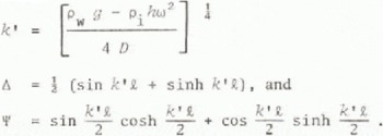
In the full version of the paper, two solutions are given for the bending response of a section in plane strain from a rectangular ice block subject to a pressure field P(x,t) applied along its bottom surface. Both solutions use Froude-Krylov theory whereby the diffraction of waves is ignored. One of us (V.A.S.) is now working on a numerical solution where this restriction is lifted. The first solution finds an analytic expression for the strain amplitude on the surface of the block at its centre when it is subject to a pressure field P(x, t) = ξρW g + AρW gRe[exp(i(kx−ωt))]. ξ is the profile of flexure of the block, and A the amplitude of the water particle motion at the bottom surface. A is related to A’, the wave amplitude on the surface, by the expression A = A’ exp(–khρi/ρW). Then, subject to a set of assumptions, the solution for the strain is:

where
The second solution finds an expression for the surface strain anywhere on the block, subject to a general forcing function P(x, t) as a sum of overlap integrals of P(x, t) and the normal modes of vibration of the block. The solution is not given here, but in Figure 6a the contribution from each normal mode is shown. For ice islands less than 500 m long, or sea-ice floes smaller than 300 m, only the first mode contributes significantly. The normal mode solution also identifies the periods at which there will be a bending resonance between the sea and the ice block. The normal mode periods, Pn are given by the expression

Fig. 6 a (upper), b (middle), and c (lower). Theoretical predictions of the flexural response of the ice island (a), an iceberg (b), and a sea-ice floe (c) as a function of length in the swell direction for a given thickness and wave period. The wave height (peak to trough distance) to make a crack of a given size propagate is shown on the right-hand axis.
where ![]() (Reference Timoshenko, Young and WeaverTimoshenko and others 1974) (n = 1, 3, 5, etc.).
(Reference Timoshenko, Young and WeaverTimoshenko and others 1974) (n = 1, 3, 5, etc.).
3.3 Comparison of bending response theory and observations
If representative values of E (8.72 GN m−2), ν (0.3), l (406 m, the dimension of the ice island in the direction of the swell), h (35 m), and T (17 s, the dominant swell period) are inserted into Equation 1, the bending response (strain amplitude/wave amplitude) as a function of period can be computed. The result is shown in Figure 5 for the centre of the ice island (solid line), and 0.35 l (dotted line). Also shown on the figure are the experimental observations; the agreement is good.
4 The Likelihood of Swell-Induced Fracture
4.1 Critical strain at failure
An ice block has no unique strength; the stress at which failure occurs is a function of the distribution of the cracks that the block contains. This distribution is invariably controlled by the microstructure, which is itself determined by the rate of growth and the strain history. A single crack of length c will propagate when the stress-intensity factor (K Ic) reaches a critical value. The stress-intensity factor is a measure of the stress concentration near a crack, and is related to the local average stress σO and the crack length by the relation
where Ω is a constant which depends on the geometry of the free surfaces and is of order one. A critical discussion of how and when elastic fracture mechanics can be applied to ice is presented by Reference Goodman and TrydeGoodman (1980), who gives a representative value for K Ic for pure ice as 115 kN m−3/2. Then, if c is taken to be equal to the grain size, and, considering the worst case where the period of the forcing function is so short that there is no time for creep to relax the stresses (a purely elastic response), the critical strain εcrit which will cause the crack to propagate is:
which, for c = 1 mm (a typical grain size) , Ω = 1, E = 8.72 GN m−2, and ν = 0.31 is
For sea ice, any crack will bo filled with salt water and K Ic will be reduced. As no satisfactory measurements of K Ic exist for sea ice, suppose K Ic = 50 kN m−3/2, ν = 0.31 and E = 6 GN m−2 (this will depend on brine volume), and suppose c = 10 mm, then
(During the field experiment a direct observation of the strain at failure of a sea-ice floe was made; the value observed was close to 3 × 10⁻⁵.)
4.2 The break-up of ice islands by the action of swell
The bending-response theory, and the critical strain given in the last section can be combined to find a critical wave height at which cracks (in this case 1 mm in length) will propagate. For h = 35 m, and T = 17 s the bending response theory has been used to plot in Figure 6a strain/(wave amplitude) as a function of length (in the swell direction) using E = 8.72 GN m−2, ν = 0.31, ρi = 910 kg m−3, and ρw − 1 025 kg m−3. Then, on the right hand axis the wave height required to propagate a one-millimetre crack is shown.
Cracks of this size are certain to occur on the surface of an ice island. For a given wave height the curve predicts the range of dimensions at which break-up is likely to occur. For instance if ice islands with a wide distribution of sizes pass through a region where the maximum wave height is 10 m, ice islands with any dimension between 490 and 760 m will not survive the passage. If the wave height is 20 m, the critical range where failure might occur is extended to 380–840, 1 020–1 140, and 1 350–1 760 m. Finally, if there is a likelihood of 30 m waves, only ice islands with dimensions within the range 0 to 340 m and 1 840 to 2 160 m will survive. Then, if a calving glacier generates a wide distribution of ice-island sizes, after a short exposure to sea swell the distribution would exhibit some of the features in Figure 6a. Dimensions close to 915 m and 1 246 m are particularly favourable. But the majority of ice islands of this thickness would continue to calve until none of their dimensions was greater than about 400 m.
The ultimate failure will be a type of fatigue process. During part of each wave cycle, cracks will grow, reducing εcrit. For each successive cycle the cracks will grow for a larger proportion of the cycle until eventually one crack will propagate unstably. The increasing hydrostatic pressure with depth will tend to arrest downward-growing cracks, but water-filled cracks at the bottom do not suffer this disadvantage and have a lower K Ic. Consequently the failure will probably originate at the bottom.
The solution for the bending response may also be used to examine the effect of change of thickness on the survival of the ice island. In Figure 7 the strain/(wave amplitude) is plotted as a function of thickness for various lengths in the swell direction using the same values of E, ν, ρw, ρi, and T as Figure 5a. The curves show that, as the ice island thins by melting, there is a rapid rise in the surface strain for a fixed wave amplitude (the beam cross-section is smaller for the same load, and so the strain is larger). Again on the right-hand axis the wave height required to propagate a one-millimetre crack is shown.

Fig. 7 The strain amplitude/(wave amplitude) plotted as a function of thickness for a given length and period.
4.3 Extension of the theory to icebergs and ice floes
The theory developed in the longer paper can be very appropriately applied to sea-ice floes. Figure 6c shows the strain/(wave amplitude) as a function of length in the swell direction for a three-metre thickness, and wave period of 12 and 17 s (calculated using E/(1−ν2) = 6 MN m−2, ρw = 910 kg m−3, ρi = 1 025 kg m−3). On the right-hand axis the wave height required to propagate a ten-millimetre crack is shown. Only small wave heights are required to fracture a floe; large floes will rapidly break up into a size range given by OB (0 to 220 m) for wave heights greater than 0.15 m of 12 s period. This is in good accord with observations of floe size distributions.
The theory can also be applied to tabular icebergs, although a Froude-Krylov theory introduces large errors in this case. Further, only the longest swells penetrate deeply enough to cause an oscillating pressure field on the iceberg bottom. Figure 6b is the result of solving the theory for an iceberg 100 m thick, deformed by a 24 s swell, which is typical of the longest swells found in the Southern Ocean. To propagate a one-millimetre crack requires a wave height of about 20 m, which is a rare event even in the Southern Ocean for a 24 s swell (a 17 s swell requires a fetch of 2 000 km, and a wind speed of 30 m s−1 to reach 20 m). Therefore, the question can be reversed, and instead the crack size that a three-metre wave will propagate calculated. This is given by the expression:
If 2A’ is 3 m, and l for the iceberg is 1 km, c crit has the value of 66 mm. Cracks of this size would not be uncommon in a large iceberg. Thus icebergs would continue to calve until their maximum dimension lies somewhere in the range of the early part of the curve, 0C (0 to 1 km). This is in agreement with the observations by Landsat imagery in the open water of the Southern Ocean that most icebergs have dimensions no greater than 1.3 km (Reference Hult, Ostrander, Freden, Mercanti and BeckerHult and Ostrander 1974, Reference Weeks and MellorWeeks and Mellor 1978).
5 Conclusions
We conclude that wave-induced flexural failure could well be the cause of the scarcity of icebergs with diameters greater than about 2 km in the open Southern Ocean. Very large icebergs are likely to suffer multiple fractures of this nature in a stormy sea or heavy swell, until all the fragments are less than a critical diameter. A long narrow iceberg several km long and 1 to 4 km wide is likely to fracture in a lesser sea if it is allowed to come beam on to the waves so that the length presented to the sea falls into one of the unstable regions A and B of Figure 6b.
The towing of an iceberg or ice island in open water is likely to be hazardous because of the likelihood of wave-induced fracture, and it is recommended that continuous monitoring of surface-strain changes should be made.
Acknowledgements
The authors gratefully acknowledge the assistance of S.C. Moore and S. Overgaard in the field work, and of the helicopter pilot, B. Andersson of Greenlandair, We also wish to acknowledge support from the Office of Naval Research under Contract N00014-78-G-0003, and the Natural Environment Research Council. We are grateful to R.J. Horne for developing the computer package used for the data analysis, and for the assistance of R. Weintraub and A.M. Cowan. We thank C.S. Neal for his assistance during the construction of the amplifier system. D.J. Goodman is grateful for research fellowships, from the Science Research Council and Girton College, for research grants from the Science Research Council and the Royal Society, and to Professor A. Higashi and the Japan Society for the Promotion of Science for allowing him to visit Hokkaido University where part of this work was completed.


